Explicit Structure-Preserving Geometric Particle-in-Cell Algorithm in Curvilinear Orthogonal Coordinate Systems and Its Applications to Whole-Device 6D Kinetic Simulations of Tokamak Physics

Abstract

Explicit structure-preserving geometric Particle-in-Cell (PIC) algorithm in curvilinear orthogonal coordinate systems is developed. The work reported represents a further development of the structure-preserving geometric PIC algorithm (Squire et al., 2012a, b; Xiao et al., 2013, 2015a, 2015b; He et al., 2015a; Qin et al., 2016; He et al., 2016a; Kraus et al., 2017; Xiao et al., 2017, 2018; Xiao and Qin, 2019a), achieving the goal of practical applications in magnetic fusion research. The algorithm is constructed by discretizing the field theory for the system of charged particles and electromagnetic field using Whitney forms, discrete exterior calculus, and explicit non-canonical symplectic integration. In addition to the truncated infinitely dimensional symplectic structure, the algorithm preserves exactly many important physical symmetries and conservation laws, such as local energy conservation, gauge symmetry and the corresponding local charge conservation. As a result, the algorithm possesses the long-term accuracy and fidelity required for first-principles-based simulations of the multiscale tokamak physics. The algorithm has been implemented in the SymPIC code, which is designed for high-efficiency massively-parallel PIC simulations in modern clusters. The code has been applied to carry out whole-device 6D kinetic simulation studies of tokamak physics. A self-consistent kinetic steady state for fusion plasma in the tokamak geometry is numerically found with a predominately diagonal and anisotropic pressure tensor. The state also admits a steady-state sub-sonic ion flow in the range of 10 km/s, agreeing with experimental observations (Ince-Cushman et al., 2009; Rice et al., 2009) and analytical calculations (Guan et al., 2013a, b). Kinetic ballooning instability in the self-consistent kinetic steady state is simulated. It shows that high-n ballooning modes have larger growth rates than low-n global modes, and in the nonlinear phase the modes saturate approximately in 5 ion transit times at the 2% level by the $E\times B$ flow generated by the instability. These results are consistent with early (Qin, 1998; Qin et al., 1999a) and recent (Dong et al., 2019) electromagnetic gyrokinetic simulations.

I Introduction

Six Dimensional (6D) Particle-In-Cell (PIC) simulation is a powerful tool for studying complex collective dynamics in plasmas (Dawson, 1983; Hockney and Eastwood, 1988; Birdsall and Langdon, 1991). However, as a first-principles-based numerical method, 6D PIC simulation has not been employed to study the dynamical behavior experimentally observed in magnetic fusion plasmas, mainly due to the multiscale nature of the physics involved. The technical difficulties are two-fold. First, the span of space-time scales of magnetic fusion plasmas is enormous, and numerically resolving these space-time scales demands computation hardware that did not exist until very recently. Secondly, even if unlimited computing resource exists, the standard 6D PIC algorithms do not posses the long-term accuracy and fidelity required for first-principles-based simulations of magnetic fusion plasmas. For example, the most commonly used 6D PIC scheme is the Boris-Yee scheme, which solves the electromagnetic fields using the Yee-FDTD (Yee et al., 1966) method and advances particles’ position and velocity by the Boris algorithm (Boris, 1970). Even though both Yee-FDTD method (Stern et al., 2015) and the Boris algorithm (Qin et al., 2013; He et al., 2015b; Zhang et al., 2015; Ellison et al., 2015a; He et al., 2016b; Tu et al., 2016) themselves do have good conservative properties, their combination in PIC methods does not (Hockney and Eastwood, 1988; Birdsall and Langdon, 1991; Ueda et al., 1994). Numerical errors thus accumulate coherently during simulations and long-term simulation results are not trustworthy.

Recent advances in super-computers (Fu et al., 2016) have made 6D PIC simulation of magnetic fusion plasmas possible in terms of hardware. On the other hand, much needed now is modern 6D PIC algorithms that can harness the rapidly increasing power of computation hardware. A family of such new 6D PIC algorithms (Squire et al., 2012a, b; Xiao et al., 2013, 2015a, 2015b; He et al., 2015a; Qin et al., 2016; He et al., 2016a; Kraus et al., 2017; Xiao et al., 2017, 2018; Xiao and Qin, 2019a) has been developed recently. Relative to the conventional PIC methods, two unique properties characterize these new PIC algorithms: the space-time discretization is designed using modern geometric methods, such as discrete manifold and symplectic integration, and the algorithms preserve exactly many important physical symmetries and conservation laws in a discrete sense. For this reason, these algorithms are called structure-preserving geometric PIC algorithms. The long-term accuracy and fidelity of these algorithms have been studied and documented by different research groups (Xiao et al., 2015a; Kraus et al., 2017; Morrison, 2017; Holderied et al., 2020; Xiao and Qin, 2019b; Li et al., 2019, 2020; Hirvijoki et al., 2020; Perse et al., 2020; Zheng et al., 2020a; Wang et al., 2020; Kormann and Sonnendrücker, 2021).

Discrete symplectic structure and symplectic integration are two of the main features of the structure-preserving geometric PIC algorithms. Up to now, the only explicit symplectic integrator for the non-canonical symplectic structure of the discrete or continuous Vlasov-Maxwell system is the splitting method developed in Ref. (He et al., 2015a), which splits the dynamics symplectically into one-way decoupled Cartesian components. The requirement of the Cartesian coordinate system creates a hurdle for applications in magnetic fusion plasmas, for which cylindrical or toroidal coordinate systems are more convenient. Most simulation codes, such as GTC (Lin et al., 1998; Zebin et al., 2013), XGC (Ku et al., 2006; Chang et al., 2009) and GEM (Chen and Parker, 2003, 2007; Wang et al., 2012) adopted curvilinear coordinate systems. In the present study, we extend the structure-preserving geometric PIC algorithm to arbitrary curvilinear orthogonal coordinate systems, in particular, to the cylindrical coordinate system for applications in tokamak physics. We show that when a sufficient condition (75) is satisfied, which is the case for the cylindrical mesh, the structure-preserving PIC algorithm can be made explicitly solvable and high-order. For easy implementation and presentation, we first present the algorithm as a discrete field theory (Lee, 1983, 1987; Veselov, 1988; Marsden and West, 2001; Han-Ying et al., 2002; Qin, 2020) specified by a Lagrangian discretized in both space and time. It is then reformulated using a generalized version of the discrete Poisson bracket developed in Ref. (Xiao et al., 2015a) and an associated explicit symplectic splitting algorithm, which generalizes the original algorithm designed in Ref. (He et al., 2015a) in the Cartesian coordinate system. In particular, the technique utilizing the one-way decoupling of dynamic components is generalized to arbitrary curvilinear orthogonal coordinate systems satisfying condition (75).

The algorithm has been implemented in the the SymPIC code and applied to carry out whole-device 6D kinetic PIC simulations of plasma physics in a small tokamak with similar machine parameters as the Alcator C-Mod (Hutchinson et al., 1994; Greenwald et al., 1997). We numerically study two topics: self-consistent kinetic steady state in the tokamak geometry and kinetic ballooning instability in the edge. Simulation shows that when plasma reaches a self-consistent kinetic steady state, the pressure tensor is diagonal, anisotropic in 3D, but isotropic in the poloidal plane. A sub-sonic ion flow in the range of $10$km/s exists, which agrees with experimental observations (Ince-Cushman et al., 2009; Rice et al., 2009) and theoretical calculations (Guan et al., 2013a, b). In the self-consistent kinetic steady state, it is found that large-$n$ kinetic ballooning modes grow faster than low-$n$ global modes, and the instability saturates nonlinearly at the 2% level by the $E\times B$ flow generated by the instability. These results qualitatively agree with previous simulations by electromagnetic gyrokinetic codes (Qin, 1998; Qin et al., 1999a; Dong et al., 2019).

Because the algorithm is based on first-principles of physics and constructed in general geometries, the whole-device 6D kinetic simulation capability developed is applicable to other fusion devices and concepts as well, including stellarators, field reserve configurations and inertial confinement. It is also worthwhile to mention that the structure-preserving geometric discretization technique developed for the 6D electromagnetic PIC simulations can be applied to other systems as well, including ideal two-fluid systems (Xiao et al., 2016) and magnetohydrodynamics (Zhou et al., 2014, 2016; Zhou, 2017; Zhou et al., 2017a; Burby and Tronci, 2017). Structure-preserving geometric algorithms have also been developed for the Schrödinger-Maxwell (Chen et al., 2017) system, the Klein-Gordon-Maxwell system (Shi et al., 2016, 2018; Shi, 2018; Shi et al., 2020), and the Dirac-Maxwell system (Chen and Xiao, 2019), which have important applications in high energy density physics. Another noteworthy development is the metriplectic particle-in-cell integrators for the Landau collision operator (Hirvijoki et al., 2018). Recently, a field theory and a corresponding 6D structure-preserving geometric PIC algorithm were established for low-frequency electrostatic perturbations in magnetized plasmas with adiabatic electrons (Xiao and Qin, 2019a). The long-term accuracy and fidelity of the algorithm enabled the simulation study of electrostatic drift wave turbulence and transport using a 6D PIC method with adiabatic electrons.

The paper is organized as follows. In Sec. II we develop the explicit structure-preserving geometric PIC scheme in arbitrary orthogonal coordinate systems, and the algorithm in a cylindrical mesh is implemented in the SymPIC code. In Sec. III, the code is applied to carry out whole-device 6D kinetic PIC simulations of tokamak physics.

II Explicit structure-preserving geometric PIC algorithm in curvilinear orthogonal coordinate systems

II.1 The basic principles of structure-preserving geometric PIC algorithm

The procedure of designing a structure-preserving geometric PIC algorithm starts from a field theory, or variational principle, for the system of charged particles and electromagnetic field. Instead of discretizing the corresponding Vlasov-Maxwell equations, the variational principle is discretized.

For spatial discretization of the electromagnetic field, discrete exterior calculus (Hirani, 2003; Desbrun et al., 2005) is adopted. As indicated by its name, a PIC algorithm contains two components not found in other simulation methods: charge and current deposition from particles to grid points, and field interpolation from grid points to particles. Note that these two components are independent from the field solver, e.g., the Yee-FDTD method, and the particle pusher, e.g., the Boris algorithm. In conventional PIC algorithms (Dawson, 1983; Hockney and Eastwood, 1988; Birdsall and Langdon, 1991), the function of charge and current deposition and the function of field interpolation are implemented using intuitive techniques without fundamental guiding principles other than the consistency requirement. It was found (Squire et al., 2012a, b; Xiao et al., 2018) that a systematic method to realize these two functions is to apply the Whitney interpolation (differential) forms (Whitney, 1957) and their high-order generalizations (Xiao et al., 2015a) on the discrete Lagrangian.

The application of Whitney forms is a key technology for achieving the goal of preserving geometric structures and conservation laws. It stipulates from first principles how charge and current deposition and field interpolation should be performed (Squire et al., 2012a, b; Xiao et al., 2013, 2015a, 2015b; He et al., 2015a; Qin et al., 2016; He et al., 2016a; Kraus et al., 2017; Xiao et al., 2017, 2018; Xiao and Qin, 2019a). It also enabled the derivation of the discrete non-canonical symplectic structure and Poisson bracket for the charged particle-electromagnetic field system (Xiao et al., 2015a). At the continuous limit when the size of the space-time grid approaches zero, the discrete non-canonical Poisson bracket reduces to the Morrison-Marsden-Weinstein (MMW) bracket for the Vlasov-Maxwell equations (Morrison, 1980; Marsden and Weinstein, 1982; Weinstein and Morrison, 1981; Burby, 2017; Morrison, 2017) (The MMW bracket was also independently discovered by Iwinski and Turski (Iwinski and Turski, 1976)). To derive the discrete Poisson bracket, Whitney forms and their high-order generalizations are adopted for the purpose of geometric spatial discretization of the field Lagrangian density as an 1-form in the phase space of the charged particle-electromagnetic field system, whose exterior derivative automatically generates a discrete non-canonical symplectic structure and consequently a Poisson bracket. As a different approach, He et al. (He et al., 2016a) and Kraus et al. (Kraus et al., 2017) used the method of finite element exterior calculus to discretize the MMW bracket directly, and verified explicitly that the discretized bracket satisfies the Jacobi identity through lengthy calculations, in order for the discretized bracket to be a legitimate Poisson bracket. If one chooses to discretize the MMW bracket directly (Perse et al., 2020; Hirvijoki et al., 2020), such verification is necessary because there are other discretizations of the MMW bracket which satisfy the numerical consistency requirement but not the Jacobi identity. On the other hand, the discrete Poisson bracket in Ref. (Xiao et al., 2015a) was not a discretization of the MMW bracket. It was derived from the spatially discretized 1-form using Whitney forms and is naturally endowed with a symplectic structure and Poisson bracket, and reduces to the MMW bracket in the continuous limit. The advantage of this discrete Poisson bracket in this respect demonstrates the power of Whitney forms in the design of structure-preserving geometric PIC algorithms.

To numerically integrate a Hamiltonian or Poisson system for the purpose of studying multiscale physics, symplectic integrators are necessities. Without an effective symplectic integrator, a symplectic or Poisson structure is not beneficial in terms of providing a better algorithm with long-term accuracy and fidelity. However, essentially all known symplectic integrators are designed for canonical Hamiltonian systems (Devogelaere, 1956; Lee, 1983; Ruth, 1983; Feng, 1985, 1986; Lee, 1987; Sanz-Serna, 1988; Veselov, 1988; Yoshida, 1990; Forest and Ruth, 1990; Channell and Scovel, 1990; Candy and Rozmus, 1991; Tang, 1993; Sanz-Serna and Calvo, 1994; Shang, 1994; Kang and Zai-jiu, 1995; Shang, 1999; Marsden and West, 2001; Han-Ying et al., 2002; Hairer et al., 2002; Hong and Qin, 2002; jiu Shang, 2006; Feng and Qin, 2010; Zhang et al., 2016; Tao, 2016), except for recent investigations on non-canonical symplectic integrators (Qin and Guan, 2008; Qin et al., 2009; Squire et al., 2012c; Zhang et al., 2014; Ellison et al., 2015b; Burby and Ellison, 2017; Kraus, 2017; Ellison et al., 2018; Ellison, 2016; He et al., 2017; Zhou et al., 2017b; Xiao and Qin, 2019c; Shi et al., 2019; Xiao and Qin, 2020) for charged particle dynamics in a given electromagnetic field. Generic symplectic integrators for non-canonical symplectic systems are not known to exist. Fortunately, a high-order explicit symplectic integrator for the MMW bracket was discovered (He et al., 2015a) using a splitting technique in the Cartesian coordinate system. The validity of this explicit non-canonical symplectic splitting method is built upon the serendipitous one-way decoupling of the dynamic components of the particle-field system in the Cartesian coordinate system. It’s immediately realized (Xiao et al., 2015a) that this explicit non-canonical symplectic splitting applies to the discrete non-canonical Poisson bracket without modification for the charged particle-electromagnetic field system. This method was also adopted in Refs. (He et al., 2016a) and (Kraus et al., 2017) to integrate the discretized MMW bracket using finite element exterior calculus. See also Refs. (Crouseilles et al., 2015) and (Qin et al., 2015) for early effort for developing symplectic splitting method for the Vlasov-Maxwell system. It was recently proven (Xiao et al., 2018) that the discrete non-canonical Poisson bracket (Xiao et al., 2015a) and the explicit non-canonical symplectic splitting algorithm (He et al., 2015a) can be equivalently formulated as a discrete field theory (Qin, 2020) using a Lagrangian discretized in both space and time.

The geometric discretization of the field theory for the system of charged particles and electromagnetic field using Whitney forms (Whitney, 1957; Squire et al., 2012b; Xiao et al., 2015a), discrete exterior calculus (Hirani, 2003; Desbrun et al., 2005), and explicit non-canonical symplectic integration (He et al., 2015a; Xiao et al., 2015a) results in a PIC algorithm preserving many important physical symmetries and conservation laws. In addition to the truncated infinitely dimensional symplectic structure, the algorithms preserves exactly the local conservation laws for charge (Squire et al., 2012a, b; Xiao et al., 2018) and energy (Xiao et al., 2017). It was shown that the discrete local charge conservation law is a natural consequence of the discrete gauge symmetry admitted by the system (Squire et al., 2012a, b; Xiao et al., 2018; Glasser and Qin, 2020). The correspondence between discrete space-time translation symmetry (Glasser and Qin, 2019a, b) and discrete local energy-momentum conservation law has also been established for the Maxwell system (Xiao et al., 2019).

As mentioned in Sec. I, the goal of this section is to extend the explicit structure-preserving geometric particle-in-cell algorithm, especially the discrete non-canonical Poisson bracket (Xiao et al., 2015a) and the explicit non-canonical symplectic splitting algorithm (He et al., 2015a), from the Cartesian coordinate systems to curvilinear orthogonal coordinate systems that are suitable for the tokamak geometry.

II.2 Field theory of the particle-field system in curvilinear orthogonal coordinate systems

We start from the action integral of the system of charged particles and electromagnetic field. In a curvilinear orthogonal coordinate system $\left(x_{1},x_{2},x_{3}\right)$ with line element

$$\mathrm{d}s^{2}=h_{1}\left(x_{1},x_{2},x_{3}\right)^{2}\mathrm{d}x_{1}^{2}+h_{2}\left(x_{1},x_{2},x_{3}\right)^{2}\mathrm{d}x_{2}^{2}+h_{3}\left(x_{1},x_{2},x_{3}\right)^{2}\mathrm{d}x_{3}^{2}\ ,$$ (1)

the action integral of the system is

$$\mathcal{A}[\mathbf{x}_{sp},\dot{\mathbf{x}}_{sp},\mathbf{A},\phi] = \int\mathrm{d}t\sum_{s,p}\left(L_{sp}\left(m_{s},\mathbf{v}_{sp}\right)+q_{s}\left(\mathbf{v}_{sp}\cdot\mathbf{A}\left(\mathbf{x}_{sp},t\right)-\phi\left(\mathbf{x}_{sp},t\right)\right)\right)$$ (2)

$$+\int\mathrm{d}V\mathrm{d}t\frac{1}{2}\left(\left(-\dot{\mathbf{A}}\left(\mathbf{x},t\right)-\nabla\phi\left(\mathbf{x},t\right)\right)^{2}-\left(\nabla\times\mathbf{A}\left(\mathbf{x},t\right)\right)^{2}\right)\leavevmode\nobreak\ ,$$

where $\mathbf{x}=[x_{1},x_{2},x_{3}]$ and $\mathrm{d}V=|h_{1}\left(\mathbf{x}\right)h_{2}\left(\mathbf{x}\right)h_{3}\left(\mathbf{x}\right)|\mathrm{d}x_{1}\mathrm{d}x_{2}\mathrm{d}x_{3}$. In this coordinate system, the position and velocity of the $p$-th particle of species $s$ are $\mathbf{x}_{sp}=[{x_{sp_{1}}},{x_{sp_{2}}},{x_{sp_{3}}}]$ and $\mathbf{v}_{sp}=[{\dot{x}_{sp_{1}}}h_{1}\left(\mathbf{x}_{sp}\right),{\dot{x}_{sp_{2}}}h_{2}\left(\mathbf{x}_{sp}\right),{\dot{x}_{sp_{3}}}h_{3}\left(\mathbf{x}_{sp}\right)]$. $L_{sp}$ is the free Lagrangian for the $p$-th particle of species $s$. For the non-relativistic case $L_{sp}=m_{s}|\mathbf{v}_{sp}|^{2}/2$, and for the relativistic case $L_{sp}=-m_{s}\sqrt{1-|\mathbf{v}_{sp}|^{2}}$. Here, we set both permittivity $\epsilon_{0}$ and permeability $\mu_{0}$ in the vacuum to 1 to simplify the notation. The evolution of this system is governed by the variational principle,

$$\frac{\delta\mathcal{A}}{\delta\mathbf{A}} = 0\leavevmode\nobreak\ ,$$ (3)

$$\frac{\delta\mathcal{A}}{\delta\phi} = 0\leavevmode\nobreak\ ,$$ (4)

$$\frac{\delta\mathcal{A}}{\delta\mathbf{x}_{sp}} = 0\leavevmode\nobreak\ .$$ (5)

It can be verified that Eq. (3) and Eq. (4) are the Maxwell equations, and Eq. (5) is Newton’s equation for the $p$-th particle of species $s$.

II.3 Construction of the algorithm as a discrete field theory

According to the general principle of structure-preserving geometric algorithm, the first step is to discretize the field theory (Squire et al., 2012a, b; Xiao et al., 2015a, 2018; Xiao and Qin, 2019a). For the electromagnetic field, we use the technique of Whitney forms and discrete manifold (Whitney, 1957; Hirani, 2003). For example, in a tetrahedron mesh the magnetic field $\mathbf{B}$ as a 2-form field can be discretized on a 2-simplex $\sigma_{2}$ (a side of a 3D tetrahedron mesh) as $\int_{\sigma_{2}}\mathbf{B}\cdot\mathrm{d}\mathbf{S}$, where $\mathbf{S}$ is the unit normal vector of $\sigma_{2}$. Note that $\sigma_{2}$ is a common side of two tetrahedron cells. In a mesh constructed using a curvilinear orthogonal coordinate system, which will be referred to as a Curvilinear Orthogonal Mesh (COM), such discretization can be also performed. Let

$$\phi_{i,j,k,l} = \phi\left(x_{J,l}^{4}\right)\leavevmode\nobreak\ ,$$ (6)

$$\mathbf{A}_{i,j,k,l} = \left[\begin{array}[]{c}A_{x_{1}}\left(x_{J,l}^{4}\right)h_{1}\left(x_{J,l}^{4}\right),\\ A_{x_{2}}\left(x_{J,l}^{4}\right)h_{2}\left(x_{J,l}^{4}\right),\\ A_{x_{3}}\left(x_{J,l}^{4}\right)h_{3}\left(x_{J,l}^{4}\right)\end{array}\right]^{T}\leavevmode\nobreak\ ,$$ (10)

$$\mathbf{B}_{i,j,k,l} = \left[\begin{array}[]{c}B_{x_{1}}\left(x_{J,l}^{4}\right)h_{2}\left(x_{J,l}^{4}\right)h_{3}\left(x_{J,l}^{4}\right),\\ B_{x_{2}}\left(x_{J,l}^{4}\right)h_{3}\left(x_{J,l}^{4}\right)h_{1}\left(x_{J,l}^{4}\right),\\ B_{x_{3}}\left(x_{J,l}^{4}\right)h_{1}\left(x_{J,l}^{4}\right)h_{2}\left(x_{J,l}^{4}\right)\end{array}\right]^{T}\leavevmode\nobreak\ ,$$ (14)

$$\rho_{i,j,k,l} = \rho\left(x_{J,l}^{4}\right)h_{1}\left(x_{J,l}^{4}\right)h_{2}\left(x_{J,l}^{4}\right)h_{3}\left(x_{J,l}^{4}\right)\leavevmode\nobreak\ ,$$ (15)

where $\left(x_{J,l}^{4}\right)$ denotes $\left(i\Delta x_{1},j\Delta x_{2},k\Delta x_{3},l\Delta t\right)$, $\phi_{i,j,k,l},\mathbf{A}_{i,j,k,l},\mathbf{B}_{i,j,k,l}$ and $\rho_{i,j,k,l}$ are discrete 0-, 1-, 2- and 3-forms, respectively. In this discretization, the discrete gradient, curl and divergence operators can simply be finite difference operators. In the present study, the following difference operators are adopted,

$$\left({\nabla_{\mathrm{d}}}\phi\right)_{i,j,k} = [\phi_{i+1,j,k}-\phi_{i,j,k},\phi_{i,j+1,k}-\phi_{i,j,k},\phi_{i,j,k+1}-\phi_{i,j,k}]\leavevmode\nobreak\ ,$$ (16)

$$\left({\mathrm{curl_{d}}}\mathbf{A}\right)_{i,j,k} = \left[\begin{array}[]{c}\left({A_{x_{3}}}_{i,j+1,k}-{A_{x_{3}}}_{i,j,k}\right)-\left({A_{x_{2}}}_{i,j,k+1}-{A_{x_{2}}}_{i,j,k}\right)\\ \left({A_{x_{1}}}_{i,j,k+1}-{A_{x_{1}}}_{i,j,k}\right)-\left({A_{x_{3}}}_{i+1,j,k}-{A_{x_{3}}}_{i,j,k}\right)\\ \left({A_{x_{2}}}_{i+1,j,k}-{A_{x_{2}}}_{i,j,k}\right)-\left({A_{x_{1}}}_{i,j+1,k}-{A_{x_{1}}}_{i,j,k}\right)\end{array}\right]^{T}\leavevmode\nobreak\ ,$$ (20)

$$\left({{\mathrm{div_{d}}}}\mathbf{B}\right)_{i,j,k} = \left({B_{x_{1}}}_{i+1,j,k}-{B_{x_{1}}}_{i,j,k}\right)+\left({B_{x_{2}}}_{i,j+1,k}-{B_{x_{2}}}_{i,j,k}\right)+$$ (21)

$$\left({B_{z}}_{i,j,k+1}-{B_{z}}_{i,j,k}\right)\leavevmode\nobreak\ .$$

To discretize the particle-field interaction while preserving geometric structures and symmetries, Whitney interpolating forms (Whitney, 1957) and their high-order generalizations (Xiao et al., 2015a) are used. Akin to previous results on Whitney interpolating forms in a cubic mesh (Xiao et al., 2015a), interpolating forms $W_{O\sigma_{0}J}\left(\mathbf{x}\right),W_{O\sigma_{1}J}\left(\mathbf{x}\right),W_{O\sigma_{2}J}\left(\mathbf{x}\right)$ and $W_{O\sigma_{3}J}\left(\mathbf{x}\right)$ for 0-, 1-, 2- and 3-forms can be constructed on a COM as follows,

$$W_{O\sigma_{0}J}\left(\mathbf{x}\right) = W_{\sigma_{0}J}\left(\mathbf{x}\right)\leavevmode\nobreak\ ,$$ (22)

$$W_{O\sigma_{1}J}\left(\mathbf{x}\right) = W_{\sigma_{1}J}\left(\mathbf{x}\right)/[h_{1}\left(\mathbf{x}\right),h_{2}\left(\mathbf{x}\right),h_{3}\left(\mathbf{x}\right)]\leavevmode\nobreak\ ,$$ (23)

$$W_{O\sigma_{2}J}\left(\mathbf{x}\right) = W_{\sigma_{2}J}\left(\mathbf{x}\right)/[h_{2}\left(\mathbf{x}\right)h_{3}\left(\mathbf{x}\right),h_{3}\left(\mathbf{x}\right)h_{1}\left(\mathbf{x}\right),h_{1}\left(\mathbf{x}\right)h_{2}\left(\mathbf{x}\right)]\leavevmode\nobreak\ ,$$ (24)

$$W_{O\sigma_{3}J}\left(\mathbf{x}\right) = W_{\sigma_{3}J}\left(\mathbf{x}\right)/h_{1}\left(\mathbf{x}\right)h_{2}\left(\mathbf{x}\right)h_{3}\left(\mathbf{x}\right)\leavevmode\nobreak\ ,$$ (25)

where $W_{\sigma iJ}\left(\mathbf{x}\right),0\leq i\leq 3$ are the interpolating forms in a cubic mesh defined in Ref. (Xiao et al., 2015a) and the quotient (product) of vectors means component-wise quotient (product), i.e.,

$$[A_{x_{1}},A_{x_{2}},A_{x_{3}}]/[B_{x_{1}},B_{x_{2}},B_{x_{3}}] = [\frac{A_{x_{1}}}{B_{x_{1}}},\frac{A_{x_{2}}}{B_{x_{2}}},\frac{A_{x_{3}}}{B_{x_{3}}}]\leavevmode\nobreak\ .$$ (26)

With these operators and interpolating forms, we discretize the action integral as

$$\mathcal{A}_{d} = \sum_{s,p,l}\left(L_{sp}\left(m_{s},\mathbf{v}_{sp,l}\right)+q_{s}\left(\overline{\mathbf{v}_{sp}\cdot\mathbf{A}}\left(\mathbf{x}_{sp,l},\mathbf{x}_{sp,l+1},l\right)-\phi\left(\mathbf{x}_{sp,l+1},l+1\right)\right)\right)+$$ (27)

$$\frac{h_{\sigma 3}\left(\mathbf{x}_{J}\right)}{2}\sum_{J}\left(\left(-\frac{\mathbf{A}_{J,l+1}-\mathbf{A}_{J,l}}{\Delta t\mathbf{h}_{\sigma 1}\left(\mathbf{x}_{J}\right)}-\frac{\left(\nabla_{d}\phi\right)_{J,l+1}}{\mathbf{h}_{\sigma 1}\left(\mathbf{x}_{J}\right)}\right)^{2}-\left(\frac{\left({\mathrm{curl_{d}}}\mathbf{A}\right)_{K,l}}{\mathbf{h}_{\sigma 2}\left(\mathbf{x}_{K}\right)}\right)^{2}\right)\leavevmode\nobreak\ ,$$

where $l$ is the index for the temporal grid, $J$ is the index vector for the spatial grid, and

$$\mathbf{h}_{\sigma 1}\left(\mathbf{x}\right) = [h_{1}\left(\mathbf{x}\right),h_{2}\left(\mathbf{x}\right),h_{3}\left(\mathbf{x}\right)]\leavevmode\nobreak\ ,$$ (28)

$$\mathbf{h}_{\sigma 2}\left(\mathbf{x}\right) = [h_{2}\left(\mathbf{x}\right)h_{3}\left(\mathbf{x}\right),h_{3}\left(\mathbf{x}\right)h_{1}\left(\mathbf{x}\right),h_{1}\left(\mathbf{x}\right)h_{2}\left(\mathbf{x}\right)]\leavevmode\nobreak\ ,$$ (29)

$$h_{\sigma 3}\left(\mathbf{x}\right) = h_{1}\left(\mathbf{x}\right)h_{2}\left(\mathbf{x}\right)h_{3}\left(\mathbf{x}\right)\leavevmode\nobreak\ ,$$ (30)

$$\mathbf{v}_{sp,l} = \frac{\mathbf{x}_{sp,l+1}-\mathbf{x}_{sp,l}}{\Delta t}\mathbf{h}_{\sigma 1}\left(\frac{\mathbf{x}_{sp,l+1}+\mathbf{x}_{sp,l}}{2}\right)\leavevmode\nobreak\ ,$$ (31)

$$\phi\left(\mathbf{x},l\right) = \sum_{J}\phi_{J,l}W_{\sigma_{0}J}\left(\mathbf{x}\right)\leavevmode\nobreak\ ,$$ (32)

$$\overline{\mathbf{v}_{sp}\cdot\mathbf{A}}\left(\mathbf{x}_{sp,l},\mathbf{x}_{sp,l+1},l\right) = \int_{0}^{1}\mathrm{d}\tau\left[\begin{array}[]{c}\frac{x_{1,sp,l+1}-x_{1,sp,l}}{\Delta t}h_{1}\left(x_{1,sp,l}+\tau\left(x_{1,sp,l+1}-x_{1,sp,l},x_{2,sp,l},x_{3,sp,l}\right)\right),\\ \frac{x_{2,sp,l+1}-x_{2,sp,l}}{\Delta t}h_{2}\left(x_{1,sp,l+1},x_{2,sp,l}+\tau\left(x_{2,sp,l+1}-x_{2,sp,l},x_{3,sp,l}\right)\right),\\ \frac{x_{3,sp,l+1}-x_{3,sp,l}}{\Delta t}h_{3}\left(x_{1,sp,l+1},x_{2,sp,l+1},x_{3,sp,l}+\tau\left(x_{3,sp,l+1}-x_{3,sp,l}\right)\right)\end{array}\right]$$ (44)

$$\cdot\left[\begin{array}[]{l}\tilde{A}_{x_{1},l}\left(x_{1,sp,l}+\tau\left(x_{1,sp,l+1}-x_{1,sp,l}\right),x_{2,sp,l},x_{3,sp,l}\right),\\ \tilde{A}_{x_{2},l}\left(x_{1,sp,l+1},x_{2,sp,l}+\tau\left(x_{2,sp,l+1}-x_{2,sp,l}\right),x_{3,sp,l}\right),\\ \tilde{A}_{x_{3},l}\left(x_{1,sp,l+1},x_{2,sp,l+1},x_{3,sp,l}+\tau\left(x_{3,sp,l+1}-x_{3,sp,l}\right)\right)\end{array}\right]$$

$$= \int_{0}^{1}\mathrm{d}\tau\left[\frac{x_{1,sp,l+1}-x_{1,sp,l}}{\Delta t},\frac{x_{2,sp,l+1}-x_{2,sp,l}}{\Delta t},\frac{x_{3,sp,l+1}-x_{3,sp,l}}{\Delta t}\right]$$

$$\cdot\left[\begin{array}[]{l}A_{x_{1},l}\left(x_{1,sp,l}+\tau\left(x_{1,sp,l+1}-x_{1,sp,l}\right),x_{2,sp,l},x_{3,sp,l}\right),\\ A_{x_{2},l}\left(x_{1,sp,l+1},x_{2,sp,l}+\tau\left(x_{2,sp,l+1}-x_{2,sp,l}\right),x_{3,sp,l}\right),\\ A_{x_{3},l}\left(x_{1,sp,l+1},x_{2,sp,l+1},x_{3,sp,l}+\tau\left(x_{3,sp,l+1}-x_{3,sp,l}\right)\right)\end{array}\right]\leavevmode\nobreak\ ,$$

$$\left[\begin{array}[]{c}\tilde{A}_{x_{1},l}\left(\mathbf{x}\right),\\ \tilde{A}_{x_{2},l}\left(\mathbf{x}\right),\\ \tilde{A}_{x_{3},l}\left(\mathbf{x}\right)\end{array}\right] \equiv \sum_{J}\mathbf{A}_{J,l}W_{O\sigma_{1}J}\left(\mathbf{x}\right)\leavevmode\nobreak\ ,$$ (48)

$$\left[\begin{array}[]{c}A_{x_{1},l}\left(\mathbf{x}\right),\\ A_{x_{2},l}\left(\mathbf{x}\right),\\ A_{x_{3},l}\left(\mathbf{x}\right)\end{array}\right] \equiv \sum_{J}\mathbf{A}_{J,l}W_{\sigma_{1}J}\left(\mathbf{x}\right)\leavevmode\nobreak\ .$$ (52)

Finally, the time advance rule is given by the variation of the action integral with respect to the discrete fields,

$$\frac{\partial\mathcal{A}_{d}}{\partial\mathbf{x}_{sp,l}} = 0\leavevmode\nobreak\ ,$$ (53)

$$\frac{\partial\mathcal{A}_{d}}{\partial\mathbf{A}_{J,l}} = 0\leavevmode\nobreak\ ,$$ (54)

$$\frac{\partial\mathcal{A}_{d}}{\partial\phi_{J,l}} = 0\leavevmode\nobreak\ .$$ (55)

From Eq. (53), the variation with respect to $\mathbf{x}_{sp,l}$ leads to

$$\frac{\partial}{\partial\mathbf{x}_{l}}\left(L_{sp}\left(m_{s},\mathbf{v}_{sp,l-1}\right)+L_{sp}\left(m_{s},\mathbf{v}_{sp,l}\right)\right) = q_{s}\left(\mathbf{E}_{l}\left(\mathbf{x}_{sp,l}\right)+\overline{\mathbf{v}_{sp}\times\mathbf{B}}\left(l-1,l,l+1\right)\right)\leavevmode\nobreak\ ,$$ (56)

where

$$\mathbf{E}_{l}\left(\mathbf{x}\right) = \sum_{J}\mathbf{E}_{J,l}W_{\sigma_{1}J}\left(\mathbf{x}\right)\leavevmode\nobreak\ ,$$ (57)

$$\mathbf{E}_{J,l} = -\frac{\mathbf{A}_{J,l}-\mathbf{A}_{J,l-1}}{\Delta t}\leavevmode\nobreak\ ,$$ (58)

$$\overline{\mathbf{v}_{sp}\times\mathbf{B}}\left(l-1,l,l+1\right) = \frac{1}{\Delta t}\left[\begin{array}[]{l}\int_{x_{2,sp,l-1}}^{x_{2,sp,l}}\mathrm{d}x_{2}B_{x_{3},l-1}\left(x_{1,sp,l},x_{2},x_{3,sp,l-1}\right),\\ \int_{x_{3,sp,l-1}}^{x_{3,sp,l}}\mathrm{d}x_{3}B_{x_{1},l-1}\left(x_{1,sp,l},x_{2,sp,l},x_{3}\right),\\ \int_{x_{1,sp,l}}^{x_{1,sp,l+1}}\mathrm{d}x_{1}B_{x_{2},l}\left(x_{1},x_{2,sp,l},x_{3,sp,l}\right)\end{array}\right]$$ (66)

$$-\frac{1}{\Delta t}\left[\begin{array}[]{l}\int_{x_{3,sp,l-1}}^{x_{3,sp,l}}\mathrm{d}x_{3}B_{x_{2},l-1}\left(x_{1,sp,l},x_{2,sp,l},x_{3}\right),\\ \int_{x_{1,sp,l}}^{x_{1,sp,l+1}}\mathrm{d}x_{1}B_{x_{3},l}\left(x_{1},x_{2,sp,l},x_{3,sp,l}\right),\\ \int_{x_{2,sp,l}}^{x_{2,sp,l+1}}\mathrm{d}x_{2}B_{x_{1},l}\left(x_{1,sp,l+1},x_{2},x_{3,sp,l}\right)\end{array}\right]\leavevmode\nobreak\ ,$$

$$\left[\begin{array}[]{c}B_{x_{1},l}\left(\mathbf{x}\right),\\ B_{x_{2},l}\left(\mathbf{x}\right),\\ B_{x_{3},l}\left(\mathbf{x}\right)\end{array}\right] = \sum_{J}\mathbf{B}_{J,l}W_{\sigma_{2}J}\left(\mathbf{x}\right)\leavevmode\nobreak\ ,$$ (70)

$$\mathbf{B}_{K,l} = \sum_{J}{\mathrm{curl_{d}}}_{K,J}\mathbf{A}_{J,l}\leavevmode\nobreak\ .$$ (71)

To reduce simulation noise, we use 2nd-order Whitney forms for field interpolation. The concept of 2nd-order Whitney forms and their constructions were systematically developed in Ref. (Xiao et al., 2015a). In general, only piece-wise polynomials are used to construct high-order Whitney forms, and it is straightforward to calculate integrals along particles’ trajectories. These integrals can be calculated explicitly even with more complex Whitney interpolating forms, because these interpolating forms contain derivatives that are easy to integrate.

From Eq. (54), the discrete Ampere’s law is

$$\frac{1}{\mathbf{h}_{\sigma 1}\left(\mathbf{x}_{J}\right)\mathbf{h}_{\sigma 1}\left(\mathbf{x}_{J}\right)}\frac{\mathbf{E}_{J,l+1}-\mathbf{E}_{J,l}}{\Delta t}h_{\sigma 3}\left(\mathbf{x}_{J}\right)=\sum_{K}{\mathrm{curl_{d}}^{T}}_{J,K}\frac{h_{\sigma 3}\left(\mathbf{x}_{J}\right)}{\mathbf{h}_{\sigma 2}\left(\mathbf{x}_{K}\right)\mathbf{h}_{\sigma 2}\left(\mathbf{x}_{K}\right)}\mathbf{B}_{K,l}-\mathbf{j}_{J,l}\leavevmode\nobreak\ ,$$

where

$$\mathbf{j}_{J,l} = \frac{1}{\Delta t}\sum_{s,p}q_{s}\int_{C_{sp,l,l+1}}W_{\sigma_{1}J}\left(\mathbf{x}\right)\mathrm{d}\mathbf{x}\leavevmode\nobreak\ ,$$ (72)

and the integral path $C_{sp,l,l+1}$ is defined as a zigzag path from $\mathbf{x}_{sp,l}$ to $\mathbf{x}_{sp,l+1}$, i.e.,

$$C_{sp,l,l+1} = \left\{\left(x_{1,sp,l}+\tau\left(x_{1,sp,l+1}-x_{1,sp,l}\right),x_{2,sp,l},x_{3,sp,l}\right)|\tau\in\left[0,1\right)\right\}\bigcup$$ (73)

$$\left\{\left(x_{1,sp,l+1},x_{2,sp,l}+\tau\left(x_{2,sp,l+1}-x_{2,sp,l}\right),x_{3,sp,l}\right)|\tau\in\left[0,1\right)\right\}\bigcup$$

$$\left\{\left(x_{1,sp,l+1},x_{2,sp,l+1},x_{3,sp,l}+\tau\left(x_{3,sp,l+1}-x_{3,sp,l}\right)\right)|\tau\in\left[0,1\right)\right\}\leavevmode\nobreak\ .$$

Using the definition of $\mathbf{B}_{K,l}$, i.e., Eq. (71), we can obtain its discrete time evolution,

$$\frac{\mathbf{B}_{K,l}-\mathbf{B}_{K,l-1}}{\Delta t} = -\sum_{J}{\mathrm{curl_{d}}}_{K,J}\mathbf{E}_{J,l}\leavevmode\nobreak\ ,$$ (74)

which is the discrete version of Faraday’s law.

Generally the above scheme is implicit. However, if particles are non-relativistic and the line element vector $\mathbf{h}$ of a curvilinear orthogonal coordinate system satisfies the following condition,

$$\frac{\partial h_{1}}{\partial x_{1}}=\frac{\partial h_{2}}{\partial x_{2}}=\frac{\partial h_{3}}{\partial x_{3}}=0\leavevmode\nobreak\ ,$$ (75)

then high-order explicit schemes exist in the COM constructed using this coordinate system. The cylindrical coordinate is such a case. In Sec. II.5 we derive the 2nd-order explicit scheme for the non-relativistic Vlasov-Maxwell system in the cylindrical mesh.

II.4 Poisson bracket and its splitting algorithm in a curvilinear orthogonal mesh

For the structure-preserving geometric PIC algorithm presented in Sec. II.3, there exists a corresponding discrete Poisson bracket. When particles are non-relativistic and condition (75) is satisfied, an associate splitting algorithm, which is explicit and symplectic, can be constructed. The algorithm is similar to and generalizes the explicit non-canonical symplectic splitting algorithm in the Cartesian coordinate system designed in Ref. (He et al., 2015a). Since the algorithm formulated in Sec. II.3 is independent from these constructions, we only list the results here without detailed derivations.

In a COM built on a curvilinear orthogonal coordinate system, we can choose to discretize the space only using the same method described above to obtain

$$L_{sd} =\sum_{s,p}\left(L_{sp}\left(m_{s},\dot{\mathbf{x}}_{sp}\right)+q_{s}\dot{\mathbf{x}}_{sp}\cdot\sum_{J}\mathbf{A}_{J}W_{\sigma_{1}J}\left(\mathbf{x}_{sp}\right)\right)+$$

$$\frac{1}{2}\sum_{J}\left(\left(\frac{-\dot{\mathbf{A}}_{J}}{\mathbf{h}_{\sigma 1}\left(\mathbf{x}_{J}\right)}\right)^{2}-\left(\frac{\left({\mathrm{curl_{d}}}\mathbf{A}\right)_{J,l}}{\mathbf{h}_{\sigma 2}\left(\mathbf{x}_{J}\right)}\right)^{2}\right)h_{\sigma 3}\left(\mathbf{x}_{J}\right)\leavevmode\nobreak\ ,$$ (76)

where the temporal gauge ($\phi=0$) has been adopted. Following the procedure in Ref. (Xiao et al., 2015a), a non-canonical symplectic structure can be constructed from this Lagrangian, and the associated discrete Poisson bracket is

$$\left\{F,G\right\} = \sum_{J}\left(\frac{\partial F}{\partial\mathbf{E}_{J}}\cdot\frac{\textrm{diag}\left(\mathbf{h}_{\sigma 1}\left(\mathbf{x}_{J}\right)^{2}\right)}{h_{\sigma 3}\left(\mathbf{x}_{J}\right)}\cdot\sum_{K}\frac{\partial G}{\partial\mathbf{B}_{K}}{\mathrm{curl_{d}}}_{KJ}-\right.$$ (77)

$$\left.\sum_{K}\frac{\partial F}{\partial\mathbf{B}_{K}}{\mathrm{curl_{d}}}_{KJ}\cdot\frac{\textrm{diag}\left(\mathbf{h}_{\sigma 1}\left(\mathbf{x}_{J}\right)^{2}\right)}{h_{\sigma 3}\left(\mathbf{x}_{J}\right)}\cdot\frac{\partial G}{\partial\mathbf{E}_{J}}\right)+$$

$$\sum_{s,p}\frac{1}{m_{s}}\sum_{i=1}^{3}\frac{1}{h_{i}\left(\mathbf{x}_{sp}\right)^{2}}\left(\frac{\partial F}{\partial x_{i,sp}}\cdot\frac{\partial G}{\partial\dot{x}_{i,sp}}-\frac{\partial F}{\partial\dot{x}_{i,sp}}\cdot\frac{\partial G}{\partial x_{i,sp}}\right)+\sum_{s,p}\sum_{J}\sum_{i=1}^{3}$$

$$\frac{{h}_{\sigma 1,x_{i}}\left(\mathbf{x}_{J}\right)^{2}q_{s}}{m_{s}h_{i}\left(\mathbf{x}_{sp}\right)^{2}{h}_{\sigma 3,x_{i}}\left(\mathbf{x}_{J}\right)}\left(\frac{\partial F}{\partial\dot{x}_{i,sp}}W_{\sigma_{1J}}\left(x_{i,sp}\right)\frac{\partial G}{\partial E_{x_{i},J}}-\frac{\partial G}{\partial\dot{x}_{i,sp}}W_{\sigma_{1J}}\left(x_{i,sp}\right)\frac{\partial F}{\partial E_{x_{i},J}}\right)$$

$$+\sum_{s}\sum_{K}\frac{1}{m_{s}^{2}}\left(\textrm{diag}\left(\frac{1}{\mathbf{h}_{\sigma 1}\left(\mathbf{x}_{sp}\right)^{2}}\right)\cdot\frac{\partial F}{\partial\dot{\mathbf{x}}_{sp}}\right)\cdot$$

$$\Bigg{(}\left(\nabla_{\mathbf{x}_{sp}}\times\left(m_{s}\textrm{diag}\left(\mathbf{h}_{\sigma 1}\left(\mathbf{x}_{sp}\right)^{2}\right)\cdot\dot{\mathbf{x}}_{sp}\right)+q_{s}W_{\sigma_{2K}}\left(\mathbf{x}_{sp}\right)\mathbf{B}_{K}\right)$$

$$\times\left(\frac{\partial G}{\partial\dot{\mathbf{x}}_{sp}}\cdot\textrm{diag}\left(\frac{1}{\mathbf{h}_{\sigma 1}\left(\mathbf{x}_{sp}\right)^{2}}\right)\right)\Bigg{)}\leavevmode\nobreak\ ,$$

and the corresponding Hamiltonian is

$$H_{sd} = \frac{1}{2}\sum_{J}\left(\left|\frac{\mathbf{E}_{J}}{\mathbf{h}_{\sigma 1}\left(\mathbf{x}_{J}\right)}\right|^{2}+\left|\frac{\mathbf{B}_{J,l}}{\mathbf{h}_{\sigma 2}\left(\mathbf{x}_{J}\right)}\right|^{2}\right)h_{\sigma 3}\left(\mathbf{x}_{J}\right)+\sum_{sp}\sum_{i}\frac{m_{s}}{2}\dot{x}_{i,sp}^{2}h_{i}\left(\mathbf{x}_{sp}\right)^{2}\leavevmode\nobreak\ .$$ (78)

Here particles are assumed to be non-relativistic and $\mathbf{E}_{J},\mathbf{B}_{K}$ are spatially discretized electromagnetic fields defined as

$$\mathbf{E}_{J} = -\dot{\mathbf{A}}_{J}\leavevmode\nobreak\ ,$$ (79)

$$\mathbf{B}_{K} = \sum_{J}{\mathrm{curl_{d}}}_{KJ}\mathbf{A}_{J}\leavevmode\nobreak\ .$$ (80)

The Poisson bracket given by Eq. (77) generalizes the previous Cartesian version (Xiao et al., 2015a) to arbitrary curvilinear orthogonal meshes. It automatically satisfies the Jacobi identity because it is derived from a Lagrangian 1-form. See Ref. (Xiao et al., 2015a) for detailed geometric constructions.

The dynamics equation, i.e., the Hamiltonian equation, is

$$\dot{F}=\{F,H_{sd}\}\leavevmode\nobreak\ ,$$ (81)

where

$$F=[\mathbf{E}_{J},\mathbf{B}_{J},\mathbf{x}_{sp},\dot{\mathbf{x}}_{sp}]\leavevmode\nobreak\ .$$ (82)

To build an explicit symplectic algorithm, we adopt the splitting method (He et al., 2015a). The Hamiltonian $H_{sd}$ is divided into 5 parts,

$$H_{sd} = H_{E}+H_{B}+H_{1}+H_{2}+H_{3}\leavevmode\nobreak\ ,$$ (83)

$$H_{E} = \frac{1}{2}\sum_{J}\left|\frac{\mathbf{E}_{J}}{\mathbf{h}_{\sigma 1}\left(\mathbf{x}_{J}\right)}\right|^{2}h_{\sigma 3}\left(\mathbf{x}_{J}\right)\leavevmode\nobreak\ ,$$ (84)

$$H_{B} = \frac{1}{2}\sum_{J}\left|\frac{\mathbf{B}_{J,l}}{\mathbf{h}_{\sigma 2}\left(\mathbf{x}_{J}\right)}\right|^{2}h_{\sigma 3}\left(\mathbf{x}_{J}\right)\leavevmode\nobreak\ ,$$ (85)

$$H_{i} = \sum_{sp}\frac{m_{s}}{2}\dot{x}_{i,sp}^{2}h_{i}\left(\mathbf{x}_{sp}\right)^{2}\quad\textrm{for }i\textrm{ in}\leavevmode\nobreak\ \left\{1,2,3\right\}\leavevmode\nobreak\ .$$ (86)

Each part defines a sub-system with the same Poisson bracket (77). It turns out that when condition (75) is satisfied the exact solution of each subsystem can be written down in a closed form, and explicit high-order symplectic algorithms for the entire system can be constructed by compositions using the exact solutions of the sub-systems. For $H_{E}$ and $H_{B}$, the corresponding Hamiltonian equations are

$$\dot{F} = \left\{F,H_{E}\right\}\leavevmode\nobreak\ ,$$ (87)

$$\dot{F} = \left\{F,H_{B}\right\}\leavevmode\nobreak\ ,$$ (88)

i.e.,

$$\left\{\begin{array}[]{ccl}\dot{\mathbf{E}}_{J}&=&0\leavevmode\nobreak\ ,\\ \dot{\mathbf{B}}_{K}&=&-\sum_{J}{\mathrm{curl_{d}}}_{KJ}\mathbf{E}_{J}\leavevmode\nobreak\ ,\\ \dot{\mathbf{x}}_{sp}&=&0\leavevmode\nobreak\ ,\\ \ddot{\mathbf{x}}_{sp}&=&\frac{q_{s}}{m_{s}}\textrm{diag}\left(\frac{1}{\mathbf{h}_{\sigma 1}\left(\mathbf{x}_{sp}\right)^{2}}\right)\cdot\sum_{J}W_{\sigma_{1J}}\left(\mathbf{x}_{sp}\right)\mathbf{E}_{J}\leavevmode\nobreak\ ,\end{array}\right.$$ (93)

and

$$\left\{\begin{array}[]{ccl}\dot{\mathbf{E}}_{J}&=&\frac{\textrm{diag}\left(\mathbf{h}_{\sigma 1}\left(\mathbf{x}_{J}\right)^{2}\right)}{h_{\sigma 3}\left(\mathbf{x}_{J}\right)}\cdot\sum_{K}h_{\sigma 3}\left(\mathbf{x}_{K}\right)\textrm{diag}\left(\frac{1}{\mathbf{h}_{\sigma 2}\left(\mathbf{x}_{K}\right)^{2}}\right)\cdot{\mathrm{curl_{d}}}_{KJ}\mathbf{B}_{K}\leavevmode\nobreak\ ,\\ \dot{\mathbf{B}}_{K}&=&0\leavevmode\nobreak\ ,\\ \dot{\mathbf{x}}_{sp}&=&0\leavevmode\nobreak\ ,\\ \ddot{\mathbf{x}}_{sp}&=&0\ .\end{array}\right.$$ (98)

Their analytical solutions are

$$\Theta_{E}:\left\{\begin{array}[]{ccl}\mathbf{E}_{J}\left(t+\Delta t\right)&=&\mathbf{E}_{J}\left(t\right)\leavevmode\nobreak\ ,\\ \mathbf{B}_{K}\left(t+\Delta t\right)&=&\mathbf{B}_{K}\left(t\right)-\Delta t\sum_{J}{\mathrm{curl_{d}}}_{KJ}\mathbf{E}_{J}(t)\leavevmode\nobreak\ ,\\ \mathbf{x}_{sp}\left(t+\Delta t\right)&=&\mathbf{x}_{s}\left(t\right)\leavevmode\nobreak\ ,\\ \dot{\mathbf{x}}_{sp}\left(t+\Delta t\right)&=&\dot{\mathbf{x}}_{s}\left(t\right)+\Delta t\frac{q_{s}}{m_{s}}\textrm{diag}\left(\frac{1}{\mathbf{h}_{\sigma 1}\left(\mathbf{x}_{sp}\right)^{2}}\right)\cdot\sum_{J}W_{\sigma_{1J}}\left(\mathbf{x}_{sp}(t)\right)\mathbf{E}_{J}(t)\leavevmode\nobreak\ ,\end{array}\right.$$ (103)

$$\Theta_{B}:\left\{\begin{array}[]{ccl}\mathbf{E}_{J}\left(t+\Delta t\right)&=&\mathbf{E}_{J}\left(t\right)+\Delta t\frac{\textrm{diag}\left(\mathbf{h}_{\sigma 1}\left(\mathbf{x}_{J}\right)^{2}\right)}{h_{\sigma 3}\left(\mathbf{x}_{J}\right)}\cdot\sum_{K}{\mathrm{curl_{d}}}_{KJ}h_{\sigma 3}\left(\mathbf{x}_{K}\right)\textrm{diag}\left(\frac{1}{\mathbf{h}_{\sigma 2}\left(\mathbf{x}_{K}\right)^{2}}\right)\cdot\mathbf{B}_{K}(t)\leavevmode\nobreak\ ,\\ \mathbf{B}_{K}\left(t+\Delta t\right)&=&\mathbf{B}_{K}\left(t\right)\leavevmode\nobreak\ ,\\ \mathbf{x}_{sp}\left(t+\Delta t\right)&=&\mathbf{x}_{sp}\left(t\right)\leavevmode\nobreak\ ,\\ \dot{\mathbf{x}}_{sp}\left(t+\Delta t\right)&=&\dot{\mathbf{x}}_{sp}\left(t\right)\leavevmode\nobreak\ .\end{array}\right.$$ (108)

For $H_{1}$, the dynamic equation is $\dot{F}=\{F,H_{1}\}$, or more specifically,

$$\left\{\begin{array}[]{ccl}\dot{\mathbf{E}}_{J}&=&-\sum_{sp}\frac{q_{s}}{h_{\sigma 3}\left(\mathbf{x}_{J}\right)}\textrm{diag}\left(\mathbf{h}_{\sigma 1}\left(\mathbf{x}_{J}\right)^{2}\right)\cdot\dot{x}_{1,sp}\mathbf{e}_{1}W_{\sigma_{1J}}\left(\mathbf{x}_{sp}\right)\leavevmode\nobreak\ ,\\ \dot{\mathbf{B}}_{K}&=&0\leavevmode\nobreak\ ,\\ \dot{\mathbf{x}}_{sp}&=&\dot{x}_{1,sp}\mathbf{e}_{1}\leavevmode\nobreak\ ,\\ \ddot{\mathbf{x}}_{sp}&=-&\textrm{diag}\left(\frac{1}{2\mathbf{h}_{\sigma 1}\left(\mathbf{x}_{sp}\right)^{2}}\right)\cdot\nabla_{\mathbf{x}_{sp}}h_{1}\left(\mathbf{x}_{sp}\right)^{2}\dot{x}_{1,sp}^{2}+\newline \\ &&\textrm{diag}\left(\frac{1}{\mathbf{h}_{\sigma 1}\left(\mathbf{x}_{sp}\right)^{2}}\right)\dot{x}_{1,sp}\mathbf{e}_{1}\times\left(\nabla_{\mathbf{x}_{sp}}\times\left(\textrm{diag}\left(\mathbf{h}_{\sigma 1}\left(\mathbf{x}_{sp}\right)^{2}\cdot\dot{\mathbf{x}}_{sp}\right)\right)\right)+\\ &&\textrm{diag}\left(\frac{q_{s}}{\mathbf{h}_{\sigma 1}\left(\mathbf{x}_{sp}\right)^{2}m_{s}}\right)\dot{x}_{1,sp}\mathbf{e}_{1}\times\sum_{K}W_{\sigma_{2K}}\left(\mathbf{x}_{s}\right)\mathbf{B}_{K}\leavevmode\nobreak\ .\end{array}\right.$$ (115)

Because the equation for $x_{1,sp}$ contains both $\dot{x}_{1,sp}$ and $\ddot{x}_{1,sp}$explicitly, Eq. (115) is difficult to solve in general. However, when $\partial h_{1}\left(\mathbf{x}\right)/\partial x_{1}=0$, i.e.,

$$h_{1}\left(\mathbf{x}\right)=h_{1}\left(x_{2},x_{3}\right),$$ (116)

the dynamics equation for particles in Eq. (115) reduces to

$$\left\{\begin{array}[]{rcl}\dot{x}_{1,sp}&=&\dot{x}_{1,sp}\leavevmode\nobreak\ ,\\ \dot{x}_{2,sp}&=&0\leavevmode\nobreak\ ,\\ \dot{x}_{3,sp}&=&0\leavevmode\nobreak\ ,\\ \ddot{x}_{1,sp}h_{1}\left(\mathbf{x}_{sp}\right)^{2}&=&0\leavevmode\nobreak\ ,\\ \frac{\mathrm{d}}{\mathrm{d}t}\left(\dot{x}_{2,sp}h_{2}\left(\mathbf{x}_{sp}\right)^{2}\right)&=&2\dot{x}_{1,sp}^{2}h_{1}\left(\mathbf{x}_{sp}\right)\frac{\partial h_{1}\left(\mathbf{x}_{sp}\right)}{\partial x_{2,sp}}-\frac{q_{s}}{m_{s}}\dot{x}_{1,sp}\sum_{K}W_{\sigma_{2K},x_{3}}\left(\mathbf{x}_{sp}\right)B_{x_{3},K}\\ &=&\tilde{F}_{x_{2}}\left(\mathbf{x}_{sp},\dot{x}_{1,sp}\right)\leavevmode\nobreak\ ,\\ \frac{\mathrm{d}}{\mathrm{d}t}\left(\dot{x}_{3,sp}h_{3}\left(\mathbf{x}_{sp}\right)^{2}\right)&=&2\dot{x}_{1,sp}^{2}h_{1}\left(\mathbf{x}_{sp}\right)\frac{\partial h_{1}\left(\mathbf{x}_{sp}\right)}{\partial x_{3,sp}}+\frac{q_{s}}{m_{s}}\dot{x}_{1,sp}\sum_{K}W_{\sigma_{2K},x_{2}}\left(\mathbf{x}_{sp}\right)B_{x_{2},K}\\ &=&\tilde{F}_{x_{3}}\left(\mathbf{x}_{sp},\dot{x}_{1,sp}\right)\leavevmode\nobreak\ .\end{array}\right.$$ (125)

In this case, Eq. (115) admits an analytical solution,

$$\Theta_{1}\left(\Delta t\right):\left\{\begin{array}[]{ccl}{\mathbf{E}}_{J}\left(t+\Delta t\right)&=&-\sum_{sp}\frac{q_{s}}{h_{\sigma 3}\left(\mathbf{x}_{J}\right)}\textrm{diag}\left(\mathbf{h}_{\sigma 1}\left(\mathbf{x}_{J}\right)^{2}\right)\cdot\int_{0}^{\Delta t}\mathrm{d}t^{\prime}\dot{x}_{1,sp}\mathbf{e}_{1}W_{\sigma_{1J}}\left(\mathbf{x}_{sp}+\mathbf{e}_{1}\dot{x}_{1,sp}t^{\prime}\right)\leavevmode\nobreak\ ,\\ \mathbf{B}_{K}\left(t+\Delta t\right)&=&\mathbf{B}_{K}\left(t\right)\leavevmode\nobreak\ ,\\ x_{1,sp}\left(t+\Delta t\right)&=&x_{1,sp}\left(t\right)+\dot{x}_{1,sp}\left(t\right)\Delta t\leavevmode\nobreak\ ,\\ x_{2,sp}\left(t+\Delta t\right)&=&x_{2,sp}\left(t\right)\leavevmode\nobreak\ ,\\ x_{3,sp}\left(t+\Delta t\right)&=&x_{3,sp}\left(t\right)\leavevmode\nobreak\ ,\\ \dot{x}_{1,sp}\left(t+\Delta t\right)&=&\dot{x}_{1,sp}\left(t\right)\leavevmode\nobreak\ ,\\ \dot{x}_{2,sp}\left(t+\Delta t\right)&=&\frac{h_{2}\left(\mathbf{x}_{sp}\left(t\right)\right)^{2}}{h_{2}\left(\mathbf{x}_{sp}\left(t\right)+\mathbf{e}_{1}\dot{x}_{1,sp}\Delta t\right)^{2}}\dot{x}_{2,sp}\left(t\right)+\\ &&\frac{1}{h_{2}\left(\mathbf{x}_{sp}\left(t\right)+\mathbf{e}_{1}\dot{x}_{1,sp}\Delta t\right)^{2}}\int_{0}^{\Delta t}\mathrm{d}t^{\prime}\tilde{F}_{x_{2}}\left(\mathbf{x}_{sp}+\mathbf{e}_{1}\dot{x}_{1,sp}t^{\prime},\dot{x}_{1,sp}\right)\leavevmode\nobreak\ ,\\ \dot{x}_{3,sp}\left(t+\Delta t\right)&=&\frac{h_{3}\left(\mathbf{x}_{sp}\left(t\right)\right)^{2}}{h_{3}\left(\mathbf{x}_{sp}\left(t\right)+\mathbf{e}_{1}\dot{x}_{1,sp}\Delta t\right)^{2}}\dot{x}_{3,sp}\left(t\right)+\\ &&\frac{1}{h_{3}\left(\mathbf{x}_{sp}+\mathbf{e}_{1}\dot{x}_{1,sp}\Delta t\right)^{2}}\int_{0}^{\Delta t}\mathrm{d}t^{\prime}\tilde{F}_{x_{3}}\left(\mathbf{x}_{sp}+\mathbf{e}_{1}\dot{x}_{1,sp}t^{\prime},\dot{x}_{1,sp}\right)\leavevmode\nobreak\ .\end{array}\right.$$ (136)

Similarly, analytical solutions $\Theta_{2}$ ($\Theta_{3}$) for $H_{2}$ ($H_{3}$) can be also derived when $\partial h_{2}\left(\mathbf{x}\right)/\partial x_{2}=\partial h_{3}\left(\mathbf{x}\right)/\partial x_{3}=0$. Finally, we can compose these analytical solutions to obtain explicit symplectic integration algorithms for the entire system. For example, a first order scheme can be constructed as

$$\Theta_{1}\left(\Delta t\right)=\Theta_{E}\left(\Delta t\right)\Theta_{B}\left(\Delta t\right)\Theta_{x}\left(\Delta t\right)\Theta_{y}\left(\Delta t\right)\Theta_{z}\left(\Delta t\right)\leavevmode\nobreak\ ,$$ (137)

and a second order symmetric scheme is

$$\Theta_{2}\left(\Delta t\right) = \Theta_{x}\left(\Delta t/2\right)\Theta_{y}\left(\Delta t/2\right)\Theta_{z}\left(\Delta t/2\right)\Theta_{B}\left(\Delta t/2\right)\Theta_{E}\left(\Delta t\right)$$ (138)

$$\Theta_{B}\left(\Delta t/2\right)\Theta_{z}\left(\Delta t/2\right)\Theta_{y}\left(\Delta t/2\right)\Theta_{x}\left(\Delta t/2\right)\leavevmode\nobreak\ .$$

An algorithm with order $2(l+1)$ can be constructed in the following way,

$$\Theta_{2(l+1)}(\Delta t) = \Theta_{2l}(\alpha_{l}\Delta t)\Theta_{2l}(\beta_{l}\Delta t)\Theta_{2l}(\alpha_{l}\Delta t)\leavevmode\nobreak\ ,$$ (139)

$$\alpha_{l} = 1/(2-2^{1/(2l+1)})\leavevmode\nobreak\ ,$$ (140)

$$\beta_{l} = 1-2\alpha_{l}\leavevmode\nobreak\ .$$ (141)

II.5 High-order explicit structure-preserving geometric PIC algorithm in a cylindrical mesh

Magnetic fusion plasmas are often confined in the toroidal geometry, for which the cylindrical coordinate system is convenient. We now present the high-order explicit structure-preserving geometric PIC algorithm in a cylindrical mesh. In this coordinate system, the line element is

$$\mathrm{d}s^{2} = \left(\mathrm{d}r\right)^{2}+\left(\frac{r+R_{0}}{R_{0}}\mathrm{d}(R_{0}\xi)\right)^{2}+\left(\mathrm{d}z\right)^{2}\leavevmode\nobreak\ ,$$ (142)

where $R_{0}$ is a fixed radial length, $r+R_{0}$ is the radius in the standard cylindrical coordinate system, and $R_{0}\xi$ is the polar angle coordinate normalized by $1/R_{0}$. For typical applications in tokamak physics, $R_{0}$ is the major radius and $\xi$ is called toroidal angle. To simplify the notation, we also refer to $(r,R_{0}\xi,z)$ as $(x,y,z)$.

For non-relativistic particles in the cylindrical mesh, if the discrete velocity in Eq. (31) is changed to

$$\mathbf{v}_{sp,l} = \frac{\mathbf{x}_{sp,l+1}-\mathbf{x}_{sp,l}}{\Delta t}\mathbf{h}_{\sigma 1}\left(\mathbf{x}_{sp,l+1}\right)\leavevmode\nobreak\ ,$$ (143)

then the 1st-order scheme given by Eq. (53) will be explicit. To construct an explicit 2nd-order scheme, the 2nd-order action integral can be chosen as

$$\mathcal{A}_{d2}=\sum_{s,p,l}\frac{1}{2}\Big{(}L_{sp}\left(m_{s},\mathbf{v}_{sp,2l}\right)+L_{sp}\left(m_{s},\mathbf{v}_{sp,2l+1}^{*}\right)+$$

$$q_{s}\left(2\overline{\mathbf{v}_{sp}\cdot\mathbf{A}}\left(\mathbf{x}_{sp,2l},\mathbf{x}_{sp,2l+1},l\right)+2\overline{\mathbf{v}_{sp}^{*}\cdot\mathbf{A}}\left(\mathbf{x}_{sp,2l+1},\mathbf{x}_{sp,2l+2},l\right)-2\phi\left(\mathbf{x}_{sp,2l+2},l+1\right)\right)\Big{)}$$

$$+\frac{1}{2}\sum_{J}\left(\left(\left(-\frac{\mathbf{A}_{J,l+1}-\mathbf{A}_{J,l}}{\Delta t}-\left(\nabla_{d}\phi\right)_{J,l+1}\right)\frac{1}{\mathbf{h}_{\sigma 1}\left(\mathbf{x}_{J}\right)}\right)^{2}-\left(\frac{\left({\mathrm{curl_{d}}}\mathbf{A}\right)_{K,l}}{\mathbf{h}_{\sigma 2}\left(\mathbf{x}_{K}\right)}\right)^{2}\right)h_{\sigma 3}\left(\mathbf{x}_{J}\right)\leavevmode\nobreak\ ,$$ (144)

where

$$\mathbf{v}_{sp,2l}=2\frac{\mathbf{x}_{2l+1}-\mathbf{x}_{2l}}{\Delta t}\mathbf{h}_{\sigma 1}\left(\mathbf{x}_{sp,2l+1}\right)\leavevmode\nobreak\ ,$$

$$\mathbf{v}_{sp,2l+1}^{*}=2\frac{\mathbf{x}_{2l+2}-\mathbf{x}_{2l+1}}{\Delta t}\mathbf{h}_{\sigma 1}\left(\mathbf{x}_{sp,2l+1}\right)\leavevmode\nobreak\ ,$$

$$\overline{\mathbf{v}_{sp}^{*}\cdot\mathbf{A}}\left(\mathbf{x}_{sp,2l+1},\mathbf{x}_{sp,2l+2},l\right)=\int_{0}^{1}\mathrm{d}\tau$$

$$\left[\frac{x_{1,sp,2l+2}-x_{1,sp,2l+1}}{\Delta t},\frac{x_{2,sp,2l+2}-x_{2,sp,2l+1}}{\Delta t},\frac{x_{3,sp,2l+2}-x_{3,sp,2l+1}}{\Delta t}\right]$$

$$\cdot\left[\begin{array}[]{l}A_{x_{1},l}\left(x_{1,sp,2l+1}+\tau\left(x_{1,sp,2l+2}-x_{1,sp,2l+1}\right),x_{2,sp,2l+2},x_{3,sp,2l+2}\right),\\ A_{x_{2},l}\left(x_{1,sp,2l+1},x_{2,sp,2l+1}+\tau\left(x_{2,sp,2l+2}-x_{2,sp,2l+1}\right),x_{3,sp,2l+2}\right),\\ A_{x_{3},l}\left(x_{1,sp,2l+1},x_{2,sp,2l+1},x_{3,sp,2l+1}+\tau\left(x_{3,sp,2l+2}-x_{3,sp,2l+1}\right)\right)\end{array}\right]\leavevmode\nobreak\ .$$

Taking the following discrete variation yields discrete time-advance rules,

$$\frac{\partial\mathcal{A}_{d2}}{\partial\mathbf{x}_{2l}} = 0\leavevmode\nobreak\ ,$$ (146)

$$\frac{\partial\mathcal{A}_{d2}}{\partial\mathbf{x}_{2l+1}} = 0\leavevmode\nobreak\ ,$$ (147)

$$\frac{\partial\mathcal{A}_{d2}}{\partial\mathbf{A}_{J,l}} = 0\leavevmode\nobreak\ ,$$ (148)

$$\frac{\partial\mathcal{A}_{d2}}{\partial\phi_{J,l}} = 0\leavevmode\nobreak\ .$$ (149)

The explicit expressions for these time-advance are listed in Appendix B. Higher-order discrete action integral for building explicit schemes can be also derived using a similar technique, or using the splitting method described in Sec. II.4.

In addition, we have also implemented the 1st-order relativistic charge-conserving geometric PIC in the cylindrical mesh. However the particle pusher in the relativistic scheme is implicit, and it is about 4 times slower than the explicit scheme. When studying relativistic effects, the implicit relativistic algorithm can be applied without significantly increasing the computational cost.

III Whole-device 6D kinetic simulations of tokamak physics

The high-order explicit structure-preserving geometric PIC algorithm in a cylindrical mesh described in Sec. II.5 has been implemented in the SymPIC code, designed for high-efficiency massively-parallel PIC simulations in modern clusters. The OpenMP-MPI version of SymPIC is available at https://github.com/JianyuanXiao/SymPIC/. The algorithm and code have been used to carry out the first-ever whole-device 6D kinetic simulations of tokamak physics. In this section, we report simulation results using machine parameters similar to those of the Alcator C-Mod tokamak (Hutchinson et al., 1994; Greenwald et al., 1997). Two physics problems are studied, the self-consistent kinetic steady state and kinetic ballooning mode instabilities in the self-consistent kinetic steady state.

III.1 Axisymmetric self-consistent kinetic steady state in a tokamak

Kinetic equilibrium is the starting point for analytical and numerical studies of kinetic instabilities and associated transport phenomena. Because no self-consistent kinetic equilibrium is known in the tokamak geometry, most previous studies adopted non-self-consistent distributions as assumed kinetic equilibria, especially for simulations based on the $\delta f$-method. Here, we numerically obtain an axisymmetric self-consistent kinetic steady state for a small tokamak using parameters similar to those of the Alcator C-Mod tokamak (Hutchinson et al., 1994; Greenwald et al., 1997). The machine parameters are tabulated in Table 1. The device is numerically constructed with Poloidal Field (PF) coils displayed in Fig. 1(a).

Major radius $R_{0}$	Minor radius $a$	Plasma current $I_{p}$	Edge safe factor $q_{95}$	Toroidal magnetic field at $R_{0}$ ($B_{0}$)
0.69m	0.21m	0.54MA	About 3.5	4.2T

Table 1: Machine parameters of the simulated tokamak. This set of parameters is similar to those of the Alcator C-Mod tokamak.

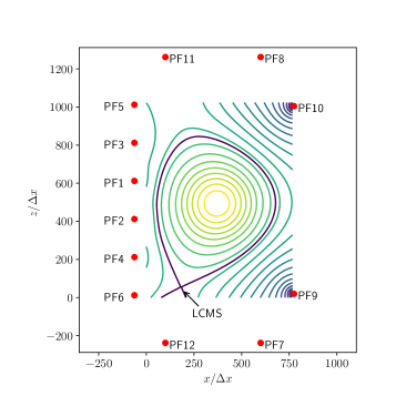
(a) Locations of PF coils and poloidal field lines.

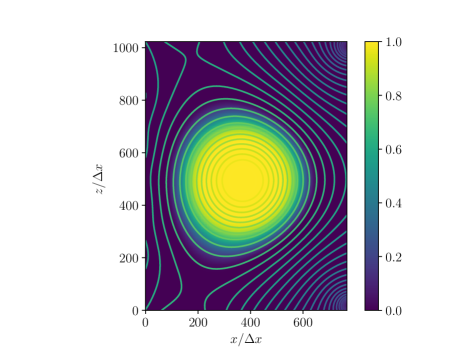
(b) Initial plasma density profile ($5\times 10^{19}\mathrm{m}^{-3})$.

Figure 1: Poloidal field and initial plasma density profile.

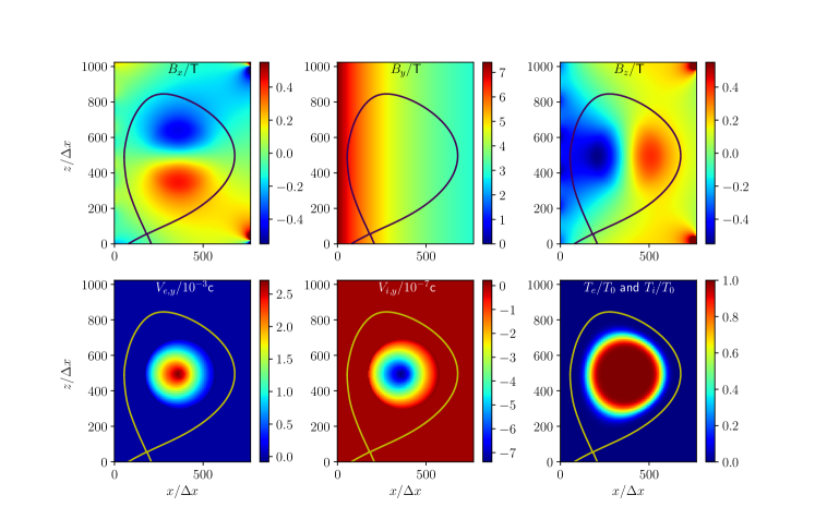
Figure 2: Tokamak external magnetic field and initial profiles of flow velocities in the $\mathbf{e}_{y}$ direction and temperatures.

At the beginning of the simulation, non-equilibrium distributions for deuterium ions and electrons are loaded into the device. The initial density profile in the poloidal plane is shown in Fig. 1(b). The 2D profiles of the external field and initial velocity and temperature profiles for both species are plotted in Fig. 2. Simulation parameters are chosen as

$$\Delta x = 8\times 10^{-4}\mathrm{m},\,\,\Delta t=0.1\Delta x/\mathrm{c},\,\,R_{0}=500\Delta x\leavevmode\nobreak\ ,$$

$$T_{e,0} = T_{i,0}=T_{0}=800\textrm{eV},\,\,n_{e,0}=n_{i,0}=5.0\times 10^{19}\mathrm{m}^{-3},$$

$$m_{i} = 3672m_{e}=3.34\times 10^{-27}\mathrm{kg},$$

$$J_{PF,i} = 67.9\mathrm{kA},\quad\textrm{for }1\leq i\leq 6\leavevmode\nobreak\ ,$$

$$J_{PF,7} = J_{PF,8}=211.1\mathrm{kA},\,\,J_{PF,9}=J_{PF,10}=238.1\mathrm{kA}\leavevmode\nobreak\ ,$$

$$J_{PF,11} = -189.9\mathrm{kA},\,\,J_{PF,12}=-211.1\mathrm{kA}\leavevmode\nobreak\ .$$

Detailed calculation of the external magnetic field, initial particle distributions, and boundary setup are outlined in Appendix A. Simulations show that the system reaches a steady state after $1.6\times 10^{7}$ time-steps. At this time, the amplitude of magnetic perturbation at the middle plane of the edge ($x=0.48$m and $z=0.41$m) is smaller than $B_{0}/200$, and the oscillation of position of plasma core is very small. Therefore, we can treat this state as a steady state. One such calculation requires about $1.3\times 10^{5}$ core-hours on the Tianhe 3 prototype cluster. Profiles of flow velocities, densities, temperatures of electrons and ions as well as electromagnetic field at the steady state are shown in Figs. 3-6.

Figure 3: Flow velocity distributions for electrons and ions at the steady state.

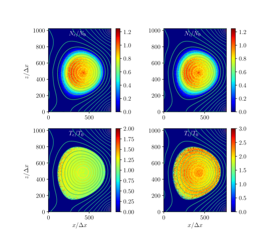
Figure 4: Density and temperature profiles of electrons and ions at the steady state.

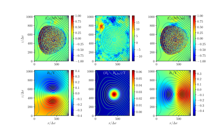
Figure 5: Electromagnetic field profiles at the steady state.

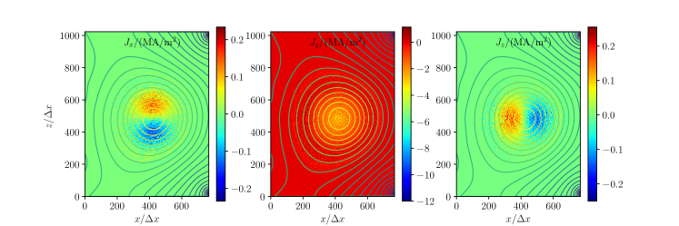
Figure 6: Current profiles at the steady state.

From Fig. 3, the flow velocity of ions at the steady state is in the range of $10$km/s, which is consistent with experimental observations (Ince-Cushman et al., 2009; Rice et al., 2009) and theoretical calculations (Guan et al., 2013a, b). This ion flow is much slower than the thermal velocity of ions and thus is negligible in the force balance for the steady state, which can be written as

$$\mathbf{j}\times\mathbf{B}-\nabla\cdot\bm{p}=0\leavevmode\nobreak\ .$$ (150)

Here, $\bm{p}$ is the pressure tensor. Equation (150) is obtained by the familiar procedure of taking the second moment of the Vlasov equation, subtracting the flow velocity and summing over species. From the simulation data, the $p_{ij}$ component of the pressure tensor is calculated as

$$p_{ij,J} =\sum_{\mathbf{x}_{sp}\in\textrm{grid }J}m_{s}v^{\prime}_{i,sp}v^{\prime}_{j,sp}\leavevmode\nobreak\ ,\quad\textrm{for }i,j\textrm{ in }\left\{x,y,z\right\}\leavevmode\nobreak\ ,$$ (151)

$$\mathbf{v}^{\prime}_{sp} \equiv\mathbf{v}_{sp}-\left(\sum_{\mathbf{x}_{sp}\in\textrm{grid }J}\mathbf{v}_{sp}\right)/\left(\sum_{\mathbf{x}_{sp}\in\textrm{grid }J}1\right)\leavevmode\nobreak\ .$$ (152)

The profile of pressure tensor at the steady state at $z=0.41$m is shown in Fig. 7. Clearly, the pressure tensor is predominately diagonal and anisotropic with $p_{yy}>p_{xx}\approx p_{zz}$. Note that the pressure is almost isotropic in the poloidal plane, which indicates that it is valid to adopt the ideal magnetohydrodynamics (MHD) model with a scalar pressure for force balance in the 2D tokamak equilibrium. However, for 3D physics, the effect of pressure anisotropy needs to be considered. Since the steady state is 2D in space for the present case, the force balance equation reduces to

$$\frac{\partial p_{xx}}{\partial x} =\left(\mathbf{j}\times\mathbf{B}\right)_{x}\,,$$ (153)

$$\frac{\partial p_{zz}}{\partial z} =\left(\mathbf{j}\times\mathbf{B}\right)_{z}\,.$$ (154)

To verify the force balance of the steady state, the four terms in Eqs. (153) and (154) are plotted in Fig. 8. For comparison, the components of $\partial p_{yy}/\partial x$ and $\partial p_{yy}/\partial z$ are also plotted. Figure 8 shows that the force balance is approximately satisfied for the numerically obtained steady state, which can be viewed as a self-consistent kinetic steady state.

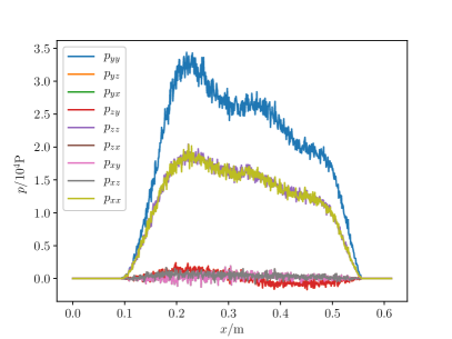
Figure 7: Pressure tensor profile at $z=0.41\mathrm{m}$.

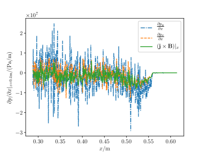
(a) $\mathbf{e}_{x}$ direction

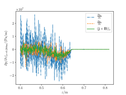
(b) $\mathbf{e}_{z}$ direction

Figure 8: Pressure gradient $\nabla\cdot\bm{p}$ and Lorentz force $\mathbf{j}\times\mathbf{B}$ in the $\mathbf{e}_{x}$ (a) and $\mathbf{e}_{z}$ (b) directions.

To verify the energy conservation in the simulation, we have recorded the time-history of the total energy in Fig. 9. The total energy drops a little, because some particles outside the last closed magnetic surface hit the simulation boundary, and these particles are removed from the simulation.

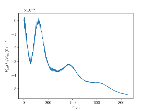
Figure 9: Evolution of total energy.

Before reaching the kinetic steady state, the plasma oscillates in the poloidal plane. It is expected that this oscillation can be described as an MHD process whose characteristic velocity is the Alfvén velocity $v_{A}=B_{0}/\sqrt{\mu_{0}n_{i}m_{i}}$. To observe this oscillation, we plot in Fig. 10 the evolution of the magnetic field at $x=600\Delta x$ and $z=512\Delta x$. From the parameters of the simulation, the characteristic frequency of the oscillation is

$$\omega_{A}=\frac{v_{A}}{qR_{0}}\sim 2.26\times 10^{-2}\omega_{c,i}\leavevmode\nobreak\ ,$$ (155)

which agrees with the frequency of the $B_{x}$ oscillation in Fig. 10.

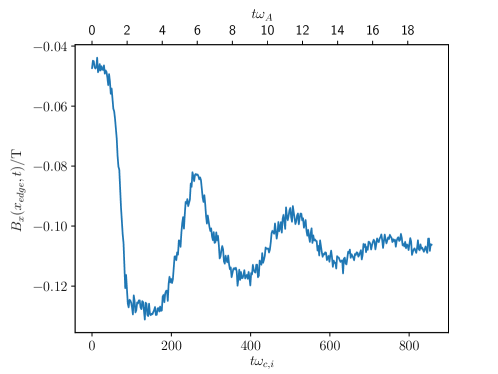
Figure 10: Evolution of $B_{x}(600\Delta x,0,512\Delta x)$.

III.2 Kinetic ballooning mode in tokamak

Kinetic Ballooning Mode (KBM) (Tang et al., 1980), characterized by both electromagnetic perturbations of the MHD type and nontrivial kinetic effects, plays an important role in tokamak edge physics. Traditionally, it has been simulated using electromagnetic gyrokinetic codes such as the Kin-2DEM (Qin, 1998; Qin et al., 1999a), LIGKA (Lauber et al., 2007), GTC (Zebin et al., 2013; Dong et al., 2019) and GEM (Wang et al., 2012). However, for edge plasmas, the gyrokinetic ordering (Hahm, 1988; Brizard, 1989; Qin et al., 1998, 1999b, 1999c, 2000a; Sugama, 2000; Qin and Tang, 2004; Qin, 2005; Qin et al., 2007; Burby et al., 2015; Burby, 2015; Burby and Brizard, 2019) may become invalid under certain parameter regimes for modern tokamaks. For instance, the characteristic length in the edge of the H-mode plasma simulated by Wan et al. (Wan et al., 2012, 2013) can be as short as about 5 times of the gyroradius of thermal ions, and in this situation, the gyrokinetic density calculation may be inaccurate. We have applied SymPIC code developed to carry out the first whole-device 6D kinetic simulations of the KBM in a tokamak geometry.

The machine parameters are the same as in Sec. III.1. To trigger the KBM instability, we increase the plasma density to $n_{0}=1\times 10^{20}\mathrm{m}^{-3}$, and the rest of parameters are

$$I_{p} = 0.858\mathrm{MA},\,\,T_{e,0}=T_{i,0}=T_{0}=800\textrm{eV}\leavevmode\nobreak\ ,$$

$$\Delta x = 3.2\times 10^{-3}\mathrm{m},\,\,\Delta t=0.5\Delta x/\mathrm{c}_{n},\,\,R_{0}=125\Delta x\leavevmode\nobreak\ ,$$

$$c_{n} = r_{c}\mathrm{c},\,\,m_{i}=r_{m}m_{e}=3.34\times 10^{-27}\mathrm{kg},$$

$$J_{PF,i} = 144.6\mathrm{kA},\quad\textrm{for }1\leq i\leq 6\leavevmode\nobreak\ ,$$

$$J_{PF,7} = J_{PF,8}=448.3\mathrm{kA},\,\,J_{PF,9}=J_{PF,10}=506.2\mathrm{kA}\leavevmode\nobreak\ ,$$

$$J_{PF,11} = -367.6\mathrm{kA},\,\,J_{PF,12}=-448.3\mathrm{kA}\leavevmode\nobreak\ .$$

Here $r_{m}$ is the mass ratio between the deuterium and electron, $c_{n}$ is the speed of light in the simulation and $r_{c}$ is the ratio between $c_{n}$ and the real speed of light in the vacuum $\mathrm{c}$. For real plasmas, $r_{m}\approx 3672$ and $r_{c}=1$. Limited by available computation power, we reduce $r_{m}$ and $r_{c}$ in some of the simulations. Such an approximation is valid because the low frequency ion motion is relatively independent from the mass of electron and the speed of light, as long as $r_{m}\gg 1$ and $\left(\mathrm{c}r_{c}/v_{A}\right)^{2}\gg 1.$ In the present work, we take $r_{m}=100$ and $r_{c}=0.16$ to obtain long-term simulation results. Short-term results for $r_{m}=300$, $r_{c}=0.5$ and $r_{m}=3672$, $r_{c}=1$ (in this case $\Delta t=0.1\Delta x/\mathrm{c}$) are also obtained for comparison. The simulation domain is a $192\times 64\times 256$ mesh, where perfect electric conductor is assumed at the boundaries in the $x$- and $z$-directions, and the periodic boundary is selected in $y$ direction.

Because of the steep pressure gradient in the edge of the plasma, the threshold $\beta_{\mathrm{crit}}$ for ballooning mode instability is low. An estimated scaling for $\beta_{\mathrm{crit}}$ is (Pueschel et al., 2008),

$$\beta_{\mathrm{crit}}=0.6\hat{s}/\left(\frac{2q^{2}R_{0}}{L_{p}}\right)\leavevmode\nobreak\ ,$$

where $\hat{s}$ is the magnetic shear and $L_{p}$ is the pressure scaling length. For our simulated plasma, $\beta_{\mathrm{crit}}\sim 1\times 10^{-3}$ and $\beta\approx 3\times 10^{-3}$. We except to observe unstable KBM.

To obtain a self-consistent kinetic steady state, we first perform a simulation as described in Sec. III.1 and obtain the 2D kinetic steady state. The profiles of temperature, safety factor, number density, pressure, toroidal current and bulk velocity of this steady state at $z=0.41$m are shown in Fig. 11.

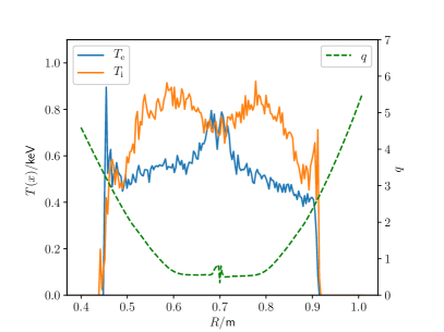
(a) Temperatures for electrons $T_{\mathrm{e}}$ and ions $T_{\mathrm{i}}$, and the safety factor $q$

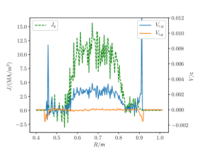
(b) Toroidal current $J_{\mathrm{y}}$, toroidal bulk velocities for electrons $V_{\mathrm{e,y}}$ and ions $V_{\mathrm{i,y}}$

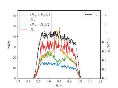
(c) Pressures for electrons $P_{\mathrm{e}}$ and ions $P_{\mathrm{i}}$, and the number density of electron, here for both electrons and ions it is found that $P_{i/e,x}\approx P_{i/e,z}$ so only $(P_{i/e,x}+P_{i/e,z})/2$ is plotted.

Figure 11: Profiles of the kinetic steady state at $z=0.41$m.

A random perturbation is then added in as the initial condition of the 6D simulation. The total simulation time is $t_{a}=1.5\times 10^{6}\Delta t\approx 10000\omega_{c,i}^{-1}\approx 5\times 10^{-5}$s. For one such simulation it takes about $3\times 10^{5}$ core-hours on the Tianhe 3 prototype cluster. The resulting mode structures of ion density for toroidal mode number $n=1,2,3,6,10,14,18$ are shown in Figs. 12, 13 and 14 for $t\omega_{c,i}=637,\,\,1241$ and $9693.$ It is clear that the unstable modes are triggered at the edge of the plasma, and the ballooning structure can be observed for modes with large $n$. The growth rate as a function of $n$ is plotted in Fig. 15. For comparison, the grow rate obtained using $r_{c}=0.5$, $r_{m}=300$ and $r_{c}=1$, $r_{m}=3672$ are also plotted. It is clear that the growth rate has little correlation with the reduction of $r_{c}$ and $r_{m}$. Figure 15 shows that the growth rate increases with $n,$ consistent with the early gyrokinetic simulation results obtained using the Kin-2DEM eigenvalue code (Qin, 1998; Qin et al., 1999a). Because the number of grids in the toroidal direction is 64 and the width of interpolating function is 4 times the grid size, the results for modes with $n>16$ may not be accurate. The results displayed here are thus preliminary. In the next step, we plan to perform a larger scale simulation with more realistic 2D equilibria to obtain improved accuracy.

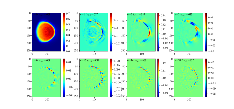
Figure 12: Mode structures of the electron density at $t=637/\omega_{c,i}=2.85a/v_{t,i}$.

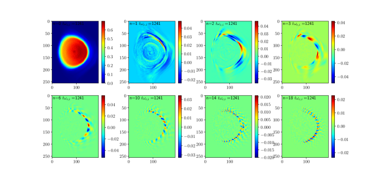
Figure 13: Mode structures of the electron density at $t=1241/\omega_{c,i}=5.55a/v_{t,i}$.

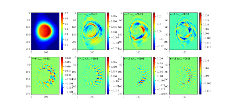
Figure 14: Mode structure of the electron density at $t=9693/\omega_{c,i}=43.35a/v_{t,i}$.

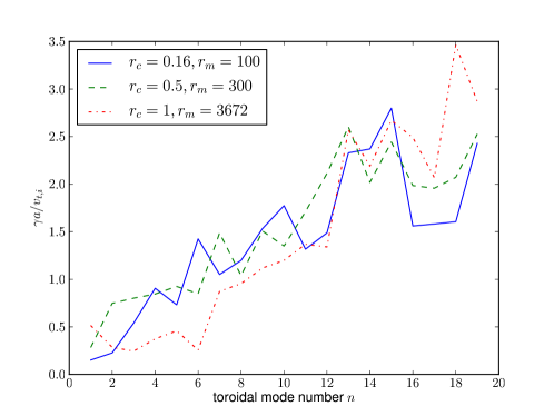
Figure 15: Growth rate as a function of toroidal mode number for different values of $r_{c}$ and $r_{m}$.

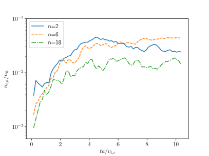
(a) Short-term evolution.

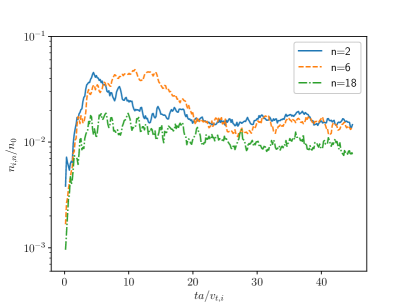
(b) Long-term evolution.

Figure 16: Time-history of ion densities for different toroidal mode number $n$.

The time-history of the mode amplitude is shown in Fig. 16. The unstable mode saturates approximately at $t\approx 5a/v_{t,i}$, and the saturation level is in the range of 2%. Recent nonlinear gyrokinetic simulation (Dong et al., 2019) suggested that the instability is saturated by the $E\times B$ zonal flow generated by the instability. To verify this mechanism in our 6D fully kinetic simulation, the toroidally averaged $\mathbf{E}$, $E\times B$ velocity and the measured phase velocity of the $n=12$ mode at $z=128\Delta x$ and $t=8a/v_{t,i}$ are compared in Fig. 17. The $E\times B$ velocity at the edge correlates strongly with the phase velocity of the perturbation in terms of amplitude and profile. As a result, the $E\times B$ flow for the background plasma generated by instability interacts coherently with the mode structure, significantly modifies the space-time structure of the perturbation relative to the background plasma and reduces the drive of the instability. For this case simulated, the nonlinear saturation mechanism agrees qualitatively with the nonlinear gyrokinetic simulation (Dong et al., 2019).

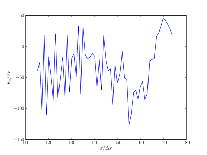
(a)

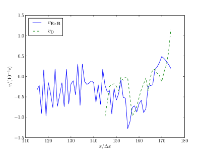
(b)

Figure 17: The toroidal averaged electric field in $\mathbf{e}_{x}$ direction (a). The $E\times B$ velocity $v_{E\times B}$ and measured phase velocity $v_{D}$ for the $n=12$ mode in the $\mathbf{e}_{z}$ direction at $z=128\Delta x$ and $t=8a/v_{t,i}$ (b) .

IV Conclusions

Even though 6D kinetic PIC method is a classical simulation tool for plasma physics, up to now it has not been applied to numerical studies of tokamak physics in spite of continuous improvement (Okuda, 1972; Cohen et al., 1982; Langdon et al., 1983; Cohen et al., 1989; Liewer and Decyk, 1989; Friedman et al., 1991; Eastwood, 1991; Cary and Doxas, 1993; Villasenor and Buneman, 1992; Qin et al., 2000b, c, 2001; Davidson and Qin, 2001; Esirkepov, 2001; Vay et al., 2002; Nieter and Cary, 2004; Huang et al., 2006; Crouseilles et al., 2007; Chen et al., 2011; Chacón et al., 2013; Evstatiev and Shadwick, 2013; Shadwick et al., 2014; Moon et al., 2015; Huang et al., 2016; Xiao and Qin, 2019b; Webb, 2016; Li et al., 2019, 2020; Holderied et al., 2020; Zheng et al., 2020a; Wang et al., 2020; Kormann and Sonnendrücker, 2021). In the present study, we have developed an explicit structure-preserving geometric PIC algorithm in curvilinear orthogonal meshes, in particular the cylindrical mesh, and apply it to carry out whole-device 6D kinetic simulation studies of tokamak physics. The work reported represents a further development of the structure-preserving geometric PIC algorithm (Squire et al., 2012a, b; Xiao et al., 2013, 2015a, 2015b; He et al., 2015a; Qin et al., 2016; He et al., 2016a; Kraus et al., 2017; Xiao et al., 2017, 2018; Xiao and Qin, 2019a), achieving the goal of practical applications in magnetic fusion research.

Along with it predecessors (Squire et al., 2012a, b; Xiao et al., 2013, 2015a, 2015b; He et al., 2015a; Qin et al., 2016; He et al., 2016a; Kraus et al., 2017; Xiao et al., 2017, 2018; Xiao and Qin, 2019a), the algorithm extends the symplectic integration method for finite dimensional canonical Hamiltonian systems developed since the 1980s (Devogelaere, 1956; Lee, 1983; Ruth, 1983; Feng, 1985, 1986; Lee, 1987; Sanz-Serna, 1988; Veselov, 1988; Yoshida, 1990; Forest and Ruth, 1990; Channell and Scovel, 1990; Candy and Rozmus, 1991; Tang, 1993; Sanz-Serna and Calvo, 1994; Shang, 1994; Kang and Zai-jiu, 1995; Shang, 1999; Marsden and West, 2001; Han-Ying et al., 2002; Hairer et al., 2002; Hong and Qin, 2002; jiu Shang, 2006; Feng and Qin, 2010; Zhang et al., 2016; Tao, 2016), and preserves an infinite dimensional non-canonical symplectic structure of the particle-field systems. In addition, other important geometric structures and conservation laws, such as the gauge symmetry, the local charge conservation law (Squire et al., 2012a, b; Xiao et al., 2018; Glasser and Qin, 2020) and the local energy conservation law (Xiao et al., 2017), are preserved exactly as well. These preserved structures and conservation laws improve the accuracy and fidelity of large-scale long-term simulations on modern computing hardware (Fu et al., 2016).

Through the whole-device 6D kinetic simulation, we numerically obtained a self-consistent kinetic steady state for fusion plasma in the tokamak geometry. It was found that the pressure tensor of the self-consistent kinetic steady state is diagonal, anisotropic in 3D, but isotropic in the poloidal plane. The steady state also includes a steady-state sub-sonic ion flow in the range of $10$km/s, which agrees with previous experimental observations (Ince-Cushman et al., 2009; Rice et al., 2009) and theoretical calculations (Guan et al., 2013a, b). Kinetic ballooning instability in the self-consistent kinetic steady state was successfully simulated. In the linear phase, it was found that high-$n$ ballooning modes have larger growth rates than low-$n$ global modes. In the nonlinear phase, the modes saturate approximately in $5$ ion transit times at the $2$% level by the $E\times B$ flow generated by the instability. These results qualitatively agrees with early (Qin, 1998; Qin et al., 1999a) and recent (Dong et al., 2019) simulations by electromagnetic gyrokinetic codes. In addition, compared with conventional gyrokinetic and reduced Braginskii Zeiler et al. (1997); Xu et al. (2010); Ricci et al. (2012) fluid simulation methods, more physical effects, such as fully kinetic dynamics and the self-consistent radial electric field, are naturally included in the present method. These effects can be crucial for edge plasmas and will be investigated in the next step.

It worth mentioning that in the present work we can not directly control the 2D kinetic steady state because it is numerically evolved from a given initial condition. In the future, we plan to solve this problem by adopting MHD equilibrium solutions as the initial conditions. Because a MHD equilibrium should be at least close to a lowest order kinetic steady state, it is expected that a kinetic steady state can be obtained by a short time evolution.

The present work can be also extended to describe more complex physical processes in tokamak plasmas. For example, we can add energetic particles to investigate their interactions with the background plasma. An antenna can be also modeled as a current source to study the wave heating and current drive (Zheng et al., 2020b). To simulate collision related physics, we can include Monte-Carlo Collision (MCC) (Birdsall, 1991) processes. It should be noted that due to the lack of marker particles in PIC simulations, the numerical collision frequency is usually larger than the real collision frequency of the plasma. More investigations are needed to determine the proper method to simulate collisions in the present scheme. Adding more physical effects to the geometric structure preserving PIC simulation framework will help us to better understand the tokamak physics. These topics will be addressed in the future study.

Appendix A External magnetic field of the tokamak, initial particle loading, and the boundary setup

In this appendix we describe the setup of external magnetic field of the tokamak, initial particle loading, and the boundary setup for the simulation study. The normalization of quantities are listed in Table 2.

Physical quantity	Symbol(s)	Unit
Length	$x,r,\dots$	$\Delta x$
Velocity	$\mathbf{v}$	$\mathrm{c}_{n}$
Mass	$m_{i}$	$m_{e}$
Time	$t$	$\Delta x/\mathrm{c}_{n}$

Table 2: Normalization for quantities.

The magnetic field is divided into three parts,

$$\mathbf{B}_{0,\textrm{init}}=\mathbf{B}_{0,p}+\mathbf{B}_{0,e}+\mathbf{B}_{0,t},$$ (156)

where $\mathbf{B}_{0,e}$ is the external magnetic fields generated by poloidal coils, $\mathbf{B}_{0,t}$ is the magnetic field generated by toloidal coils, i.e.,

$$\mathbf{B}_{0,t}=\frac{B_{0}R_{0}}{R}\thinspace,$$ (157)

and they do not evolve with time. $\mathbf{B}_{0,p}$ is the magnetic field generated by the plasma current. The current $\mathbf{j}$ and the vector potential $\mathbf{A}$ are related by

$$\nabla\times\left(\nabla\times\mathbf{A}\right) = \mathbf{j}\leavevmode\nobreak\ .$$ (158)

Initially, the current is in the $y$-direction and depends only on $x$ and $z$. In the adopted cylindrical coordinate $(x,y,z)$ the line element is

$$\mathrm{d}s^{2} = \left(\mathrm{d}x\right)^{2}+\left(\frac{x+R_{0}}{R_{0}}\mathrm{d}y\right)^{2}+\left(\mathrm{d}z\right)^{2}\leavevmode\nobreak\ ,$$ (159)

and Eq. (158) becomes

$$\frac{\partial^{2}}{\partial z^{2}}A_{y}\left(x,z\right)+\frac{\partial}{\partial x}\left(\frac{\partial}{\left(x+R_{0}\right)\partial x}\left(A_{y}\left(x,z\right)\left(x+R_{0}\right)\right)\right) = -j_{y}\left(x,z\right)\leavevmode\nobreak\ ,$$ (160)

$$\left(\frac{\partial^{2}}{\partial x^{2}}+\frac{\partial^{2}}{\partial z^{2}}\right)A_{y}^{o}\left(x,z\right)-\frac{1}{x+R_{0}}\frac{\partial}{\partial x}A_{y}^{o}\left(x,z\right) = -j_{y}^{o}\left(x,z\right)\leavevmode\nobreak\ ,$$ (161)

where

$$f^{o}(x,z)=f(x,z)\frac{x+R_{0}}{R_{0}}\leavevmode\nobreak\ .$$

When $j_{y}\left(x,z\right)=I_{0}\delta\left(x-x_{0}\right)\delta\left(z-z_{0}\right)$, which represents a coil current at $(x_{0},z_{0})$, Eq. (161) can be solved using spherical harmonic expansion. However the convergence of the series is slow when $r_{g}=\sqrt{\left(x+r_{0}\right)^{2}+(z-z_{0})^{2}}$ approaches $x_{0}+R_{0}$, the radius of the coil. We note that the second term in the left-hand-side of Eq. (161) is negligible when $R_{0}+x\gg B_{z}/\left(\partial B_{z}/\partial x\right)$. In this case, Eq. (161) simplifies to

$$\left(\frac{\partial^{2}}{\partial x^{2}}+\frac{\partial^{2}}{\partial z^{2}}\right)A_{y}^{o}\left(x,z\right) = -j_{y}^{o}\left(x,z\right)\leavevmode\nobreak\ ,$$ (162)

which is a standard 2D Poisson equation. Its solution for the coil current at $(x_{0},z_{0})$ with $I_{0}=1$ is

$$A_{y,PF}^{o}(x,z;x_{0},z_{0}) = \frac{1}{4\pi}\log\left(\left(x-x_{0}\right)^{2}+\left(z-z_{0}\right)^{2}\right)\leavevmode\nobreak\ .$$ (163)

Here, dimensionless variables have been used to simplify the notation. The total external vector potential generated by poloidal field coils is

$$A_{y,0,e}^{o}\left(x,z\right)=\sum_{i}J_{PF,i}A_{y,PF}^{o}\left(x,z;x_{PF,i},z_{PF,i}\right)\leavevmode\nobreak\ ,$$ (164)

where the locations of poloidal field coils are displayed in Tab. 3.

Coil number $i$	$x/$m	$z/$m	Coil number $i$	$x/$m	$z/$m
1	-0.05	0.4896	7	0.48	-0.1904
2	-0.05	0.3296	8	0.48	1.0096
3	-0.05	0.6496	9	0.62	0.0156
4	-0.05	0.1696	10	0.62	0.8036
5	-0.05	0.8096	11	0.08	1.0096
6	-0.05	0.0096	12	0.08	-0.1904

Table 3: Locations of tokamak poloidal field coils.

For $\mathbf{B}_{0,p}$ and the corresponding plasma current $\mathbf{j}_{0}$, we first construct a vector potential $\mathbf{A}_{y,0,p}$ and then use this potential to obtain $\mathbf{B}_{0,p}$ and $\mathbf{j}_{0}$. The constructed $A_{y,0,p}$ is

$$A_{y,0,p}^{o}\left(x,z\right)=\left\{\begin{array}[]{cc}-\frac{r^{2}B_{0}}{2q_{0}r_{0}}\leavevmode\nobreak\ ,&\textrm{ }r\leq r_{l}\,,\\ -\frac{B_{0}}{q_{0}r_{0}}\frac{9r^{2}r_{r}+6r_{l}^{3}\log(r_{l})+\left(-6\log(r)-5\right)r_{l}^{3}-4r^{3}}{18r_{r}-18r_{l}}\leavevmode\nobreak\ ,&r_{l}<r\leq r_{r}\,,\\ -\frac{B_{0}}{q_{0}r_{0}}\frac{6r_{r}^{3}\log(r_{r})+\log(r)\left(6r_{r}^{3}-6r_{l}^{3}\right)+5r_{r}^{3}+6r_{l}^{3}\log(r_{l})-5r_{l}^{3}}{18r_{r}-18r_{l}}\leavevmode\nobreak\ ,&\textrm{otherwise},\end{array}\right.\leavevmode\nobreak\$$

where $r=\sqrt{\left(x-x_{\mathrm{mid}}\right)^{2}+\left(z-z_{\mathrm{mid}}\right)^{2}}$, $x_{\mathrm{mid}}=N_{x}/2$ and $z_{\mathrm{mid}}=N_{z}/2$ are coordinates of the center of simulation domain, $q_{0}$ is the safety factor in the core of the plasma, $r_{l}=0.454a=0.1$m and $r_{r}=0.667a=0.147$m are two parameters that determine the current density distribution. The discrete magnetic fields are obtained by

$$\mathbf{B}_{J,0,p/e} = {\mathrm{curl_{d}}}\mathbf{A}_{0,p/e}\left(i,j,k\right)\leavevmode\nobreak\ ,$$ (165)

and the discrete current density is obtained from

$$\mathbf{j}_{J,0,\mathrm{all}} = {\mathrm{curl_{d}}^{T}}\left(\left(\mathbf{B}_{J,0,p}+\mathbf{B}_{J,0,e}\right)\left[\left(1+i/r_{0}\right)^{-1},1+i/r_{0},\left(1+i/r_{0}\right)^{-1}\right]\right)\leavevmode\nobreak\ .$$ (166)

The final plasma current is chosen as

$$\mathbf{j}_{J,0}=\left\{\begin{array}[]{cc}\mathbf{j}_{J,0,\mathrm{all}}\leavevmode\nobreak\ ,&\textrm{when }r<r_{r}\leavevmode\nobreak\ ,\\ 0\leavevmode\nobreak\ ,&\textrm{otherwise.}\end{array}\right.\leavevmode\nobreak\$$ (169)

Density and temperature are calculated from $A_{y,0}^{o}=A_{y,0,e}^{o}+A_{y,0,p}^{o}$. We introduce a reference function $g_{r}$ defined as

$$g_{r}(x,z)=1-\left\{\begin{array}[]{cc}0\leavevmode\nobreak\ ,&A_{y,0}^{o}\left(x,z\right)<A_{y,\min}^{o}\,,\\ \frac{A_{y,0}^{o}\left(x,z\right)-A_{y,\min}^{o}}{A_{y,\max}^{o}-A_{y,\min}^{o}}\leavevmode\nobreak\ ,&A_{y,\min}^{o}\leq A_{y,0}^{o}\left(x,z\right)<A_{y,\max}^{o}\,,\\ 1\leavevmode\nobreak\ ,&A_{y,\max}^{o}\leq A_{y,0}^{o}\,,\end{array}\right.$$ (170)

where

$$A_{y,\min}^{o} = A_{y,0}^{o}\left(0.267N_{x},0.114N_{z}\right)\leavevmode\nobreak\ ,$$ (171)

$$A_{y,\max}^{o} = A_{y,0}^{o}\left(0.488N_{x},0.369N_{z}\right)\leavevmode\nobreak\ .$$ (172)

The initial density and temperature for electrons and ions are

$$n_{e}=n_{i} = n_{e,0}\left(\left(g_{r}\left(x,z\right)^{2}+1\right)\left(1-g_{r}\left(x,z\right)^{2}\right)\right)^{3}\leavevmode\nobreak\ ,$$ (173)

$$T_{e}=T_{i} = T_{e,0}\left(\left(g_{r}\left(x,z\right)^{2}+1\right)\left(1-g_{r}\left(x,z\right)^{2}\right)\right)^{6}\leavevmode\nobreak\ .$$ (174)

In this work, ions are all deuterium ions, and the initial velocity distribution for each specie is Maxwellian with a flow velocity, i.e.,

$$f_{e/i,0}\left(\mathbf{x},\mathbf{v}\right) = \frac{n_{e/i}\left(x,z\right)}{\left(2\pi T_{e/i}/m_{e/i}\right)^{3/2}}\exp\left(-\frac{|\mathbf{v}+v_{e/i,y,0}\left(x,z\right)\mathbf{e}_{y}|^{2}}{2T_{e/i}/m_{e/i}}\right)\leavevmode\nobreak\ ,$$ (175)

where

$$v_{e/i,y,0}\left(x,z\right)=\frac{j_{y,0}\left(x,z\right)m_{i/e}}{q_{e/i}\left(m_{i}-m_{e}\right)n_{e/i}\left(x,z\right)}\leavevmode\nobreak\ .$$ (176)

The boundaries of the simulations are configured as follows. The boundaries at $x=0$, $x=N_{x}\Delta x$, $z=0$, and $z=N_{z}\Delta z$ are chosen to be perfect electric conductors for the electromagnetic fields. For particles, we introduce a thin slow-down layer,

$$\mathbf{L}_{\mathrm{p}}= \big{\{}\left(x,y,z\right)|0<x<5\Delta x\quad\textrm{or}\quad 0<z<5\Delta z\quad\textrm{or}$$

$$\left(N_{x}-5\right)\Delta x<x<N_{x}\Delta x\quad\textrm{or}\quad\left(N_{z}-5\right)\Delta z<z<N_{z}\Delta z\Big{\}}\leavevmode\nobreak\ .$$

If a particle is inside $\mathbf{\mathbf{L}_{\mathrm{p}}}$ at a time-step, its velocity $\mathbf{v}_{p}$ will be reduced to $0.98\mathbf{v}_{p}$ at the end of this time-step, and the particle will be removed when $\mathbf{v}_{p}$ is smaller than $1\times 10^{-5}\mathrm{c}$. Periodic boundaries for both particles and electromagnetic fields are adopted in the $y$-direction. The plasma is confined inside the last closed flux surface mostly, and the shape of plasma is not directly related to the simulation boundaries.

Appendix B Explicit 2nd-order structure-preserving geometric PIC algorithm in the cylindrical mesh

In this appendix, we list the detailed update rule for the 2nd-order structure-preserving geometric PIC algorithm in the cylindrical mesh introduced in Sec. II.5. It updates previous particle locations and discrete electromagnetic fields $\{\mathbf{x}_{sp,2l-2},\mathbf{x}_{sp,2l-1},\mathbf{E}_{J,l},\mathbf{B}_{K,l}\}$ to the current ones $\{\mathbf{x}_{sp,2l},\mathbf{x}_{sp,2l+1},\mathbf{E}_{J,l+1},\mathbf{B}_{K,l+1}\}$,

$$x_{sp,2l} = 2x_{sp,2l-1}-x_{sp,2l-2}+\Delta x^{-2}\left(2\frac{q_{s}}{m_{s}}h^{2}E_{x,1}\right)\leavevmode\nobreak\ ,$$

$$y_{sp,2l} = \left(r_{0}^{2}+2r_{0}x_{sp,2l}+x_{sp,2l}^{2}\right)^{-1}\left(\left(-2r_{0}x_{sp,2l-2}-r_{0}^{2}-x_{sp,2l-2}^{2}\right)y_{sp,2l-2}+\right.$$

$$\left.\left(2r_{0}^{2}+2r_{0}x_{sp,2l-2}+x_{sp,2l-2}^{2}+2r_{0}x_{sp,2l}+x_{sp,2l}^{2}\right)y_{sp,2l-1}\right)+$$

$$r_{0}^{2}\left(\frac{q_{s}}{m_{s}}h\left(2E_{y,1}h-\left(B_{z,0,0,1,1,0}+B_{z,1,1,1,1,0}\right)\right)\right)\left(\Delta y^{2}r_{0}^{2}+2\Delta y^{2}r_{0}x_{sp,2l}+\Delta y^{2}x_{sp,2l}^{2}\right)^{-1}\leavevmode\nobreak\ ,$$

$$z_{sp,2l} = 2z_{sp,2l-1}-z_{sp,2l-2}+$$

$$\Delta z^{-2}\left(\frac{q_{s}}{m_{s}}h\left(2E_{z,1}h+\left(B_{y,0,0,1,1,0}-B_{x,0,0,0,1,1}-B_{x,1,2,1,1,1}+B_{y,1,1,1,1,0}\right)\right)\right)\leavevmode\nobreak\ ,$$

$$z_{sp,2l+1} = 2z_{sp,2l}-z_{sp,2l-1}\leavevmode\nobreak\ ,$$

$$y_{sp,2l+1} = 2y_{sp,2l}-y_{sp,2l-1}+r_{0}^{2}\left(h\frac{q_{s}}{m_{s}}\left(B_{x,1,2,2,2,2}+B_{x,1,2,2,1,2}\right)\right)\left(\Delta y^{2}r_{0}^{2}+2\Delta y^{2}r_{0}x_{sp,2l}+\Delta y^{2}x_{sp,2l}^{2}\right)^{-1}$$

$$x_{sp,2l+1} = \Delta x^{-2}r_{0}^{-2}\left(-\Delta x^{2}r_{0}^{2}x_{sp,2l-1}+2\Delta x^{2}r_{0}^{2}x_{sp,2l}+\left(\Delta y^{2}r_{0}+\Delta y^{2}x_{sp,2l}\right)y_{sp,2l-1}^{2}\right.$$

$$\left.+\left(-2\Delta y^{2}r_{0}-2\Delta y^{2}x_{sp,2l}\right)y_{sp,2l-1}y_{sp,2l}+\left(2\Delta y^{2}r_{0}+2\Delta y^{2}x_{sp,2l}\right)y_{sp,2l}^{2}\right.$$

$$\left.+\left(-2\Delta y^{2}r_{0}-2\Delta y^{2}x_{sp,2l}\right)y_{sp,2l}y_{sp,2l+1}+\left(\Delta y^{2}r_{0}+\Delta y^{2}x_{sp,2l}\right)y_{sp,2l+1}^{2}\right)\leavevmode\nobreak\ ,$$

$$+\Delta x^{-2}\left(-h\frac{q_{s}}{m_{s}}\left(B_{y,1,2,2,1,2}+B_{y,1,2,2,2,2}-B_{z,1,2,1,1,1}-B_{z,1,2,2,3,1}\right)\right)\leavevmode\nobreak\ ,$$

$$\frac{1}{\mathbf{h}_{\sigma 1}\left(\mathbf{x}_{J}\right)\mathbf{h}_{\sigma 1}\left(\mathbf{x}_{J}\right)}\frac{\mathbf{E}_{J,l+1}-\mathbf{E}_{J,l}}{\Delta t}h_{\sigma 3}\left(\mathbf{x}_{J}\right) = \sum_{K}{\mathrm{curl_{d}}^{T}}_{J,K}\frac{h_{\sigma 3}\left(\mathbf{x}_{J}\right)}{\mathbf{h}_{\sigma 2}\left(\mathbf{x}_{K}\right)\mathbf{h}_{\sigma 2}\left(\mathbf{x}_{K}\right)}\mathbf{B}_{K,l}-\mathbf{j}_{J,l}\leavevmode\nobreak\ ,$$

$$\frac{\mathbf{B}_{K,l+1}-\mathbf{B}_{K,l}}{\Delta t} = -\sum_{J}{\mathrm{curl_{d}}}_{K,J}\mathbf{E}_{J,l+1}\leavevmode\nobreak\ ,$$

where

$$h = \Delta t/2\leavevmode\nobreak\ ,$$

$$\mathbf{B}_{t,i_{1},i_{2},i_{3},i_{4}} = \left[\begin{array}[]{c}B_{x,t,i_{1},i_{2},i_{3},i_{4}}\\ B_{y,t,i_{1},i_{2},i_{3},i_{4}}\\ B_{z,t,i_{1},i_{2},i_{3},i_{4}}\end{array}\right]=\int_{x_{i_{4}+1,sp,2l+i_{i_{4}+1}}}^{x_{i_{4}+1,sp,2l+i_{i_{4}+1}+1}}\mathrm{d}\bar{x}\sum_{J}\mathbf{B}_{J,l+t-1}$$

$$W_{\sigma_{2}J}\left(\left[x_{sp,2l+i_{1}},y_{sp,2l+i_{2}},z_{sp,2l+i_{3}}\right]+\mathbf{e}_{x_{i_{4}+1}}\left(\bar{x}-x_{i_{4}+1,sp,2l+i_{i_{4}+1}}\right)\right)\leavevmode\nobreak\ ,$$

$$\mathbf{E}_{1} = \left[\begin{array}[]{c}E_{x,1}\\ E_{y,1}\\ E_{z,1}\end{array}\right]=\sum_{J}\mathbf{E}_{J,l}W_{\sigma_{1}J}\left(\mathbf{x}_{sp,2l-1}\right)\leavevmode\nobreak\ ,$$

$$\mathbf{j}_{J,l} = \frac{1}{\Delta t}\sum_{s,p}q_{s}\int_{C_{sp,2l-1,2l}\bigcup C_{sp,2l,2l+1}^{*}}W_{\sigma_{1}J}\left(\mathbf{x}\right)\mathrm{d}\mathbf{x}\leavevmode\nobreak\ ,$$

$$C_{sp,2l-1,2l} = \left\{\left(x_{1,sp2l-1}+\tau\left(x_{1,sp,2l}-x_{1,sp2l-1}\right),x_{2,sp2l-1},x_{3,sp2l-1}\right)|\tau\in\left[0,1\right)\right\}\bigcup$$

$$\left\{\left(x_{1,sp,2l},x_{2,sp2l-1}+\tau\left(x_{2,sp,2l}-x_{2,sp2l-1}\right),x_{3,sp2l-1}\right)|\tau\in\left[0,1\right)\right\}\bigcup$$

$$\left\{\left(x_{1,sp,2l},x_{2,sp,2l},x_{3,sp2l-1}+\tau\left(x_{3,sp,2l}-x_{3,sp2l-1}\right)\right)|\tau\in\left[0,1\right)\right\}\leavevmode\nobreak\ ,$$

$$C_{sp,2l,2l+1}^{*} = \left\{\left(x_{1,sp,2l}+\tau\left(x_{1,sp,2l+1}-x_{1,sp,2l}\right),x_{2,sp,2l+1},x_{3,sp,2l+1}\right)|\tau\in\left[0,1\right)\right\}\bigcup$$

$$\left\{\left(x_{1,sp,2l},x_{2,sp,2l}+\tau\left(x_{2,sp,2l+1}-x_{2,sp,2l}\right),x_{3,sp,2l+1}\right)|\tau\in\left[0,1\right)\right\}\bigcup$$

$$\left\{\left(x_{1,sp,2l},x_{2,sp,2l},x_{3,sp,2l}+\tau\left(x_{3,sp,2l+1}-x_{3,sp,2l}\right)\right)|\tau\in\left[0,1\right)\right\}\leavevmode\nobreak\ .$$

References

- Squire et al. (2012a) J. Squire, H. Qin, and W. M. Tang, Geometric Integration of the Vlasov-Maxwell System with a Variational Particle-in-cell Scheme, Tech. Rep. PPPL-4748 (Princeton Plasma Physics Laboratory, 2012).
- Squire et al. (2012b) J. Squire, H. Qin, and W. M. Tang, Physics of Plasmas 19, 084501 (2012b).
- Xiao et al. (2013) J. Xiao, J. Liu, H. Qin, and Z. Yu, Physics of Plasmas 20, 102517 (2013).
- Xiao et al. (2015a) J. Xiao, H. Qin, J. Liu, Y. He, R. Zhang, and Y. Sun, Physics of Plasmas 22, 112504 (2015a).
- Xiao et al. (2015b) J. Xiao, J. Liu, H. Qin, Z. Yu, and N. Xiang, Physics of Plasmas 22, 092305 (2015b).
- He et al. (2015a) Y. He, H. Qin, Y. Sun, J. Xiao, R. Zhang, and J. Liu, Physics of Plasmas (1994-present) 22, 124503 (2015a).
- Qin et al. (2016) H. Qin, J. Liu, J. Xiao, R. Zhang, Y. He, Y. Wang, Y. Sun, J. W. Burby, L. Ellison, and Y. Zhou, Nuclear Fusion 56, 014001 (2016).
- He et al. (2016a) Y. He, Y. Sun, H. Qin, and J. Liu, Physics of Plasmas 23, 092108 (2016a).
- Kraus et al. (2017) M. Kraus, K. Kormann, P. J. Morrison, and E. Sonnendrücker, Journal of Plasma Physics 83, 905830401 (2017).
- Xiao et al. (2017) J. Xiao, H. Qin, J. Liu, and R. Zhang, Physics of Plasmas 24, 062112 (2017).
- Xiao et al. (2018) J. Xiao, H. Qin, and J. Liu, Plasma Science and Technology 20, 110501 (2018).
- Xiao and Qin (2019a) J. Xiao and H. Qin, Nuclear Fusion 59, 106044 (2019a).
- Ince-Cushman et al. (2009) A. Ince-Cushman, J. E. Rice, M. Reinke, M. Greenwald, G. Wallace, R. Parker, C. Fiore, J. W. Hughes, P. Bonoli, S. Shiraiwa, A. Hubbard, S. Wolfe, I. H. Hutchinson, E. Marmar, M. Bitter, J. Wilson, and K. Hill, Physical Review Letters 102, 035002 (2009).
- Rice et al. (2009) J. Rice, A. Ince-Cushman, P. Bonoli, M. Greenwald, J. Hughes, R. Parker, M. Reinke, G. Wallace, C. Fiore, R. Granetz, A. Hubbard, J. Irby, E. Marmar, S. Shiraiwa, S. Wolfe, S. Wukitch, M. Bitter, K. Hill, and J. Wilson, Nuclear Fusion 49, 025004 (2009).
- Guan et al. (2013a) X. Guan, I. Y. Dodin, H. Qin, J. Liu, and N. J. Fisch, Physics of Plasmas 20, 102105 (2013a).
- Guan et al. (2013b) X. Guan, H. Qin, J. Liu, and N. J. Fisch, Physics of Plasmas 20, 022502 (2013b).
- Qin (1998) H. Qin, Gyrokinetic Theory and Computational Methods for Electromagnetic Perturbationsin Tokamaks, Ph.D. thesis, Princeton University, Princeton, NJ 08540 (1998).
- Qin et al. (1999a) H. Qin, W. M. Tang, and G. Rewoldt, Physics of Plasmas 6, 2544 (1999a).
- Dong et al. (2019) G. Dong, J. Bao, A. Bhattacharjee, and Z. Lin, Physics of Plasmas 26, 010701 (2019).
- Dawson (1983) J. M. Dawson, Reviews of Modern Physics 55, 403 (1983).
- Hockney and Eastwood (1988) R. W. Hockney and J. W. Eastwood, Computer Simulation Using Particles (CRC Press, 1988).
- Birdsall and Langdon (1991) C. K. Birdsall and A. B. Langdon, Plasma Physics via Computer Simulation (IOP Publishing, 1991) p. 293.
- Yee et al. (1966) K. S. Yee et al., IEEE Trans. Antennas Propag 14, 302 (1966).
- Boris (1970) J. Boris, in Proceedings of the Fourth Conference on Numerical Simulation of Plasmas (Naval Research Laboratory, Washington D. C., 1970) p. 3.
- Stern et al. (2015) A. Stern, Y. Tong, M. Desbrun, and J. E. Marsden, in Geometry, Mechanics, and Dynamics (Springer, 2015) pp. 437–475.
- Qin et al. (2013) H. Qin, S. Zhang, J. Xiao, J. Liu, Y. Sun, and W. M. Tang, Physics of Plasmas (1994-present) 20, 084503 (2013).
- He et al. (2015b) Y. He, Y. Sun, J. Liu, and H. Qin, Journal of Computational Physics 281, 135 (2015b).
- Zhang et al. (2015) R. Zhang, J. Liu, H. Qin, Y. Wang, Y. He, and Y. Sun, Physics of Plasmas (1994-present) 22, 044501 (2015).
- Ellison et al. (2015a) C. Ellison, J. Burby, and H. Qin, Journal of Computational Physics 301, 489 (2015a).
- He et al. (2016b) Y. He, Y. Sun, J. Liu, and H. Qin, Journal of Computational Physics 305, 172 (2016b).
- Tu et al. (2016) X. Tu, B. Zhu, Y. Tang, H. Qin, J. Liu, and R. Zhang, Physics of Plasmas 23, 122514 (2016).
- Ueda et al. (1994) H. Ueda, Y. Omura, H. Matsumoto, and T. Okuzawa, Computer physics communications 79, 249 (1994).
- Fu et al. (2016) H. Fu, J. Liao, J. Yang, L. Wang, Z. Song, X. Huang, C. Yang, W. Xue, F. Liu, F. Qiao, et al., Science China Information Sciences 59, 072001 (2016).
- Morrison (2017) P. J. Morrison, Physics of Plasmas 24, 055502 (2017).
- Holderied et al. (2020) F. Holderied, S. Possanner, A. Ratnani, and X. Wang, Journal of Computational Physics 402, 109108 (2020).
- Xiao and Qin (2019b) J. Xiao and H. Qin, “Structure-preserving geometric particle-in-cell algorithm suppresses finite-grid instability – comment on ”Finite grid instability and spectral fidelity of the electrostatic particle-in-cell algorithm” by Huang et al.” (2019b), arXiv:1904.00535v1 .
- Li et al. (2019) Y. Li, Y. He, Y. Sun, J. Niesen, H. Qin, and J. Liu, Journal of Computational Physics 396, 381 (2019).
- Li et al. (2020) Y. Li, Y. Sun, and N. Crouseilles, Journal of Computational Physics 405, 109172 (2020).
- Hirvijoki et al. (2020) E. Hirvijoki, K. Kormann, and F. Zonta, “Subcycling of particle orbits in variational, geometric electromagnetic particle-in-cell methods,” (2020), arXiv:2002.10759v2 .
- Perse et al. (2020) B. Perse, K. Kormann, and E. Sonnendrücker, “Geometric particle-in-cell simulations of the vlasov–maxwell system in curvilinear coordinates,” (2020), arXiv:2002.09386v1 .
- Zheng et al. (2020a) J. Zheng, J. Chen, F. Lu, J. Xiao, H. An, and L. Shen, Plasma Physics and Controlled Fusion 62, 125020 (2020a).
- Wang et al. (2020) Z. Wang, H. Qin, B. Sturdevant, and C.-S. Chang, “Geometric electrostatic particle-in-cell algorithm on unstructured meshes,” (2020), arXiv:2012.08587 [physics.plasm-ph] .
- Kormann and Sonnendrücker (2021) K. Kormann and E. Sonnendrücker, Journal of Computational Physics 425, 109890 (2021).
- Lin et al. (1998) Z. Lin, T. S. Hahm, W. Lee, W. M. Tang, and R. B. White, Science 281, 1835 (1998).
- Zebin et al. (2013) L. Zebin, S. Guoya, I. Holod, X. Yong, Z. Wenlu, and L. Zhihong, Plasma Science and Technology 15, 499 (2013).
- Ku et al. (2006) S. Ku, C.-S. Chang, M. Adams, J. Cummings, F. Hinton, D. Keyes, S. Klasky, W. Lee, Z. Lin, S. Parker, et al., Journal of Physics: Conference Series 46, 87 (2006).
- Chang et al. (2009) C.-S. Chang, S. Ku, P. Diamond, Z. Lin, S. Parker, T. Hahm, and N. Samatova, Physics of Plasmas 16, 056108 (2009).
- Chen and Parker (2003) Y. Chen and S. E. Parker, Journal of Computational Physics 189, 463 (2003).
- Chen and Parker (2007) Y. Chen and S. E. Parker, Journal of Computational Physics 220, 839 (2007).
- Wang et al. (2012) E. Wang, X. Xu, J. Candy, R. Groebner, P. Snyder, Y. Chen, S. Parker, W. Wan, G. Lu, and J. Dong, Nuclear Fusion 52, 103015 (2012).
- Lee (1983) T. Lee, Phys. Lett. B 122, 217 (1983).
- Lee (1987) T. Lee, J. Statis. Phys. 46, 843 (1987).
- Veselov (1988) A. P. Veselov, Funkc. Anal. Priloz. 22, 1 (1988).
- Marsden and West (2001) J. E. Marsden and M. West, Acta Numer. 10, 357 (2001).
- Han-Ying et al. (2002) G. Han-Ying, L. Yu-Qi, W. Ke, and W. Shi-Kun, Communications in Theoretical Physics 37, 257 (2002).
- Qin (2020) H. Qin, Scientific Reports 10, 19329 (2020).
- Hutchinson et al. (1994) I. Hutchinson, R. Boivin, F. Bombarda, P. Bonoli, S. Fairfax, C. Fiore, J. Goetz, S. Golovato, R. Granetz, M. Greenwald, et al., Physics of Plasmas 1, 1511 (1994).
- Greenwald et al. (1997) M. Greenwald, R. Boivin, F. Bombarda, P. Bonoli, C. Fiore, D. Garnier, J. Goetz, S. Golovato, M. Graf, R. Granetz, et al., Nuclear Fusion 37, 793 (1997).
- Xiao et al. (2016) J. Xiao, H. Qin, P. J. Morrison, J. Liu, Z. Yu, R. Zhang, and Y. He, Physics of Plasmas (1994-present) 23, 112107 (2016).
- Zhou et al. (2014) Y. Zhou, H. Qin, J. Burby, and A. Bhattacharjee, Physics of Plasmas (1994-present) 21, 102109 (2014).
- Zhou et al. (2016) Y. Zhou, Y.-M. Huang, H. Qin, and A. Bhattacharjee, Phys. Rev. E 93, 023205 (2016).
- Zhou (2017) Y. Zhou, Variational Integration for Ideal Magnetohydrodynamics and Formation of Current Singularities, Ph.D. thesis, Princeton University (2017).
- Zhou et al. (2017a) Y. Zhou, Y.-M. Huang, H. Qin, and A. Bhattacharjee, The Astrophysical Journal 852, 3 (2017a).
- Burby and Tronci (2017) J. W. Burby and C. Tronci, Plasma Physics and Controlled Fusion 59, 045013 (2017).
- Chen et al. (2017) Q. Chen, H. Qin, J. Liu, J. Xiao, R. Zhang, Y. He, and Y. Wang, Journal of Computational Physics 349, 441 (2017).
- Shi et al. (2016) Y. Shi, N. J. Fisch, and H. Qin, Physical Review A 94, 012124 (2016).
- Shi et al. (2018) Y. Shi, J. Xiao, H. Qin, and N. J. Fisch, Physical Review E 97, 053206 (2018).
- Shi (2018) Y. Shi, Plasma Physics in Strong Field Regimes, Ph.D. thesis, Princeton University (2018).
- Shi et al. (2020) Y. Shi, H. Qin, and N. J. Fisch, “Plasma physics in strong-field regimes: theories and simulations,” (2020), arXiv:2012.15363 [physics.plasm-ph] .
- Chen and Xiao (2019) Q. Chen and J. Xiao, “Gauge and Poincaré invariant canonical symplectic algorithms for real-time lattice strong-field quantum electrodynamics,” (2019), arXiv:1910.09215v2 .
- Hirvijoki et al. (2018) E. Hirvijoki, M. Kraus, and J. W. Burby, “Metriplectic particle-in-cell integrators for the landau collision operator,” (2018), arXiv:1802.05263 .
- Hirani (2003) A. N. Hirani, Discrete Exterior Calculus, Ph.D. thesis, California Institute of Technology (2003).
- Desbrun et al. (2005) M. Desbrun, A. N. Hirani, M. Leok, and J. E. Marsden, “Discrete exterior calculus,” (2005), arXiv:math/0508341 .
- Whitney (1957) H. Whitney, Geometric Integration Theory (Princeton University Press, 1957).
- Morrison (1980) P. J. Morrison, Physics Letters A 80, 383 (1980).
- Marsden and Weinstein (1982) J. E. Marsden and A. Weinstein, Physica D: Nonlinear Phenomena 4, 394 (1982).
- Weinstein and Morrison (1981) A. Weinstein and P. J. Morrison, Physics Letters A 86, 235 (1981).
- Burby (2017) J. W. Burby, Physics of Plasmas 24, 032101 (2017).
- Iwinski and Turski (1976) Z. R. Iwinski and L. A. Turski, Letters in Applied and Engineering Sciences 4, 179 (1976).
- Devogelaere (1956) R. Devogelaere, Methods of Integration Which Preserve the Contact Transformation Property of the Hamilton Equations, Tech. Rep. (University of Notre Dame, 1956).
- Ruth (1983) R. D. Ruth, IEEE Trans. Nucl. Sci 30, 2669 (1983).
- Feng (1985) K. Feng, in the Proceedings of 1984 Beijing Symposium on Differential Geometry and Differential Equations, edited by K. Feng (Science Press, 1985) pp. 42–58.
- Feng (1986) K. Feng, J. Comput. Maths. 4, 279 (1986).
- Sanz-Serna (1988) J. M. Sanz-Serna, BIT 28, 877 (1988).
- Yoshida (1990) H. Yoshida, Physics Letters A 150, 262 (1990).
- Forest and Ruth (1990) E. Forest and R. D. Ruth, Physica D 43, 105 (1990).
- Channell and Scovel (1990) P. J. Channell and C. Scovel, Nonlinearity 3, 231 (1990).
- Candy and Rozmus (1991) J. Candy and W. Rozmus, Journal of Computational Physics 92, 230 (1991).
- Tang (1993) Y.-F. Tang, Computers & Mathematics with Applications 25, 83 (1993).
- Sanz-Serna and Calvo (1994) J. M. Sanz-Serna and M. P. Calvo, Numerical Hamiltonian Problems (Chapman and Hall, London, 1994).
- Shang (1994) Z. Shang, Journal of Computational Mathematics 2, 265 (1994).
- Kang and Zai-jiu (1995) F. Kang and S. Zai-jiu, Numerische Mathematik 71, 451 (1995).
- Shang (1999) Z. Shang, Numerische Mathematik 83, 477 (1999).
- Hairer et al. (2002) E. Hairer, C. Lubich, and G. Wanner, Geometric Numerical Integration: Structure-Preserving Algorithms for Ordinary Differential Equations (Springer, New York, 2002).
- Hong and Qin (2002) J. Hong and M. Z. Qin, Applied Mathematics Letters 15, 1005 (2002).
- jiu Shang (2006) Z. jiu Shang, Journal of Physics A: Mathematical and General 39, 5601 (2006).
- Feng and Qin (2010) K. Feng and M. Qin, Symplectic Geometric Algorithms for Hamiltonian Systems (Springer-Verlag, 2010).
- Zhang et al. (2016) R. Zhang, H. Qin, Y. Tang, J. Liu, Y. He, and J. Xiao, Physical Review E 94, 013205 (2016).
- Tao (2016) M. Tao, Journal of Computational Physics 327, 245 (2016).
- Qin and Guan (2008) H. Qin and X. Guan, Physical Review Letters 100, 035006 (2008).
- Qin et al. (2009) H. Qin, X. Guan, and W. M. Tang, Physics of Plasmas (1994-present) 16, 042510 (2009).
- Squire et al. (2012c) J. Squire, H. Qin, and W. M. Tang, Physics of Plasmas 19, 052501 (2012c).
- Zhang et al. (2014) R. Zhang, J. Liu, Y. Tang, H. Qin, J. Xiao, and B. Zhu, Physics of Plasmas (1994-present) 21, 032504 (2014).
- Ellison et al. (2015b) C. L. Ellison, J. M. Finn, H. Qin, and W. M. Tang, Plasma Physics and Controlled Fusion 57, 054007 (2015b).
- Burby and Ellison (2017) J. Burby and C. Ellison, Physics of Plasmas 24, 110703 (2017).
- Kraus (2017) M. Kraus, “Projected variational integrators for degenerate lagrangian systems,” (2017), arXiv:1708.07356v1 .
- Ellison et al. (2018) C. L. Ellison, J. M. Finn, J. W. Burby, M. Kraus, H. Qin, and W. M. Tang, Physics of Plasmas 25, 052502 (2018).
- Ellison (2016) C. L. Ellison, Development of Multistep and Degenerate Variational Integrators for Applications in Plasma Physics, Ph.D. thesis, Princeton University (2016).
- He et al. (2017) Y. He, Z. Zhou, Y. Sun, J. Liu, and H. Qin, Physics Letters A 381, 568 (2017).
- Zhou et al. (2017b) Z. Zhou, Y. He, Y. Sun, J. Liu, and H. Qin, Physics of Plasmas 24, 052507 (2017b).
- Xiao and Qin (2019c) J. Xiao and H. Qin, Computer Physics Communications 241, 19 (2019c).
- Shi et al. (2019) Y. Shi, Y. Sun, Y. He, H. Qin, and J. Liu, Numerical Algorithms 81, 1295 (2019).
- Xiao and Qin (2020) J. Xiao and H. Qin, “Slow manifolds of classical Pauli particle enable structure-preserving geometric algorithms for guiding center dynamics,” (2020), arXiv:2006.03818v1 [physics.plasm-ph] .
- Crouseilles et al. (2015) N. Crouseilles, L. Einkemmer, and E. Faou, Journal of Computational Physics 283, 224 (2015).
- Qin et al. (2015) H. Qin, Y. He, R. Zhang, J. Liu, J. Xiao, and Y. Wang, Journal of Computational Physics 297, 721 (2015).
- Glasser and Qin (2020) A. S. Glasser and H. Qin, Journal of Plasma Physics 86, 835860303 (2020).
- Glasser and Qin (2019a) A. S. Glasser and H. Qin, “Restoring Poincaré symmetry to the lattice,” (2019a), arXiv:1902.04396v1 .
- Glasser and Qin (2019b) A. S. Glasser and H. Qin, “Lifting spacetime’s Poincaré symmetries,” (2019b), arXiv:1902.04395v1 .
- Xiao et al. (2019) J. Xiao, H. Qin, Y. Shi, J. Liu, and R. Zhang, Physics Letters A 383, 808 (2019).
- Tang et al. (1980) W. Tang, J. Connor, and R. Hastie, Nuclear Fusion 20, 1439 (1980).
- Lauber et al. (2007) P. Lauber, S. Günter, A. Könies, and S. Pinches, Journal of Computational Physics 226, 447 (2007).
- Hahm (1988) T. S. Hahm, Physics of Fluids 31, 2670 (1988).
- Brizard (1989) A. Brizard, Journal of Plasma Physics 41, 541 (1989).
- Qin et al. (1998) H. Qin, W. M. Tang, and G. Rewoldt, Physics of Plasmas 5, 1035 (1998).
- Qin et al. (1999b) H. Qin, W. M. Tang, W. W. Lee, and G. Rewoldt, Physics of Plasmas 6, 1575 (1999b).
- Qin et al. (1999c) H. Qin, W. Tang, and G. Rewoldt, Physics of Plasmas 6, 2544 (1999c).
- Qin et al. (2000a) H. Qin, W. M. Tang, and W. W. Lee, Physics of Plasmas 7, 4433 (2000a).
- Sugama (2000) H. Sugama, Physics of Plasmas 7, 466 (2000).
- Qin and Tang (2004) H. Qin and W. M. Tang, Physics of Plasmas 11, 1052 (2004).
- Qin (2005) H. Qin, Fields Institute Communications 46, 171 (2005).
- Qin et al. (2007) H. Qin, R. H. Cohen, W. M. Nevins, and X. Q. Xu, Physics of Plasmas 14, 056110 (2007).
- Burby et al. (2015) J. Burby, A. Brizard, P. Morrison, and H. Qin, Physics Letters A 379, 2073 (2015).
- Burby (2015) J. W. Burby, Chasing Hamiltonian Structure in Gyrokinetic Theory, Ph.D. thesis, Princeton University (2015).
- Burby and Brizard (2019) J. W. Burby and A. Brizard, Physics Letters A 383, 2172 (2019).
- Wan et al. (2012) W. Wan, S. E. Parker, Y. Chen, Z. Yan, R. J. Groebner, and P. B. Snyder, Physical review letters 109, 185004 (2012).
- Wan et al. (2013) W. Wan, S. E. Parker, Y. Chen, R. J. Groebner, Z. Yan, A. Y. Pankin, and S. E. Kruger, Physics of Plasmas 20, 055902 (2013).
- Pueschel et al. (2008) M. J. Pueschel, M. Kammerer, and F. Jenko, Physics of Plasmas 15, 102310 (2008).
- Okuda (1972) H. Okuda, Journal of Computational Physics 10, 475 (1972).
- Cohen et al. (1982) B. I. Cohen, A. B. Langdon, and A. Friedman, Journal of Computational Physics 46, 15 (1982).
- Langdon et al. (1983) A. B. Langdon, B. I. Cohen, and A. Friedman, Journal of Computational Physics 51, 107 (1983).
- Cohen et al. (1989) B. I. Cohen, A. B. Langdon, D. W. Hewett, and R. J. Procassini, Journal of Computational Physics 81, 151 (1989).
- Liewer and Decyk (1989) P. C. Liewer and V. K. Decyk, Journal of Computational Physics 85, 302 (1989).
- Friedman et al. (1991) A. Friedman, S. E. Parker, S. L. Ray, and C. K. Birdsall, Journal of Computational Physics 96, 54 (1991).
- Eastwood (1991) J. W. Eastwood, Computer Physics Communications 64, 252 (1991).
- Cary and Doxas (1993) J. Cary and I. Doxas, Journal of Computational Physics 107, 98 (1993).
- Villasenor and Buneman (1992) J. Villasenor and O. Buneman, Computer Physics Communications 69, 306 (1992).
- Qin et al. (2000b) H. Qin, R. C. Davidson, and W. W. Lee, Physical Review Special Topics - Accelerators and Beams 3, 084401 (2000b).
- Qin et al. (2000c) H. Qin, R. C. Davidson, and W. W. Lee, Physics Letters A 272, 389 (2000c).
- Qin et al. (2001) H. Qin, R. C. Davidson, W. W. Lee, and R. Kolesnikov, Nuclear Instruments and Methods in Physics Research Section A 464, 477 (2001).
- Davidson and Qin (2001) R. C. Davidson and H. Qin, Physics of Intense Charged Particle Beams in High Energy Accelerators (Imperial College Press and World Scientific, Singapore, 2001).
- Esirkepov (2001) T. Z. Esirkepov, Computer Physics Communications 135, 144 (2001).
- Vay et al. (2002) J.-L. Vay, P. Colella, P. McCorquodale, B. van Straalen, A. Friedman, and D. P. Grote, Laser and Particle Beams 20, 569 (2002).
- Nieter and Cary (2004) C. Nieter and J. R. Cary, Journal of Computational Physics 196, 448 (2004).
- Huang et al. (2006) C. Huang, V. K. Decyk, C. Ren, M. Zhou, W. Lu, W. B. Mori, J. H. Cooley, T. M. Antonsen, and T. Katsouleas, Journal of Computational Physics 217, 658 (2006).
- Crouseilles et al. (2007) N. Crouseilles, M. Mehrenberger, and E. Sonnendrucker, Journal of Computational Physics 229, 1927 (2007).
- Chen et al. (2011) G. Chen, L. Chacón, and D. C. Barnes, Journal of Computational Physics 230, 7018 (2011).
- Chacón et al. (2013) L. Chacón, G. Chen, and D. Barnes, Journal of Computational Physics 233, 1 (2013).
- Evstatiev and Shadwick (2013) E. Evstatiev and B. Shadwick, Journal of Computational Physics 245, 376 (2013).
- Shadwick et al. (2014) B. A. Shadwick, A. B. Stamm, and E. G. Evstatiev, Physics of Plasmas 21, 055708 (2014).
- Moon et al. (2015) H. Moon, F. L. Teixeira, and Y. A. Omelchenko, Computer Physics Communications 194, 43 (2015).
- Huang et al. (2016) C.-K. Huang, Y. Zeng, Y. Wang, M. Meyers, S. Yi, and B. Albright, Computer Physics Communications 207, 123 (2016).
- Webb (2016) S. D. Webb, Plasma Physics and Controlled Fusion 58, 034007 (2016).
- Zeiler et al. (1997) A. Zeiler, J. Drake, and B. Rogers, Physics of Plasmas 4, 2134 (1997).
- Xu et al. (2010) X. Q. Xu, B. Dudson, P. B. Snyder, M. V. Umansky, and H. Wilson, Phys. Rev. Lett. 105, 175005 (2010).
- Ricci et al. (2012) P. Ricci, F. Halpern, S. Jolliet, J. Loizu, A. Mosetto, A. Fasoli, I. Furno, and C. Theiler, Plasma Physics and Controlled Fusion 54, 124047 (2012).
- Zheng et al. (2020b) J. Zheng, J. Chen, F. Lu, J. Xiao, H. An, and L. Shen, Plasma Physics and Controlled Fusion 62, 125020 (2020b).
- Birdsall (1991) C. K. Birdsall, IEEE Transactions on plasma science 19, 65 (1991).