Suppressed cosmic growth in coupled vector-tensor theories

Abstract

We study a coupled dark energy scenario in which a massive vector field $A_{\mu}$ with broken $U(1)$ gauge symmetry interacts with the four-velocity $u_{c}^{\mu}$ of cold dark matter (CDM) through the scalar product $Z=-u_{c}^{\mu}A_{\mu}$. This new coupling corresponds to the momentum transfer, so that the background vector and CDM continuity equations do not have explicit interacting terms analogous to the energy exchange. Hence the observational preference of uncoupled generalized Proca theories over the $\Lambda$CDM model can be still maintained at the background level. Meanwhile, the same coupling strongly affects the evolution of cosmological perturbations. While the effective sound speed of CDM vanishes, the propagation speed and no-ghost condition of a longitudinal scalar of $A_{\mu}$ and the CDM no-ghost condition are subject to nontrivial modifications by the $Z$ dependence in the Lagrangian. We propose a concrete dark energy model and show that the gravitational interaction on scales relevant to the linear growth of large-scale structures can be smaller than the Newton constant at low redshifts. This leads to the suppression of growth rates of both CDM and total matter density perturbations, so our model allows an interesting possibility for reducing the tension of matter density contrast $\sigma_{8}$ between high- and low-redshift measurements.

I Introduction

The energy density of today’s Universe is dominated by dark energy and dark matter, besides a small amount of baryons ($\sim$ 5 %). The standard paradigm of this dark sector is known as the $\Lambda$CDM model Peebles1 ; Peebles2 , in which the origins of two dark components are a cosmological constant ($\Lambda$) and the cold dark matter (CDM). The cosmological constant is the simplest possibility for realizing late-time cosmic acceleration, but there has been a growing tension regarding today’s Hubble expansion rate $H_{0}$ between Cosmic Microwave Background (CMB) temperature anisotropies and low-redshift measurements Riess:2016jrr ; Aghanim:2018eyx ; Verde:2019ivm ; Riess:2019cxk ; Freedman:2019jwv ; Wong:2019kwg ; Reid:2019tiq . Moreover, the observational data associated with galaxy clusterings and weak lensing typically favor the amplitude of matter density contrast $\sigma_{8}$ smaller than that constrained by CMB Macaulay:2013swa ; Nesseris:2017vor ; Hildebrandt:2016iqg ; Joudaki:2017zdt .

The cosmological constant predicts a constant dark energy equation of state $w_{\rm DE}=-1$, but dynamical models of late-time cosmic acceleration generally lead to the time variation of $w_{\rm DE}$ CSW . For example, a canonical scalar field dubbed quintessence quin1 ; quin2 ; quin3 ; quin4 ; quin5 gives rise to the time-varying $w_{\rm DE}$ in the range $w_{\rm DE}>-1$. However, there has been no significant observational evidence that quintessence is favored over the $\Lambda$CDM model CDT ; Tsujikawa:2013fta . Meanwhile, the phantom equation of state ($w_{\rm DE}<-1$) allows a possibility for exhibiting better compatibility with the data in comparison to the $\Lambda$CDM model. In the presence of scalar or vector fields with derivative self-interactions or nonminimal couplings to gravity, it is possible to realize $w_{\rm DE}<-1$ without the appearance of ghosts Hu:2007nk ; Tsujikawa:2008uc ; DT10 ; DeFelice:2016yws .

The gravitational-wave (GW) event GW170817 GW170817 , together with its electromagnetic counterparts Goldstein , showed that the speed of gravity $c_{T}$ is very close to that of light $c$ in the redshift range $z<0.009$. If we strictly demand that $c_{T}=c$ without any tunings among functions, a large set of nonminimal couplings to gravity are forbidden in scalar-tensor and vector-tensor theories Lon15 ; GWcon1 ; GWcon2 ; GWcon3 ; GWcon4 ; GWcon5 ; GWcon6 . In generalized Proca (GP) theories, which correspond to vector-tensor theories with second-order equations of motion Heisenberg ; Tasinato1 ; Tasinato2 ; Fleury ; Hull ; Allys ; Jimenez16 ; Allys2 , the resulting action should contain the minimally coupled Ricci scalar $R$ and the Galileon-like Lagrangians up to cubic order, besides intrinsic vector modes Kunz . Dark energy models in GP theories predict $w_{\rm DE}$ less than $-1$ in the matter era, which is followed by a self-accelerating de Sitter attractor with $w_{\rm DE}=-1$ DeFelice:2016yws ; DeFelice:2016uil ; deFelice:2017paw . At the background level, such models can show better compatibility with the current observational data in comparison to the $\Lambda$CDM model by reducing the tension of $H_{0}$ deFelice:2017paw ; Nakamura:2018oyy ; DeFelice:2020sdq .

As for the evolution of cosmological perturbations relevant to galaxy clusterings, the cubic-order GP theories predict the effective gravitational coupling $G_{\rm eff}$ with matter larger than the Newton constant $G$ DeFelice:2016uil ; Kunz ; Nakamura:2018oyy . In this case, the growth of matter perturbations is enhanced by the cubic derivative coupling, so the $\sigma_{8}$ tension present in the $\Lambda$CDM model tends to get worse in general. This also limits the compatibility of GP theories against cross-correlation data between the integrated Sachs-Wolfe (ISW) signal and the galaxy distribution. Indeed, the Markov-chain-Monte-Carlo analysis of Ref. Nakamura:2018oyy showed that inclusion of the data of ISW-galaxy cross-correlations and redshift-space distortions does not improve constraints derived from the background expansion history. This situation is even severer in cubic-order scalar-tensor (Horndeski) theories Kobayashi:2009wr ; Kimura:2011td , for which the absence of vector degrees of freedom does not render $G_{\rm eff}$ close to $G$.

If the vector field $A_{\mu}$ is coupled to CDM, there may be a possibility that the gravitational coupling with CDM is smaller than $G$. In Ref. Nakamura2019 , the coupled dark energy scenario with the interacting Lagrangian ${\cal L}_{\rm int}=Qf(X)\rho_{c}$ was proposed, where $Q$ is a coupling constant, $f$ is a function of $X=-A^{\mu}A_{\mu}/2$, and $\rho_{c}$ is the CDM density (see also Ref. Gomez ). This is analogous to the Lagrangian ${\cal L}_{\rm int}=Q\dot{\phi}\rho_{c}$ Wette ; Amendola:1999er studied in the context of scalar-tensor theories, where $\dot{\phi}$ is the time derivative of scalar field $\phi$. These interactions correspond to the energy transfer, which typically works to enhance the gravitational coupling with CDM. In coupled quintessence, for example, the gravitational coupling with CDM is given by $G_{\rm eff}=(1+2Q^{2})G$ Amendola:2003wa .

There is yet other kind of interactions associated with the momentum transfer. In scalar-tensor theories, the field-derivative coupling with the CDM four-velocity $u_{c}^{\mu}$, which is quantified by the scalar combination $Z=u_{c}^{\mu}\partial_{\mu}\phi$ Pourtsidou:2013nha ; Boehmer:2015sha ; Skordis:2015yra ; Dutta:2017kch , can give rise to the CDM gravitational coupling smaller than $G$ Koivisto:2015qua ; Pourtsidou:2016ico ; Kase:2019veo ; Kase:2019mox ; Chamings:2019kcl ; Amendola:2020ldb on scales relevant to the linear growth of large-scale structures. In GP theories, the interaction analogous to the momentum transfer in scalar-tensor theories is quantified by the scalar combination $Z=-u_{c}^{\mu}A_{\mu}$. The existence of intrinsic vector modes in GP theories generally affects the gravitational coupling with CDM DeFelice:2016uil ; Nakamura:2018oyy , and it has not been clarified yet whether the weak cosmic growth can be realized in coupled GP theories with the momentum transfer.

To shed some light on this issue, in this paper, we study the cosmology of cubic-order GP theories with the interacting Lagrangian of the form $f(X,Z)$, where $f$ is a function of $X$ and $Z$. We consider the case in which the vector field is only coupled to CDM, but uncoupled to baryons or radiation. Then, there are no conflicts with local gravity experiments DeFelice:2016cri . The CDM, baryons, and radiation are assumed to be perfect fluids, which are described by a Schutz-Sorkin action Sorkin ; Brown ; SorkinADF . At the background level, the interacting terms do not explicitly appear on the right-hand-sides of vector-field and CDM continuity equations, so it is possible to maintain the good cosmological background known for uncoupled GP theories DeFelice:2016yws ; deFelice:2017paw ; Nakamura:2018oyy ; DeFelice:2020sdq . We also derive the general expression of effective gravitational couplings for CDM and baryon perturbations on scales deep inside the sound horizon. Finally, we propose a concrete coupled dark energy model with the explicit $Z$ dependence in the Lagrangian and show that the weak cosmic growth of both CDM and total matter density perturbations can be realized by the momentum exchange between the vector field and CDM.

Throughout the paper, we adopt the units for which the speed of light $c$, the reduced Planck constant $\hbar$, and the Boltzmann constant $k_{B}$ are set to unity. The reduced Planck mass $M_{\rm pl}$ is related to the Newton gravitational constant $G$, as $M_{\rm pl}^{2}=1/(8\pi G)$. The Greek and Latin indices represent components in four-dimensional space-time and in a three-dimensional space, respectively.

II Coupled generalized Proca theories with momentum transfer

We consider cubic-order GP theories with a vector field $A_{\mu}$. The vector field breaks a $U(1)$ gauge symmetry due to the existence of Lagrangians $G_{2}(X)$ and $G_{3}(X)\nabla_{\mu}A^{\mu}$, where $G_{2}$ and $G_{3}$ are functions of $X=-A^{\mu}A_{\mu}/2$ and $\nabla_{\mu}$ is the covariant derivative operator. In this case, the vector field can play a role of dark energy with late-time cosmic acceleration DeFelice:2016yws ; DeFelice:2016uil ; deFelice:2017paw . We assume that CDM is described by a perfect fluid with the four-velocity $u_{c}^{\mu}$. Given the unknown properties of dark sectors, we would like to consider possible interactions between them which are present at the level of Lagrangian. In coupled GP theories, there exists a simple interaction quantified by a scalar combination,

$$Z=-u_{c}^{\mu}A_{\mu}\,.$$ (1)

As we will explicitly show in this paper, this new coupling allows a possibility for realizing the weak cosmic growth. Whether or not this type of coupling can arise from some fundamental particle theories is an open question, which deserves for a future study.

The action of our coupled GP theories is given by

$${\cal S}=\int{\rm d}^{4}x\sqrt{-g}\left[\frac{M_{\rm pl}^{2}}{2}R-\frac{1}{4}F_{\mu\nu}F^{\mu\nu}+f\left(X,Z\right)+G_{3}(X)\nabla_{\mu}A^{\mu}\right]+{\cal S}_{M}\,,$$ (2)

where $g$ is the determinant of metric tensor $g_{\mu\nu}$, $R$ is the Ricci scalar, and $F_{\mu\nu}=\nabla_{\mu}A_{\nu}-\nabla_{\nu}A_{\mu}$. The function $f$, which is the generalization of $G_{2}(X)$, depends on both $X$ and $Z$. For the matter action ${\cal S}_{M}$, we consider the perfect fluids of CDM, baryons, and radiation, which are labelled by $I=c,b,r$, respectively. The perfect fluids can be described by the Schutz-Sorkin action Sorkin ; Brown ,

$${\cal S}_{M}=-\sum_{I=c,b,r}\int{\rm d}^{4}x\left[\sqrt{-g}\,\rho_{I}(n_{I})+J_{I}^{\mu}\left(\partial_{\mu}\ell_{I}+\mathcal{A}_{I1}\partial_{\mu}\mathcal{B}_{I1}+\mathcal{A}_{I2}\partial_{\mu}\mathcal{B}_{I2}\right)\right]\,,$$ (3)

where the operator $\partial_{\mu}$ represents the partial derivative with respect to the coordinate $x^{\mu}$. The fluid density $\rho_{I}$ depends on its number density $n_{I}$, which is related to the vector field $J_{I}^{\mu}$, as

$$n_{I}=\sqrt{\frac{J_{I}^{\mu}J_{I}^{\nu}g_{\mu\nu}}{g}}\,.$$ (4)

The scalar quantity $\ell_{I}$ is a Lagrange multiplier, whose variation leads to a constraint of the particle number conservation. The quantities $\mathcal{A}_{I1}$, $\mathcal{A}_{I2}$ and $\mathcal{B}_{I1}$, $\mathcal{B}_{I2}$ are the Lagrange multipliers and Lagrange coordinates of fluids, respectively, both of which can be regarded as the two components of spatial vector fields $\mathcal{A}_{Ij}$ and $\mathcal{B}_{Ij}$ ($j=1,2,3$). Since these fields are associated with intrinsic vector modes, the divergence-free conditions give the two independent components $\mathcal{A}_{I1}$, $\mathcal{A}_{I2}$ and $\mathcal{B}_{I1}$, $\mathcal{B}_{I2}$ for each of them. Since there exists a dynamical vector field in GP theories, we need to take the Lagrangian $-J_{I}^{\mu}(\mathcal{A}_{I1}\partial_{\mu}\mathcal{B}_{I1}+\mathcal{A}_{I2}\partial_{\mu}\mathcal{B}_{I2})$ into account for the analysis of vector perturbations DeFelice:2016yws ; DeFelice:2016uil . In Sec. III.2, we will study the dynamics of vector perturbations by varying the action (3) with respect to $\mathcal{A}_{I1}$, $\mathcal{A}_{I2}$, $\mathcal{B}_{I1}$, $\mathcal{B}_{I2}$.

The fluid four-velocity $u_{I{\mu}}$ is defined by

$$u_{I{\mu}}=\frac{J_{I{\mu}}}{n_{I}\sqrt{-g}}\,,$$ (5)

which obeys $u_{I}^{\mu}u_{I{\mu}}=-1$ from Eq. (4). The scalar combination $Z$ is expressed as

$$Z=-\frac{g^{\mu\nu}J_{c\mu}A_{\nu}}{n_{c}\sqrt{-g}}\,.$$ (6)

Neither radiation nor baryons are assumed to be coupled to the vector field.

II.1 Covariant equations of motion

We derive the covariant equations of motion by varying (2) with respect to several variables in the action. Variation with respect to $\ell_{I}$ leads to

$$\partial_{\mu}J_{I}^{\mu}=0\,,$$ (7)

which holds for each $I=c,b,r$. On using the property $J_{I}^{\mu}=n_{I}\sqrt{-g}\,u_{I}^{\mu}$ and the relation $\partial_{\mu}(\sqrt{-g}u_{I}^{\mu})=\sqrt{-g}\nabla_{\mu}u_{I}^{\mu}$, Eq. (7) translates to

$$n_{I}\nabla_{\mu}u_{I}^{\mu}+u_{I}^{\mu}\partial_{\mu}n_{I}=0\,.$$ (8)

Since $\rho_{I}$ depends only on $n_{I}$, there is the relation,

$$\left(\rho_{I}+P_{I}\right)\partial_{\mu}n_{I}=n_{I}\partial_{\mu}\rho_{I}\,,$$ (9)

where $P_{I}$ is the fluid pressure defined by

$$P_{I}=n_{I}\rho_{I,n_{I}}-\rho_{I}\,,$$ (10)

with the notation $\rho_{I,n_{I}}\equiv\partial\rho_{I}/\partial n_{I}$. On using Eqs. (8) and (9), we obtain

$$u_{I}^{\mu}\partial_{\mu}\rho_{I}+\left(\rho_{I}+P_{I}\right)\nabla_{\mu}u_{I}^{\mu}=0\,.$$ (11)

We vary the action (2) with respect to $J_{c}^{\mu}$ by keeping in mind that the scalar combination $Z$ of Eq. (6) depends on $J_{c}^{\mu}$. On using the property $\partial n_{I}/\partial J_{I}^{\mu}=J_{I{\mu}}/(n_{I}g)$, it follows that

$$\partial_{\mu}\ell_{c}=u_{c{\mu}}\rho_{c,n_{c}}-\frac{f_{,Z}}{n_{c}}\left(A_{\mu}-Zu_{c\mu}\right)-\mathcal{A}_{c1}\partial_{\mu}\mathcal{B}_{c1}-\mathcal{A}_{c2}\partial_{\mu}\mathcal{B}_{c2}\,.$$ (12)

For baryons and radiation, there is no dependence of $J_{b}^{\mu}$ and $J_{r}^{\mu}$ in the function $f$, so that

$$\partial_{\mu}\ell_{I}=u_{I{\mu}}\rho_{I,n_{I}}-\mathcal{A}_{I1}\partial_{\mu}\mathcal{B}_{I1}-\mathcal{A}_{I2}\partial_{\mu}\mathcal{B}_{I2}\,,$$ (13)

where $I=b,r$.

The covariant Einstein equations of motion follow by varying the action (2) with respect to $g^{\mu\nu}$. In doing so, we use the following properties,

$$\delta n_{I} = \frac{n_{I}}{2}\left(g_{\mu\nu}-u_{I\mu}u_{I\nu}\right)\delta g^{\mu\nu}\,,$$ (14)

$$\delta X = -\frac{1}{2}A_{\mu}A_{\nu}\delta g^{\mu\nu}\,,$$ (15)

$$\delta Z = \left(\frac{1}{2}Zu_{c\mu}u_{c\nu}-u_{c\mu}A_{\nu}\right)\delta g^{\mu\nu}\,,$$ (16)

together with $\delta\sqrt{-g}=-(1/2)\sqrt{-g}g_{\mu\nu}\delta g^{\mu\nu}$. Then, the resulting covariant equations are given by

$$M_{\rm pl}^{2}G_{\mu\nu}=\sum_{I=c,b,r}T^{(I)}_{\mu\nu}+T_{\mu\nu}^{(A)}\,,$$ (17)

where $G_{\mu\nu}$ is the Einstein tensor, and

$$T^{(I)}_{\mu\nu} = \left(\rho_{I}+P_{I}\right)u_{I\mu}u_{I\nu}+P_{I}g_{\mu\nu}\,,$$ (18)

$$T^{(A)}_{\mu\nu} = F_{\mu\rho}{F_{\nu}}^{\rho}-\frac{1}{4}g_{\mu\nu}F_{\rho\sigma}F^{\rho\sigma}+fg_{\mu\nu}+f_{,X}A_{\mu}A_{\nu}+f_{,Z}Zu_{c\mu}u_{c\nu}$$ (19)

$$+G_{3,X}\left(A_{\mu}A_{\nu}\nabla_{\rho}A^{\rho}+g_{\mu\nu}A^{\lambda}A_{\rho}\nabla_{\lambda}A^{\rho}-A_{\rho}A_{\mu}\nabla_{\nu}A^{\rho}-A_{\rho}A_{\nu}\nabla_{\mu}A^{\rho}\right)\,.$$

Varying the action (2) with respect to $A_{\nu}$, the equation for the vector field yields

$$\nabla_{\mu}F^{\mu\nu}-f_{,X}A^{\nu}-f_{,Z}u_{c}^{\nu}+G_{3,X}\left(A^{\mu}\nabla^{\nu}A_{\mu}-A^{\nu}\nabla^{\mu}A_{\mu}\right)=0\,.$$ (20)

Taking the covariant derivative of Eq. (17) leads to

$$\sum_{I=c,b,r}\nabla^{\mu}T^{(I)}_{\mu\nu}+\nabla^{\mu}T_{\mu\nu}^{(A)}=0\,.$$ (21)

On using the property (11), it follows that

$$u_{I}^{\nu}\nabla^{\mu}T^{(I)}_{\mu\nu}=0\,,$$ (22)

which holds for $I=c,b,r$. This corresponds to the continuity equation for each perfect fluid. If CDM is the only fluid component, we have $u_{c}^{\nu}\nabla^{\mu}T^{(A)}_{\mu\nu}=-u_{c}^{\nu}\nabla^{\mu}T^{(c)}_{\mu\nu}=0$ from Eqs. (21) and (22). Since we are considering coupled GP theories with the momentum transfer alone, there are no explicit interacting terms associated with the energy exchange. This property is different from interacting GP theories with the energy transfer studied in Ref. Nakamura2019 . We note that the momentum exchange between the vector field and CDM occurs through Eq. (21).

II.2 Background equations of motion

We derive the background equations on the flat Friedmann-Lemaître-Robertson-Walker (FLRW) spacetime given by the line element,

$${\rm d}s^{2}=-{\rm d}t^{2}+a^{2}(t)\delta_{ij}{\rm d}x^{i}{\rm d}x^{j}\,,$$ (23)

where $a$ is the scale factor that depends on the cosmic time $t$. The vector-field profile and the fluid four-velocities consistent with this background are given, respectively, by

$$A^{\mu}=\left(\phi(t),0,0,0\right)\,,\qquad u_{I}^{\mu}=\left(1,0,0,0\right)\,,$$ (24)

where $\phi$ is a function of $t$. We introduce the Hubble-Lemaître expansion rate $H=\dot{a}/a$, where a dot denotes a derivative with respect to $t$. Since $\nabla_{\mu}u_{I}^{\mu}=3H$, the fluid continuity Eq. (22), which is equivalent to Eq. (11), reduces to

$$\dot{\rho}_{I}+3H\left(\rho_{I}+P_{I}\right)=0\,,$$ (25)

with $I=c,b,r$.

From the (00) and $(ii)$ components of Einstein equations (17), we obtain

$$3M_{\rm pl}^{2}H^{2}=\sum_{I=c,b,r}\rho_{I}-f+\left(f_{,X}\phi+f_{,Z}+3G_{3,X}H\phi^{2}\right)\phi\,,$$ (26)

$$M_{\rm pl}^{2}\left(2\dot{H}+3H^{2}\right)=-\sum_{I=c,b,r}P_{I}-f+G_{3,X}\phi^{2}\dot{\phi}\,.$$ (27)

The $\nu=0$ component of Eq. (20) translates to

$$f_{,X}\phi+f_{,Z}+3G_{3,X}H\phi^{2}=0\,.$$ (28)

We define the dark energy density $\rho_{\rm DE}$ and pressure $P_{\rm DE}$, as

$$\rho_{\rm DE} = -f+\left(f_{,X}\phi+f_{,Z}+3G_{3,X}H\phi^{2}\right)\phi=-f\,,$$ (29)

$$P_{\rm DE} = f-G_{3,X}\phi^{2}\dot{\phi}\,,$$ (30)

where we used Eq. (28) in the second equality of Eq. (29). Taking the time derivative of Eq. (29) and exploiting Eq. (28), we obtain

$$\dot{\rho}_{\rm DE}+3H\left(\rho_{\rm DE}+P_{\rm DE}\right)=0\,,$$ (31)

which corresponds to the continuity equation in the dark energy sector.

Taking the time derivative of Eq. (28) and combining it with Eq. (27), it follows that

$$\dot{\phi} = \frac{\phi^{4}G_{3,X}}{q_{S}}\left(3\rho_{c}+3\rho_{b}+4\rho_{r}\right)\,,$$ (32)

$$\dot{H} = -\frac{q_{S}-3\phi^{6}G_{3,X}^{2}}{6M_{\rm pl}^{2}q_{S}}\left(3\rho_{c}+3\rho_{b}+4\rho_{r}\right)\,,$$ (33)

where

$$q_{S}=3\phi^{3}\left(2H\phi^{2}M_{\rm pl}^{2}G_{3,XX}+\phi^{3}G_{3,X}^{2}+4HM_{\rm pl}^{2}G_{3,X}\right)+2\phi^{2}M_{\rm pl}^{2}\left(\phi^{2}f_{,XX}+2\phi f_{,XZ}+f_{,ZZ}+f_{,X}\right)\,.$$ (34)

As we will show later in Sec. III, the quantity $q_{S}$ must be positive to avoid the ghost in the scalar sector. In this case, the right hand sides of Eqs. (32) and (33) do not cross the singular point $q_{S}=0$.

We also introduce the density parameters,

$$\Omega_{I}=\frac{\rho_{I}}{3M_{\rm pl}^{2}H^{2}}\,,\qquad\Omega_{\rm DE}=\frac{\rho_{\rm DE}}{3M_{\rm pl}^{2}H^{2}}\,.$$ (35)

as well as the equations of state

$$w_{I}=\frac{P_{I}}{\rho_{I}}\,,\qquad w_{\rm DE}=\frac{P_{\rm DE}}{\rho_{\rm DE}}=-1+\frac{G_{3,X}\phi^{2}\dot{\phi}}{f}\,.$$ (36)

Then, Eq. (26) is expressed as

$$\sum_{I=c,b,r}\Omega_{I}+\Omega_{\rm DE}=1\,.$$ (37)

The effective equation of state is given by

$$w_{\rm eff}=\sum_{I=c,b,r}w_{I}\Omega_{I}+w_{{\rm DE}}\Omega_{{\rm DE}}=-1-\frac{2\dot{H}}{3H^{2}}\,,$$ (38)

where we used Eq. (27) in the second equality. The $Z$ dependence in $f$ affects the evolution of $\phi$ through the term $f_{,Z}$ in Eq. (28). The dark energy equation of state $w_{\rm DE}$ is also modified by the vector-CDM interaction.

III Cosmological perturbations and theoretically consistent conditions

We proceed to the study of cosmological perturbations on the flat FLRW background (23). The linear perturbations can be decomposed into tensor, vector, and scalar modes, which evolve independently from each other. The perturbed line element in the flat gauge is given by

$${\rm d}s^{2}=-\left(1+2\alpha\right){\rm d}t^{2}+2\left(\partial_{i}\chi+V_{i}\right){\rm d}t\,{\rm d}x^{i}+a^{2}(t)\left(\delta_{ij}+h_{ij}\right){\rm d}x^{i}{\rm d}x^{j}\,,$$ (39)

where $\alpha$ and $\chi$ are scalar perturbations with the notation $\partial_{i}\chi=\partial\chi/\partial x^{i}$, $V_{i}$ is the vector perturbation obeying the transverse condition $\partial^{i}V_{i}=0$, and $h_{ij}$ is the tensor perturbation satisfying the transverse and traceless conditions $\partial^{i}h_{ij}=0$ and $h^{i}_{i}=0$.

The vector field $J_{I}^{\mu}$ in the Schutz-Sorkin action (3) contains both scalar and vector modes, such that

$$J_{I}^{0}={\cal N}_{I}+\delta J_{I}\,,\qquad J_{I}^{i}=\frac{1}{a^{2}(t)}\delta^{ij}\left(\partial_{j}\delta j_{I}+W_{Ij}\right)\,,$$ (40)

where $\delta J_{I}$ and $\delta j_{I}$ are scalar perturbations, and $W_{Ij}$ is the vector perturbation satisfying $\partial^{j}W_{Ij}=0$. Here, ${\cal N}_{I}$ is the background particle number of each matter species, which is constant from Eq. (7). We also decompose the vector field $A^{\mu}$, as

$$A^{0}=\phi(t)+\delta\phi\,,\qquad A^{i}=\frac{1}{a^{2}(t)}\delta^{ij}\left(\partial_{j}\chi_{V}+E_{j}\right)\,,$$ (41)

where $\delta\phi$ and $\chi_{V}$ are scalar perturbations, and $E_{j}$ is the vector perturbation satisfying $\partial^{j}E_{j}=0$. Substituting $g_{0i}=\partial_{i}\chi+V_{i}$, $g_{ij}=a^{2}(t)\delta_{ij}$, and Eq. (41) into $A_{i}=g_{0i}A^{0}+g_{ij}A^{j}$, the spatial component of $A_{\mu}$ yields

$$A_{i}=\partial_{i}\psi+Y_{i}\,,$$ (42)

where

$$\psi\equiv\chi_{V}+\phi(t)\chi\,,$$ (43)

$$Y_{i}\equiv E_{i}+\phi(t)V_{i}\,.$$ (44)

The perturbations $\psi$ and $Y_{i}$ correspond to the dynamical scalar and vector degrees of freedom, respectively.

The spatial component of $u_{I\mu}$ can be expressed in the form

$$u_{Ii}=-\partial_{i}v_{I}+v_{Ii}\,,$$ (45)

where $v_{I}$ is the scalar velocity potential, and $v_{Ii}$ is the intrinsic vector mode satisfying $\partial^{i}v_{Ii}=0$.

Substituting Eqs. (42) and (45) into the spatial component of Eq. (12), it follows that

$$\partial_{i}\ell_{c}+\mathcal{A}_{c1}\partial_{i}\mathcal{B}_{c1}+\mathcal{A}_{c2}\partial_{i}\mathcal{B}_{c2}=-\rho_{c,n_{c}}\partial_{i}v_{c}-\frac{f_{,Z}}{n_{c}}\left(\partial_{i}\psi+\phi\,\partial_{i}v_{c}\right)+\rho_{c,n_{c}}v_{ci}-\frac{f_{,Z}}{n_{c}}\left(Y_{i}-\phi\,v_{ci}\right)\,,$$ (46)

up to linear order in perturbations. The coefficients in front of the perturbed quantities in Eq. (46) (e.g., $\rho_{c,n_{c}}$) are time-dependent background quantities. The rotational-free scalar part $\partial_{i}\ell_{c}$ needs to be identical to the spatial derivative of scalar perturbations on the right-hand-side of Eq. (46), while the divergence-free vector part $\mathcal{A}_{c1}\partial_{i}\mathcal{B}_{c1}+\mathcal{A}_{c2}\partial_{i}\mathcal{B}_{c2}$ is equivalent to the corresponding intrinsic vector perturbations on the same right-hand-side. This gives the following relations,

$$\partial_{i}\ell_{c}=-\rho_{c,n_{c}}\partial_{i}v_{c}-\frac{f_{,Z}}{n_{c}}\left(\partial_{i}\psi+\phi\,\partial_{i}v_{c}\right)\,,$$ (47)

$$\mathcal{A}_{c1}\partial_{i}\mathcal{B}_{c1}+\mathcal{A}_{c2}\partial_{i}\mathcal{B}_{c2}=\rho_{c,n_{c}}v_{ci}-\frac{f_{,Z}}{n_{c}}\left(Y_{i}-\phi\,v_{ci}\right)\,.$$ (48)

The integrated solution to Eq. (47) is $\ell_{c}=c(t)-\rho_{c,n_{c}}v_{c}-(f_{,Z}/n_{c})\left(\psi+\phi\,v_{c}\right)$. The time-dependent function $c(t)$ is determined by the $\mu=0$ component of Eq. (12), as $c(t)=-\int^{t}\rho_{c,n_{c}}(\tilde{t}){\rm d}\tilde{t}$. Then, the scalar quantity $\ell_{c}$ is given by

$$\ell_{c}=-\int^{t}\rho_{c,n_{c}}(\tilde{t}){\rm d}\tilde{t}-\rho_{c,n_{c}}v_{c}-\frac{f_{,Z}}{n_{c}}\left(\psi+\phi\,v_{c}\right)\,,$$ (49)

which contains the velocity potential $v_{c}$ and the dynamical perturbation $\psi$. We recall that the energy-momentum tensors (18) and (19) were obtained after eliminating $\ell_{c}$ on account of Eq. (12). The terms $-\rho_{c,n_{c}}v_{c}$ and $-(f_{,Z}/n_{c})\left(\psi+\phi\,v_{c}\right)$ in Eq. (49) contribute to Eqs. (18) and (19), respectively, as the perturbed energy-momentum tensors.

Since the linear perturbations with different wave numbers do not mix on the FLRW background, we can consider a configuration with which all the perturbations propagate in one direction, $x_{3}$. Then, the vector perturbations $X_{i}=V_{i},W_{Ii},E_{i},v_{ci}$ depend on $t$ and $x_{3}$. The components of $X_{i}$ consistent with the divergence-free conditions $\partial^{i}X_{i}=0$ are chosen to be

$$X_{i}=\left(X_{1}(t,x_{3}),\,X_{2}(t,x_{3}),\,0\right)\,.$$ (50)

For the Lagrange multiplers ${\cal A}_{I1}$, ${\cal A}_{I2}$, ${\cal B}_{I1}$, ${\cal B}_{I2}$, we can choose them in the following forms DeFelice:2009bx

$${\cal A}_{I1}=\delta{\cal A}_{I1}(t,x_{3})\,,\qquad{\cal A}_{I2}=\delta{\cal A}_{I2}(t,x_{3})\,,$$ (51)

$${\cal B}_{I1}=x_{1}+\delta{\cal B}_{I1}(t,x_{3})\,,\qquad{\cal B}_{I2}=x_{2}+\delta{\cal B}_{I2}(t,x_{3})\,,$$ (52)

where $\delta{\cal A}_{I1}$, $\delta{\cal A}_{I2}$, $\delta{\cal B}_{I1}$, $\delta{\cal B}_{I2}$ are perturbed quantities. The vector perturbations $\delta{\cal A}_{Ii}=(\delta{\cal A}_{I1}(t,x_{3}),\delta{\cal A}_{I2}(t,x_{3}),0)$ and $\delta{\cal B}_{Ii}=(\delta{\cal B}_{I1}(t,x_{3}),\delta{\cal B}_{I2}(t,x_{3}),0)$ satisfy the transverse conditions $\partial^{i}\delta{\cal A}_{Ii}=0$ and $\partial^{i}\delta{\cal B}_{Ii}=0$. The vector field ${\cal B}_{Ii}$, which is orthogonal to the $x_{3}$ direction, can be chosen to have the background components ${\bar{\cal B}}_{Ii}=(b_{1}x_{1},b_{2}x_{2},0)$ with arbitrary constants $b_{1}$ and $b_{2}$. In Eq. (52) both $b_{1}$ and $b_{2}$ are normalized to be 1, in which case the left-hand side of Eq. (48) reduces to the linear perturbation $\delta{\cal A}_{ci}$ (with $i=1,2$). This is consistent with the fact that the right-hand-side of Eq. (48) consists of the perturbations at linear order. Then, it follows that

$$\delta{\cal A}_{ci}=\rho_{c,n_{c}}v_{ci}-\frac{f_{,Z}}{n_{c}}\left(Y_{i}-\phi\,v_{ci}\right)\,.$$ (53)

On using Eq. (13), the relations for baryons and radiation analogous to Eqs. (49) and (53) are given, respectively, by

$$\ell_{I} = -\int^{t}\rho_{I,n_{I}}(\tilde{t}){\rm d}\tilde{t}-\rho_{I,n_{I}}v_{I}\,,$$ (54)

$$\delta{\cal A}_{Ii} = \rho_{I,n_{I}}v_{Ii}\,,$$ (55)

where $I=b,r$.

III.1 Tensor perturbations

The tensor perturbations $h_{ij}$, which are transverse and traceless, can be expressed in terms of the sum of two polarization modes, as $h_{ij}=h_{+}e_{ij}^{+}+h_{\times}e_{ij}^{\times}$. The unit vectors $e_{ij}^{+}$ and $e_{ij}^{\times}$ satisfy the normalizations $e_{ij}^{+}(\bm{k})e_{ij}^{+}(-\bm{k})^{*}=1$, $e_{ij}^{\times}(\bm{k})e_{ij}^{\times}(-\bm{k})^{*}=1$, and $e_{ij}^{+}({\bm{k}})e_{ij}^{\times}(-{\bm{k}})^{*}=0$ in Fourier space with the comoving wavenumber $\bm{k}$. Expanding (2) up to quadratic order in $h_{\lambda}$ (where $\lambda=+,\times$), integrating the action by parts, and using the background Eq. (27), we end up with the second-order action of tensor perturbations,

$${\cal S}_{T}^{(2)}=\sum_{\lambda=+,\times}\int{\rm d}t{\rm d}^{3}x\,\frac{M_{\rm pl}^{2}}{8}a^{3}\left[\dot{h}_{\lambda}^{2}-\frac{1}{a^{2}}(\partial h_{\lambda})^{2}\right]\,.$$ (56)

This is equivalent to the corresponding action of tensor perturbations in standard general relativity, so the speed of gravitational waves $c_{T}$ is equivalent to that of light. Hence our coupled GP theories are consistent with the bound of $c_{T}$ constrained by the GW170817 event GW170817 .

III.2 Vector perturbations

The intrinsic vector modes appear in each term of (2), so we sum up all those contributions to the action. For this purpose, we use the fact that $\ell_{I}$ ($I=c,b,r$) are scalar quantities satisfying Eqs. (49) and (54), so the term $J_{I}^{\mu}\partial_{\mu}\ell_{I}$ in the matter action (3) does not contribute to the quadratic-order action of vector perturbations. Vary the resulting second-order action with respect to $W_{Ii}$ and $\delta{\cal A}_{Ii}$, it follows that

$$W_{Ii} = \left(\frac{\delta{\cal A}_{Ii}}{\rho_{I,n_{I}}}-V_{i}\right){\cal N}_{i}\,,$$ (57)

$$\delta{\cal A}_{Ii} = \rho_{I,n_{I}}\left(V_{i}-a^{2}\dot{\delta{\cal B}}_{Ii}\right)\,.$$ (58)

The perturbations $\delta{\cal A}_{ci}$ and $\delta{\cal A}_{Ii}$ ($I=b,r$) are related to the spatial components of four-velocities according to Eqs. (53) and (55), respectively. Then, we have

$$V_{i}-a^{2}\dot{\delta{\cal B}}_{ci}=v_{ci}-\frac{f_{,Z}}{\rho_{c}+P_{c}}\left(Y_{i}-\phi\,v_{ci}\right)\,,$$ (59)

$$V_{i}-a^{2}\dot{\delta{\cal B}}_{Ii}=v_{Ii}\,,\qquad({\rm for}~{}I=b,r)\,,$$ (60)

where we used Eq. (10). In the following, we exploit Eqs. (57) and (58) to eliminate the variables $W_{Ii}$ and $\delta{\cal A}_{Ii}$ from the second-order action. On using the background Eqs. (26) and (28), the second-order action of vector perturbations yields

$${\cal S}_{V}^{(2)} = \int{\rm d}t{\rm d}^{3}x\,\sum_{i=1}^{2}\frac{a}{2}\biggl{[}\dot{Y}_{i}^{2}-\frac{1}{a^{2}}(\partial Y_{i})^{2}-\frac{1}{\phi}\left(G_{3,X}\phi\dot{\phi}-f_{,Z}\right)Y_{i}^{2}-2f_{,Z}V_{i}Y_{i}+\frac{M_{\rm pl}^{2}}{2a^{2}}(\partial V_{i})^{2}$$ (61)

$$+(V_{i}-a^{2}\dot{\delta{\cal B}}_{ci})^{2}(\rho_{c}+P_{c}+\phi f_{,Z})+2a^{2}f_{,Z}Y_{i}\dot{\delta{\cal B}}_{ci}+\sum_{I=b,r}(V_{i}-a^{2}\dot{\delta{\cal B}}_{Ii})^{2}(\rho_{I}+P_{I})\biggr{]}\,.$$

In Fourier space with the comoving wavenumber $k=|{\bm{k}}|$, we vary the action (61) with respect to $V_{i}$, $\delta{\cal B}_{ci}$, and $\delta{\cal B}_{Ii}$ ($I=b,r$). This leads to

$$\frac{M_{\rm pl}^{2}k^{2}}{2a^{2}}V_{i}+\left(\rho_{c}+P_{c}+\phi f_{,Z}\right)\left(V_{i}-a^{2}\dot{\delta{\cal B}}_{ci}\right)-f_{,Z}Y_{i}+\sum_{I=b,r}\left(\rho_{I}+P_{I}\right)\left(V_{i}-a^{2}\dot{\delta{\cal B}}_{Ii}\right)=0\,,$$ (62)

$$\left[\left(\rho_{c}+P_{c}+\phi f_{,Z}\right)\left(V_{i}-a^{2}\dot{\delta{\cal B}}_{ci}\right)-f_{,Z}Y_{i}\right]a^{3}={\cal C}_{ci}\,,$$ (63)

$$\left(\rho_{I}+P_{I}\right)\left(V_{i}-a^{2}\dot{\delta{\cal B}}_{Ii}\right)a^{3}={\cal C}_{Ii}\,,\qquad({\rm for}~{}I=b,r),$$ (64)

where ${\cal C}_{Ii}$ (with $I=c,b,r$) are constants in time. Notice that all the combinations in the form $V_{i}-a^{2}\dot{\delta{\cal B}}_{Ii}$ (with $I=c,b,r$) can be rewritten in terms of the perfect fluid and Proca physical quantities by means of Eqs. (59) and (60). Substituting Eqs. (63) and (64) into Eq. (62), we obtain

$$V_{i}=-\frac{2}{M_{\rm pl}^{2}k^{2}a}\sum_{I=c,b,r}{\cal C}_{Ii}\,,$$ (65)

which decays as $|V_{i}|\propto a^{-1}$. Plugging Eqs. (59) and (60) into Eqs. (63) and (64), it follows that

$$v_{ci} = \frac{(\rho_{c}+P_{c}){\cal C}_{ci}+[2(\rho_{c}+P_{c})+\phi f_{,Z}]f_{,Z}a^{3}Y_{i}}{(\rho_{c}+P_{c}+\phi f_{,Z})^{2}a^{3}}\,,$$ (66)

$$v_{Ii} = \frac{{\cal C}_{Ii}}{(\rho_{I}+P_{I})a^{3}}\,,\qquad({\rm for}~{}I=b,r).$$ (67)

While $v_{bi}$ stays constant, the CDM velocity $v_{ci}$ is instead affected by the dynamical field $Y_{i}$.

Integrating out the Lagrange multiplier $V_{i}$ by means of Eq. (62), the action gets its reduced form, with the field $Y_{i}$ and the contributions from $\dot{\delta{\cal B}}_{ci}$, and $\dot{\delta{\cal B}}_{Ii}$ ($I=b,r$). On taking the small-scale limit $k\to\infty$, the dominant contributions to the second-order action of vector perturbations are given by

$${\cal S}_{V}^{(2)}\simeq\sum_{i=1}^{2}\int{\rm d}t{\rm d}^{3}x\,\frac{a}{2}\left\{q_{V}\left[\dot{Y}_{i}^{2}-c_{V}^{2}\frac{k^{2}}{a^{2}}Y_{i}^{2}\right]+(\rho_{c}+P_{c}+\phi f_{,Z})\,a^{4}\,\dot{\delta{\cal B}}_{ci}^{2}+\sum_{I=b,r}(\rho_{I}+P_{I})\,a^{4}\,\dot{\delta{\cal B}}_{Ii}^{2}\right\},$$ (68)

where

$$q_{V}=1\,,\qquad c_{V}^{2}=1\,.$$ (69)

Hence there are neither ghosts nor Laplacian instabilities for the dynamical perturbations $Y_{i}$, with the propagating speed equivalent to that of light. As we are going to see in Sec. III.3, the same no-ghost condition for the field $\delta{\cal B}_{ci}$, will reappear in the scalar perturbation sector, so that we will postpone its study for later. Since the instability of $Y_{i}$ is absent, the violent growth of $v_{ci}$ does not occur through Eq. (66). This is the same conclusion as that found for uncoupled GP theories DeFelice:2016uil . Hence the existence of dynamical vector perturbations does not affect the anisotropy in structure formation. The constant $q_{V}$ different from 1 arises for more general Lagrangians containing intrinsic vector modes, say, ${\cal L}_{F}=-q_{V}F_{\mu\nu}F^{\mu\nu}/4$.

The above discussion shows that the new interaction associated with the momentum transfer affects the small-scale stability conditions of neither tensor nor for the Proca vector perturbations.

III.3 Scalar perturbations

Let us derive conditions for the absence of ghosts and Laplacian instabilities for scalar perturbations. From Eq. (4), the perturbation of each fluid number density $n_{I}$, which is expanded up to second order, is given by

$$\delta n_{I}=\frac{\delta\rho_{I}}{\rho_{I,n_{I}}}-\frac{({\cal N}_{I}\partial\chi+\partial\delta j_{I})^{2}}{2{\cal N}_{I}a^{5}}\,,$$ (70)

where $\delta\rho_{I}$ is the density perturbation related to $\delta J_{I}$, as

$$\delta\rho_{I}=\frac{\rho_{I,n_{I}}}{a^{3}}\delta J_{I}\,.$$ (71)

The fluid sound speed squares are defined by

$$c_{I}^{2}=\frac{n_{I}\rho_{I,n_{I}n_{I}}}{\rho_{I,n_{I}}}\,,$$ (72)

which are $c_{c}^{2}=+0$, $c_{b}^{2}=+0$, and $c_{r}^{2}=1/3$ for CDM, baryons, and radiation, respectively.

On using the property $n_{I}\sqrt{-g}\,u_{Ii}=J_{Ii}=J_{I}^{0}g_{0i}+J_{I}^{j}g_{ij}={\cal N}_{I}\partial_{i}\chi+\partial_{i}\delta j_{I}$ for linear perturbations, it follows that

$$\partial\delta j_{I}=-\mathcal{N}_{I}\left(\partial\chi+\partial v_{I}\right)\,.$$ (73)

This relation is used to eliminate the nondynamical variable $\delta j_{I}$.

In total, there are ten perturbed quantities associated with the scalar mode: $\alpha,\chi$ for the metric components, $\delta\phi,\psi\,(=\chi_{V}+\phi(t)\chi)$ for the vector field, and $v_{I},\delta\rho_{I}$ (with $I=c,b,r$) for each matter component. Expanding the action (2) up to second order in scalar perturbations and integrating it by parts, the quadratic-order action yields

$${\cal S}_{S}^{(2)}=\int{\rm d}t\,{\rm d}^{3}x\left(L_{\rm GP}+L_{Z}+L_{M}\right)\,,$$ (74)

where

$$L_{\rm GP} = {}a^{3}\,\Biggl{[}\left(w_{1}\alpha+\frac{w_{2}\delta\phi}{\phi}\right)\frac{\partial^{2}\chi}{a^{2}}-w_{3}\,\frac{(\partial\alpha)^{2}}{a^{2}}+w_{4}\alpha^{2}-\left\{(3Hw_{1}-2w_{4})\frac{\delta\phi}{\phi}-\frac{w_{3}}{a^{2}\phi}\left(\,\partial^{2}\delta\phi+\partial^{2}\dot{\psi}\right)+w_{6}\,\frac{\partial^{2}\psi}{a^{2}}\right\}\alpha$$ (75)

$$~{}~{}~{}~{}-\frac{w_{3}}{4}\,\frac{(\partial\delta\phi)^{2}}{a^{2}\phi^{2}}+w_{5}\,\frac{(\delta\phi)^{2}}{\phi^{2}}-\left\{\frac{(w_{6}\phi+w_{2})\psi}{2}-\frac{w_{3}}{2}\dot{\psi}\right\}\frac{\partial^{2}(\delta\phi)}{a^{2}\phi^{2}}-\frac{w_{3}}{4\phi^{2}}\,\frac{(\partial\dot{\psi})^{2}}{a^{2}}+\frac{w_{7}}{2}\,\frac{(\partial\psi)^{2}}{a^{2}}\Biggr{]}\,,$$

$$L_{Z} = {}a^{3}\,\left[\frac{\phi f_{,Z}}{\rho_{c}+P_{c}}\left\{(\rho_{c}+P_{c})\frac{\partial^{2}\chi}{a^{2}}-\dot{\delta\rho}_{c}-3H\left(1+c_{c}^{2}\right)\delta\rho_{c}\right\}v_{c}-\phi f_{,Z}\frac{(\partial v_{c})^{2}}{2a^{2}}+f_{,Z}\psi\frac{\partial^{2}\chi}{a^{2}}+\frac{f_{,Z}}{\rho_{c}+P_{c}}\dot{\psi}\delta\rho_{c}\right.$$ (76)

$$~{}~{}~{}~{}\left.\qquad\,+\frac{f_{,XZ}\phi\dot{\phi}+f_{,ZZ}\dot{\phi}+3f_{,Z}H}{\rho_{c}+P_{c}}\psi\delta\rho_{c}+\frac{1}{2}\left(2\phi^{3}f_{,XZ}+\phi^{2}f_{,ZZ}-\phi f_{,Z}\right)\left(\alpha+\frac{\delta\phi}{\phi}\right)^{2}+\frac{f_{,Z}}{2\phi a^{2}}(\partial\psi)^{2}\right]\,,$$

$$L_{M} = {}a^{3}\,\sum_{I=c,b,r}\left[\left\{(\rho_{c}+P_{c})\frac{\partial^{2}\chi}{a^{2}}-\dot{\delta\rho}_{I}-3H\left(1+c_{I}^{2}\right)\,\delta\rho_{I}\right\}v_{I}-\frac{\rho_{c}+P_{c}}{2}\,\frac{(\partial v_{I})^{2}}{a^{2}}-\frac{c_{I}^{2}}{2(\rho_{c}+P_{c})}(\delta\rho_{I})^{2}-\alpha\delta\rho_{I}\right],$$ (77)

with

$$w_{1} = -\phi^{3}G_{3,X}-2HM_{\rm pl}^{2}\,,$$ (78)

$$w_{2} = w_{1}+2HM_{\rm pl}^{2}=-\phi^{3}G_{3,X}\,,$$ (79)

$$w_{3} = -2\phi^{2}q_{V}\,,$$ (80)

$$w_{4} = \frac{1}{2}\phi^{4}f_{,XX}-\frac{3}{2}H\phi^{3}(G_{3,X}-\phi^{2}G_{3,XX})-3M_{\rm pl}^{2}H^{2}\,,$$ (81)

$$w_{5} = w_{4}-\frac{3}{2}H(w_{1}+w_{2})\,,$$ (82)

$$w_{6} = \frac{1}{\phi}w_{2}=-\phi^{2}G_{3,X}\,,$$ (83)

$$w_{7} = \frac{\dot{\phi}}{\phi^{3}}w_{2}=-\dot{\phi}G_{3,X}\,.$$ (84)

For the variables $w_{1},\cdots,w_{7}$, the same notations as those given in Ref. DeFelice:2016yws are used. The contribution of intrinsic vector modes to the scalar perturbation equations appears only through the quantity $w_{3}=-2\phi^{2}q_{V}$. In our theory, $q_{V}$ is equivalent to 1.

There are six nondynamical variables $\alpha,\chi,\delta\phi,v_{c},v_{b},v_{r}$, while the dynamical perturbations correspond to the four fields $\psi,\delta\rho_{c},\delta\rho_{b},\delta\rho_{r}$. Varying the action (74) with respect to the six nondynamical fields in Fourier space, it follows that

$$\sum_{I=c,b,r}\delta\rho_{I}-2w_{4}\alpha+\left(3Hw_{1}-2w_{4}\right)\frac{\delta\phi}{\phi}+\frac{k^{2}}{a^{2}}\left({\cal Y}+w_{1}\chi-w_{6}\psi\right)=\left(2\phi^{3}f_{,XZ}+\phi^{2}f_{,ZZ}-\phi f_{,Z}\right)\left(\alpha+\frac{\delta\phi}{\phi}\right)\,,$$ (85)

$$\sum_{I=c,b,r}\left(\rho_{I}+P_{I}\right)v_{I}+w_{1}\alpha+w_{2}\frac{\delta\phi}{\phi}=-f_{,Z}\left(\phi\,v_{c}+\psi\right)\,,$$ (86)

$$\left(3Hw_{1}-2w_{4}\right)\alpha-2w_{5}\frac{\delta\phi}{\phi}+\frac{k^{2}}{a^{2}}\left[\frac{1}{2}{\cal Y}+w_{2}\chi-\frac{1}{2}\left(\frac{w_{2}}{\phi}+w_{6}\right)\psi\right]=\left(2\phi^{3}f_{,XZ}+\phi^{2}f_{,ZZ}-\phi f_{,Z}\right)\left(\alpha+\frac{\delta\phi}{\phi}\right)\,,$$ (87)

$$\dot{\delta\rho_{I}}+3H\left(1+c_{I}^{2}\right)\delta\rho_{I}+\frac{k^{2}}{a^{2}}\left(\rho_{I}+P_{I}\right)\left(\chi+v_{I}\right)=0\,,\qquad{\rm for}~{}~{}I=c,b,r\,,$$ (88)

where

$${\cal Y}=\frac{w_{3}}{\phi}\left(\dot{\psi}+\delta\phi+2\phi\,\alpha\right)\,.$$ (89)

Variations of the action (74) with respect to the dynamical perturbations lead to

$$\dot{\cal Y}+\left(H-\frac{\dot{\phi}}{\phi}\right){\cal Y}+2\phi(w_{6}\alpha+w_{7}\psi)+\left(w_{2}+w_{6}\phi\right)\frac{\delta\phi}{\phi}=-2f_{,Z}\left(\phi\,v_{c}+\psi\right)\,,$$ (90)

$$\dot{v}_{c}-3Hc_{c}^{2}v_{c}-c_{c}^{2}\frac{\delta\rho_{c}}{\rho_{c}+P_{c}}-\alpha=-\frac{1}{a^{3}(\rho_{c}+P_{c})}\frac{\partial}{\partial t}\left[a^{3}f_{,Z}\left(\phi\,v_{c}+\psi\right)\right]\,,$$ (91)

$$\dot{v}_{I}-3Hc_{I}^{2}v_{I}-c_{I}^{2}\frac{\delta\rho_{I}}{\rho_{I}+P_{I}}-\alpha=0\,,\qquad{\rm for}~{}~{}I=b,r\,.$$ (92)

We eliminate the nondynamical perturbations from the action (74) by solving Eqs. (85)-(88) for $\alpha$, $\chi$, $\delta\phi$, $v_{c}$, $v_{b}$, $v_{r}$. After the integration by parts, the resulting second-order action in Fourier space can be expressed in the form,

$${\cal S}_{S}^{(2)}=\int{\rm d}t\,{\rm d}^{3}x\,a^{3}\left(\dot{\vec{\mathcal{X}}}^{t}{\bm{K}}\dot{\vec{\mathcal{X}}}-\frac{k^{2}}{a^{2}}\vec{\mathcal{X}}^{t}{\bm{G}}\vec{\mathcal{X}}-\vec{\mathcal{X}}^{t}{\bm{M}}\vec{\mathcal{X}}-\frac{k}{a}\vec{\mathcal{X}}^{t}{\bm{B}}\dot{\vec{\mathcal{X}}}\right)\,,$$ (93)

where $\bm{K}$, $\bm{G}$, $\bm{M}$ and $\bm{B}$ are $4\times 4$ matrices. The leading-order contributions to the matrix component ${\bm{M}}$ are at most of the order $k^{0}$. The vector field $\vec{\mathcal{X}}^{t}$ is composed of the dynamical perturbations, as

$$\vec{\mathcal{X}}^{t}=\left(\psi,\,\delta\rho_{c}/k,\,\delta\rho_{b}/k,\,\delta\rho_{r}/k\right)\,.$$ (94)

In the small-scale limit ($k\to\infty$), the nonvanishing components of ${\bm{K}}$ and ${\bm{G}}$ are given, respectively, by

$$K_{11}=\frac{H^{2}M_{\rm pl}^{2}}{\phi^{2}(w_{1}-2w_{2})^{2}}\left[3w_{1}^{2}+4M_{\rm pl}^{2}w_{4}+2M_{\rm pl}^{2}\left(2\phi^{3}f_{,XZ}+\phi^{2}f_{,ZZ}-\phi f_{,Z}\right)\right]\,,$$ (95)

$$K_{22}=\frac{a^{2}(\rho_{c}+P_{c}+\phi f_{,Z})}{2(\rho_{c}+P_{c})^{2}}\,,\qquad K_{33}=\frac{a^{2}}{2(\rho_{b}+P_{b})}\,,\qquad K_{44}=\frac{a^{2}}{2(\rho_{r}+P_{r})}\,,$$ (96)

and

$$G_{11}=\mathcal{G}+\dot{\mu}+H\mu-\frac{w_{2}^{2}}{2(w_{1}-2w_{2})^{2}\phi^{2}}\sum_{I=c,b,r}\left(\rho_{I}+P_{I}\right)-\frac{4f_{,Z}H^{2}M_{\rm pl}^{4}}{2(w_{1}-2w_{2})^{2}\phi}\,,$$ (97)

$$G_{22}=\frac{a^{2}c_{c}^{2}}{2(\rho_{c}+P_{c})}\,,\qquad G_{33}=\frac{a^{2}c_{b}^{2}}{2(\rho_{b}+P_{b})}\,,\qquad G_{44}=\frac{a^{2}c_{r}^{2}}{2(\rho_{r}+P_{r})}\,,$$ (98)

where

$$\mathcal{G}=-\frac{4H^{2}M_{\rm pl}^{4}w_{2}^{2}}{\phi^{2}w_{3}(w_{1}-2w_{2})^{2}}-\frac{\dot{\phi}}{2\phi^{3}}w_{2}\,,\qquad\mu=\frac{HM_{\rm pl}^{2}w_{2}}{\phi^{2}(w_{1}-2w_{2})}\,.$$ (99)

The anti-symmetric matrix ${\bm{B}}$ has the leading-order off-diagonal components, which are given by

$$B_{12}=-B_{21}=-\frac{aHM_{\rm pl}^{2}f_{,Z}}{(w_{1}-2w_{2})(\rho_{c}+P_{c})}\,.$$ (100)

The diagonal components of ${\bm{B}}$ are lower than the order $k^{0}$.

In the following, we will consider perfect fluids obeying the weak energy conditions $\rho_{I}+P_{I}>0$ (with $I=c,b,r$). In this case, the no-ghost conditions for baryons and radiation ($K_{33}>0$ and $K_{44}>0$) are automatically satisfied. The absence of ghosts for the dynamical perturbations $\psi$ and $\delta\rho_{c}$ requires that

$$q_{S} = 3w_{1}^{2}+4M_{\rm pl}^{2}w_{4}+2M_{\rm pl}^{2}\left(2\phi^{3}f_{,XZ}+\phi^{2}f_{,ZZ}-\phi f_{,Z}\right)>0\,,$$ (101)

$$q_{c} = 1+\frac{\phi f_{,Z}}{\rho_{c}+P_{c}}>0\,,$$ (102)

respectively. By using Eq. (28), one can easily confirm that $q_{S}$ given by Eq. (101) is identical to the quantity (34) appearing in the denominators of background Eqs. (32) and (33). The $Z$ dependence in the coupling $f$ affects the no-ghost conditions of both the Proca field and CDM.

To avoid a strong-coupling problem for the Proca field, we need to impose at any time, for high $k$’s, that the diagonal term $K_{11}$ never vanishes or approaches zero. Similarly, the element $K_{22}\rho_{c}^{2}$ should satisfy the same no strong-coupling condition. Other matter fields trivially satisfy the no strong-coupling condition.

The propagation of baryons and radiation is not modified by the matrix ${\bm{B}}$, so their sound speeds are $c_{b}^{2}=G_{33}/K_{33}$ and $c_{r}^{2}=G_{44}/K_{44}$, respectively. On the other hand, the off-diagonal components (100) affect the propagation of dynamical perturbations ${\cal X}_{1}\equiv\psi$ and ${\cal X}_{2}\equiv\delta\rho_{c}/k$. We substitute the solutions ${\cal X}_{j}=\tilde{{\cal X}}_{j}e^{i(\omega t-kx)}$ (with $j=1,2$ and $\omega$ is a frequency) to their equations of motion following from the action (93). To derive the dispersion relations in the small-scale limit, we pick up terms of the orders $\omega^{2}$, $\omega k$, and $k^{2}$. Then, we obtain

$$\omega^{2}\tilde{{\cal X}}_{1}-\hat{c}_{S}^{2}\frac{k^{2}}{a^{2}}\tilde{{\cal X}}_{1}-i\omega\frac{k}{a}\frac{B_{12}}{K_{11}}\tilde{{\cal X}}_{2}\simeq 0\,,$$ (103)

$$\omega^{2}\tilde{{\cal X}}_{2}-\hat{c}_{c}^{2}\frac{k^{2}}{a^{2}}\tilde{{\cal X}}_{2}-i\omega\frac{k}{a}\frac{B_{21}}{K_{22}}\tilde{{\cal X}}_{1}\simeq 0\,,$$ (104)

where

$$\hat{c}_{S}^{2} = \frac{G_{11}}{K_{11}}=\frac{\phi^{2}(w_{1}-2w_{2})^{2}}{H^{2}M_{\rm pl}^{2}q_{S}}\left[\mathcal{G}+\dot{\mu}+H\mu-\frac{w_{2}^{2}}{2(w_{1}-2w_{2})^{2}\phi^{2}}\sum_{I=c,b,r}\left(\rho_{I}+P_{I}\right)-\frac{4f_{,Z}H^{2}M_{\rm pl}^{4}}{2(w_{1}-2w_{2})^{2}\phi}\right]\,,$$ (105)

$$\hat{c}_{c}^{2} = \frac{G_{22}}{K_{22}}=\frac{c_{c}^{2}}{q_{c}}\,.$$ (106)

Since we are considering the case $c_{c}^{2}=+0$, it follows that $\hat{c}_{c}^{2}=+0$. Then, the two solutions to Eq. (104) are given by

$$\omega=0\,,$$ (107)

$$\omega\tilde{\cal X}_{2}=i\frac{k}{a}\frac{B_{21}}{K_{22}}\tilde{{\cal X}}_{1}\,.$$ (108)

The CDM has the dispersion relation (107), so its sound speed squared $c_{\rm CDM}^{2}=\omega^{2}a^{2}/k^{2}$ is

$$c_{\rm CDM}^{2}=+0\,.$$ (109)

The perturbation $\psi$ associated with the longitudinal scalar mode of $A_{\mu}$ corresponds to the other branch (108), so substitution of Eq. (108) into Eq. (103) results in the dispersion relation $\omega^{2}=c_{S}^{2}k^{2}/a^{2}$, with

$$c_{S}^{2}=\hat{c}_{S}^{2}+\Delta c_{S}^{2}\,,$$ (110)

where

$$\Delta c_{S}^{2}=\frac{B_{12}^{2}}{K_{11}K_{22}}=\frac{2M_{\rm pl}^{2}(\phi f_{,Z})^{2}}{q_{S}q_{c}(\rho_{c}+P_{c})}\,.$$ (111)

Thus the interaction between the Proca field and CDM gives rise to an additional contribution $\Delta c_{S}^{2}$ to the total sound speed squared $c_{S}^{2}$. The small-scale Laplacian instability is absent for

$$c_{S}^{2}\geq 0.$$ (112)

Under the no-ghost conditions (101) and (102), $\Delta c_{S}^{2}$ is positive. This means that, as long as $\hat{c}_{S}^{2}$ defined by Eq. (105) is positive, the Laplacian instability is always absent for the perturbation $\psi$.

In summary, there are neither ghosts nor Laplacian instabilities for scalar perturbations under the conditions (101), (102), and (112). As long as $c_{c}^{2}=+0$, the coupling between the Proca field and CDM does not modify the effective CDM sound speed squared $c_{\rm CDM}^{2}$.

IV Effective gravitational couplings for CDM and baryons

To confront coupled dark energy models in GP theories with the observations of galaxy clusterings and weak lensing, we need to understand the evolution of matter density perturbations at low redshifts. For this purpose, we derive the effective gravitational couplings felt by CDM and baryon density perturbations by employing the so-called quasi-static approximation. The contribution of radiation to the background and perturbation equations of motion is ignored in the following discussion.

We consider the case in which the equations of state and the sound speed squares of CDM and baryons are given by

$$w_{c}=0\,,\qquad w_{b}=0\,,\qquad c_{c}^{2}=0\,,\qquad c_{b}^{2}=0\,.$$ (113)

We also introduce the CDM and baryon density contrasts,

$$\delta_{c}=\frac{\delta\rho_{c}}{\rho_{c}}\,,\qquad\delta_{b}=\frac{\delta\rho_{b}}{\rho_{b}}\,.$$ (114)

From Eq. (88), we obtain

$$\dot{\delta}_{I}=-\frac{k^{2}}{a^{2}}\left(\chi+v_{I}\right)\,,\qquad{\rm for}~{}I=c,b\,.$$ (115)

We can express Eqs. (91) and (92) in the forms,

$$\dot{v}_{c}=\frac{1}{q_{c}}\left[\alpha-\frac{H}{\phi}\left\{q_{c}\epsilon_{c}+(1-q_{c})\epsilon_{\phi}\right\}\psi+\frac{1}{\phi}(1-q_{c})\dot{\psi}-Hq_{c}\epsilon_{c}v_{c}\right]\,,$$ (116)

$$\dot{v}_{b}=\alpha\,,$$ (117)

where

$$q_{c} = 1+\frac{\phi f_{,Z}}{\rho_{c}}\,,$$ (118)

$$\epsilon_{c} = \frac{\dot{q_{c}}}{Hq_{c}}=\frac{(f_{,Z}+f_{,XZ}\phi^{2}+f_{,ZZ}\phi)\dot{\phi}+3H\phi f_{,Z}}{H(\phi f_{,Z}+\rho_{c})}\,,$$ (119)

$$\epsilon_{\phi} = \frac{\dot{\phi}}{H\phi}\,.$$ (120)

If there is no $Z$ dependence in $f$, we have $q_{c}=1$ and $\epsilon_{c}=0$, in which case $\dot{v}_{c}=\alpha$.

The gauge-invariant Bardeen potentials are defined by

$$\Psi=\alpha+\dot{\chi}\,,\qquad\Phi=H\chi\,.$$ (121)

Taking the time derivatives of Eq. (115) and using Eqs. (116)-(117), it follows that

$$\ddot{\delta}_{c}+(2+\epsilon_{c})H\dot{\delta}_{c}+\frac{k^{2}}{a^{2}}\frac{\Psi}{q_{c}}+\frac{k^{2}}{a^{2}}\left[\left(1-\frac{1}{q_{c}}\right)\left(\frac{\dot{\Phi}}{H}-\epsilon_{H}\Phi\right)+\epsilon_{c}\Phi\right]-\frac{k^{2}}{a^{2}}\frac{H}{\phi}\left[\left(1-\frac{1}{q_{c}}\right)\left(\frac{\dot{\psi}}{H}-\epsilon_{\phi}\psi\right)+\epsilon_{c}\psi\right]=0\,,$$ (122)

$$\ddot{\delta}_{b}+2H\dot{\delta}_{b}+\frac{k^{2}}{a^{2}}\Psi=0\,,$$ (123)

where

$$\epsilon_{H}=\frac{\dot{H}}{H^{2}}\,.$$ (124)

In contrast to Eq. (123) of baryon perturbations, the evolution of CDM density contrast is nontrivially affected by the $Z$ dependence in $f$ through the quantities containing $\Phi$, $\dot{\Phi}$, $\psi$, $\dot{\psi}$ in Eq. (122). By using the quasi-static approximation in the following, we derive the closed-form expressions of $\Psi$, $\Phi$, and $\psi$ to estimate the gravitational couplings of CDM and baryon density perturbations.

IV.1 Quasi-static approximation

We employ the quasi-static approximation for the modes deep inside the horizon, under which the dominant contributions to the perturbation equations are the terms containing $k^{2}/a^{2}$ as well as $\delta\rho_{c}$, $\delta\rho_{b}$ and their time derivatives Boisseau:2000pr ; Tsujikawa:2007gd ; DeFelice:2011hq . Then, from Eqs. (85) and (87), it follows that

$$\delta\rho_{c}+\delta\rho_{b}\simeq-\frac{k^{2}}{a^{2}}\left({\cal Y}+w_{1}\chi-w_{6}\psi\right)\,,$$ (125)

$${\cal Y}\simeq\left(\frac{w_{2}}{\phi}-w_{6}\right)\psi-2w_{2}\chi\,.$$ (126)

Substituting Eq. (126) into Eq. (125) and using $\delta_{I}$ ($I=c,b$) and $\Phi$ defined in Eqs. (114) and (121), respectively, we obtain

$$\rho_{c}\delta_{c}+\rho_{b}\delta_{b}\simeq-\frac{k^{2}}{a^{2}}\left(\frac{w_{1}-2w_{2}}{H}\Phi+\frac{w_{2}}{\phi}\psi\right)\,.$$ (127)

From Eqs. (89) and (126), it follows that

$$\dot{\psi}\simeq\frac{w_{2}+w_{6}\phi}{w_{3}}\psi-2\phi\left(\alpha+\frac{w_{2}}{w_{3}}\frac{\Phi}{H}\right)-\delta\phi\,.$$ (128)

We differentiate Eq. (127) with respect to $t$ and resort to Eqs. (115) and (128) to remove $\dot{\delta}_{c}$, $\dot{\delta}_{b}$, and $\dot{\psi}$. The perturbation $\delta\phi$ can be eliminated by exploiting Eq. (86). After this procedure the CDM velocity potential $v_{c}$ still remains, so we employ Eq. (115) to express it in terms of $\dot{\delta}_{c}$ and $\Phi$, as

$$v_{c}=-\frac{a^{2}}{k^{2}}\dot{\delta}_{c}-\frac{\Phi}{H}\,.$$ (129)

Then, we obtain

$$\phi^{2}(w_{1}-2w_{2})w_{3}\Psi+\mu_{1}\Phi+\mu_{2}\psi\simeq\frac{a^{2}}{k^{2}}w_{3}\phi^{2}(q_{c}-1)\rho_{c}\dot{\delta}_{c}\,,$$ (130)

where

$$\mu_{1}=\frac{\phi^{2}}{H}\left[\left(\dot{w}_{1}-2\dot{w}_{2}+Hw_{1}-\rho_{b}-q_{c}\rho_{c}\right)w_{3}-2w_{2}\left(w_{2}+Hw_{3}\right)\right]\,,$$ (131)

$$\mu_{2}=\phi\left(w_{2}^{2}+Hw_{2}w_{3}+\dot{w}_{2}w_{3}\right)+w_{2}\left(w_{6}\phi^{2}-w_{3}\dot{\phi}\right)+\phi\,w_{3}\rho_{c}(q_{c}-1)\,.$$ (132)

We also substitute Eq. (126) and its time derivative into Eq. (90) by exploiting the relations (128) and (129). This procedure leads to

$$2\phi^{2}w_{2}\Psi+\mu_{3}\Phi+\mu_{4}\psi\simeq-\frac{2a^{2}}{k^{2}}\phi^{2}(q_{c}-1)\rho_{c}\dot{\delta}_{c}\,,$$ (133)

where

$$\mu_{3}= \frac{2\phi}{Hw_{3}}\,\mu_{2}\,,$$ (134)

$$\mu_{4}= -\frac{1}{w_{3}}\left[\phi^{3}(w_{6}^{2}+2w_{3}w_{7})+\phi^{2}\left(2w_{2}w_{6}+Hw_{3}w_{6}+w_{3}\dot{w}_{6}\right)+\phi\left\{w_{2}^{2}+Hw_{2}w_{3}+w_{3}\left(\dot{w}_{2}-\dot{\phi}w_{6}\right)\right\}-2\dot{\phi}w_{2}w_{3}\right]$$

$$-2\phi\rho_{c}(q_{c}-1)\,.$$ (135)

Since $q_{c}-1=\phi f_{,Z}/\rho_{c}$, the $Z$ dependence in $f$ gives rise to the new terms containing $\dot{\delta}_{c}$ on the right-hand-sides of Eqs. (130) and (133). Combining Eq. (130) with (133) to eliminate the time derivative $\dot{\delta}_{c}$, we obtain

$$2\phi^{2}\left(w_{1}-w_{2}\right)w_{3}\Psi+\left(2\mu_{1}+\mu_{3}w_{3}\right)\Phi+\left(2\mu_{2}+\mu_{4}w_{3}\right)\psi=0\,.$$ (136)

On using the definitions of $w_{1},\cdots,w_{7}$ in Eqs. (78)-(84) and the background Eqs. (26)-(27), the following equalities hold

$$2\phi^{2}\left(w_{1}-w_{2}\right)w_{3}=2\mu_{1}+\mu_{3}w_{3}=-4H\phi^{2}M_{\rm pl}^{2}w_{3}\,,$$ (137)

$$2\mu_{2}+\mu_{4}w_{3}=0\,.$$ (138)

Then, Eq. (136) reduces to

$$\Psi=-\Phi\,,$$ (139)

which shows the absence of an anisotropic stress.

It is convenient to introduce the two dimensionless variables,

$$\alpha_{\rm B} = \frac{\phi^{3}G_{3,X}}{2M_{\rm pl}^{2}H}\,,$$ (140)

$$\hat{\nu}_{S} = \frac{q_{S}\hat{c}_{S}^{2}}{4M_{\rm pl}^{4}H^{2}}\,,$$ (141)

where

$$q_{S}\hat{c}_{S}^{2}=2M_{\rm pl}^{2}\left[H\phi^{5}\epsilon_{\phi}G_{3,XX}+H\phi^{3}(1+2\epsilon_{\phi})G_{3,X}-\rho_{c}(q_{c}-1)\right]-\phi^{6}G_{3,X}^{2}\left(1+\frac{4M_{\rm pl}^{2}}{w_{3}}\right)\,.$$ (142)

Then, the quantities $w_{1}$, $w_{2}$, $\mu_{1}$, and $\mu_{2}$ appearing in Eqs. (127) and (130) are expressed, respectively, as

$$w_{1}=-2HM_{\rm pl}^{2}\left(\alpha_{\rm B}+1\right)\,,\qquad w_{2}=-2HM_{\rm pl}^{2}\alpha_{\rm B}\,,$$ (143)

$$\mu_{1}=2H\phi^{2}M_{\rm pl}^{2}w_{3}\left(\alpha_{\rm B}^{2}+\hat{\nu}_{S}-1\right)\,,\qquad\mu_{2}=-2H^{2}\phi M_{\rm pl}^{2}w_{3}\left(\alpha_{\rm B}^{2}+\hat{\nu}_{S}\right)\,.$$ (144)

On using Eq. (139), we can solve Eqs. (127) and (130) for $\Psi,\Phi,\psi$, as

$$\Psi=-\Phi\simeq-\frac{a^{2}}{2M_{\rm pl}^{2}k^{2}}\left[\left(1+\frac{\alpha_{{\rm B}}^{2}}{\hat{\nu}_{S}}\right)\left(\rho_{c}\delta_{c}+\rho_{b}\delta_{b}\right)+\frac{\alpha_{\rm B}}{\hat{\nu}_{S}}\left(q_{c}-1\right)\rho_{c}\frac{\dot{\delta}_{c}}{H}\right]\,,$$ (145)

$$\psi\simeq\frac{a^{2}}{2M_{\rm pl}^{2}k^{2}}\frac{\phi}{H}\left[\left\{1+\frac{\alpha_{\rm B}(\alpha_{\rm B}-1)}{\hat{\nu}_{S}}\right\}\left(\rho_{c}\delta_{c}+\rho_{b}\delta_{b}\right)+\frac{\alpha_{\rm B}-1}{\hat{\nu}_{S}}(q_{c}-1)\rho_{c}\frac{\dot{\delta}_{c}}{H}\right]\,.$$ (146)

The time derivatives of Eqs. (145) and (146) give rise to the terms containing $\ddot{\delta}_{c}$, which contribute to Eq. (122) of the CDM density contrast. After eliminating $\Psi$, $\dot{\Phi}$, $\Phi$, $\dot{\psi}$, and $\psi$ from Eq. (122), we obtain the second-order differential equation for $\delta_{c}$, as

$$\ddot{\delta}_{c}+H\frac{\hat{c}_{S}^{2}}{c_{S}^{2}}\left[2+\epsilon_{c}-\frac{3(q_{c}-1)\Omega_{c}}{2\hat{\nu}_{S}q_{c}}\left\{(q_{c}-1)\left(1+2\epsilon_{H}+\epsilon_{S}\right)-2q_{c}\epsilon_{c}\right\}\right]\dot{\delta}_{c}+\frac{3H\alpha_{\rm B}(q_{c}-1)}{2\hat{\nu}_{S}q_{c}}\frac{\hat{c}_{S}^{2}}{c_{S}^{2}}\Omega_{b}\dot{\delta}_{b}$$

$$-\frac{3H^{2}}{2G}\left(G_{cc}\Omega_{c}\delta_{c}+G_{cb}\Omega_{b}\delta_{b}\right)\simeq 0\,,$$ (147)

where

$$G_{cc}=G_{cb}=\left[1+\frac{\alpha_{\rm B}^{2}}{\hat{\nu}_{S}}+\frac{\alpha_{\rm B}}{\hat{\nu}_{S}}\left\{\left(q_{c}-1\right)\left(1+\epsilon_{H}+\epsilon_{S}-\epsilon_{\rm B}\right)-q_{c}\epsilon_{c}\right\}\right]\frac{1}{q_{c}}\frac{\hat{c}_{S}^{2}}{c_{S}^{2}}G\,,$$ (148)

with

$$\epsilon_{\rm B}\equiv\frac{\dot{\alpha}_{\rm B}}{H\alpha_{\rm B}}\,,\qquad\epsilon_{S}\equiv\frac{\dot{\hat{\nu}}_{S}}{H\hat{\nu}_{S}}\,.$$ (149)

From Eqs. (110) and (111), the ratio between $c_{S}^{2}$ and $\hat{c}_{S}^{2}$ is

$$\frac{c_{S}^{2}}{\hat{c}_{S}^{2}}=1+\frac{\Delta c_{S}^{2}}{\hat{c}_{S}^{2}}=1+\frac{3(q_{c}-1)^{2}\Omega_{c}}{2\hat{\nu}_{S}q_{c}}\,.$$ (150)

The difference $\Delta c_{S}^{2}$ between $c_{S}^{2}$ and $\hat{c}_{S}^{2}$, which arises from the off-diagonal components of matrix ${\bm{B}}$ in Eq. (93), vanishes for $f_{,Z}=0$.

Substituting Eq. (145) into Eq. (123), we obtain

$$\ddot{\delta}_{b}+2H\dot{\delta}_{b}-\frac{3H\alpha_{\rm B}(q_{c}-1)}{2\hat{\nu}_{S}}\Omega_{c}\dot{\delta}_{c}-\frac{3H^{2}}{2G}\left(G_{bc}\Omega_{c}\delta_{c}+G_{bb}\Omega_{b}\delta_{b}\right)\simeq 0\,,$$ (151)

where

$$G_{bb}=G_{bc}=\left(1+\frac{\alpha_{\rm B}^{2}}{\hat{\nu}_{S}}\right)G\,.$$ (152)

As long as $\hat{c}_{S}^{2}$ is positive with the absence of ghosts ($q_{S}>0$), the quantity $\hat{\nu}_{S}$ is positive. In coupled GP theories the Laplacian instability is absent for $c_{S}^{2}=\hat{c}_{S}^{2}+\Delta c_{S}^{2}>0$, so the condition $\hat{c}_{S}^{2}>0$ is not mandatory. To ensure the stability during the whole cosmic expansion history, however, we do not consider the special case where the two inequalities $\hat{c}_{S}^{2}<0$ and $c_{S}^{2}>0$ hold. As long as $q_{S}\hat{c}_{S}^{2}>0$, the gravitational couplings $G_{bb}$ and $G_{bc}$ of baryons are larger than the Newton constant $G$. This enhancement of $G_{bb}$ is attributed to the cubic-derivative coupling $G_{3}(X)$ DeFelice:2016uil . If there is no dependence of $Z$ in $f$, we have $q_{c}=1$, $\epsilon_{c}=0$, and $c_{S}^{2}=\hat{c}_{S}^{2}$, so the CDM gravitational coupling (148) reduces to the value (152) of baryons.

In the presence of the coupling $f(Z)$, we observe in Eq. (148) that $G_{cc}$ and $G_{cb}$ are multiplied by the factor $\hat{c}_{S}^{2}/(q_{c}c_{S}^{2})$. The quantity $q_{c}=1+\phi f_{,Z}/\rho_{c}$ should be close to 1 during the matter-dominated epoch ($\phi f_{,Z}\ll\rho_{c}$), but the magnitude of $q_{c}$ becomes greater than 1 after the dominance of the vector-field density as dark energy ($\phi f_{,Z}\gtrsim\rho_{c}$). Moreover, as long as $q_{S}\hat{c}_{S}^{2}>0$, the ratio $\hat{c}_{S}^{2}/c_{S}^{2}$ is smaller than 1. Then, it is anticipated that the interaction $f(Z)$ may suppress the values of $G_{cc}$ and $G_{cb}$ at low redshifts. The term $\alpha_{\rm B}^{2}/\hat{\nu}_{S}$ in the square bracket of Eq. (148) works to enhance the CDM gravitational coupling, but there are also additional terms proportional to $\alpha_{\rm B}$ in Eq. (148). We will show that the terms proportional to $\alpha_{\rm B}$, which arise from the mixture of couplings $G_{3}(X)$ and $f(Z)$, can play an important role to modify the values of $G_{cc}$ and $G_{cb}$ during the epoch of cosmic acceleration. In Sec. V, we will consider a concrete model of coupled dark energy and investigate whether the realization of $G_{cc}$ and $G_{cb}$ smaller than $G$ is possible. Before doing so, we compute the values of $G_{cc}$ and $G_{bb}$ on the de Sitter background.

IV.2 Gravitational couplings on de Sitter background

The background Eqs. (26)-(28) allow the existence of de Sitter solutions, along which $\phi$ and $H$ are constant with $\rho_{I}=0=P_{I}$. On this de Sitter background, we have

$$\epsilon_{\phi}=0\,,\qquad\epsilon_{H}=0\,,\qquad\epsilon_{\rm B}=0\,,\qquad\epsilon_{S}=0\,,\qquad\epsilon_{c}=3\,.$$ (153)

As the solutions approach the de Sitter fixed point, the quantity (118) behaves as $q_{c}\simeq\phi f_{,Z}/\rho_{c}\to\infty$, where the positivity of $q_{c}$ requires that $\phi f_{,Z}>0$. Of course, this behavior of $q_{c}$ does not mean the divergence of physical quantities. Indeed, on the de Sitter background satisfying Eq. (153), Eq. (148) reduces to

$$(G_{cc})_{\rm dS}=(G_{cb})_{\rm dS}=-2\frac{\alpha_{\rm B}}{\hat{\nu}_{S}}\frac{\hat{c}_{S}^{2}}{c_{S}^{2}}G\,.$$ (154)

In the regime where $q_{c}\gg 1$, the terms proportional to $\alpha_{\rm B}$ in the square bracket of Eq. (148) completely dominates over $\alpha_{\rm B}^{2}/\hat{\nu}_{S}$. This means that the gravitational coupling of CDM is very different from that of baryons around the de Sitter solution. The quantities (141) and (150) are given, respectively, by

$$\hat{\nu}_{S} = \frac{1}{4M_{\rm pl}^{4}H^{2}}\left[2H\phi^{3}M_{\rm pl}^{2}G_{3,X}-\phi^{6}G_{3,X}^{2}\left(1+\frac{4M_{\rm pl}^{2}}{w_{3}}\right)-2\phi M_{\rm pl}^{2}f_{,Z}\right]\,,$$ (155)

$$\frac{c_{S}^{2}}{\hat{c}_{S}^{2}} = 1+\frac{\phi f_{,Z}}{2M_{\rm pl}^{2}H^{2}\hat{\nu}_{S}}\,.$$ (156)

As long as the condition $\hat{c}_{S}^{2}>0$ is satisfied in addition to the absence of ghosts ($q_{S}>0$ and $\phi f_{,Z}>0$), we have $\hat{\nu}_{S}=q_{S}\hat{c}_{S}^{2}/(4M_{\rm pl}^{4}H^{2})>0$ and $c_{S}^{2}/\hat{c}_{S}^{2}>1$. Then, from Eq. (154), $(G_{cc})_{\rm dS}<0$ for $\alpha_{\rm B}>0$ and $(G_{cc})_{\rm dS}>0$ for $\alpha_{\rm B}<0$. Substituting Eqs. (140), (155) and (156) into Eq. (154), it follows that

$$(G_{cc})_{\rm dS}=(G_{cb})_{\rm dS}=\frac{4HM_{\rm pl}^{2}w_{3}}{\phi^{3}G_{3,X}(4M_{\rm pl}^{2}+w_{3})-2HM_{\rm pl}^{2}w_{3}}G\,,$$ (157)

while the baryon gravitational coupling (152) yields

$$(G_{bb})_{\rm dS}=(G_{bc})_{\rm dS}=\left(1+\frac{\phi^{6}G_{3,X}^{2}}{4M_{\rm pl}^{4}H^{2}\hat{\nu}_{S}}\right)G\,,$$ (158)

where $\hat{\nu}_{S}$ is given by Eq. (155). One can express Eq. (157) in terms of $q_{V}$ [see Eq. (80)] and $\alpha_{\rm B}$, as

$$(G_{cc})_{\rm dS}=(G_{cb})_{\rm dS}=\frac{2q_{V}u^{2}}{(\alpha_{\rm B}-1)q_{V}u^{2}-2\alpha_{\rm B}}G\,,$$ (159)

where

$$u=\frac{\phi}{M_{\rm pl}}\,.$$ (160)

In the expression (159), $u$ should be evaluated on the de Sitter fixed point. Our theory corresponds to $q_{V}=1$, but we explicitly write $q_{V}$ in Eq. (159) to accommodate more general intrinsic vector-mode Lagrangians like ${\cal L}_{F}=-q_{V}F_{\mu\nu}F^{\mu\nu}/4$. As we already mentioned, the sign of $(G_{cc})_{\rm dS}$ depends on $\alpha_{\rm B}$. When $\alpha_{\rm B}=1$, for example, we have $(G_{cc})_{\rm dS}=-q_{V}u^{2}G$, while, for $\alpha_{\rm B}\gg 1$ and $q_{V}u^{2}\gg 1$, $(G_{cc})_{\rm dS}\simeq(2/\alpha_{\rm B})G$. The self-accelerating solution in cubic-order extended Galileon scalar-tensor theory DeFelice:2011bh ; DeFelice:2011aa can be regarded as the weak-coupling limit $q_{V}\to\infty$ in Eq. (159), so that $(G_{cc})_{\rm dS}=2G/(\alpha_{\rm B}-1)$. Since our coupled GP theory gives the value $(G_{cc})_{\rm dS}=2u^{2}G/[(\alpha_{\rm B}-1)u^{2}-2\alpha_{\rm B}]$, its observational signatures associated with the cosmic growth measurements are different from those in its scalar-tensor counterpart.

V Concrete models

To study the cosmological dynamics relevant to the late-time cosmic acceleration, we consider a concrete model of coupled dark energy given by the action (2) with

$$f(X,Z)=b_{2}X^{p_{2}}+\beta(2X)^{n}\,Z^{m}\,,\qquad G_{3}(X)=b_{3}X^{p_{3}}\,,$$ (161)

where $b_{2},b_{3},p_{2},p_{3}$ and $\beta,n,m$ are constants. In this model, the background Eq. (28) yields

$$2^{1-p_{2}}b_{2}p_{2}\phi^{2p_{2}-1}+3\cdot 2^{1-p_{3}}b_{3}p_{3}H\phi^{2p_{3}}+\beta\left(2n+m\right)\phi^{2n+m-1}=0\,.$$ (162)

In uncoupled GP theories ($\beta=0$), Eq. (162) shows that $H$ is related to $\phi$ according to

$$\phi^{p}H=\lambda={\rm constant}\,,$$ (163)

where $p=2p_{3}-2p_{2}+1$. Provided that $p>0$, the temporal vector component $\phi$ grows with the decrease of $H$. As the vector-field density dominates over the background fluid density, the solutions enter the epoch of cosmic acceleration and finally approach the de Sitter fixed point characterized by constant $\phi$ DeFelice:2016yws .

In coupled GP theories which contain the $Z$ dependence in $f$, we would like to consider the cosmological background possessing the same property as Eq. (163). This can be realized for the powers,

$$p_{3}=\frac{1}{2}\left(p+2p_{2}-1\right)\,,\qquad n=p_{2}-\frac{m}{2}\,.$$ (164)

In this case, the three terms in Eq. (162) have the same power-law dependence of $\phi$. Then, from Eq. (162), the constants $b_{2}$, $b_{3}$, and $\beta$ are related with each other, as

$$b_{3}=-\frac{2^{(p+1)/2}p_{2}(b_{2}+2^{p_{2}}\beta)}{3\lambda(p+2p_{2}-1)}\,.$$ (165)

In the following, we study the dynamics of background and perturbations for the functions (161) with the powers (164).

V.1 Background dynamics and theoretically consistent conditions

To study the background dynamics, we take CDM, baryons, and radiation into account as perfect fluids. The dark energy density parameter defined in Eq. (35) yields

$$\Omega_{\rm DE}=-\frac{(2^{-p_{2}}b_{2}+\beta)\phi^{2p_{2}}}{3M_{\rm pl}^{2}H^{2}}\,.$$ (166)

By imposing the condition $\Omega_{\rm DE}>0$, the constants $b_{2}$ and $\beta$ are constrained to be

$$2^{-p_{2}}b_{2}+\beta<0\,.$$ (167)

From Eq. (37), we have

$$\Omega_{b}=1-\Omega_{\rm DE}-\Omega_{c}-\Omega_{r}\,.$$ (168)

On using Eqs. (32) and (33), it follows that

$$\epsilon_{\phi} = \frac{3-3\Omega_{\rm DE}+\Omega_{r}}{2p(1+s\Omega_{\rm DE})}\,,$$ (169)

$$\epsilon_{H} = -\frac{3-3\Omega_{\rm DE}+\Omega_{r}}{2(1+s\Omega_{\rm DE})}\,,$$ (170)

where

$$s=\frac{p_{2}}{p}\,.$$ (171)

Then, the density parameters $\Omega_{\rm DE}$, $\Omega_{c}$, and $\Omega_{r}$ obey the differential equations,

$$\Omega^{\prime}_{\rm DE} =\frac{(1+s)\,\Omega_{\rm DE}(3-3\Omega_{\rm DE}+\Omega_{r})}{1+s\,\Omega_{\rm DE}}\,,$$ (172)

$$\Omega^{\prime}_{c} =\frac{\Omega_{c}\left[\Omega_{r}-3(1+s)\Omega_{\rm DE}\right]}{1+s\,\Omega_{\rm DE}}\,,$$ (173)

$$\Omega^{\prime}_{r} =-\frac{\Omega_{r}\left[1-\Omega_{r}+(3+4s)\Omega_{\rm DE}\right]}{1+s\,\Omega_{\rm DE}}\,,$$ (174)

where a prime represents a derivative with respect to ${\cal N}=\ln a$. For a given value of $s$ and initial conditions of $\Omega_{\rm DE}$, $\Omega_{c}$, and $\Omega_{r}$, each density parameter is known by integrating Eqs. (172)-(174) with Eq. (168).

The dark energy equation of state in Eq. (36) and effective equation of state in Eq. (38) are given by

$$w_{\rm DE} = -\frac{3(1+s)+s\Omega_{r}}{3(1+s\Omega_{\rm DE})}\,,$$ (175)

$$w_{\rm eff} = \frac{\Omega_{r}-3(1+s)\Omega_{\rm DE}}{3(1+s\Omega_{\rm DE})}\,,$$ (176)

respectively. Apart from the fact that nonrelativistic matter is separated into CDM and baryons, the background dynamics is the same as that studied in Ref. DeFelice:2016yws . As we observe in Eq. (166), the effect of new coupling $\beta$ can be simply absorbed into the definition of $\Omega_{\rm DE}$ at the background level.

During the cosmological sequence of radiation ($\Omega_{r}=1$, $w_{\rm eff}=1/3$), matter ($\Omega_{c}+\Omega_{b}=1$, $w_{\rm eff}=0$), and de Sitter ($\Omega_{\rm DE}=1$, $w_{\rm eff}=-1$) epochs, the dark energy equation of state (175) changes as $w_{\rm DE}=-1-4s/3\to-1-s\to-1$, respectively, see the left panel of Fig. 1 for the case $s=1/5$. Thus the background dynamics is solely determined by the single parameter $s$, which characterizes the deviation from the $\Lambda$CDM model.

Figure 1: (Left) Evolution of $w_{\rm DE}$, $w_{\rm eff}$ and $\Omega_{\rm DE}$, $\Omega_{c}$, $\Omega_{b}$, $\Omega_{r}$ versus $z+1$ for $s=1/5$, where $z=1/a-1$ is the redshift with today’s scale factor $a=1$. The initial conditions of $\Omega_{\rm DE}$, $\Omega_{c}$, and $\Omega_{r}$ are chosen to realize their today’s values $\Omega_{\rm DE}(z=0)=0.68$, $\Omega_{c}(z=0)=0.27$, $\Omega_{b}(z=0)=0.05$, and $\Omega_{r}(z=0)=10^{-4}$, respectively. (Right) Evolution of $q_{c}$, $\tilde{Q}_{S}=K_{11}M_{\rm pl}^{2p}/\lambda^{2}$, and $c_{S}^{2}$ for $p_{2}=1$, $p=5$, $m=2$, and $r_{\beta}=0.05$ with the same initial conditions of density parameters as those used in the left panel, with today’s dimensionless temporal vector component $u(z=0)=0.459$.

We define the density parameter associated with the coupling $\beta$, as

$$\Omega_{\beta}=\frac{\beta\phi^{2p_{2}}}{3M_{\rm pl}^{2}H^{2}}\,.$$ (177)

Then, the no-ghost conditions (101) and (102) translate, respectively, to

$$q_{S} = 12M_{\rm pl}^{4}H^{2}p^{2}s\Omega_{\rm DE}\left(1+s\Omega_{\rm DE}\right)>0\,,$$ (178)

$$q_{c} = 1+\frac{m\Omega_{\beta}}{\Omega_{c}}>0\,.$$ (179)

To satisfy the condition (178) in the asymptotic past ($\Omega_{\rm DE}\to+0$), the parameter $s$ is in the range,

$$s>0\,.$$ (180)

This means that $w_{\rm DE}$ is always in the phantom region ($w_{\rm DE}<-1$). Around the future de Sitter fixed point, the parameter (179) behaves as $q_{c}\simeq m\Omega_{\beta}/\Omega_{c}$, so its positivity requires that

$$m\Omega_{\beta}>0\,.$$ (181)

For positive $m$, the inequality (181) implies that $\beta>0$. The condition (181) is not obligatory for the cosmic expansion history by today, but we impose it to ensure the stability around the future de Sitter solution.

As for the no strong-coupling condition, the quantity given by Eq. (95) reduces to

$$K_{11}=\frac{3p^{2}s\,M_{\rm pl}^{2}H^{2}\Omega_{{\rm DE}}(1+s\Omega_{{\rm DE}})}{(1-ps\Omega_{{\rm DE}})^{2}\,\phi^{2}}\,.$$ (182)

At early times ($\Omega_{\rm DE}\ll 1$), $K_{11}$ has the dependence,

$$K_{11}\propto\Omega_{\rm DE}^{(ps-1)/[p(s+1)]}\,,$$ (183)

so that the strong coupling can be avoided for

$$0<p\,s\leq 1\,,\qquad{\rm or}\qquad 0<p_{2}\leq 1\,.$$ (184)

We remind the reader that we are considering the case $p>0$, in order for the Proca field to be responsible for the late-time cosmic acceleration.

During the radiation, matter, and de Sitter epochs, the sound speed squared (110) reduces, respectively, to

$$(c_{S}^{2})_{\rm ra} = \frac{p(3+4s)-2}{3p^{2}}-\frac{mr_{\beta}}{2p^{2}s}\,,$$ (185)

$$(c_{S}^{2})_{\rm ma} = \frac{p(5+6s)-3}{6p^{2}}-\frac{mr_{\beta}}{2p^{2}s}\,,$$ (186)

$$(c_{S}^{2})_{\rm dS} = \frac{1}{3p(1+s)}\left(1-ps-\frac{4psM_{\rm pl}^{2}}{w_{3}}\right)\,,$$ (187)

where

$$r_{\beta}=\frac{\Omega_{\beta}}{\Omega_{\rm DE}}=-\frac{\beta}{2^{-p_{2}}b_{2}+\beta}\,.$$ (188)

As long as $\Omega_{\rm DE}>0$, the condition (181) translates to $mr_{\beta}>0$. The constant $r_{\beta}$ characterizes the contribution of the coupling $\beta$ to the total dark energy density. We note that the difference (111) between $c_{S}^{2}$ and $\hat{c}_{S}^{2}$ is given by

$$\Delta c_{S}^{2}=\frac{m^{2}r_{\beta}^{2}\Omega_{\rm DE}}{2p^{2}s(\Omega_{c}+mr_{\beta}\Omega_{\rm DE})(1+s\Omega_{\rm DE})}\,.$$ (189)

This quantity vanishes on the radiation and matter fixed points ($\Omega_{\rm DE}=0$), so $(\hat{c}_{S}^{2})_{\rm ra}$ and $(\hat{c}_{S}^{2})_{\rm ma}$ are identical to $(c_{S}^{2})_{\rm ra}$ and $(c_{S}^{2})_{\rm ma}$, respectively. On the de Sitter solution, there is the difference $(\Delta c_{S}^{2})_{\rm dS}=mr_{\beta}/[2p^{2}s(1+s)]$, so that

$$(\hat{c}_{S}^{2})_{\rm dS}=\frac{1}{3p(1+s)}\left(1-ps-\frac{4psM_{\rm pl}^{2}}{w_{3}}\right)-\frac{mr_{\beta}}{2p^{2}s(1+s)}\,.$$ (190)

In Eq. (187), the coupling $\beta$ disappears from $(c_{S}^{2})_{\rm dS}$ due to the contribution $(\Delta c_{S}^{2})_{\rm dS}$ to $(\hat{c}_{S}^{2})_{\rm dS}$. To avoid the Laplacian instability during the whole cosmological evolution, we require that $(c_{S}^{2})_{\rm ra}$, $(c_{S}^{2})_{\rm ma}$, and $(c_{S}^{2})_{\rm dS}$ are all positive.

In the right panel of Fig. 1, we plot the evolution of $q_{c}$, $\tilde{Q}_{S}=K_{11}M_{\rm pl}^{2p}/\lambda^{2}$, and $c_{S}^{2}$ for the model parameters $p_{2}=1$, $p=5$, $m=2$, and $r_{\beta}=0.05$. Today’s values of density parameters (at the redshift $z=0$) are the same as those in the left panel, with $u(z=0)=\phi(z=0)/M_{\rm pl}=0.459$. Since $s~{}(=1/5)$, $m$, $\Omega_{\rm DE}$, and $r_{\beta}=\Omega_{\beta}/\Omega_{\rm DE}$ are all positive, the no-ghost conditions (178) and (179) are automatically satisfied. Indeed, the positivities of $\tilde{Q}_{S}$ and $q_{c}$ can be confirmed in Fig. 1. Since the numerical simulation of Fig. 1 corresponds to $ps=1$, $K_{11}$ stays constant in the asymptotic past ($\Omega_{\rm DE}\ll 1$), see Eq. (183). As we observe in Fig. 1, the quantity $\tilde{Q}_{S}=K_{11}M_{\rm pl}^{2p}/\lambda^{2}$ continues to grow toward the future de Sitter attractor, so there is no strong-coupling problem for the Proca field. This is also the case for CDM, where the quantity $K_{22}\rho_{c}^{2}=a^{2}(\rho_{c}+\phi f_{,Z})/2$ approaches 0 neither in the asymptotic past nor in the future.

For the model parameters used in the numerical simulation of Fig. 1, the analytic estimations (185) and (186) give $(c_{S}^{2})_{\rm ra}=0.217$ and $(c_{S}^{2})_{\rm ma}=0.177$, which agree well with their numerical values in Fig. 1. On using the asymptotic value $u_{\rm dS}=\phi_{\rm dS}/M_{\rm pl}=0.474$ on the de Sitter solution, we obtain $(c_{S}^{2})_{\rm dS}=0.494$ and $(\hat{c}_{S}^{2})_{\rm dS}=0.485$ from Eqs. (187) and (190). Again, they are in good agreement with their numerical values. As we observe in Fig. 1, the scalar sound speed squared $c_{S}^{2}$ is always positive from the radiation era to the de Sitter epoch. Hence, for the model parameters and initial conditions used in Fig. 1, we realize a viable cosmology without ghosts or Laplacian instabilities.

V.2 Dynamics of matter perturbations

We proceed to the study of matter density perturbations relevant to the observations of galaxy clusterings, weak lensing, and CMB. Since we are interested in the late-time evolution of perturbations, we ignore the contributions of radiation to the background and perturbation equations.

During the matter-dominated epoch in which $\Omega_{\rm DE}$ is less than the order 1, we compute the CDM and baryon gravitational couplings by expanding Eqs. (148) and (152) in terms of $\Omega_{\rm DE}$. Then, it follows that

$$(G_{cc})_{\rm ma}=(G_{cb})_{\rm ma}=\left[1+{\cal F}\Omega_{\rm DE}+{\cal O}\left(\Omega_{\rm DE}^{2}\right)\right]G\,,$$ (191)

$$(G_{bb})_{\rm ma}=(G_{bc})_{\rm ma}=\left[1+\frac{s}{3(c_{S}^{2})_{\rm ma}}\Omega_{\rm DE}+{\cal O}\left(\Omega_{\rm DE}^{2}\right)\right]G\,,$$ (192)

where

$${\cal F}=\frac{s}{3(c_{S}^{2})_{\rm ma}}-\frac{mr_{\beta}\{4p(1+s)-1\}}{2p^{2}(c_{S}^{2})_{\rm ma}\Omega_{c}}\,,$$ (193)

and $(c_{S}^{2})_{\rm ma}$ is given by Eq. (186). In the early matter era ($\Omega_{\rm DE}\ll 1$), both $(G_{cc})_{\rm ma}$ and $(G_{bb})_{\rm ma}$ are close to $G$. With the increase of $\Omega_{\rm DE}$, the gravitational couplings (191) and (192) start to deviate from $G$. Since the factor $s/[(3c_{S}^{2})_{\rm ma}]$ in Eq. (192) is positive under the absence of ghosts and Laplacian instabilities, $(G_{bb})_{\rm ma}$ is larger than $G$.

For $(G_{cc})_{\rm ma}$ given in Eq. (191), there is an extra term arising from the coupling $\beta$ besides the positive factor $s/[(3c_{S}^{2})_{\rm ma}]$. As long as $mr_{\beta}\{4p(1+s)-1\}>0$, the coupling $\beta$ works to reduce $(G_{cc})_{\rm ma}$. If ${\cal F}<0$ in the early matter era ($\Omega_{c}\simeq 1$), the factor ${\cal F}$ remains negative due to the decrease of $\Omega_{c}$. If ${\cal F}>0$ initially, then there is the moment at which ${\cal F}$ crosses 0. This moment of transition can be quantified by the CDM density parameter, as

$$\Omega_{c}^{\rm T}=\frac{3mr_{\beta}[4p(1+s)-1]}{2p^{2}s}\,.$$ (194)

After $\Omega_{c}$ drops below $\Omega_{c}^{\rm T}$, $G_{cc}$ becomes smaller than $G$. This transition from $G_{cc}>G$ to $G_{cc}<G$ occurs for the model parameters satisfying $\Omega_{c}^{\rm T}<1$, i.e., $2p^{2}s>3mr_{\beta}[4p(1+s)-1]$. We note that, if $\Omega_{c}^{\rm T}$ is much smaller than 1, the expansion of $G_{cc}$ of Eq. (191) up to first order in $\Omega_{\rm DE}$ loses its validity. We are interested in the case where the weak gravitational interaction for CDM ($G_{cc}<G$) is realized by today. In this case, $\Omega_{c}^{\rm T}$ is larger than today’s CDM density parameter $\Omega_{c}(z=0)\simeq 0.27$, so that

$$\Omega_{c}^{\rm T}>0.27\,,$$ (195)

which can be regarded as a criterion for the realization of weak gravity.

The parameter $\alpha_{\rm B}$ defined in Eq. (140) is related to $\Omega_{\rm DE}$, as

$$\alpha_{\rm B}=p_{2}\Omega_{\rm DE}\,.$$ (196)

Since we are considering the theory with $q_{V}=1$, the CDM gravitational coupling (159) on the de Sitter background reduces to

$$(G_{cc})_{\rm dS}=(G_{cb})_{\rm dS}=\frac{2u_{\rm dS}^{2}}{(p_{2}-1)u_{\rm dS}^{2}-2p_{2}}G\,,$$ (197)

where $u_{\rm dS}=\phi_{\rm dS}/M_{\rm pl}$. Meanwhile, the baryon gravitational coupling (152) on the de Sitter solution yields

$$(G_{bb})_{\rm dS}=(G_{bc})_{\rm dS}=\left[1+\frac{s}{3(1+s)(\hat{c}_{S})^{2}_{\rm dS}}\right]G\,,$$ (198)

where $(\hat{c}_{S})^{2}_{\rm dS}$ is given by Eq. (190). As expected, $(G_{bb})_{\rm dS}$ is always larger than $G$, but this is not the case for $(G_{cc})_{\rm dS}$.

Figure 2: Evolution of $G_{cc}$, $G_{bb}$ (left) and $\delta_{c}$, $\delta_{b}$, $\delta_{M}$, $\Phi$ (right) versus $z+1$ for $p_{2}=1$, $s=1/5$, $m=2$, and $r_{\beta}=0.05$, with the same initial conditions of density parameters as those used in Fig. 1. We choose today’s value of the total matter density contrast $\delta_{M}$, as $\sigma_{8}(z=0)=0.811$. The gravitational potential $\Phi$ is normalized by its initial value at $z=50$.

In the left panel of Fig. 2, we show the evolution of $G_{cc}$ and $G_{bb}$ for $z<50$ by using the same model parameters and initial conditions as those given in the caption of Fig. 1. At high redshifts, we have $\Omega_{\rm DE}\ll 1$ and hence both $G_{cc}$ and $G_{bb}$ are close to $G$ from Eqs. (191) and (192). In this case the quantity (193) is given by ${\cal F}=0.377-0.260/\Omega_{c}$, so ${\cal F}$ is initially positive. The CDM density parameter (194) at which ${\cal F}$ crosses 0 is $\Omega_{c}^{\rm T}=0.69$. Numerically, we find that $G_{cc}$ becomes smaller than $G$ at the redshift $z<1.06$. The numerical value of CDM density parameter at $z=1.06$ is $\Omega_{c}=0.71$, which is close to $\Omega_{c}^{\rm T}=0.69$ derived by the analytic estimation (194). As we observe in Fig. 2, $G_{cc}$ starts to be smaller than $G$ at $z=1.06$ and decreases toward an asymptotic negative constant after crossing $G_{cc}=0$. Since this case corresponds to $p_{2}=1$ in Eq. (197), we have $(G_{cc})_{\rm dS}=-u_{\rm dS}^{2}G=-0.225G$, where we used the numerical value $u_{\rm dS}=0.4743$ on the de Sitter attractor. This analytic estimation of $(G_{cc})_{\rm dS}$ is in good agreement with the asymptotic numerical value seen in Fig. 2. As we estimated in Eqs. (192) and (198), the baryon gravitational coupling $G_{bb}$ is always larger than $G$. For the model parameters used in Fig. 2, we have $(G_{bb})_{\rm dS}=1.114G$ from Eq. (198), which agrees well with the numerical result.

For larger $mr_{\beta}$, the density parameter (194) at transition tends to be larger, so that the CDM perturbation enters the regime $G_{cc}<G$ earlier. This means that, for increasing values of $m$ and $\beta$, the realization of weak gravity by the momentum transfer starts to occur from higher redshifts. The gravitational coupling (197) on the de Sitter background depends on $p_{2}$ and $u_{\rm dS}$. Meanwhile, the condition for the no strong-coupling problem at early times imposes that $0<p_{2}\leq 1$, under which the denominator of Eq. (197) is always negative. Then, $(G_{cc})_{\rm dS}$ is negative, as seen in the numerical simulation of Fig. 2. In this case the gravitational interaction is no longer attractive, by reflecting the fact that CDM interacts with the self-accelerating vector field through the momentum transfer. As we mentioned in Sec. IV, this behavior of $(G_{cc})_{\rm dS}$ is mostly attributed to the mixture of couplings $G_{3}(X)$ and $f(Z)$, i.e., the terms proportional to $\alpha_{\rm B}$ in Eq. (148). Today’s CDM gravitational coupling depends on when the transition to the regime $G_{cc}<G$ occurs as well as on the value of $(G_{cc})_{\rm dS}$. The numerical simulation of Fig. 2 corresponds to $G_{cc}(z=0)=0.815G$, with $G_{bb}(z=0)=1.095G$.

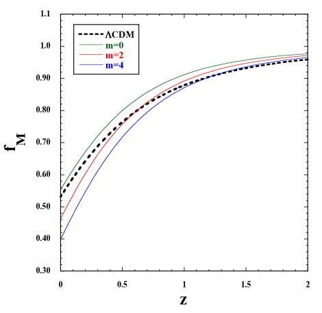
Figure 3: Evolution of $f_{M}=\dot{\delta}_{M}/(H\delta_{M})$ versus $z$ for the same background initial conditions of density parameters as those used in Fig. 1. The model parameters are $s=1/5$, $p_{2}=1$, and $r_{\beta}=0.05$ with three different values of $m$. The dotted line corresponds to the evolution of $f_{M}$ in the $\Lambda$CDM model.

In the right panel of Fig. 2, we plot the evolution of $\delta_{c}$, $\delta_{b}$, $\delta_{M}$, and $\Phi$ for the same model parameters and background initial conditions as those used in the left. Here, $\delta_{M}$ is the total density contrast defined by

$$\delta_{M}=\frac{\Omega_{c}}{\Omega_{c}+\Omega_{b}}\delta_{c}+\frac{\Omega_{b}}{\Omega_{c}+\Omega_{b}}\delta_{b}\,.$$ (199)

We numerically solve Eqs. (147) and (151) with Eqs. (148) and (152) derived under the quasi-static approximation for linear perturbations deep inside the sound horizon. We start to integrate the perturbation equations around the redshift $z=50$ by choosing the initial conditions $\delta_{c}=\delta_{c}^{\prime}=\delta_{i}$ and $\delta_{b}=\delta_{b}^{\prime}=\delta_{i}$. The initial amplitude $\delta_{i}$ is determined by reproducing today’s observed matter density contrast $\delta_{M}(z=0)$, where we adopt the Planck2018 best-fit value $\delta_{M}(z=0)=0.811$ Aghanim:2018eyx .

Since neither $G_{cc}$ nor $G_{bb}$ depends on the wavenumber $k$, the CDM and baryon perturbations exhibit scale-independent growth. In Fig. 2, we observe that the growth of $\delta_{c}$ is suppressed relative to that of $\delta_{b}$ for the redshift $z\lesssim 1$. This behavior is attributed to the gravitational interaction of CDM weaker than that of baryons. Since the CDM density is about five times as large as the baryon density, the total density contrast $\delta_{M}$ is mostly affected by CDM perturbations and hence its growth is suppressed in comparison to the standard case with $G_{cc}=G_{bb}=G$. This should allow the possibility for alleviating the tension of $\sigma_{8}$ between CDM and low-redshift measurements.

In our theory there is no anisotropic stress, so the gravitational potential $\Psi$ and the weak lensing potential $\psi_{\rm WL}=(\Psi-\Phi)/2$ are equivalent to each other, i.e., $\Psi=\psi_{\rm WL}=-\Phi$. In some models like cubic-order uncoupled scalar Galileons where both $G_{cc}$ and $G_{bb}$ are larger than $G$, $|\psi_{\rm WL}|$ grows even after the onset of cosmic acceleration Kobayashi:2009wr ; Kimura:2011td . This typically induces a negative ISW-galaxy cross-correlation, which is disfavored observationally Renk:2017rzu . In our coupled GP theory, $G_{cc}$ can be smaller than $G$ at low redshifts, so it is possible to avoid the enhancement of $|\psi_{\rm WL}|$. In the numerical simulation of Fig. 2, we observe that $\Phi~{}(=-\psi_{\rm WL})$ decreases at low redshifts.

In Fig. 3, we show the evolution of the matter growth rate $f_{M}=\dot{\delta}_{M}/(H\delta_{M})$ for three different values of $m$, with the other model parameters and initial conditions same as those used in Fig. 2. When $m=0$, we have $q_{c}=1$, $\epsilon_{c}=0$, and $c_{S}^{2}=\hat{c}_{S}^{2}$ in Eqs. (147) and (148), so the equation of CDM density contrast reduces to the same form as that of baryons with the gravitational coupling $G_{cc}=(1+\alpha_{\rm B}^{2}/\hat{\nu}_{S})G$. Since $G_{cc}=G_{bb}>G$ in this case, the growth rate $f_{M}$ is larger than that in the $\Lambda$CDM model, see Fig. 3. In contrast, for $m\beta>0$, the CDM gravitational coupling $G_{cc}$ can be smaller than $G$ at low redshifts. In the numerical simulation of Fig. 3, the growth rate $f_{M}$ for $m=2$ becomes smaller than that in the $\Lambda$CDM model at the redshift $z<0.62$. For increasing $m$, the suppression of $f_{M}$ tends to be more significant, see the case $m=4$ in Fig. 3. Thus, our coupled dark energy model with the momentum transfer offers a versatile possibility for realizing the weak cosmic growth rate. When our model is confronted with the observations of redshift-space distortions, however, we need to caution that the growth rates of $\delta_{c}$ and $\delta_{b}$ are different from each other. The analysis of how to constrain the model with the redshift-space distortion data is left for future work.

VI Conclusions

We studied the cosmology in coupled cubic-order GP theories given by the action (2) for the purpose of realizing the weak gravitational interaction on scales relevant to the growth of large-scale structures. The new interaction between the CDM four velocity $u_{c}^{\mu}$ and the vector field $A_{\mu}$, which is weighed by the scalar product $Z=-u_{c}^{\mu}A_{\mu}$, exhibits very different properties in comparison to the standard coupled dark energy with the energy transfer. The perfect fluids of CDM can be described by the Schutz-Sorkin action (3), which contains a vector density field $J_{c}^{\mu}$ related to the four velocity as $J_{c}^{\mu}=n_{c}\sqrt{-g}\,u_{c}^{\mu}$. After deriving general covariant equations of motion in the forms (17) and (20), we applied them to the flat FLRW background (23). As we observe in Eqs. (25) and (31), the $Z$ dependence in the coupling $f$ does not give rise to explicit interacting terms on the right-hand-sides of background continuity equations, by reflecting the fact that the interaction corresponds to the momentum transfer.

In Sec. III, we derived the second-order actions of tensor, vector, and scalar perturbations by choosing the flat gauge given by the line element (39). Tensor perturbations propagate in the same way as in the standard general relativity, so the theory is consistent with the observational bound of speed of gravity constrained by the GW170817 event. The new interaction does not affect small-scale stability conditions of vector perturbations either. For scalar perturbations, we obtained the full linear perturbation equations of motion and eliminated nondynamical variables from the second-order action. The resulting action for dynamical perturbations can be expressed in the form (93), which was exploited for the derivation of small-scale stability conditions. Under the conditions (101), (102), and (112) there are neither ghosts nor Laplacian instabilities, with the vanishing effective CDM sound speed.

In Sec. IV, we studied the effective gravitational couplings for CDM and baryon density perturbations by employing the quasi-static approximation for the modes deep inside the sound horizon. In our theory, there is no anisotropic stress between the two gravitational potentials $\Psi$ and $\Phi$, but the $Z$ dependence in $f$ induces the time derivative $\dot{\delta}_{c}$ to $\Phi$ and the longitudinal scalar $\psi$ of $A_{\mu}$, see Eqs. (145) and (146). Differentiating $\Phi$ and $\psi$ with respect to $t$ gives rise to the second derivative $\ddot{\delta}_{c}$ in Eq. (122) of the CDM density contrast. After closing the second-order differential equation of $\delta_{c}$, the gravitational coupling for CDM is given by the form (148). In contrast to the baryon gravitational coupling (152), there are extra terms proportional to $\alpha_{\rm B}$ in $G_{cc}$, besides the overall factor $\hat{c}_{S}^{2}/(q_{S}c_{S}^{2})$. The terms proportional to $\alpha_{\rm B}$, which correspond to the mixture of couplings $G_{3}(X)$ and $f(Z)$, lead to a value of $G_{cc}$ very different from $G_{bb}$ on the de Sitter background, see Eq. (154).

In Sec. V, we proposed a concrete coupled dark energy model given by the functions (161). For the powers (164), the background cosmology satisfying the relation $\phi^{p}H={\rm constant}$ ($p>0$) can be realized, with the new coupling constant $\beta$ being absorbed into the definition of $\Omega_{\rm DE}$. In other words, the interaction associated with the momentum transfer does not modify the cosmological background of uncoupled GP theories. We also showed that the ghosts are absent under the conditions (180) and (181). The scalar propagation speed squared in each cosmological epoch is given by Eqs. (185), (186), and (187), which are required to be all positive. The case shown in Fig. 1 is an example of the viable cosmology satisfying all the stability conditions.

During the matter dominance, the CDM gravitational coupling $G_{cc}$ is expanded in the form (191), which can be used to estimate the moment after which $G_{cc}$ gets smaller than $G$. Provided that the condition (195) is satisfied, the transition to the regime $G_{cc}<G$ occurs by today. On the future de Sitter attractor, $G_{cc}$ is given by Eq. (197), which is always negative in the allowed parameter space constrained by the no-ghost and no-strong-coupling conditions ($0<p_{2}\leq 1$). In the numerical simulation of Fig. 2, which corresponds to the power $p_{2}=1$, $G_{cc}$ enters the region $G_{cc}<G$ around $z<1$ and finally approaches the value $(G_{cc})_{\rm dS}=-u_{\rm dS}^{2}G=-0.225G$. In contrast, $G_{bb}$ is always larger than $G$. The weak gravitational interaction for CDM leads to the suppressed growth of total matter density contrast $\delta_{M}$, see Fig. 2. The lensing gravitational potential $\psi_{\rm WL}~{}(=-\Phi)$ does not exhibit the enhancement at low redshifts, whose property should be consistent with the observations of ISW-galaxy cross-correlations. For increasing values of $m$ and $\beta$, the growth rates of $\delta_{c}$ and $\delta_{M}$ tend to be smaller in comparison to the $\Lambda$CDM model, see Fig. 3.

We thus showed that the coupled GP theories with the momentum transfer offers a novel possibility for achieving the weak cosmic growth for CDM, in spite of the enhancement of baryon gravitational coupling. It will be of interest to investigate further whether the interacting model proposed in this paper reduces the observational tensions of $\sigma_{8}$ and $H_{0}$ present in the $\Lambda$CDM model.

References

- (1) P. J. E. Peebles, Astrophys. J. 284, 439 (1984).
- (2) P. J. E. Peebles, Astrophys. J. 263, L1 (1982).
- (3) A. G. Riess et al., Astrophys. J. 826, 56 (2016) [arXiv:1604.01424 [astro-ph.CO]].
- (4) N. Aghanim et al. [Planck Collaboration], arXiv:1807.06209 [astro-ph.CO].
- (5) L. Verde, T. Treu and A. G. Riess, Nature Astronomy, 3, 891-895 (2019) [arXiv:1907.10625 [astro-ph.CO]].
- (6) A. G. Riess, S. Casertano, W. Yuan, L. M. Macri and D. Scolnic, Astrophys. J. 876, no. 1, 85 (2019) [arXiv:1903.07603 [astro-ph.CO]].
- (7) W. L. Freedman et al., arXiv:1907.05922 [astro-ph.CO].
- (8) K. C. Wong et al., arXiv:1907.04869 [astro-ph.CO].
- (9) M. J. Reid, D. W. Pesce and A. G. Riess, Astrophys. J. 886, no. 2, L27 (2019) [arXiv:1908.05625 [astro-ph.GA]].
- (10) E. Macaulay, I. K. Wehus and H. K. Eriksen, Phys. Rev. Lett. 111, 161301 (2013) [arXiv:1303.6583 [astro-ph.CO]].
- (11) S. Nesseris, G. Pantazis and L. Perivolaropoulos, Phys. Rev. D 96, 023542 (2017) [arXiv:1703.10538 [astro-ph.CO]].
- (12) H. Hildebrandt et al., Mon. Not. Roy. Astron. Soc. 465, 1454 (2017) [arXiv:1606.05338 [astro-ph.CO]].
- (13) S. Joudaki et al., Mon. Not. Roy. Astron. Soc. 474, 4894 (2018) [arXiv:1707.06627 [astro-ph.CO]].
- (14) E. J. Copeland, M. Sami and S. Tsujikawa, Int. J. Mod. Phys. D 15, 1753 (2006) [hep-th/0603057].
- (15) Y. Fujii, Phys. Rev. D 26, 2580 (1982).
- (16) B. Ratra and P. J. E. Peebles, Phys. Rev. D 37, 3406 (1988).
- (17) C. Wetterich, Nucl. Phys. B 302, 668 (1988) [arXiv:1711.03844 [hep-th]].
- (18) P. G. Ferreira and M. Joyce, Phys. Rev. D 58, 023503 (1998) [astro-ph/9711102].
- (19) T. Chiba, N. Sugiyama and T. Nakamura, Mon. Not. Roy. Astron. Soc. 289, L5-L9 (1997) [arXiv:astro-ph/9704199 [astro-ph]].
- (20) T. Chiba, A. De Felice and S. Tsujikawa, Phys. Rev. D 87, 083505 (2013) [arXiv:1210.3859 [astro-ph.CO]].
- (21) S. Tsujikawa, Class. Quant. Grav. 30, 214003 (2013) [arXiv:1304.1961 [gr-qc]].
- (22) W. Hu and I. Sawicki, Phys. Rev. D 76, 064004 (2007) [arXiv:0705.1158 [astro-ph]].
- (23) S. Tsujikawa, K. Uddin, S. Mizuno, R. Tavakol and J. Yokoyama, Phys. Rev. D 77, 103009 (2008) [arXiv:0803.1106 [astro-ph]].
- (24) A. De Felice and S. Tsujikawa, Phys. Rev. Lett. 105, 111301 (2010) [arXiv:1007.2700 [astro-ph.CO]].
- (25) A. De Felice, L. Heisenberg, R. Kase, S. Mukohyama, S. Tsujikawa and Y. Zhang, JCAP 06, 048 (2016) [arXiv:1603.05806 [gr-qc]].
- (26) B. P. Abbott et al. [LIGO Scientific and Virgo Collaborations], Phys. Rev. Lett. 119, 161101 (2017) [arXiv:1710.05832 [gr-qc]].
- (27) A. Goldstein et al., Astrophys. J. 848, no. 2, L14 (2017) [arXiv:1710.05446 [astro-ph.HE]].
- (28) L. Lombriser and A. Taylor, JCAP 1603, 031 (2016) [arXiv:1509.08458 [astro-ph.CO]].
- (29) P. Creminelli and F. Vernizzi, Phys. Rev. Lett. 119, 251302 (2017) [arXiv:1710.05877 [astro-ph.CO]].
- (30) J. M. Ezquiaga and M. Zumalacarregui, Phys. Rev. Lett. 119, 251304 (2017) [arXiv:1710.05901 [astro-ph.CO]].
- (31) J. Sakstein and B. Jain, Phys. Rev. Lett. 119, 251303 (2017) [arXiv:1710.05893 [astro-ph.CO]].
- (32) T. Baker, E. Bellini, P. G. Ferreira, M. Lagos, J. Noller and I. Sawicki, Phys. Rev. Lett. 119, 251301 (2017) [arXiv:1710.06394 [astro-ph.CO]].
- (33) M. Crisostomi and K. Koyama, Phys. Rev. D 97, 084004 (2018) [arXiv:1712.06556 [astro-ph.CO]].
- (34) R. Kase and S. Tsujikawa, Phys. Rev. D 97, 103501 (2018) [arXiv:1802.02728 [gr-qc]].
- (35) L. Heisenberg, JCAP 1405, 015 (2014) [arXiv:1402.7026 [hep-th]].
- (36) G. Tasinato, JHEP 1404, 067 (2014) [arXiv:1402.6450 [hep-th]].
- (37) G. Tasinato, Class. Quant. Grav. 31, 225004 (2014) [arXiv:1404.4883 [hep-th]].
- (38) P. Fleury, J. P. B. Almeida, C. Pitrou and J. P. Uzan, JCAP 1411, 043 (2014). [arXiv:1406.6254 [hep-th]].
- (39) M. Hull, K. Koyama and G. Tasinato, Phys. Rev. D 93, 064012 (2016) [arXiv:1510.07029 [hep-th]].
- (40) E. Allys, P. Peter and Y. Rodriguez, JCAP 1602, 004 (2016) [arXiv:1511.03101 [hep-th]].
- (41) J. B. Jimenez and L. Heisenberg, Phys. Lett. B 757, 405 (2016) [arXiv:1602.03410 [hep-th]].
- (42) E. Allys, J. P. Beltran Almeida, P. Peter and Y. Rodriguez, JCAP 1609, 026 (2016) [arXiv:1605.08355 [hep-th]].
- (43) L. Amendola, M. Kunz, I. D. Saltas and I. Sawicki, Phys. Rev. Lett. 120, 131101 (2018) [arXiv:1711.04825 [astro-ph.CO]].
- (44) A. De Felice, L. Heisenberg, R. Kase, S. Mukohyama, S. Tsujikawa and Y. l. Zhang, Phys. Rev. D 94, 044024 (2016) [arXiv:1605.05066 [gr-qc]].
- (45) A. De Felice, L. Heisenberg and S. Tsujikawa, Phys. Rev. D 95, 123540 (2017) [arXiv:1703.09573 [astro-ph.CO]].
- (46) S. Nakamura, A. De Felice, R. Kase and S. Tsujikawa, Phys. Rev. D 99, 063533 (2019) [arXiv:1811.07541 [astro-ph.CO]].
- (47) A. De Felice, C. Q. Geng, M. C. Pookkillath and L. Yin, arXiv:2002.06782 [astro-ph.CO].
- (48) T. Kobayashi, H. Tashiro and D. Suzuki, Phys. Rev. D 81, 063513 (2010) [arXiv:0912.4641 [astro-ph.CO]].
- (49) R. Kimura, T. Kobayashi and K. Yamamoto, Phys. Rev. D 85, 123503 (2012) [arXiv:1110.3598 [astro-ph.CO]].
- (50) S. Nakamura, R. Kase and S. Tsujikawa, JCAP 1912, 032 (2019) [arXiv:1907.12216 [gr-qc]].
- (51) L. G. Gomez and Y. Rodriguez, arXiv:2004.06466 [gr-qc].
- (52) C. Wetterich, Astron. Astrophys. 301, 321 (1995) [hep-th/9408025].
- (53) L. Amendola, Phys. Rev. D 62, 043511 (2000) [astro-ph/9908023].
- (54) L. Amendola, Phys. Rev. D 69, 103524 (2004) [astro-ph/0311175].
- (55) A. Pourtsidou, C. Skordis and E. J. Copeland, Phys. Rev. D 88, 083505 (2013) [arXiv:1307.0458 [astro-ph.CO]].
- (56) C. G. Boehmer, N. Tamanini and M. Wright, Phys. Rev. D 91, 123003 (2015) [arXiv:1502.04030 [gr-qc]].
- (57) C. Skordis, A. Pourtsidou and E. J. Copeland, Phys. Rev. D 91, 083537 (2015) [arXiv:1502.07297 [astro-ph.CO]].
- (58) J. Dutta, W. Khyllep and N. Tamanini, Phys. Rev. D 95, 023515 (2017) [arXiv:1701.00744 [gr-qc]].
- (59) T. S. Koivisto, E. N. Saridakis and N. Tamanini, JCAP 1509, 047 (2015) [arXiv:1505.07556 [astro-ph.CO]].
- (60) A. Pourtsidou and T. Tram, Phys. Rev. D 94, 043518 (2016) [arXiv:1604.04222 [astro-ph.CO]].
- (61) R. Kase and S. Tsujikawa, Phys. Rev. D 101, 063511 (2020) [arXiv:1910.02699 [gr-qc]].
- (62) R. Kase and S. Tsujikawa, Phys. Lett. B 804, 135400 (2020) [arXiv:1911.02179 [gr-qc]].
- (63) F. N. Chamings, A. Avgoustidis, E. J. Copeland, A. M. Green and A. Pourtsidou, arXiv:1912.09858 [astro-ph.CO].
- (64) L. Amendola and S. Tsujikawa, arXiv:2003.02686 [gr-qc].
- (65) A. De Felice, L. Heisenberg, R. Kase, S. Tsujikawa, Y. Zhang and G. Zhao, Phys. Rev. D 93, 104016 (2016) [arXiv:1602.00371 [gr-qc]].
- (66) M. C. Pookkillath, A. De Felice and S. Mukohyama, Universe 6, no.1, 6 (2019).
- (67) B. F. Schutz and R. Sorkin, Annals Phys. 107, 1 (1977).
- (68) J. D. Brown, Class. Quant. Grav. 10, 1579 (1993) [gr-qc/9304026].
- (69) A. De Felice, J. M. Gerard and T. Suyama, Phys. Rev. D 81, 063527 (2010) [arXiv:0908.3439 [gr-qc]].
- (70) B. Boisseau, G. Esposito-Farese, D. Polarski and A. A. Starobinsky, Phys. Rev. Lett. 85, 2236 (2000) [gr-qc/0001066].
- (71) S. Tsujikawa, Phys. Rev. D 76, 023514 (2007) [arXiv:0705.1032 [astro-ph]].
- (72) A. De Felice, T. Kobayashi and S. Tsujikawa, Phys. Lett. B 706, 123 (2011) [arXiv:1108.4242 [gr-qc]].
- (73) A. De Felice and S. Tsujikawa, JCAP 02, 007 (2012) [arXiv:1110.3878 [gr-qc]].
- (74) A. De Felice and S. Tsujikawa, JCAP 03, 025 (2012) [arXiv:1112.1774 [astro-ph.CO]].
- (75) J. Renk, M. Zumalacarregui, F. Montanari and A. Barreira, JCAP 1710, 020 (2017) [arXiv:1707.02263 [astro-ph.CO]].