Spectral theory of fluctuations in time-average statistical mechanics of reversible and driven systems

Abstract

We present a spectral-theoretic approach to time-average statistical mechanics for general, non-equilibrium initial conditions. We consider the statistics of bounded, local additive functionals of reversible as well as irreversible ergodic stochastic dynamics with continuous or discrete state-space. We derive exact results for the mean, fluctuations and correlations of time average observables from the eigenspectrum of the underlying generator of Fokker-Planck or master equation dynamics, and discuss the results from a physical perspective. Feynman-Kac formulas are re-derived using Itô calculus and combined with non-Hermitian perturbation theory. The emergence of the universal central limit law in a spectral representation is shown explicitly on large deviation time-scales. For reversible dynamics with equilibrated initial conditions we derive a general upper bound to fluctuations of occupation measures in terms of an integral of the return probability. Simple, exactly solvable examples are analyzed to demonstrate how to apply the theory. As a biophysical example we revisit the Berg-Purcell problem on the precision of concentration measurements by a single receptor. Our results are directly applicable to a diverse range of phenomena underpinned by time-average observables and additive functionals in physical, chemical, biological, and economical systems.

I Introduction

Many experiments on soft and biological matter, such as single-particle tracking Saxton (2008); Metzler et al. (2014); Ernst et al. (2014); Shen et al. (2017) and single-molecule spectroscopy Hughes and Dougan (2016); Xie (1996); Ambrose et al. (1999); Plakhotnik et al. (1997); Neuman and Nagy (2008); Rief and Grubmüller (2002); Woodside and Block (2014); Ritort (2006); Camunas-Soler et al. (2016), probe individual trajectories. It is typically not feasible to repeat these experiments sufficiently many times in order to allow for ensemble-averaging. It is, however, straightforward to analyze such data by means of time-averaging along individual realizations. However, except for (ergodically) long observations, time-averages inferred from individual trajectories are random with non-trivial statistics. This naturally leads to the study of statistical properties of time-averages which formally represent functionals of stochastic processes.

The study of functionals of stochastic processes has a long tradition in mathematics (see e.g. Lévy (1940); Kac (1949); Darling and Kac (1957); Lamperti (1958); Feller (1949); Bingham (1975); Borodin (1989); Yen and Yor (2013)) and finance Yor (2001); Geman and Yor (1993). In physics they were found to be relevant in the context of diffusion-controlled chemical reactions (e.g. Wilemski and Fixman (1973); Szabo (1989); Bénichou et al. (2005)), transport in porous media Grebenkov (2007), chemical inference Berg and Purcell (1977); Wiegel (1983); Bialek and Setayeshgar (2005); Endres and Wingreen (2009); Mora and Wingreen (2010); Lang et al. (2014); Mora (2015); Barato and Seifert (2015); Aquino et al. (2015); Hartich and Seifert (2016), astrophysical observations Ferraro and Zaninetti (2004), medical diagnostics Gandjbakhche and Weiss (2000), optical imaging Weiss and Calabrese (1996), the study of growing surfaces Toroczkai et al. (1999), blinking of colloidal quantum dots Brokmann et al. (2003); Stefani et al. (2009), mesoscopic physics Comtet et al. (2005), climate Majumdar and Bray (2002) and computer science Majumdar, Satya N. (2005), and most recently in single-molecule spectroscopy Wennmalm et al. (1997); Gopich and Szabo (2012); Fleury et al. (2000); Barkai et al. (2004) and diffusion studies Agmon (2010), to name a few.

From a theoretical point of view analytical results were obtained for the occupation time statistics for discrete- state Markov switching Wennmalm et al. (1997); Gopich and Szabo (2012); Fleury et al. (2000); Barkai et al. (2004), for the local time at zero and occupation time above zero of a Brownian particle diffusing in a simple one-dimensional potential Majumdar, Satya N. (2005); Sabhapandit et al. (2006); Majumdar and Comtet (2002), the occupation time inside a spherical domain of a Brownian particle moving in free space Agmon (2010) and for a free, uniformly biased and harmonically bound particle undergoing subdiffusion Bel and Barkai (2005); Carmi and Barkai (2011). Exact results were also obtained for occupation time statistics for a general class of Markov processes Dhar and Majumdar (1999) and a discrete stationary non-Markovian sequence Majumdar and Dean (2002). Large deviation functions for various non-linear functionals of a class of Gaussian stationary Markov processes were studied in Majumdar and Bray (2002). Numerous important results on functionals have also been obtained in the context of persistence in spatially extended non-equilibrium systems Bray et al. (2013). Exact results were recently obtained on local times for projected observables in stochastic many-body systems Lapolla and Godec (2018, 2019), which provided insight into the emergence of memory on the level of individual non-Markovian trajectories. Notwithstanding, a general approach to fluctuations in time-average statistical mechanics for arbitrary initial conditions remains elusive.

Here, we present a spectral-theoretic approach to finite time-average statistical mechanics of ergodic systems. In mathematical terms we focus on the statistics of bounded, local, additive functionals of normal ergodic Markovian stochastic processes with continuous and discrete state-spaces, incl. functionals of their (non-Markovian) lower-dimensional projections. The paper is organized as follows. We first provide in Sec. II a brief introduction into time-average statistical mechanics. In Sec. III we re-derive the well-known Feynman-Kac formulas for Markovian diffusion using Itô calculus. In Sec. IV.1 spectral theory combined with non-Hermitian perturbation theory is applied to obtain our main result – exact expressions for the mean, variance and correlations of time-average observables for any non-stationary preparation of the system, expressed explicitly in terms of the eigenspectrum of the underlying generator of the dynamics, which may correspond to Fokker-Planck diffusion or Markovian dynamics governed by a master equation. We demonstrate explicitly the emergence of a central limit law in a spectral representation on large deviation time-scales. In Sec. IV.3 we derive our second main result – a general upper bound on fluctuations of occupation measures in terms of an integral of the, generally non-Markovian, return probability that is valid for generators of overdamped dynamics obeying detailed balance. Finally, simple analytically solvable examples are provided in Sec. V to demonstrate how to apply the theory. We conclude in Sec. VI.

II Time-average statistical mechanics

II.1 Ensemble- versus time-average observables

Traditional (classical) ensemble statistical mechanics describes physical observations as averages over individual realizations of the dynamics at single (or multiple) pre-determined times. For example, the ensemble average of an observable $V(\mathbf{x}_{t})$ at a time $t$ for an ergodic stochastic process $\mathbf{x}_{\tau}$ ($0\leq\tau\leq t$) starting from some non-stationary initial condition $p_{0}(\mathbf{x}_{0})$ is defined by

$$\langle V(\mathbf{x}_{t})\rangle_{p_{0}}\!\equiv\!\left\{\begin{array}[]{@{}ll@{}}\displaystyle\int_{\Omega}\!\!d\mathbf{x}\!\!\int_{\Omega}\!\!d\mathbf{x}_{0}V(\mathbf{x})P_{t}(\mathbf{x}|\mathbf{x}_{0})p_{0}(\mathbf{x}_{0})&\text{$\Omega\subset\mathbb{R}^{d}$,}\\ \displaystyle\sum_{\mathbf{x}\in\Omega}\sum_{\mathbf{x}_{0}\in\Omega}V(\mathbf{x})P_{t}(\mathbf{x}|\mathbf{x}_{0})p_{0}(\mathbf{x}_{0})&\text{$\Omega$ discrete,}\end{array}\right.$$ (1)

where $\Omega$ is the state space of the process and $P_{t}(\mathbf{x}|\mathbf{x}_{0})$ is the so-called propagator, i.e. $P_{t}(\mathbf{x}|\mathbf{x}_{0})d\mathbf{x}$ (upper line) is the probability that the process is found in $\mathbf{x}\in\Omega$ within the increment $d\mathbf{x}$ at time $t$ given that it started at $t=0$ at $\mathbf{x}_{0}$.

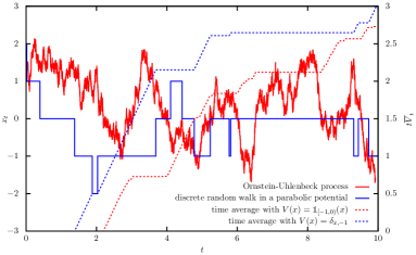
Figure 1: Realization of a trajectory $\mathbf{x}_{t}$ (solid lines) of a continuous Ornstein-Uhlenbeck diffusion (red) and a Markovian discrete-space continuous time random walk in a quadratic potential (blue). The dotted lines refer to the time average, Eq. (3), with $t\overline{V}_{t}=\int_{0}^{t}V(x_{\tau})d\tau$, where we chose $V(x)=\mathbbm{1}_{[0,1)}(x)$ for the Ornstein-Uhlenbeck and $V(x)=\delta_{-1,x}$ for the discrete random walk.

Note that if $\mathbf{x}$ is continuously valued ($\mathbf{x}\in\Omega\subset\mathbb{R}^{d}$; see Fig. 1 solid red line) then $P_{t}(\mathbf{x}|\mathbf{x}_{0})$ is a probability density, whereas if $\mathbf{x}$ is from a discrete state space $\Omega$ (Fig. 1 solid blue line) the integral in Eq. (1) (upper line) becomes a sum $\int_{\Omega}d\mathbf{x}\to\sum_{\mathbf{x}\in\Omega}$ and $P_{t}(\mathbf{x}|\mathbf{x}_{0})$ becomes a plain probability as shown in the lower line of Eq. (1). If $\mathbf{x}_{0}$ is sampled and averaged over a stationary (invariant) measure $p(\mathbf{x}_{0})=P_{\mathrm{inv}}(\mathbf{x}_{0})$ or $t$ becomes sufficiently (i.e. ergodically) large $P_{\infty}(\mathbf{x}|\mathbf{x}_{0})\equiv P_{\mathrm{inv}}(\mathbf{x})$ the ensemble average becomes time-independent

$$\langle V\rangle_{\mathrm{inv}}\equiv\int d\mathbf{x}V(\mathbf{x})P_{\mathrm{inv}}(\mathbf{x}).$$ (2)

Conversely, in single-molecule dynamics, single-particle tracking and other related experiments one probes individual realizations of $\mathbf{x}_{\tau}$ within the interval $0\leq\tau\leq t$ and instead analyzes the observation by taking a time-average. Such time-average observables are in general random, fluctuating quantities with non-trivial statistics. For example, for a physical observable $V(\mathbf{x}_{t})$, which may correspond to the squared displacement Boyer et al. (2012a, b) or local time Agmon (2010); Lapolla and Godec (2018, 2019); Jørgensen et al. (2005) in single particle tracking or the FRET efficiency Hughes and Dougan (2016); Xie (1996); Ambrose et al. (1999); Plakhotnik et al. (1997) or distance between two optical traps Neuman and Nagy (2008); Rief and Grubmüller (2002); Woodside and Block (2014); Ritort (2006); Camunas-Soler et al. (2016) in single-molecule fluorescence and force spectroscopy, respectively, the (local) time-average is defined as

$$\overline{V}_{t}\equiv t^{-1}\int_{0}^{t}V(\mathbf{x}_{\tau})d\tau$$ (3)

and depends on the entire history of $\mathbf{x}_{\tau}$ until time $t$ (see also dotted lines in Fig. 1). The statistical evolution of $\overline{V}_{t}$ is therefore a non-Markovian process characterized by the probability density that the random observable $\overline{V}_{t}$ attains, in a given realization of $\mathbf{x}_{\tau}$, the value $\nu$ Majumdar, Satya N. (2005); Sabhapandit et al. (2006); Majumdar and Comtet (2002); Lapolla and Godec (2018, 2019) which is defined as

$$\mathcal{P}^{\overline{V}}_{t}(\nu|\mathbf{x}_{0})\equiv\langle\delta(\nu-\overline{V}_{t})\rangle_{\mathbf{x}_{0}},$$ (4)

where $\delta(z)$ is the Dirac delta function and $\langle\cdot\rangle_{\mathbf{x}_{0}}$ denotes the average over all paths starting at $\mathbf{x}_{0}$, i.e. $p_{0}(\mathbf{x})=\delta(\mathbf{x}-\mathbf{x}_{0})$, and propagating until time $t$. The corresponding result for arbitrary initial conditions $p_{0}(\mathbf{x}_{0})$, follows by superposition, i.e. $\mathcal{P}^{\overline{V}}_{t}(\nu|p_{0})\equiv\int_{\Omega}\mathcal{P}^{\overline{V}}_{t}(\nu|\mathbf{x}_{0})p_{0}(\mathbf{x}_{0})d\mathbf{x}_{0}$ (see also Sec. III.2).

The random “empirical density” Barato and Chetrite (2015) $\theta_{\mathbf{x}}(t)$ determined from a single trajectory in time-average statistical mechanics is the so-called local time fraction defined as Yen and Yor (2013); Lapolla and Godec (2018, 2019)

$$\theta_{\mathbf{x}}(t)\equiv t^{-1}\int_{0}^{t}d\tau\delta(\mathbf{x}-\mathbf{x}_{\tau}),$$ (5)

which allows to rewrite the time average (3) in the form

$$\overline{V}_{t}=t^{-1}\!\!\int_{0}^{t}\!d\tau\!\!\int_{\Omega}\!d\mathbf{x}\delta(\mathbf{x}-\mathbf{x}_{\tau})V(\mathbf{x})\equiv\!\!\int_{\Omega}\!d\mathbf{x}V(\mathbf{x})\theta_{\mathbf{x}}(t),$$ (6)

where $\delta(\mathbf{x}-\mathbf{x}_{\tau})$ denotes the Dirac delta function if $\mathbf{x}\in\Omega$ is continuous, whereas $\delta(\mathbf{x}-\mathbf{x}_{\tau})$ denotes the Kronecker delta if $\mathbf{x}\in\Omega$ is integer-valued. Note that it is often useful to generalize the local time fraction in a point $\mathbf{x}$ in Eq. (5) to the notion of occupation time within the hypersurface $V(\mathbf{x})=\mathcal{V}$ defined as

$$\theta_{\mathcal{V}}(t)\equiv t^{-1}\int_{0}^{t}\delta(\mathcal{V}-V(\mathbf{x}_{\tau}))d\tau.$$ (7)

Accordingly, we can rewrite Eq. (6) equivalently in terms of $\theta_{\mathcal{V}}(t)$ as

$$\overline{V}_{t}=t^{-1}\!\!\int_{0}^{t}\!d\tau\!\!\int\!d\mathcal{V}\delta(\mathcal{V}-V(\mathbf{x}_{\tau}))\mathcal{V}\equiv\int d\mathcal{V}\mathcal{V}\theta_{\mathcal{V}}(t).$$ (8)

Because the dynamics $\mathbf{x}_{t}$ is assumed to be ergodic we have $\lim_{t\to\infty}\theta_{\mathbf{x}}(t)=P_{\mathrm{inv}}(\mathbf{x})$ and $\lim_{t\to\infty}\theta_{\mathcal{V}}(t)=P_{\mathrm{inv}}(\mathcal{V})$ Sabhapandit et al. (2006); Lapolla and Godec (2018, 2019) and

$$\lim_{t\to\infty} \overline{V}_{t}=\!\!\int\!\!d\mathbf{x}V(\mathbf{x})P_{\mathrm{inv}}(\mathbf{x})=\!\!\int\!\!d\mathcal{V}\mathcal{V}P_{\mathrm{inv}}(\mathcal{V})\equiv\langle V\rangle_{\mathrm{inv}},$$ (9)

$$\lim_{t\to\infty} \mathcal{P}^{\overline{V}}_{t}(\nu|\mathbf{x}_{0})=\delta(\nu-\langle V\rangle_{\mathrm{inv}}),$$

where we have defined the stationary (or invariant) measure of $\overline{V}(\mathbf{x}_{t})$, i.e. $P_{\mathrm{inv}}(\mathcal{V})\equiv\int d\mathbf{x}\delta(\mathcal{V}-V(\mathbf{x}_{\tau}))P_{\mathrm{inv}}(\mathbf{x})$.

Eqs. (9) reflect the strong law of large numbers on time-scales where $\overline{V}_{t}$ for different values of $t$ decorrelate. Moreover, on the so-called large-deviation time-scale, i.e. on the time-scale that is finite but longer that the longest relaxation time of $\mathbf{x}_{t}$, we find convergence in the mean, $\langle\overline{V}_{t_{\mathrm{LD}}}\rangle=\langle V\rangle_{\mathrm{inv}}$, and Gaussian fluctuations around the mean value Majumdar and Bray (2002); Touchette (2009, 2018); Lapolla and Godec (2018, 2019). For finite, and in particular sub-ergodic (i.e. supra-large deviation) times the statistics of $\overline{V}_{t}$ is, however, non-trivial. Below we provide intuition about the local time fraction from a practical perspective.

II.2 Local time fraction as a histogram inferred from a single trajectory

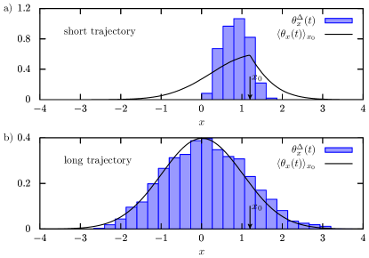
Figure 2: Local time fraction (or “empirical density”) for a Brownian particle in a harmonic potential. The histogram $\theta_{x}^{\Delta}(t)$ (blue) inferred from a single trajectory starting from $x_{0}=1.2$ compared the mean local time fraction $\langle\theta_{y}(t)\rangle_{x_{0}}=\lim_{\Delta\to 0}\langle\theta^{\Delta}_{y}(t)\rangle_{x_{0}}$. The histogram with bin-size $\Delta$ (here we assume $\Delta=0.3$) is defined by $\theta^{\Delta}_{x}(t)=\Delta^{-1}\int_{x-\Delta/2}^{x+\Delta/2}\theta_{y}(t)dy$, that is, $\theta_{x}^{\Delta}(t)=\overline{V}_{t}$ with $V(x)\equiv\Delta^{-1}\mathbbm{1}_{[x-\Delta/2,x+\Delta/2]}(x)$, where “$\mathbbm{1}$” denotes the indicator function being 1 if $x\in[x-\Delta/2,x+\Delta/2]$ and 0 otherwise. Parameters: $x_{0}=1.2$, (a) $t=1$; (b) $t=100$ (the trajectory is ten times as long as in Fig. 1).

To gain more intuition about the local time fraction (or “empirical density”) we consider, as an example, a Brownian particle diffusing in a harmonic potential. A single trajectory starting from $x_{0}=1.2$ is recorded as function of time (see full red line in Fig. 1). We are interested in the distribution (i.e. a histogram) of the particle’s position $x_{t}$ inferred from a single trajectory of length $t$ (see Fig. 2). Note that in Fig. 2 we consider a histogram with a finite bin-size $\Delta$, which we denote explicitly as $\theta_{x}^{\Delta}(t)$. In this sense the local time fraction (5) is simply a mathematical idealization of a histogram, i.e. $\theta_{x}(t)=\theta_{x}^{\Delta\to 0}(t)$.

In case the trajectory is sufficiently long (i.e. $t\to\infty$) $\theta_{x}^{\Delta}(t)$ converges, up to small fluctuations of order $1/\sqrt{t}$, to a Gaussian stationary (invariant) measure $P_{\mathrm{inv}}(x)\propto\mathrm{e}^{-x^{2}/2}$ (see Eq. (9)). This convergence is depicted explicitly in Fig. 2b. According to Eq. (9) this result depends neither on the initial condition $x_{0}$ nor on the particular realization of the trajectory.

We may also infer a histogram of the particle’s position from a short trajectory. The resulting histogram $\theta_{x}^{\Delta}(t)$ appears “rough” and far from Gaussian (see histogram in Fig. 2a). If we were to repeat the analysis for many trajectories and infer an averaged histogram $\langle\theta_{x}^{\Delta}(t)\rangle$ we would as well find that it deviates strongly from a Gaussian (see line in Fig. 2a) with large fluctuations around the mean, $\delta\theta_{x}^{\Delta}(t)\equiv|\theta_{x}^{\Delta}(t)-\langle\theta_{x}^{\Delta}(t)\rangle|\sim\langle\theta_{x}^{\Delta}(t)\rangle$ (see histogram in Fig. 2a) . Moreover, both the mean histogram $\langle\theta_{x}^{\Delta}(t)\rangle$ and the fluctuations around the mean, $\delta\theta_{x}^{\Delta}(t)$, depend not only of $t$ but also on the initial position $x_{0}$, where we observe a persistent cusp (Fig. 2a).

In the reminder of this work we will focus on the mean values and fluctuations of entries, as well as linear correlations between entries of such (random, realization-dependent) histograms inferred from finite, individual trajectories starting from general initial conditions.

II.3 Fluctuations of time averages

In order to exploit the role of the local time fraction $\theta_{\mathbf{x}}(t)$ as a “propagator” in time-average statistical mechanics (via $\overline{V}_{t}=\int_{\Omega}d\mathbf{x}V(\mathbf{x})\theta_{\mathbf{x}}(t)$) we now relate the statistics of $\theta_{\mathbf{x}}(t)$ to the probability density of a general time-averaged physical observable $\overline{V}_{t}$ defined in Eq. (3). In the example in Fig. 2 $\overline{V}_{t}=\theta^{\Delta}_{x}$ accounts for the value of the histogram at position $x$. The characteristic function of $\overline{V}_{t}$, i.e. the Laplace transform $\tilde{\mathcal{P}}^{\overline{V}}_{t}(u|\mathbf{x}_{0})\equiv\int_{0}^{\infty}\mathrm{e}^{-u\nu}\mathcal{P}^{\overline{V}}_{t}(\nu|\mathbf{x}_{0})d\nu$ if $\nu\geq 0$, reads

$$\tilde{\mathcal{P}}^{\overline{V}}_{t}(u|\mathbf{x}_{0})=\langle\mathrm{e}^{-u\overline{V}_{t}}\rangle_{\mathbf{x}_{0}}=\langle\mathrm{e}^{-u\int_{\Omega}V(\mathbf{x})\theta_{\mathbf{x}}(t)d\mathbf{x}}\rangle_{\mathbf{x}_{0}},$$ (10)

where we have used Eq. (6) to arrive at the second equality. Eq. (10) relates the statistics of the time average $\overline{V}_{t}$ to the statistics of all local time fractions $\theta_{\mathbf{x}}(t)$ ($\mathbf{x}\in\Omega$). We note that Eq. (10) must be modified if $V(\mathbf{x})$ can also become negative such that a Fourier transform is required instead, which amounts to replacing $u\to{\rm i}\omega$ with $\omega\in\mathbb{R}$ in Eq. (10). The probability density is obtained from Eq. (10) by Laplace inversion

$$\mathcal{P}^{\overline{V}}_{t}(\nu|\mathbf{x}_{0})=\frac{1}{2\pi{\rm i}}\int_{c-{\rm i}\infty}^{c+{\rm i}\infty}\mathrm{e}^{u\nu}\tilde{\mathcal{P}}^{\overline{V}}_{t}(u|\mathbf{x}_{0})du$$ (11)

where $c\in\mathbb{R}$ lies to the right of all singularities of $\tilde{\mathcal{P}}^{\overline{V}}_{t}(u|\mathbf{x}_{0})$ and we have assumed that $\mathcal{P}^{\overline{V}}_{t}(\nu|\mathbf{x}_{0})$ is of exponential order for sufficiently large $\nu$ (in the following section the conditions on $V(\mathbf{x}_{\tau})$ will be made more precise). In case the support extends to negative values of Eq. (11) becomes the inverse Fourier transform. Here we are particularly interested in fluctuations of time averages $\overline{V}_{t}$ and $\overline{W}_{t}$ of different physical observables $V(\mathbf{x}_{\tau})$ and $W(\mathbf{x}_{\tau})$ which are quantified by Lapolla and Godec (2018, 2019)

$$\sigma^{2}_{\overline{V}}(t) \equiv \langle\overline{V}_{t}^{2}\rangle_{\mathbf{x}_{0}}-\langle\overline{V}_{t}\rangle_{\mathbf{x}_{0}}^{2},$$

$$C_{\overline{V}\overline{W}}(t) \equiv \langle\overline{V}_{t}\overline{W}_{t}\rangle_{\mathbf{x}_{0}}-\langle\overline{V}_{t}\rangle_{\mathbf{x}_{0}}\langle\overline{W}_{t}\rangle_{\mathbf{x}_{0}},$$ (12)

where $\sigma^{2}_{V}(t)=C_{\overline{VV}}(t)$ denotes the variance of $\overline{V}_{t}$ and $C_{\overline{V}\overline{W}}(t)$ the covariance between $\overline{V}_{t}$ and $\overline{W}_{t}$.

In the example in Fig. 2, where $\overline{V}_{t}=\theta_{x}^{\Delta}(t)$ corresponds to the entry $x$ in the histogram, $\sigma^{2}_{\overline{V}}(t)\equiv\langle\delta\theta_{x}^{\Delta}(t)^{2}\rangle$ refers to the variance of said entries between different realizations of the histogram (i.e. the scatter of $\theta_{x}^{\Delta}(t)$ around $\langle\theta_{x}(t)\rangle$). Analogously, $C_{\overline{V}\overline{W}}(t)$ accounts for linear correlations between pairs of entries at $x$ and $y$, $\theta_{x}^{\Delta}(t)$ and $\theta_{y}^{\Delta}(t)$, in a histogram inferred from a single trajectory of length $t$.

Using Eq. (10) we obtain more generally

$$\langle\overline{V}_{t}^{n}\overline{W}_{t}^{m}\rangle_{\mathbf{x}_{0}}=\prod_{i=1}^{n}\int_{\Omega}d\mathbf{x}_{i}V(\mathbf{x}_{i})\prod_{j=1}^{m}\int_{\Omega}d\mathbf{y}_{j}W(\mathbf{y}_{j})\\ \times\langle\theta_{\mathbf{x}_{1}}(t)\cdots\theta_{\mathbf{x}_{n}}(t)\theta_{\mathbf{y}_{1}}(t)\cdots\theta_{\mathbf{y}_{m}}(t)\rangle_{\mathbf{x}_{0}},$$ (13)

where $\mathbf{x}_{i},\mathbf{y}_{j}\in\Omega$, respectively. Thereby, the ensemble average corresponding to the last term in Eq. (13) is obtained by differentiating the characteristic function with respect to the Laplace (or Fourier) variable.

It therefore follows, that the fluctuations and (linear) correlations of general time-average observables are fully specified by multi-point correlations functions of the local time fraction. These are derived on the basis of the Feynman-Kac formalism, which is presented below for continuous diffusion processes. The extension to discrete state dynamics is discussed afterwards.

III Fluctuations of additive functionals

III.1 Itô approach to Feynman-Kac theory of additive functionals

It seems to be customary in the physics literature to start from a path integral approach to Feynman-Kac theory Majumdar, Satya N. (2005) and in the following to derive a backward Fokker-Planck equation for the characteristic function Sabhapandit et al. (2006); Majumdar and Comtet (2002). Here we provide a simple derivation of the “forward” Feynman-Kac theory based on Itô calculus.

We consider a $d$-dimensional Markovian diffusion $\mathbf{x}_{t}\in\Omega\subset\mathbb{R}^{d}$ process in the presence of a drift $\mathbf{F}(\mathbf{x})$ driven by a $d$-dimensional Gaussian white noise governed by the Itô equation

$$d\mathbf{x}_{t}=\mathbf{F}(\mathbf{x}_{t})dt+\bm{\sigma}d\mathbf{W}_{t},$$ (14)

where $\bm{\sigma}$ is a $d\times d$ noise matrix such that $\mathbf{D}=\bm{\sigma}\bm{\sigma}^{T}/2$ becomes a symmetric positive (semi)definite diffusion matrix, $d\mathbf{W}_{t}$ is an increment of a $d$-dimensional Wiener process, such that $\langle{W}_{t}\rangle=\mathbf{0}$ and $\langle dW_{t,i}dW_{t^{\prime},j}\rangle=\delta(t-t^{\prime})\delta_{ij}dt$. We assume throughout that $\mathbf{F}(\mathbf{x})$ is sufficiently confining to assure that the process $\mathbf{x}_{t}$ is ergodic with a steady state probability density $P_{\mathrm{inv}}(\mathbf{x})$. Multiplying the time average in Eq. (3) by the trajectory length $t$ we transform the time average to the additive functional

$$\psi_{t}\equiv t\overline{V}_{t}=\int_{0}^{t}V(\mathbf{x}_{\tau})d\tau.$$ (15)

We now consider the joint process of $\mathbf{x}_{t}$ and $\psi_{t}$. According to Itô’s lemma any twice differentiable function $f(\mathbf{x},\psi)$ with $\mathbf{x}_{t}$ and $\psi_{t}$ defined by Eqs. (14) and (15), respectively, satisfies

$$df(\mathbf{x}_{t},\psi_{t})=[\mathbf{F}(\mathbf{x}_{t})\cdot\nabla_{\mathbf{x}}f(\mathbf{x}_{t},\psi_{t})+\nabla_{\mathbf{x}}\cdot\mathbf{D}\nabla_{\mathbf{x}}f(\mathbf{x}_{t},\psi_{t})]dt\\ +\nabla_{\mathbf{x}}f(\mathbf{x}_{t},\psi_{t})\cdot\bm{\sigma}d\mathbf{W}_{t}+V(\mathbf{x}_{t})\partial_{\psi}f(\mathbf{x}_{t},\psi_{t})dt,$$ (16)

where we inserted the diffusion matrix $\mathbf{D}=\bm{\sigma}\bm{\sigma}^{T}/2$ and for the last term we used $d\psi_{t}=V(\mathbf{x}_{t})dt$ that follows from Eq. (15).

Using Itô’s lemma (16) we derive in the following the time evolution of the joint probability density $Q_{t}(\mathbf{x},\psi|\mathbf{x}_{0})$ to find the system in state $\mathbf{x}$ and the functional $\psi_{t}$ in Eq. (15) to attain the value $\psi$ at time $t$ given that the system started from $\mathbf{x}_{0}$. For convenience we first focus on positive functionals ($\psi\geq 0$). Using a test function that vanishes at the boundary $f(\mathbf{x},0)=0$ we obtain after some calculations Gardiner (2004)

$$\frac{d}{dt}\langle f(x_{t},\psi_{t})\rangle_{\mathbf{x}_{0}} = \int_{0}^{\infty}d\psi\int_{\Omega}d\mathbf{x}f(\mathbf{x},\psi)\partial_{t}Q_{t}(\mathbf{x},\psi|\mathbf{x}_{0})$$ (17)

$$= \int_{0}^{\infty}d\psi\int_{\Omega}d\mathbf{x}Q_{t}(\mathbf{x},\psi|\mathbf{x}_{0})[\mathbf{F}(\mathbf{x})\cdot\nabla_{\mathbf{x}}f(\mathbf{x},\psi)+\nabla_{\mathbf{x}}\cdot\mathbf{D}\nabla_{\mathbf{x}}f(\mathbf{x},\psi)+V(\mathbf{x})\partial_{\psi}f(\mathbf{x},\psi)]$$

$$= \int_{0}^{\infty}d\psi\int_{\Omega}d\mathbf{x}f(\mathbf{x},\psi)[-\nabla_{\mathbf{x}}\cdot\mathbf{F}(\mathbf{x})+\nabla_{\mathbf{x}}\cdot\mathbf{D}\nabla_{\mathbf{x}}-V(\mathbf{x})\partial_{\psi}]Q_{t}(\mathbf{x},\psi|\mathbf{x}_{0})$$

which is obtained as follows. In the first line of Eq. (17) we differentiate both sides of the identity $\int_{0}^{\infty}d\mathbf{x}\int d\psi f(\mathbf{x},\psi)Q_{t}(\mathbf{x},\psi|\mathbf{x}_{0})=\langle f(\mathbf{x}_{t},\psi_{t})\rangle_{\mathbf{x}_{0}}$ with respect to time $t$. To obtain the second line we inserted Itô’s Lemma (16) and finally performed an integration by parts. Since Eq. (17) holds for any function $f$ that vanishes at the boundary $\psi=0$ we obtain

$$\partial_{t}Q_{t}(\mathbf{x},\psi|\mathbf{x}_{0})=\left[\hat{L}-V(\mathbf{x})\partial_{\psi}-V(\mathbf{x})\delta(\psi)\right]Q_{t}(\mathbf{x},\psi|\mathbf{x}_{0}),$$ (18)

where we have defined the forward generator $\hat{L}=\nabla_{\mathbf{x}}\cdot\mathbf{D}\nabla_{\mathbf{x}}-\nabla_{\mathbf{x}}\cdot\mathbf{F}(\mathbf{x})$ and further introduced a boundary term $V(\mathbf{x})\delta(\psi)Q_{t}(\mathbf{x},0|\mathbf{x}_{0})$ that vanishes for $\psi>0$ and is derived in the following two steps. First, Eq. (17) holds for all functions $f(\mathbf{x},\psi)$ with $f(\mathbf{x},0)=0$, which immediately gives Eq. (18) without the last term for $\psi>0$ (see also Gardiner (2004)). Second, the last term in Eq. (18) is required to guarantee the conservation of probability $\int_{0}^{\infty}d\psi\int_{\Omega}d\mathbf{x}\partial_{t}Q_{t}(\mathbf{x},\psi|\mathbf{x}_{0})=0$, i.e., to correct for the fact that there is a non-zero probability that the functional has a vanishing value $\psi=0$. Finally, performing a Laplace transform of Eq. (18), $\tilde{Q}_{t}(\mathbf{x},u|\mathbf{x}_{0})\equiv\int_{0}^{\infty}\mathrm{e}^{-u\psi}Q_{t}(\mathbf{x},\psi|\mathbf{x}_{0})d\psi=blue\langle\delta(\mathbf{x}-\mathbf{x}_{t})\mathrm{e}^{-u\psi_{t}}\rangle_{\mathbf{x}_{0}}$, we obtain the forward Feynman-Kac partial differential equation for the characteristic function of the joint density of position and $\psi$

$$\partial_{t}\tilde{Q}_{t}(\mathbf{x},u|\mathbf{x}_{0})=(\hat{L}-uV(\mathbf{x}))\tilde{Q}_{t}(\mathbf{x},u|\mathbf{x}_{0}),$$ (19)

where $Q_{t}(\mathbf{x},\psi|\mathbf{x}_{0})$ is the central object of the ’forward’ Feynman-Kac approach Kac (1949); Majumdar, Satya N. (2005).

We now relax the assumption by allowing for a negative support of $\psi_{t}$, which we denote explicitly by $\psi_{t}\to\Psi_{t}$. In this case we need not to make any additional assumptions on $f(\mathbf{x}_{t},\Psi_{t})$ for $\Psi_{t}=0$ because naturally $\lim_{|\Psi|\to\infty}Q_{t}(\mathbf{x},\Psi|\mathbf{x}_{0})=0$. The lower boundary of integration over $\Psi$ in Eq. (17) is extended to $-\infty$ and the boundary terms resulting from the partial integration vanish as a result of the boundary conditions. The resulting Eq. (17) implies

$$\partial_{t}Q_{t}(\mathbf{x},\Psi|\mathbf{x}_{0})=\left(\hat{L}-V(\mathbf{x})\partial_{\Psi}\right)Q_{t}(\mathbf{x},\Psi|\mathbf{x}_{0}),$$ (20)

which upon taking a Fourier transform $\tilde{Q}_{t}(\mathbf{x},\omega|\mathbf{x}_{0})\equiv\int_{-\infty}^{\infty}\mathrm{e}^{-{\rm i}\omega\Psi}Q_{t}(\mathbf{x},\Psi|\mathbf{x}_{0})d\Psi$ leads to the forward Feynman-Kac partial differential equation

$$\partial_{t}\tilde{Q}_{t}(\mathbf{x},\omega|\mathbf{x}_{0})=(\hat{L}-{\rm i}\omega V(\mathbf{x}))\tilde{Q}_{t}(\mathbf{x},\omega|\mathbf{x}_{0}),$$ (21)

Note that the generalization to the case of a joint problem for multiple functionals $\psi^{i}_{t}$ with $i=1,\ldots,p$ is straightforward. Introducing the vectorial notation $\bm{\psi}_{t}\equiv\int_{0}^{t}\mathbf{V}(\mathbf{x}_{\tau})d\tau$ with the corresponding Laplace images $\mathbf{u}$ the resulting equation reads

$$\partial_{t}\tilde{Q}_{t}(\mathbf{x},\mathbf{u}|\mathbf{x}_{0})=(\hat{L}-\mathbf{u}\cdot\mathbf{V}(\mathbf{x}))\tilde{Q}_{t}(\mathbf{x},\mathbf{u}|\mathbf{x}_{0}),$$ (22)

which allows for the computation of higher-order correlation functions (13). What we actually seek for is the marginal probability density of $\bm{\psi}$ given $\mathbf{x}_{0}$ defined by

$$\mathcal{P}^{\bm{\psi}}_{t}(\bm{\psi}|\mathbf{x}_{0})\equiv\int_{\Omega}Q_{t}(\mathbf{x},\bm{\psi}|\mathbf{x}_{0})d\mathbf{x},$$ (23)

which is the statement of the Feynman-Kac theorem Kac (1949). Note that the corresponding characteristic function $\tilde{\mathcal{P}}^{\bm{\psi}}_{t}(\mathbf{u}|\mathbf{x}_{0})=\int_{\Omega}\mathrm{e}^{-\mathbf{u}\cdot\bm{\psi}}\mathcal{P}^{\bm{\psi}}_{t}(\bm{\psi}|\mathbf{x}_{0})d\bm{\psi}\equiv\langle\mathrm{e}^{-\mathbf{u}\cdot\bm{\psi}_{t}}\rangle_{\mathbf{x}_{0}}$ is the solution of the ’backward’ Feynman-Kac problem Sabhapandit et al. (2006); Majumdar and Comtet (2002). Moreover, the marginal probability density of $\mathbf{x}$ given $\mathbf{x}_{0}$ corresponds to the plain propagator $P_{t}(\mathbf{x}|\mathbf{x}_{0})\equiv\int Q_{t}(\mathbf{x},\bm{\psi}|\mathbf{x}_{0})d\bm{\psi}$, which solves the (forward) Fokker-Planck equation $(\partial_{t}-\hat{L})P_{t}(\mathbf{x}|\mathbf{x}_{0})=0$ with initial data $P_{0}(\mathbf{x}|\mathbf{x}_{0})=\delta(\mathbf{x}-\mathbf{x}_{0})$.

Note that the characteristic functions $\tilde{\mathcal{P}}^{\overline{\mathbf{V}}}_{t}$ and $\tilde{\mathcal{P}}^{\bm{\psi}}_{t}$ are equivalent up to a trivial rescaling of the independent variable, i.e.

$$\tilde{\mathcal{P}}^{\overline{\mathbf{V}}}_{t}(\mathbf{u}|\mathbf{x}_{0})=\langle\mathrm{e}^{-\mathbf{u}\cdot\overline{\mathbf{V}}_{t}}\rangle=\langle\mathrm{e}^{-\mathbf{u}/t\cdot\bm{\psi}_{t}}\rangle=\tilde{\mathcal{P}}^{\bm{\psi}}_{t}(\mathbf{u}/t|\mathbf{x}_{0}).$$ (24)

Therefore, once $\tilde{\mathcal{P}}^{\bm{\psi}}_{t}$ is determined according to the Feynman-Kac program a simple change of scale of the Laplace image $\mathbf{u}\to\mathbf{u}/t$ delivers $\tilde{\mathcal{P}}^{\overline{\mathbf{V}}}_{t}$.

III.2 From the forward to the backward Feynman-Kac equation

For convenience we henceforth adopt the bra-ket notation, where the “ket” $|h\rangle$ denotes a vector, the “bra” the integral operator $\langle g|\equiv\int_{\Omega}d\mathbf{x}g^{\dagger}(\mathbf{x})$, and the scalar product is defined as $\langle g|h\rangle\equiv\int_{\Omega}d\mathbf{x}g^{\dagger}(\mathbf{x})h(\mathbf{x})$. Introducing, moreover, the “flat” state $|-\rangle\equiv\int_{\Omega}d\mathbf{x}|\mathbf{x}\rangle$ and $\langle-|\equiv\int_{\Omega}d\mathbf{x}\langle\mathbf{x}|$, Eqs. (21) and (22) for a general initial condition $p_{0}(\mathbf{x})$, i.e. $|p_{0}\rangle=\int_{\Omega}d\mathbf{x}_{0}p_{0}(\mathbf{x}_{0})|\mathbf{x}_{0}\rangle$ and $\langle p_{0}|=\int_{\Omega}d\mathbf{x}_{0}p_{0}(\mathbf{x}_{0})\langle\mathbf{x}_{0}|$, have the solution Lapolla and Godec (2018)

$$\tilde{\mathcal{P}}^{\bm{\psi}}_{t}(\mathbf{u}|p_{0})\equiv\langle-|\mathrm{e}^{t(\hat{L}-\mathbf{u}\cdot\mathbf{V}(\mathbf{x}))}|p_{0}\rangle=\langle p_{0}|\mathrm{e}^{t(\hat{L}^{\dagger}-\mathbf{u}\cdot\mathbf{V}(\mathbf{x}))}|-\rangle.$$ (25)

To arrive at the second equality we have used Green’s identity, introduced the adjoint (or backward) Fokker-Planck operator $\hat{L}^{\dagger}=\nabla_{\mathbf{x}}\cdot\mathbf{D}\nabla_{\mathbf{x}}+\mathbf{F}(\mathbf{x})\cdot\nabla_{\mathbf{x}}$, and used that the Laplace transform of a real function $f(t)$ transforms as $\tilde{f}(s^{\dagger})=\tilde{f}^{\dagger}(s)$ under complex conjugation. In the following subsection we show that for Markov jump processes (25) the theory can be adopted one-by-one.

III.3 Markov-jump dynamics and additive functionals

Markov jump processes correspond to a discrete state-space $\Omega$ in which the system jumps with a constant rate $w_{\mathbf{x}\mathbf{y}}$ from state $\mathbf{x}\in\Omega$ to another state $\mathbf{y}\in\Omega$, such that the propagator $P_{t}(\mathbf{x}|\mathbf{x}_{0})$ satisfies the master equation

$$\partial_{t}P_{t}(\mathbf{x}|\mathbf{x}_{0})=\sum_{\mathbf{y}}\langle\mathbf{x}|\hat{L}|\mathbf{y}\rangle P_{t}(\mathbf{y}|\mathbf{x}_{0}),$$ (26)

where $\langle\mathbf{x}|\hat{L}|\mathbf{y}\rangle=w_{\mathbf{y}\mathbf{x}}$ if $\mathbf{x}\neq\mathbf{y}$ and $\langle\mathbf{x}|\hat{L}|\mathbf{x}\rangle=-\sum_{\mathbf{y}\neq\mathbf{x}}\langle\mathbf{y}|\hat{L}|\mathbf{x}\rangle$ such that $-\langle\mathbf{x}|\hat{L}|\mathbf{x}\rangle>0$ is the rate of leaving state $\mathbf{x}$. According to the celebrated Gillespie algorithm Gillespie (1977) a single trajectory $\mathbf{x}_{\tau}$ ($0\leq\tau\leq t$) consist of a sequence exponentially distributed local waiting times $\tau_{i}$ in state $\mathbf{x}_{i}\in\Omega$ followed by an instantaneous transition to another state $\mathbf{x}_{i+1}\neq\mathbf{x}_{i}$, with the total time being the sum of waiting times $\sum_{i}\tau_{i}=t-\tau_{R}$, where $\tau_{R}$ is the duration of the final epoch that contains no jump. More precisely, whenever the system is in a state $\mathbf{x}_{i}$ at time $t_{i}$ the probability density to leave said state $\mathbf{x}_{i}$ exactly at time $t_{i+1}=t_{i}+\tau_{i}$ is exponentially distributed with a waiting time density $-\langle\mathbf{x}_{i}|\hat{L}|\mathbf{x}_{i}\rangle{\rm e}^{\langle\mathbf{x}_{i}|\hat{L}|\mathbf{x}_{i}\rangle\tau_{i}}$. After the waiting time a new (accessible) state, $\mathbf{x}_{i+1}$, is randomly chosen with probability $-\langle\mathbf{x}_{i+1}|\hat{L}|\mathbf{x}_{i}\rangle/\langle\mathbf{x}_{i}|\hat{L}|\mathbf{x}_{i}\rangle$. Therefore, the joint probability density that the system, starting from state $\mathbf{x}_{i}$, jumps after time $\tau_{i}$ and the following state is $\mathbf{x}_{i+1}$ becomes $\langle\mathbf{x}_{i+1}|\hat{L}|\mathbf{x}_{i}\rangle{\rm e}^{\langle\mathbf{x}_{i}|\hat{L}|\mathbf{x}_{i}\rangle\tau_{i}}$.

Denoting the number of transitions from state $\mathbf{x}$ to state $\mathbf{y}$ until a time $t$ by $n_{\mathbf{x}\mathbf{y}}(t)=\sum_{i}\delta_{\mathbf{x}_{i},\mathbf{x}}\delta_{\mathbf{x}_{i+1},\mathbf{y}}$ and identifying the sum of all local waiting times in state $\mathbf{x}$ up to time $t$ by $t\theta_{\mathbf{x}}(t)=\sum_{i}\delta_{\mathbf{x}_{i},\mathbf{x}}\tau_{i}$ the path probability (or path weight) of $\mathbf{x}_{\tau}$ ($0\leq\tau\leq t$) starting from $\mathbf{x}_{0}$ generated by the Markov dynamics (26) can be written as Hartich and Seifert (2016)

$$P(\{\mathbf{x}_{\tau}\}|\mathbf{x}_{0})=\prod_{\mathbf{x}\neq\mathbf{y}}[\langle\mathbf{x}|\hat{L}|\mathbf{y}\rangle]^{n_{\mathbf{y}\mathbf{x}}(t)}\mathrm{e}^{\sum_{\mathbf{x}}t\theta_{\mathbf{x}}(t)\langle\mathbf{x}|\hat{L}|\mathbf{x}\rangle}.$$ (27)

Replacing the integral in Eq. (6) by a sum, $\overline{V}_{t}=\sum_{\mathbf{x}}V(\mathbf{x})\theta_{\mathbf{x}}(t)$, allows us to identify the characteristic function of $\psi_{t}=t\overline{V}_{t}$ by Hartich and Seifert (2016)

$$\tilde{\mathcal{P}}^{\psi}_{t}(u|\mathbf{x}_{0}) \equiv\langle\mathrm{e}^{-ut\overline{V}_{t}}\rangle_{\mathbf{x}_{0}}$$

$$=\!\int\!d\{\mathbf{x}_{\tau}\}P(\{\mathbf{x}_{\tau}\}|\mathbf{x}_{0})\mathrm{e}^{-u\sum_{\mathbf{x}}V(\mathbf{x})t\theta_{\mathbf{x}}(t)}$$

$$=\langle-|\mathrm{e}^{\hat{L}(u)t}|\mathbf{x}_{0}\rangle$$ (28)

where in the second line we inserted the path weight Eq. (27). While passing from the second to the third line we tilted the diagonal of the generator in the path weight (27) according to $\langle\mathbf{x}|\hat{L}(u)|\mathbf{x}\rangle\equiv\langle\mathbf{x}|\hat{L}|\mathbf{x}\rangle-uV(\mathbf{x})$, which effectively moves $\mathrm{e}^{-ut\overline{V}_{t}}$ into the tilted path weight. In other words, identifying $\hat{L}(u)$ in the second line of Eq. (28) yields the third line. Note that the off-diagonal elements of the tilted generator remain unchanged, that is, $\langle\mathbf{x}|\hat{L}(u)|\mathbf{y}\rangle\equiv\langle\mathbf{x}|\hat{L}|\mathbf{y}\rangle$ if $\mathbf{x}\neq\mathbf{y}$. Since all elements of $\hat{L}$ and $V(\mathbf{x})$ are real, Eq. (25) holds also for Markov-jump processes. As shown in Eq. (24) the characteristic function of $\overline{V}_{t}=\psi_{t}/t$ follows from a trivial change of scale, $\tilde{\mathcal{P}}^{\overline{V}}_{t}(u|\mathbf{x}_{0})=\tilde{\mathcal{P}}^{\psi}_{t}(u/t|\mathbf{x}_{0})$. In the following we develop a spectral theory, which unifies diffusion processes and Markov-jump processes.

III.4 Spectral theory of non-Hermitian generators

We henceforth employ a spectral-theoretic approach and are thus required to make some more specific assumptions about the underlying dynamics in order to assure that the generator $\hat{L}$ is diagonalizable. An excellent account of the theory for Markov-jump dynamics governed by a discrete-state master equation can be found in Schnakenberg (1976). In the case of Fokker-Planck dynamics we consider that $\mathbf{x}_{t}$ is an ergodic Markovian diffusion evolving according to Eq. (14) with the drift field $\mathbf{F}(\mathbf{x})$ not necessarily corresponding to a potential field (which thus include systems with a broken detailed balance) but at the same time requiring that it is sufficiently confining, that is, it grows sufficiently fast as $|\mathbf{x}|\to\infty$ to assure that $\hat{L}$ has a pure point-spectrum. Moreover, we require that $\hat{L}$ is diagonalizable and it can be shown that any normal operator $\hat{L}$, satisfying $\hat{L}\hat{L}^{\dagger}=\hat{L}^{\dagger}\hat{L}$, is in fact diagonalizable Conway (1985). A more detailed mathematical exposé of the requirements for, and properties of, $\hat{L}$ can be found in Lapolla and Godec (2019). In all practical examples presented below we will in fact assume that the dynamics is overdamped. Moreover, except for the example presented in Sec. V.3 where detailed balance is violated, $\hat{L}$ will be assumed to obey detailed balance Gardiner (2004); van Kampen (2007), implying that it is orthogonally equivalent to a self-adjoint operator and hence automatically diagonalizable.

Let $-\lambda_{k}$ ($\mathrm{Re}(\lambda_{k})\geq 0$), $\langle L_{k}|$, and $|R_{k}\rangle$ denote the eigenvalue and orthonormal left and right eigenstates of $\hat{L}$, and $-\lambda_{k}^{\dagger}$, $\langle R_{k}|$ and $|L_{k}\rangle$ the corresponding orthonormal eigenstates of $\hat{L}^{\dagger}$ Lapolla and Godec (2019), i.e. $\langle L_{k}|R_{l}\rangle=\langle R_{k}|L_{l}\rangle=\delta_{kl}$, with the resolution of identity $\sum_{k}|R_{k}\rangle\langle L_{k}|\equiv\sum_{k}|L_{k}\rangle\langle R_{k}|=\mathbf{1}$. Then written in the respective eigenbases $\hat{L}$ and $\hat{L}^{\dagger}$ read

$$\hat{L}=-\sum_{k}\lambda_{k}|R_{k}\rangle\langle L_{k}|,\quad\hat{L}^{\dagger}=-\sum_{k}\lambda_{k}^{\dagger}|L_{k}\rangle\langle R_{k}|,$$ (29)

with the ground-state eigenvalue $\lambda_{0}=0$ and corresponding null-space $|R_{0}\rangle\equiv|P_{\mathrm{inv}}\rangle$ and $\langle L_{0}|\equiv\langle-|$. In the respective dual eigenbasis the propagator $P_{t}(\mathbf{x}|\mathbf{x}_{0})\equiv\langle\mathbf{x}|\mathrm{e}^{\hat{L}t}|\mathbf{x}_{0}\rangle=\langle\mathbf{x}_{0}|\mathrm{e}^{\hat{L}^{\dagger}t}|\mathbf{x}\rangle$ reads

$$P_{t}(\mathbf{x}|\mathbf{x}_{0}) = \sum_{k}\langle\mathbf{x}|R_{k}\rangle\langle L_{k}|\mathbf{x}_{0}\rangle\mathrm{e}^{-\lambda_{k}t}$$ (30)

$$\equiv \sum_{k}\langle\mathbf{x}_{0}|L_{k}\rangle\langle R_{k}|\mathbf{x}\rangle\mathrm{e}^{-\lambda^{\dagger}_{k}t},$$

where $\langle\mathbf{x}|R_{k}\rangle\equiv R_{k}(\mathbf{x})$ and $\langle L_{k}|\mathbf{x}_{0}\equiv L^{\dagger}_{k}(\mathbf{x}_{0})$, while $\langle\mathbf{x}_{0}|L_{k}\rangle=L_{k}(\mathbf{x}_{0})$ and $\langle R_{k}|\mathbf{x}\rangle=R^{\dagger}_{k}(\mathbf{x})$. For overdamped systems with invertible diffusion matrix $\mathbf{D}$ that obey detailed balance, i.e. $\mathbf{D}^{-1}\mathbf{F}(\mathbf{x})=-\beta\nabla_{\mathbf{x}}U(\mathbf{x})$ with inverse thermal energy $\beta=1/k_{\mathrm{B}}T$, all $\lambda_{k}$ are real, $|P_{\mathrm{inv}}\rangle=|P_{\mathrm{eq}}\rangle$ is the Boltzmann-Gibbs equilibrium $P_{\mathrm{eq}}(\mathbf{x})=\mathrm{e}^{-\beta U(\mathbf{x})}/\int_{\Omega}\mathrm{e}^{-\beta U(\mathbf{x})}d\mathbf{x}$, and $|L_{k}\rangle=\mathrm{e}^{\beta U(\mathbf{x})}|R_{k}\rangle$ Risken (1996); Gardiner (2004).

IV Characteristic function near zero via non-Hermitian perturbation theory

Based on Eqs. (10) and (13) we only require the moment-generating function (25), in the limit $|\mathbf{u}|\to 0$ to calculate moments of arbitrary order. Moreover, recall that $\tilde{\mathcal{P}}^{\overline{\mathbf{V}}}_{t}(\mathbf{u})=\tilde{\mathcal{P}}^{\bm{\psi}}_{t}(\mathbf{u}/t)$ (see Eq. (24)). To keep the treatment general we utilize the spectral expansion of $\hat{L}$ ($\hat{L}^{\dagger}$, respectively). We employ perturbation theory to derive the moment-generating function (25) in the limit $|\mathbf{u}|\to 0$. There are (at least) two possible ways to arrive at the result: a Dyson series approach, which is presented in Appendix B, and by means of second order non-Hermitian perturbation theory, which is detailed below. While both yield equivalent results, the perturbation-theoretic approach is more general as it provides a (bi)spectral expansion of the of the perturbed generator $\hat{L}-\mathbf{u}\cdot\mathbf{V}(\mathbf{x})$ ($\hat{L}^{\dagger}-\mathbf{u}\cdot\mathbf{V}(\mathbf{x})$, respectively) to second order in $|\mathbf{u}|$. These perturbation-theoretic results, which in the Physics literature appear to be new, are applicable beyond time-average statistical mechanics in diverse problems involving perturbations of non-Hermitian and/or non-self-adjoint eigenvalue problems.

Our aim is to diagonalize the “tilted” propagator in Eq. (25) in the limit when $\mathbf{u}$ vanishes. Because $\hat{L}$ is in general not self-adjoint we need to separately perturb left and right eigenstates. First we must confirm that the tilted propagator $\hat{L}(\mathbf{u})\equiv\hat{L}-\mathbf{u}\cdot\mathbf{V}(\mathbf{x})$ (and $\hat{L}^{\dagger}(\mathbf{u})\equiv\hat{L}^{\dagger}-\mathbf{u}\cdot\mathbf{V}(\mathbf{x})$, respectively) is actually diagonalizable in an arbitrarily small neighborhood of $\mathbf{u}=\mathbf{0}$. We focus first on the case where $V(\mathbf{x})\geq 0$. We Laplace transform Eq. (25) $t\to s$ yielding

$$\tilde{\mathcal{P}}^{\bm{\psi}}_{s}(\mathbf{u}|p_{0})\equiv\langle-|[s-\hat{L}(\mathbf{u})]^{-1}|p_{0}\rangle=\langle p_{0}|[s-\hat{L}^{\dagger}(\mathbf{u})]^{-1}|-\rangle.$$ (31)

The singularities of Eq. (31) correspond to the perturbed eigenvalue spectrum $\{-\lambda_{k}(\mathbf{u})\}$ of $\hat{L}(\mathbf{u}))$ and diagonalizability is broken whenever one or more singularities are not simple poles (see e.g. Stoller et al. (1991)). Eq. (25) shows that $|\mathbf{u}|=0$ is not an accumulation point. Moreover, $\hat{L}$ has a pure point spectrum therefore an arbitrarily small $|\mathbf{u}|$ cannot cause the emergence of poles of second order in Eq. (31) that would break diagonalizability, akin to the “avoided crossing theorem”. Therefore, in the limit $|\mathbf{u}|\to 0$ the tilted generator $\hat{L}(\mathbf{u})$ is diagonalizable, $\mathbf{u}$ can be taken as real , and the eigenspectrum of $\hat{L}(\mathbf{u})$ corresponds to a regular perturbation of the original eigenvalue problem $\hat{L}|R_{k}\rangle=-\lambda_{k}|R_{k}\rangle$ ($\hat{L}^{\dagger}|L_{k}\rangle=-\lambda_{k}^{\dagger}|L_{k}\rangle$) and we seek for a perturbative expansion of the tilted eigenspectrum, e.g. of $\hat{L}^{\dagger}(\mathbf{u})$:

$$-\lambda^{{}^{\prime}\dagger^{\prime}}_{k}(\mathbf{u}) = -\lambda^{\dagger}_{k}-\sum_{i>0}\mathbf{u}^{i}\cdot\bm{\lambda_{k}^{(i)}},$$

$$|L_{k}(\mathbf{u})\rangle = |L_{k}\rangle+\sum_{i>0}\mathbf{u}^{i}\cdot\mathbf{|L_{k}^{i}\rangle},$$

$$\langle R_{k}(\mathbf{u})| = \langle R_{k}|+\sum_{i>0}\mathbf{u}^{i}\cdot\mathbf{|R_{k}^{i}\rangle}.$$ (32)

Without loss of generality we will henceforth assume that $\mathbf{u}$ is real. Note that while the spectra of $\hat{L}$ and $\hat{L}^{\dagger}$ are complex conjugates (see Eq. (29)) the perturbation is in fact symmetric (see Eq. (31)). Therefore, the spectra of $\hat{L}(u)$ and $\hat{L}^{\dagger}(u)$ are not complex conjugates except for the unperturbed part, which we denoted in Eq. (32) by quotation marks $\lambda^{{}^{\prime}\dagger^{\prime}}$. According to Eq. (32) multiple functionals yield additive perturbations. It thus suffices to carry out the calculations for $\mathbf{u}\to u$ and write the corresponding general result by inspection. We are interested in up to second order moments (13) and therefore need to evaluate the perturbation up to second order in $u$:

$$\!\!\!\!\!(-\hat{L}^{\dagger}+uV)\sum_{n=0}^{2}u^{n}|L_{k}^{n}\rangle = \sum_{n=0}^{2}u^{n}\lambda_{k}^{(n)}\sum_{m=0}^{2}u^{m}|L_{k}^{m}\rangle,$$ (33)

$$\!\!\!\!\!\sum_{n=0}^{2}u^{n}\langle R_{k}^{n}|(-\hat{L}^{\dagger}+uV) = \sum_{n=0}^{2}u^{n}\lambda_{k}^{(n)}\sum_{m=0}^{2}u^{m}\langle R_{k}^{m}|,$$ (34)

where we have adopted the convention $\lambda_{k}^{(0)}\equiv\lambda^{\dagger}_{k}$, $\langle R_{k}^{0}|\equiv\langle R_{k}|$, and $|L_{k}^{0}\rangle\equiv|L_{k}\rangle$. In Eqs. (34) we only need to keep terms up to $u^{2}$ and equate terms of matching order in $u$. First we impose the preliminary normalization $\langle R_{k}(u)|L_{k}\rangle=\langle R_{k}|L_{k}(u)\rangle=1$, i.e.

$$1 = \langle R_{k}|L_{k}\rangle+u\langle R_{k}^{1}|L_{k}\rangle+u^{2}\langle R_{k}^{2}|L_{k}\rangle+\mathcal{O}(u^{3})$$

$$1 = \langle R_{k}|L_{k}\rangle+u\langle R_{k}|L_{k}^{1}\rangle+u^{2}\langle R_{k}|L_{k}^{2}\rangle+\mathcal{O}(u^{3}),$$ (35)

which implies

$$\langle R_{k}^{n}|L_{k}\rangle=\langle R_{k}|L_{k}^{n}\rangle=0,\quad\mathrm{for}\quad n>0.$$ (36)

The $0$-th order of the expansion gives the solution of the unperturbed system. For the higher orders we need to solve Eqs. (34) matching terms of equal order. Introducing the coupling elements $V_{lk}\equiv\langle R_{l}|V|L_{k}\rangle$ we obtain (details of the calculation are shown in Appendix A)

$$\lambda_{k}^{(1)} = V_{kk},\quad\lambda_{k}^{(2)}=\sum_{l\neq k}\frac{V_{kl}V_{lk}}{\lambda^{\dagger}_{k}-\lambda^{\dagger}_{l}},$$ (37)

$$|L_{k}^{1}\rangle = \sum_{l\neq k}\frac{V_{lk}}{\lambda^{\dagger}_{k}-\lambda^{\dagger}_{l}}|L_{l}\rangle,\quad\langle R_{k}^{1}|=\sum_{l\neq k}\frac{V_{kl}}{\lambda^{\dagger}_{k}-\lambda^{\dagger}_{l}}\langle R_{l}|,$$

$$|L_{k}^{2}\rangle = \sum_{l\neq k}\left[\sum_{i\neq k}\frac{V_{ik}V_{li}}{(\lambda^{\dagger}_{k}-\lambda^{\dagger}_{i})(\lambda^{\dagger}_{k}-\lambda^{\dagger}_{l})}-\frac{V_{kk}V_{lk}}{(\lambda^{\dagger}_{k}-\lambda^{\dagger}_{l})^{2}}\right]|L_{l}\rangle,$$

$$\langle R_{k}^{2}| = \sum_{l\neq k}\left[\sum_{i\neq k}\frac{V_{ki}V_{il}}{(\lambda^{\dagger}_{k}-\lambda^{\dagger}_{i})(\lambda^{\dagger}_{k}-\lambda^{\dagger}_{l})}-\frac{V_{kk}V_{kl}}{(\lambda^{\dagger}_{k}-\lambda^{\dagger}_{l})^{2}}\right]\langle R_{l}|.$$

However, while they are orthogonal by construction, the resulting perturbed eigenstates are not normalized anymore, i.e. $\langle R_{k}(u)|L_{k}(u)\rangle\neq 1$. Hence, we need to post-normalize them such that

$$\mathcal{N}_{k}(u)\langle R_{k}(u)|L_{k}(u)\rangle=1,$$ (38)

where from it follows that

$$\mathcal{N}_{k}(u) = \left[(\langle R_{k}|+\sum_{i=1}^{2}u^{i}\langle R_{k}^{i}|)(|L_{k}\rangle+\sum_{i=1}^{2}u^{i}|L_{k}^{i}\rangle)\right]^{-1}$$ (39)

$$= \frac{1}{1+u^{2}\langle R_{k}^{1}|L_{k}^{1}\rangle+\mathcal{O}(u^{3})}$$

$$= 1-u^{2}\sum_{i\neq k}\frac{V_{ki}V_{ik}}{(\lambda^{\dagger}_{k}-\lambda^{\dagger}_{i})^{2}}+\mathcal{O}(u^{3})$$

$$\equiv 1-u^{2}\mathcal{M}_{k}+\mathcal{O}(u^{3}),$$

where in the last line we have defined $\mathcal{M}_{k}$. We now use the second-order perturbed eigenspectrum to diagonalize the moment-generating function in Eq. (25)

$$\tilde{\mathcal{P}}^{\psi}_{t}(u|p_{0})=\sum_{k}\mathcal{N}_{k}(u)\langle p_{0}|L_{k}(u)\rangle\langle R_{k}(u)|-\rangle\mathrm{e}^{-\lambda^{{}^{\prime}\dagger^{\prime}}_{k}(u)t},$$ (40)

where moreover

$$\mathrm{e}^{-\lambda^{\dagger}_{k}(u)t}=\mathrm{e}^{-\lambda_{k}^{\dagger}t}[1-u\lambda_{k}^{(1)}t+u^{2}(\lambda_{k}^{(1)2}t^{2}/2-\lambda_{k}^{(2)}t)]+\mathcal{O}(u^{3})$$ (41)

and $\langle R_{k}(u)|-\rangle=\langle R_{k}|-\rangle+u\langle R_{k}^{1}|-\rangle+u^{2}\langle R_{k}^{2}|-\rangle+\mathcal{O}(u^{3})$ with the coefficients given by

$$\langle R_{k}|-\rangle = \delta_{k0},\quad\langle R_{k}^{1}|-\rangle=\frac{V_{k0}}{\lambda^{\dagger}_{k}}(1-\delta_{k0}),$$

$$\langle R_{k}^{2}|-\rangle = -\frac{V_{kk}V_{k0}}{\lambda_{k}^{\dagger 2}}+\sum_{i\neq k}\frac{V_{ki}V_{i0}}{\lambda^{\dagger}_{k}(\lambda^{\dagger}_{k}-\lambda^{\dagger}_{i})}(1-\delta_{k0})$$ (42)

and $\langle p_{0}|L_{k}(u)\rangle=\langle p_{0}|L_{k}\rangle+u\langle p_{0}|L_{k}^{1}\rangle+u^{2}\langle p_{0}|L_{k}^{2}\rangle+\mathcal{O}(u^{3})$, where $|L_{k}^{1}\rangle$ and $|L_{k}^{2}\rangle$ are given by Eq. (IV). Using Eqs. (IV), (39) as well as (41) and (42) the tilted propagator in Eq. (40) to second order in $u$ reads

$$\tilde{\mathcal{P}}^{\psi}_{t}(u|p_{0})=1+\sum_{k>0}\left(uC^{(1)}_{k}+u^{2}C^{(2)}_{k}\right)\mathrm{e}^{-\lambda_{k}^{\dagger}t}+\mathcal{O}(u^{3})$$ (43)

where we have introduced the coefficients

$$C^{(1)}_{k} = \delta_{k0}\left(-V_{00}t+\langle p_{0}|L^{1}_{0}\rangle\right)+\langle p_{0}|L_{k}\rangle\langle R^{1}_{k}|-\rangle$$

$$C^{(2)}_{k} = \delta_{k0}\left[\langle p_{0}|L_{0}\rangle\left(\mathcal{M}_{0}+V_{00}^{2}t^{2}/2-\lambda_{0}^{(2)}t\right)+\langle p_{0}|L^{2}_{0}\rangle\right]$$ (44)

$$- t\left(\langle p_{0}|L^{1}_{0}\rangle V_{00}\delta_{k0}-\langle p_{0}|L_{k}\rangle\langle R^{1}_{k}|-\rangle V_{kk}\right)$$

$$+ \langle p_{0}|L^{1}_{k}\rangle\langle R^{1}_{k}|-\rangle+\langle p_{0}|L_{k}\rangle\langle R^{2}_{k}|-\rangle$$

with $\mathcal{M}_{0}$ defined in the Eq. (39). In the special case when initial conditions $\mathbf{x}_{0}$ are drawn from the steady state probability density, i.e. $p_{0}(\mathbf{x})=P_{\mathrm{inv}}(\mathbf{x})$, these equations simplify to

$$\!\!\!\!\!\!\langle P_{\mathrm{inv}}|L_{k}\rangle = \delta_{k0},\quad\langle P_{\mathrm{inv}}|L_{k}^{1}\rangle=\frac{V_{0k}}{\lambda^{\dagger}_{k}}(1-\delta_{k0}),$$

$$\!\!\!\!\!\!\langle P_{\mathrm{inv}}|L_{k}^{2}\rangle = -\frac{V_{kk}V_{0k}}{\lambda_{k}^{\dagger 2}}+\sum_{i\neq k}\frac{V_{ik}V_{0i}}{\lambda^{\dagger}_{k}(\lambda^{\dagger}_{k}-\lambda^{\dagger}_{i})}(1-\delta_{k0}).$$ (45)

Turning now to the case where $V(\mathbf{x})$ extends negative values we must simply replace $u$ by $i\omega$. In order to obtain moments up to second order (i.e. Eq. (12) we are now left with evaluating derivatives of Eq. (43) with respect to $u$ at $u=0$.

IV.1 Mean value, fluctuations and correlation functions for general initial conditions

We can now derive the mean, variance and covariance of time-average observables. We first focus on the case of a single time-average observable $\overline{V}_{t}=\psi_{t}/t$ (see Eqs. (3) and (15)). According to Eq. (24) we must make the replacement $u\to u/t$ in Eq. (43). We will only present the result in terms of the spectrum of the backward generator $\hat{L}^{\dagger}$ since the results corresponding to $\hat{L}$ follow trivially from Eq. (25). Note that $\langle p_{0}|-\rangle=1$ for any normalized initial condition.

To order $u^{0}$ Eq. (43) simply reflects the normalization of $\mathcal{P}^{\overline{V}}_{t}(\nu|p_{0})$, i.e. $\tilde{\mathcal{P}}^{\overline{V}}_{t}(0|p_{0})=\int_{0}^{\infty}\mathcal{P}^{\overline{V}}_{t}(\nu|p_{0})d\nu=1$ (and equivalently in the case where the support of $\overline{V}_{t}$ extends to the entire real axis). To order $u^{1}$ Eq. (43) encodes the mean value $\langle\overline{V}_{t}\rangle_{p_{0}}$ since it follows from Eq. (10) that $-\partial_{u}\tilde{\mathcal{P}}^{\overline{V}}_{t}(u|p_{0})|_{u=0}=\int_{0}^{\infty}\nu\mathcal{P}^{\overline{V}}_{t}(\nu|p_{0})d\nu\equiv\langle\overline{V}_{t}\rangle_{p_{0}}$. Thus the mean value of a time-average observable $\langle\overline{V}_{t}\rangle_{p_{0}}$ evolving from an arbitrary initial condition $p_{0}(\mathbf{x})$ is given by

$$\langle\overline{V}_{t}\rangle_{p_{0}}=V_{00}+\frac{1}{t}\sum_{k>0}\frac{V_{k0}}{\lambda^{\dagger}_{k}}\langle p_{0}|L_{k}\rangle\left(1-\mathrm{e}^{-\lambda^{\dagger}_{k}t}\right),$$ (46)

with the anticipated ergodic limit $V_{00}=\langle\overline{V}_{t\to\infty}\rangle_{p_{0}}=\langle P_{\mathrm{inv}}|V|-\rangle\equiv\int_{\Omega}V(\mathbf{x})P_{\mathrm{inv}}(\mathbf{x})d\mathbf{x}$. The result (46) is equally valid in cases where $V(\mathbf{x})$ can become negative (as long as its is bounded). Moreover, from Eq. (46) is easy to discern the large deviation asymptotic

$$\lim_{t\gg 1/\mathrm{Re}\lambda^{\dagger}_{1}}\langle\overline{V}_{t}\rangle_{p_{0}}\simeq V_{00}+\frac{1}{t}\sum_{k>0}\frac{V_{k0}}{\lambda^{\dagger}_{k}}\langle p_{0}|L_{k}\rangle,$$ (47)

and in the special case of steady-state initial conditions $p_{0}(\mathbf{x}_{0})=P_{\mathrm{inv}}(\mathbf{x}_{0})$ Eq. (46) reduces to the time-independent ergodic result $\langle\overline{V}_{t}\rangle_{\mathrm{inv}}=V_{00}$. To order $u^{2}$ Eq. (43) encodes the second moment via $\partial^{2}_{u}\tilde{\mathcal{P}}^{\overline{V}}_{t}(u|p_{0})|_{u=0}=\int_{0}^{\infty}\nu^{2}\mathcal{P}^{\overline{V}}_{t}(\nu|\mathbf{x}_{0})d\nu\equiv\langle\overline{V}_{t}^{2}\rangle_{p_{0}}$, which reads

$$\langle\overline{V}_{t}^{2}\rangle_{p_{0}}=V_{00}^{2}+\frac{2}{t}\sum_{k>0}\frac{V_{k0}}{\lambda^{\dagger}_{k}}[V_{0k}+\langle p_{0}|L_{k}\rangle(V_{00}+V_{kk}\mathrm{e}^{-\lambda^{\dagger}_{k}t})]\\ +\frac{2}{t^{2}}\sum_{k>0}V_{k0}\bigg{\{}[\langle p_{0}|L_{k}\rangle(V_{kk}-V_{00})-V_{k0}]\frac{(1-\mathrm{e}^{-\lambda^{\dagger}_{k}t})}{\lambda_{k}^{\dagger 2}}\\ +\sum_{l>0,l\neq k}\frac{V_{lk}\langle p_{0}|L_{l}\rangle}{\lambda^{\dagger}_{k}-\lambda^{\dagger}_{l}}\left(\frac{1-\mathrm{e}^{-\lambda^{\dagger}_{l}t}}{\lambda^{\dagger}_{l}}-\frac{1-\mathrm{e}^{-\lambda^{\dagger}_{k}t}}{\lambda^{\dagger}_{k}}\right)\bigg{\}}$$ (48)

which together with Eq. (46) yields the variance

$$\sigma^{2}_{\overline{V},p_{0}}(t)\equiv\langle\overline{V}_{t}^{2}\rangle_{p_{0}}-\langle\overline{V}_{t}\rangle_{p_{0}}^{2}.$$ (49)

We further introduce the following notational convention for localized initial conditions $p_{0}(\mathbf{x})=\delta(\mathbf{x}-\mathbf{x}_{0})$, $\sigma^{2}_{\overline{V},p_{0}}(t)\to\sigma^{2}_{\overline{V},\mathbf{x}_{0}}(t)$. From Eqs.  (46), (48), and (49) follows the anticipated ergodic result $\langle\overline{V}^{2}_{t\to\infty}\rangle_{p_{0}}=V_{00}^{2}$, proving that in the ergodic limit $\overline{V}_{t}$ becomes deterministic (i.e. the variance vanishes, $\sigma^{2}_{\overline{V},p_{0}}(t\to\infty)=\langle\overline{V}^{2}_{t\to\infty}\rangle_{p_{0}}-\langle\overline{V}_{t\to\infty}\rangle_{p_{0}}^{2}=0$). Conversely the large-deviation asymptotic reads for any initial condition $p_{0}(\mathbf{x})$

$$\lim_{\mathrm{Re}\lambda^{\dagger}_{1}t\gg 1}\langle\overline{V}_{t}^{2}\rangle_{p_{0}}=V_{00}^{2}+\frac{2}{t}\sum_{k>0}\frac{V_{k0}}{\lambda^{\dagger}_{k}}\left(V_{0k}+V_{00}\langle p_{0}|L_{k}\rangle\right)$$ (50)

yielding a large-deviation variance

$$\!\lim_{\mathrm{Re}\lambda_{1}t\gg 1}\sigma^{2}_{\overline{V}}(t)=\frac{2}{t}\sum_{k>0}\frac{V_{0k}V_{k0}}{\lambda^{\dagger}_{k}}+\mathcal{O}(t^{-2}),$$ (51)

which embodies the emergence of the central limit theorem. One can further show that all higher cumulants decay to zero faster that $1/t$. Since the only distribution with a finite number of non-zero cumulants is the Gaussian distribution Marcinkiewicz (1939), the large deviation mean value (47) and variance (51) specify the entire asymptotic probability density for time-average observables along trajectories of length $t\gg 1/\mathrm{Re}\lambda^{\dagger}_{1}$.

In the special case of steady-state initial conditions, $p_{0}(\mathbf{x})=P_{\mathrm{inv}}(\mathbf{x})$, we find the variance satisfies (see also Lapolla and Godec (2018))

$$\sigma^{2}_{\overline{V},\mathrm{inv}}(t)=\frac{2}{t}\sum_{k>0}\frac{V_{0k}V_{k0}}{\lambda^{\dagger}_{k}}\left(1-\frac{1-\mathrm{e}^{-\lambda^{\dagger}_{k}t}}{\lambda^{\dagger}_{k}t}\right).$$ (52)

Note that for overdamped systems in detailed balance we have $\lambda^{\dagger}_{k}\in\mathbb{R}$ and $|L_{k}\rangle=\mathrm{e}^{\beta U(\mathbf{x})}|R_{k}\rangle\in\mathbb{R}$. Therefore $V_{0k}V_{k0}\geq 0$,which implies (compare Eqs. (51) and (52)) that the fluctuations for stationary initial conditions are bounded from above by $\sigma^{2}_{\overline{V},\mathrm{inv}}(t)\leq\lim_{\lambda^{\dagger}_{1}t\gg 1}\langle\overline{V}_{t}^{2}\rangle_{p_{0}}-V_{00}^{2}$ irrespective of $p_{0}(\mathbf{x})$.

We now inspect the correlation between two functionals $\overline{V}_{1,t}$ and $\overline{V}_{2,t}$ (see Eq. (12)) defined as $C_{\overline{V}_{1}\overline{V}_{2}}(t)=\langle\overline{V}_{1,t}\overline{V}_{2,t}\rangle_{p_{0}}-\langle\overline{V}_{1,t}\rangle_{p_{0}}\langle\overline{V}_{2,t}\rangle_{p_{0}}$. The mean values were derived in Eq. (46) so we only require the mixed second moment $\langle\overline{V}_{1,t}\overline{V}_{2,t}\rangle_{p_{0}}$, which is obtained from the joint moment-generating function (i.e. generalization of Eq. (40) to two variables) as $\langle\overline{V}_{1,t}\overline{V}_{2,t}\rangle_{p_{0}}=\partial^{2}_{u_{1}u_{2}}\tilde{\mathcal{P}}^{\overline{\mathbf{V}}}_{t}(\mathbf{u}|p_{0})|_{\mathbf{u}=\mathbf{0}}$. A lengthy calculation leads, upon introducing the coupling elements $U^{i}_{kl}\equiv\langle R_{k}|V_{i}(\mathbf{x})|L_{l}\rangle$ and the shorthand notation $W_{klmn}=U^{1}_{kl}U^{2}_{mn}+U^{2}_{kl}U^{1}_{mn}$, to the exact result

$$\langle\overline{V}_{1,t}\overline{V}_{2,t}\rangle_{p_{0}}=\frac{W_{0000}}{2}\\ +\frac{1}{t}\sum_{k>0}\frac{1}{\lambda_{k}^{\dagger}}\left(W_{k00k}+\langle p_{0}|L_{k}\rangle\left[W_{00k0}-W_{k0kk}\mathrm{e}^{-\lambda^{\dagger}_{k}t}\right]\right)\\ +\frac{1}{t^{2}}\sum_{k>0}\bigg{\{}[\langle p_{0}|L_{k}\rangle(W_{k0kk}-W_{00k0})-W_{k00k}]\frac{(1-\mathrm{e}^{-\lambda^{\dagger}_{k}t})}{\lambda_{k}^{\dagger 2}}\\ +\sum_{l>0,l\neq k}\frac{W_{k0lk}\langle p_{0}|L_{l}\rangle}{\lambda^{\dagger}_{k}-\lambda^{\dagger}_{l}}\left(\frac{1-\mathrm{e}^{-\lambda^{\dagger}_{l}t}}{\lambda^{\dagger}_{l}}-\frac{1-\mathrm{e}^{-\lambda^{\dagger}_{k}t}}{\lambda^{\dagger}_{k}}\right)\bigg{\}},$$ (53)

and we note that $\langle\overline{V}_{1,t}\rangle_{\mathrm{inv}}\langle\overline{V}_{2,t}\rangle_{\mathrm{inv}}=W_{0000}/2$ implying that for an ergodic system any two functionals asymptotically decorrelate, $\lim_{t\to\infty}C_{\overline{V}_{1}\overline{V}_{2}}(t)=0$. Equations (46), (48), and (53) expressing the mean value and second moments (and together the variance and covariance) of the time average of a general physical observable $V(\mathbf{x}_{\tau})$ of type Eq. (3) solely in terms of the eigenspectrum of the underlying generator are the main theoretical result of this work.

In the case of stationary initial conditions $p_{0}(\mathbf{x})=P_{\mathrm{inv}}(\mathbf{x})$ we have that $\langle P_{\mathrm{inv}}|L_{k}\rangle=\delta_{k0}$ and as a result of Eq. (53) the covariance reduces to (note that $W_{k00k}=W_{0kk0}$ and $W_{0000}/2=\langle\overline{V}_{1,t}\rangle_{\mathrm{inv}}\langle\overline{V}_{2,t}\rangle_{\mathrm{inv}}$)

$$C_{\overline{V}_{1}\overline{V}_{2}}^{\mathrm{inv}}(t)=\frac{1}{t}\sum_{k>0}\frac{W_{0kk0}}{\lambda^{\dagger}_{k}}\left(1-\frac{1-\mathrm{e}^{-\lambda^{\dagger}_{k}t}}{\lambda^{\dagger}_{k}t}\right).$$ (54)

Finally, in the large deviation regime we recover

$$\lim_{t\gg 1/\lambda_{1}}C_{\overline{V}_{1}\overline{V}_{2}}(t)=\frac{1}{t}\sum_{k>0}\frac{W_{0kk0}}{\lambda^{\dagger}_{k}}+\mathcal{O}(t^{-2})$$ (55)

the $1/t$ scaling reflecting the emergence of the central limit theorem. Therefore, it follows that an arbitrary set of $m$ time-average observables $\mathbf{\overline{V}}_{t}=\{\overline{V}_{i,t}\}$ in the large deviation limit exhibits Gaussian statistics. If we denote the vector of mean values as $\langle\mathbf{\overline{V}}\rangle_{\mathrm{inv}}$ and introduce the symmetric covariance matrix $\mathbf{C}$ with diagonal elements $\mathbf{C}_{ii}=t\lim_{t\gg 1/\mathrm{Re}\lambda_{1}}\sigma^{2}_{\overline{V}_{i}}(t)$ (see Es. (51)) and off-diagonal elements $\mathbf{C}_{ij}=t\lim_{t\gg 1/\mathrm{Re}\lambda_{1}}C_{\overline{V}_{i}\overline{V}_{j}}(t)$ (see Es. (55)) then the probability density that $\mathbf{\overline{V}}_{t}$ attains a value $\bm{\nu}$ obeys the asymptotic Gaussian limit law $\lim_{t\gg 1/\mathrm{Re}\lambda_{1}}\mathcal{P}^{\mathbf{\overline{V}}}_{t}(\bm{\nu}|p_{0})\equiv\mathcal{P}_{t}^{\mathrm{LD}}(\bm{\nu})$ where

$$\mathcal{P}_{t}^{\mathrm{LD}}(\bm{\nu})\simeq\frac{\displaystyle{\mathrm{e}^{-\frac{1}{2}(\bm{\nu}-\langle\mathbf{\overline{V}}\rangle_{\mathrm{inv}})^{T}\mathbf{C}^{-1}(\bm{\nu}-\langle\mathbf{\overline{V}}\rangle_{\mathrm{inv}})t}}}{\sqrt{(2\pi)^{m}\mathrm{det}\mathbf{C}/t}}.$$ (56)

We now introduce the rescaled variables $\hat{\bm{\nu}}\equiv\bm{\nu}\sqrt{t}$ and scaled mean $\bm{\mu}\equiv\langle\mathbf{\overline{V}}_{t}\sqrt{t}\rangle_{\mathrm{inv}}$, which upon re-normalization lead to a time-independent density. Moreover, we define

$$\Xi=(\hat{\nu}_{i}-\mu_{i})/\sqrt{\mathbf{C}_{ii}},\quad\Xi_{i|j}=(\hat{\nu}_{i}-\tilde{\mu}_{i|j})/\tilde{\sigma}_{i|j}$$ (57)

with the shifted mean and stretched variance

$$\tilde{\mu}_{i|j} = \mu_{i}+(\hat{\nu}_{j}-\mu_{j})\mathbf{C}_{ij}/\mathbf{C}_{jj}$$

$$\tilde{\sigma}^{2}_{i|j} = (\mathbf{C}_{ii}\mathbf{C}_{jj}-\mathbf{C}_{ij}^{2})/\mathbf{C}_{jj}.$$ (58)

Then the limit law (56) implies that the univariate large deviations $\mathcal{P}_{t}^{\mathrm{LD}}(\hat{\nu})$ and conditional bivariate large deviations $\mathcal{P}_{t}^{\mathrm{LD}}(\hat{\nu}_{1}|\hat{\nu}_{2})\equiv\mathcal{P}_{t}^{\mathrm{LD}}(\hat{\nu}_{1},\hat{\nu}_{2})/\mathcal{P}_{t}^{\mathrm{LD}}(\hat{\nu}_{2})$ collapse, upon rescaling, onto a universal Gaussian master curve

$$\sqrt{\displaystyle{\frac{\mathbf{C}_{ii}}{t^{1/2}}}}\mathcal{P}_{t}^{\mathrm{LD}}(\hat{\nu}_{i})\to\mathcal{N}_{\Xi}(0,1),$$

$$\displaystyle{\frac{\tilde{\sigma}_{i|j}}{\sqrt{t}}}\mathcal{P}_{t}^{\mathrm{LD}}(\hat{\nu}_{i}|\hat{\nu}_{j})\to\mathcal{N}_{\Xi_{i|j}}(0,1),$$ (59)

where $\mathcal{N}_{x}(0,1)$ denotes the Gaussian probability density with zero mean and unit variance. The explicit rescaling (i.e. Eq. (59) combined with Eq. (51) and Eq. (55)) leading to the collapse onto a master unit normal density in the large deviation limit are the main practical consequence of our large deviation result.

IV.2 Degenerate eigenspectra

Note that if the spectrum of $\hat{L}$ has degenerate eigenstates (such as e.g. in single-file diffusion Lapolla and Godec (2018, 2019)) special care is required for initial conditions that do not correspond to the steady state, i.e. $p_{0}(\mathbf{x})\neq P_{\mathrm{inv}}(\mathbf{x})$, as a result of the singularities the degeneracy causes in Eqs. (48) and (53). As it is customary in regular perturbation theory (see e.g. Sakurai and Napolitano (2017)) one must first post-diagonalize all the respective degenerate sub-spaces prior to using Eqs. (48) and (53). Once this has been taken care of (using any of the many possible methods Klein (1974)) and the degenerate eigenstates are replaced by their appropriate linear combinations, Eqs. (48-53) can be used as they stand.

IV.3 A general upper bound for occupation measures for overdamped reversible dynamics

When $\hat{L}$ corresponds to reversible overdamped dynamics (i.e. $\mathbf{D}^{-1}\mathbf{F}(\mathbf{x})=-\beta\nabla_{\mathbf{x}}U(\mathbf{x})$ is a gradient field), or to a reversible Markov jump process (i.e. the transition matrix elements in Eq. (26) satisfy the symmetry $\langle\mathbf{y}|\hat{L}|\mathbf{x}\rangle/\langle\mathbf{x}|\hat{L}|\mathbf{y}\rangle=\mathrm{e}^{\beta U(\mathbf{x})-\beta U(\mathbf{y})}$) the large deviation asymptotic (51) provides an upper bound for fluctuations of the occupation time fraction in any subdomain $\mathcal{V}\subseteq\Omega$, $V(\mathbf{x})=\mathcal{V}$, for any duration of the trajectory (which naturally includes the local time fraction when $V(\mathbf{x})=\mathbf{x}$).

Let us define the projection operator $\hat{\Gamma}_{\mathbf{x}}(\mathcal{V};V)\equiv\int_{\Omega}d\mathbf{x}\delta(\mathcal{V}-V(\mathbf{x}))$ Lapolla and Godec (2019), which projects the full dynamics $\mathbf{x}\subset\mathbb{R}^{d}$ onto the hypersurface compatible with a given value of the observable $V(\mathbf{x})=\mathcal{V}$. Then the (generally non-Markovian) joint probability density that the observable $V(\mathbf{x})$ starts from $\mathcal{V}$ and returns to the initial value $\mathcal{V}$ at time $t$ in an ensemble of trajectories $\mathbf{x}_{t}$ starting from the equilibrium probability density $P_{\mathrm{inv}}(\mathbf{x}_{0})=P_{\mathrm{eq}}(\mathbf{x}_{0})$ is defined as Lapolla and Godec (2019)

$$G_{t}^{\mathrm{eq}}(\mathcal{V},\mathcal{V})\equiv\hat{\Gamma}_{\mathbf{x}}(\mathcal{V};V)\hat{\Gamma}_{\mathbf{x}_{0}}(\mathcal{V};V)P_{t}(\mathbf{x}|\mathbf{x}_{0})P_{\mathrm{eq}}(\mathbf{x}_{0}).$$ (60)

We now recall the definition of the occupation time fraction of $\mathbf{x}_{\tau}$ within the hypersurface $V(\mathbf{x})=\mathcal{V}$ in Eq. (8). Then Eq. (51) and the spectral decomposition of $P_{t}(\mathbf{x}|\mathbf{x}_{0})$ in Eq. (30) imply the general upper bound on $\theta_{\mathcal{V}}(t)$

$$t\sigma_{\theta_{\mathcal{V}},\mathrm{inv}}^{2}(t)\leq 2\int_{0}^{\infty}[G_{t}^{\mathrm{eq}}(\mathcal{V},\mathcal{V})-G_{\infty}^{\mathrm{eq}}(\mathcal{V},\mathcal{V})]dt,$$ (61)

where equality holds in the limit $t\to\infty$. Note that in the special case when $V(\mathbf{x})=\mathbf{x}$, Eq. (61) bounds the local time fraction defined in Eq. (5).

To prove the bound  (61) let us express Eq. (60) using the spectral expansion of $\hat{L}^{\dagger}$ (or equivalently $\hat{L}$). Since we are considering systems in detailed balance the eigenspectrum is real. Introducing the elements $V_{kl}(\mathcal{V})\equiv\langle R_{l}|\delta(\mathcal{V}-V(\mathbf{x}))|L_{k}\rangle$ the spectral representation of Eq. (60) reads (see also Lapolla and Godec (2019))

$$G_{t}^{\mathrm{eq}}(\mathcal{V},\mathcal{V})=\sum_{k}V_{0k}(\mathcal{V})V_{k0}(\mathcal{V})\mathrm{e}^{-\lambda_{k}t}$$ (62)

such that $\lim_{t\to\infty}G_{t}^{\mathrm{eq}}\equiv G_{\infty}^{\mathrm{eq}}(\mathcal{V},\mathcal{V})=V_{00}(\mathcal{V})^{2}$. Therefore

$$\int_{0}^{\infty}[G_{t}^{\mathrm{eq}}(\mathcal{V},\mathcal{V})-V_{00}(\mathcal{V})^{2}]dt=\sum_{k>0}V_{0k}(\mathcal{V})V_{k0}(\mathcal{V})/\lambda_{k}.$$ (63)

Multiplying Eq. (63) by 2 and dividing by $t$ we obtain Eq. (51) for the case when $\overline{V}_{t}=\theta_{\mathcal{V}}(t)$ defined in Eq. (8) which in turn proves asymptotic equality as $t\to\infty$. Because for systems obeying detailed we further have $|L_{k}\rangle=\mathrm{e}^{\beta U(\mathbf{x})}|R_{k}\rangle$ each coefficient is positive, $V_{0k}(\mathcal{V})V_{k0}(\mathcal{V})\geq 0$, because it corresponds to $\mathrm{e}^{-\beta U(\mathbf{x})}>0$ multiplied by the square of a real number. Together with Eq. (52) this proves that the inequality holds for any $t$ and completes the proof of the existence and tightness of the bound (61).

Eq. (61) enables to obtain an upper bound on fluctuations of $\theta_{\mathcal{V}}(t)$ – the (generally non-Markovian) occupation measure that the full dynamics $\mathbf{x}_{\tau}$ along a single trajectory is found within the hypersurface $V(\mathbf{x})=\mathcal{V}$ – from the integral over the return probability (60). It thereby also bounds the fluctuations of random time-average “empirical densities”, that is, local time fractions (see Eq.(5)), by means of the corresponding deterministic (ensemble) joint return probability density (60). Eq. (61) is the main practical result of this work. Interestingly, a similar bound involving the integral of the return probability has been found in Ref. Hartich and Godec (2019) in the study of large deviation asymptotics of the first passage times.

IV.4 Physical interpretation of the results

We now provide some intuition about the developed theory. As time evolves the value of $\overline{V}_{t}$ for an ergodic process eventually becomes only weakly correlated. The statistics of $\overline{V}_{t}$ passes first through the large deviation regime (56), where the central limit theorem kicks in with Gaussian statistics, and finally ends up in Khinchin’s law of large numbers where it becomes deterministic and equal to $\langle\overline{V}_{t}\rangle_{\mathrm{inv}}$ Khinchin (1929). For simplicity we start in the large deviation regime (51).

By using spectral theory we map fluctuations of $\overline{V}_{t}$ onto the eigenmodes of $\hat{L}$ (and/or $\hat{L}^{\dagger}$ respectively), with the “similarity” to a given eigenmode reflected by the overlaps $V_{0k},V_{k0}$. Since on these time-scales all memory of the initial condition is lost, which is equivalent to imposing stationary initial conditions, only overlaps from and to the ground state are relevant. Moreover, due to the orthogonality of eigenmodes these projections are statistically independent. Each eigenmode has a finite lifetime or correlation time $1/\lambda_{k}$. Therefore, in a time $t\gg\lambda_{k}^{-1}$ any $k$-th projection acts as shot-noise and there will be $t\lambda_{k}$ independent realizations of such a projection reducing the (co)variance by a factor $1/t\lambda_{k}$ (see Eqs. (51) and (55)). In the limit $t\to\infty$ the Gaussian converges to a Dirac delta, i.e. $\lim_{t\to\infty}\mathcal{P}^{\mathrm{LD}}_{t}(\bm{\nu})=\delta(\bm{\nu}-\langle\mathbf{\overline{V}}\rangle_{\rm inv})$.

At shorter times non-trivial corrections to these large deviation results arise due to strong correlations between the values of $\overline{V}_{t}$ at different times $t$. As a result of these correlations the ’completely decorrelated’ large deviation results in Eqs. (51) and (55)) becomes reduced by a term that seems to reflect the ’effective probability of mode $k$ to persist until $t$’, $t^{-1}\int_{0}^{t}\mathrm{e}^{-\lambda_{k}\tau}d\tau=(1-\mathrm{e}^{-\lambda_{k}t})/\lambda_{k}t$ (see Eqs. (52) and (54) as well as Eqs. (89) and  (90)). In the case of general initial conditions $p_{0}(\mathbf{x})$ additional terms arise (see Eqs. (50) and (53)) that reflect the memory of the initial condition. These terms, however, are difficult to interpret beyond the point that they reflect projections that couple different excited eigenstates and thus describe fluctuation-modes that are more complicated than simple excursions starting and ending in the steady state.

V Applications of the theory

We now apply the theory to a collection of simple illustrative examples. Due to the fundamental role played by the local time fraction $\theta_{\mathbf{x}}(t)$ and because it determines the dynamics of other time-average observables (see Eq. (6)) we focus on $\theta_{\mathbf{x}}(t)$ alone. The coupling elements are therefore simply given by $V_{lk}=\int_{\Omega}d\mathbf{y}R_{l}(\mathbf{y})\delta(\mathbf{x}-\mathbf{y})L_{k}(\mathbf{y})\equiv R_{l}(\mathbf{x})L_{k}(\mathbf{x})$. We first present explicit results for local times for continuous space-time Markovian diffusion processes and an irreversible (i.e. driven) three-state uni-cyclic network. Next, we apply the theory to a simple two-state Markov model of the celebrated Berg-Purcell problem Berg and Purcell (1977); Wiegel (1983); Bialek and Setayeshgar (2005); Aquino et al. (2015), i.e. the physical limit to the precision of receptor-mediated measurement of the concentration of ligand molecules.

As minimal, exactly solvable models of continuous-space Markovian diffusion we consider a Wiener process confined to a unit interval with reflective boundaries and the Ornstein-Uhlenbeck process. To demonstrate the theory for Markov-jump dynamics we consider a random walk in a finite harmonic potential and a simple 3-state uni-cyclic network.

V.1 Local time fraction of the Wiener process in the unit interval

The propagator of the Wiener process confined to a unit interval (i.e. $L=1$) is the solution of

$$(\partial_{t}-\partial^{2}_{x})P^{\mathrm{W}}_{t}(x|x_{0})=0,\,\,\partial_{x}P^{\mathrm{W}}_{t}|_{x=0}=\partial_{x}P^{\mathrm{W}}_{t}|_{x=1}=0,$$ (64)

with initial condition $P^{\mathrm{W}}_{0}(x|x_{0})=\delta(x-x_{0})$. The eigenvalues of $\partial^{2}_{x}$ in a unit interval are given by $\lambda^{\mathrm{W}}_{k}=k^{2}\pi^{2}$ (time is expressed in units of $\tau=L^{2}/D$) and the eigenvectors read Risken (1996); Gardiner (2004),

$$L^{\mathrm{W}}_{k}(x)=R^{\mathrm{W}}_{k}(x)=\delta_{k0}+(1-\delta_{k0})\sqrt{2}\cos(k\pi x),$$ (65)

since $\partial^{2}_{x}$ is self-adjoint. The mean local time-fraction, $\langle\theta_{x}(t)\rangle$, the variance $\sigma_{\theta}^{2}(t)$ and covariance $C_{\theta_{1}\theta_{2}}(t)$ for the confined Wiener process are shown in Fig. 3. In the case of equilibrium initial conditions $\langle\theta_{x}(t)\rangle_{\mathrm{inv}}$ is constant and equal to $P_{\mathrm{inv}}(x)$, and the fluctuations of $\theta_{x}(t)$ are largest at the boundaries as a result of repeated collisions with the walls.

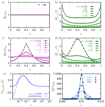
Figure 3: Statistics of the fraction of local-time $\theta_{x}(t)$ as a function of $x$ at different times $t$ for equilibrium initial conditions, $p_{0}(x_{0})=P_{\mathrm{inv}}(x_{0})$, (a and b) and localized initial condition at $x_{0}=0.405$ (c and d); a) $\langle\theta_{x}(t)\rangle_{\mathrm{inv}}$ is constant for all times; b) $\sigma_{\theta_{x},\mathrm{inv}}^{2}(t)$ as a function of $x$ for equilibrium initial conditions; c) $\langle\theta_{x}(t)\rangle_{x_{0}}$ and d) $\sigma_{\theta_{x}}^{2}(t)$; e) covariance starting from equilibrated initial conditions, $C_{\theta_{x}\theta_{y}}^{\mathrm{inv}}(t)$, (dashed line) and localized initial conditions, $C_{\theta_{x}\theta_{y}}(t)$ (solid line). f) Probability density of occupation time fraction $\theta_{\mathcal{V}}(t)=t^{-1}\int_{0}^{t}\mathbbm{1}_{[0.45,0.55]}(x_{\tau})d\tau$ (see also Eq. (7)) on large deviation time-scales (symbols) and corresponding theoretical result (56) (lines). Symbols were obtained from Brownian dynamics simulations of $10^{5}$ trajectories simulated with a time-step $dt=10^{-4}$.

Notably, starting from localized conditions $\langle\theta_{x}(t)\rangle_{x_{0}}$ as a function of $x$, in contrast to the ensemble propagator $P_{t}^{\mathrm{W}}(x|x_{0})$, displays a persistent cusp located at the initial condition $x_{0}$ (see Fig. 3 c). The fluctuations of $\theta_{x}(t)$ are larger near the initial condition and at the boundaries. Note that the fluctuations are always larger for equilibrium initial conditions (compare Fig. 3b and Fig. 3d).

V.2 Local time fraction of the Ornstein-Uhlenbeck process

Trajectories of the one-dimensional Ornstein-Uhlenbeck process are solutions of the Itô equation

$$dx_{t}=-\gamma x_{t}+\sqrt{2D}dW_{t}$$ (66)

and on the level or probability density correspond to the Fokker-Planck equation $(\partial_{t}-D[\partial^{2}_{x}+\gamma\partial_{x}x])P^{\mathrm{OU}}_{t}(x|x_{0})=0$ with initial condition $P^{\mathrm{OU}}_{0}(x|x_{0})=\delta(x-x_{0})$ and natural boundary conditions $\lim_{|x|\to\infty}P^{\mathrm{OU}}_{t}(x|x_{0})=0$. To connect continuous processes to discrete ones we translate the Fokker-Planck equation of the Ornstein-Uhlenbeck process to a random walk on a lattice with spacing $\Delta x$ and the harmonic potential $\gamma x^{2}$ entering transition rates according to Holubec et al. (2019)

$$\langle x+\Delta x|\hat{L}|x\rangle = \frac{D}{\Delta x^{2}}\mathrm{e}^{\frac{1}{4}\gamma[x^{2}-(x+\Delta x)^{2}]},$$

$$\langle x|\hat{L}|x+\Delta x\rangle = \frac{D}{\Delta x^{2}}\mathrm{e}^{\frac{1}{4}\gamma[(x+\Delta x)^{2}-x^{2}]},$$ (67)

in a confined domain $\Omega_{\rm conf}=\{-l,-l+\Delta x,\ldots,l-\Delta x,l\}\subset\Omega$. The matrix $\hat{L}$ is tri-diagonal and satisfies $\sum_{y}\langle y|\hat{L}|x\rangle=0$ for all $\mathbf{x}\in\Omega$ and $x\in\mathbb{Z}\Delta x$. We diagonalized $\hat{L}$ numerically using the library from Ref. Guennebaud et al. (2010). The mean, variance and correlation function for the continuous-space Ornstein-Uhlenbeck process (66) obtained from Brownian dynamics simulations are depicted in Fig. 4 (symbols) and are in excellent agreement with the spectral-theoretic results for the corresponding lattice random walk approximation (67) (lines). In Fig. 4f we also investigate the full probability density function of the fraction of occupation time in the interval $x\in[0,0.01]$, i.e. $\theta_{\mathcal{V}}(t)=t^{-1}\int_{0}^{t}\mathbbm{1}_{[0,0.01]}[x(\tau)]d\tau$ (see Eq. (7), on large deviation time scales and compare it to the theoretical Gaussian prediction Eq. (51).

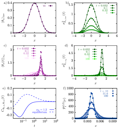
Figure 4: Statistics of the fraction of local-time $\theta_{x}(t)$ as a function of $x$ for the Ornstein Uhlenbeck process (symbols) and corresponding lattice random walk (67) with $10^{3}$ states in the interval $x\in[-5,5]$ as a function of $x$ at different times $t$ for equilibrium initial conditions, i.e. $p_{0}(x_{0})=P_{\mathrm{inv}}(x_{0})$ (a and b), and initial conditions localized at $x_{0}=1.2$ i.e. $p_{0}(x_{0})=\delta(x_{0}-1.2)$ (c and d). a) $\langle\theta_{x}(t)\rangle_{\mathrm{inv}}=P_{\mathrm{inv}}(x)$ is a time-independent Gaussian; b) $\sigma_{\theta_{x},\mathrm{inv}}^{2}(t)$ at various times as a function of $x$; c) $\langle\theta_{x}(t)\rangle_{x_{0}}$ and d) $\sigma_{\theta_{x},x_{0}}^{2}(t)$ at various times as a function of $x$; e) $C_{\theta_{0.5}\theta_{0.6}}(t)$ for equilibrium (dashed line) and localized (full lines) initial conditions; f) occupation time fraction $\theta_{\mathcal{V}}(t)=t^{-1}\int_{0}^{t}\mathbbm{1}_{[0,0.01]}[x(\tau)]d\tau$ (see also Eq. (7)) with symbols derived from simulations and the solid line representing the theoretical result (56) for the lattice random walk (67). To obtain each simulation point we generated $10^{5}$ Brownian dynamics trajectories using $D=\gamma=1$ with a time-step $dt=10^{-4}$.

Note that while the eigenspectrum of the generator of continuous Ornstein-Uhlenbeck dynamics is unbounded, implying that the spectral-theoretic result would require the summation of a large number of terms, the summation in the lattice approximation is limited by the number of lattice points. Therefore, except for very short times, where the lattice approximation naturally breaks down, this example demonstrates that our formalism applies equally well for Markov jump processes and diffusion dynamics. Note that the results in Fig. 4c,d for times $t=1$ and $t=100$ correspond to the “short” and “long” trajectory in Fig. 2, respectively.

V.3 Local time fraction in a driven uni-cyclic network

Let us in the following address a simple 3-state model with broken detailed balance to also address driven systems. The model corresponds to a simple cycle with states $1,2$ and $3$, where all rates in a given direction are equal but each of them has the same forward/backward asymmetry. The model may represent, for example, a molecular motor such as the F1-ATPase driven by ATP hydrolysis Toyabe et al. (2011). The corresponding transition matrix of the model reads

$$\hat{L}=\left(\begin{array}[]{ccc}-3&1&2\\ 2&-3&1\\ 1&2&-3\end{array}\right),$$ (68)

and has eigenvalues $\lambda_{0}=0$, $\lambda_{1,2}=-9/2\pm{\rm i}\sqrt{3}/2$ and eigenvectors $|R_{0}\rangle=3^{-1}(1,1,1)^{T}$ and

$$|R_{1,2}\rangle=\frac{1}{3}\left(\frac{-3\sqrt{3}\pm{\rm i}}{\sqrt{3}\mp 5{\rm i}},\frac{2\sqrt{3}\pm 2{\rm i}}{\sqrt{3}\mp 5{\rm i}},1\right)^{T}.$$ (69)

As a result of broken detailed balance the eigenspectrum is complex. In Fig. 5 we analyze the mean (panel a), fluctuations (panel b) and correlation function (panel c) of the local time fraction $\theta_{x}(t)$ in the various states for non-equilibrium steady-state initial conditions (light blue lines) and conditions initially localized in state $x_{0}=2$, i.e. $|p_{0}\rangle=(0,1,0)^{T}$. The theoretical results (lines) show an excellent agreement with simulations (symbols) carried out using the Gillespie algorithm Gillespie (1977). We also confirm the Gaussian statistics of the local time fraction $\theta_{x}(t)$ from Eq. (56) in Fig. 5d.

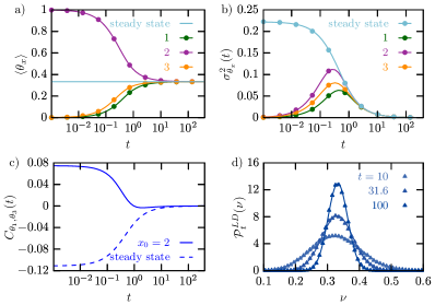
Figure 5: a) Mean local time fraction $\langle\theta_{x}(t)\rangle$ in states $x=1,2,3$ respectively, for a driven uni-cyclic network starting from steady-state initial conditions ($p_{0}(x_{0})=P_{\mathrm{inv}}(x_{0})$, light blue line; result identical for any state) and an initial condition localized at $x_{0}=2$ (lines are theory and points simulations); b) variance of the local time fraction $\sigma^{2}_{\theta,\mathrm{inv}}(t)$ starting from steady-state initial conditions (light blue line; result identical for any state) and $\sigma^{2}_{\theta,2}(t)$ in states $x=1,2,3$ starting from $x_{0}=2$; c) covariance of local time fraction between states $x=1$ and $x=2$, $C_{\theta_{1}\theta_{2}}(t)$, as a function of time for stationary (dashed line) and localized (full line) initial conditions; d) probability density function of the local time fraction in state $x=1$, $\overline{V}_{t}\equiv\theta_{1}(t)$, on large deviation time-scales alongside theoretical prediction of Eq. (56).

V.3.1 Generic behavior of local time fraction in ergodic systems

Note that an exhaustive study of the statistics of the local-time fraction is beyond the scope of this work. Nevertheless, we here discuss some general features of $\theta_{x}(t)$. The manner in which $\langle\theta_{x}(t)\rangle$, starting from some non-equilibrium initial condition, approaches the ergodic invariant measure $P_{\mathrm{inv}}(x)$ can be highly non-trivial and even non-monotonic (see e.g. Figs. 6a). Even when the ergodic limit is reached, where the variance ceases to depend on time, i.e. $t\sigma_{\theta_{x}}^{2}(t)\neq f(t)$, the fluctuations display a non-trivial behavior (see Fig. 6). For example, in the case of the Wiener process fluctuations are enhanced close to the boundaries, while for the Ornstein-Uhlenbeck process they become depressed near the minimum. Both results may be interpreted in terms of random ’oscillations’ around a typical position and confined by a boundary that amplifies fluctuations.

Figure 6: Long time behavior (i.e. $t\gg\lambda_{1}^{-1}$) of the scaled variance of the local-time, $t\sigma^{2}_{\theta_{x}}(t)$, that is time-independent; (a) results for the Wiener process and (b) the Ornstein-Uhlenbeck processes.

Moreover, the time-dependence of $\langle\theta_{x}(t)\rangle$ for non-stationary initial conditions is often non-monotonic or has a non-monotonic derivative (see Fig. 7a and c). A comparison between $\langle\theta_{x}(t)\rangle$ starting from stationary (dashed lines) and localized (full lines) initial conditions illustrates the two coexisting decorrelation mechanisms of $\theta_{x}(t)$ at different times, one corresponding to self-averaging and emergence of the central limit theorem (compare dashed and dotted lines), the other additionally reflecting the loss of memory of the initial condition (full lines). Stationary initial conditions always give rise to larger fluctuations than non-stationary initial conditions (compare dashed and full lines in Fig. 7b and d), and in the particular case of equilibrium initial conditions for systems obeying detailed balance, $\sigma^{2}_{\theta}(t)$ is a monotonically decaying function of time $t$ (see Eq. (52) and Fig. 7b and d) with an upper bound given by the large deviation asymptotic (see Eq. (61) with a $\propto 1/t$ scaling dictated by the central limit theorem (dotted lines in Fig. 7b and d).

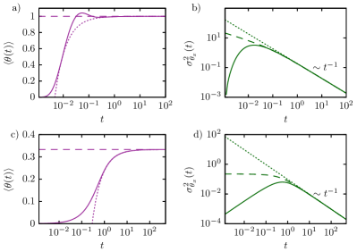
Figure 7: (a) Mean local-time and (b) variance at $x=0.6$ for a Wiener process starting from equilibrium (dashed line) and from a localized initial condition $p_{0}(x)=\delta(x-0.405)$ (solid line). (a) Mean local-time $\langle\theta_{x}(t)\rangle$ and (b) variance $\sigma^{2}_{\theta_{x}}(t)$ at $x=0.6$ for the driven 3-state cycle Eq. (68) starting from stationary (dashed line) and from a localized initial condition $p_{0}(x)=\delta(x-1)$ (solid line); The dotted lines correspond to the large deviation limit (51) and depict the validity and long-time saturation of the upper bound Eq. (61).

The covariance of the local time fraction between a pair of points $x_{1}$ and $x_{2}$ in the continuous setting (Figs. 3e and 4e) or $x=1$ and $x=2$ in the discrete setting (Fig. 5c), $C_{\theta_{1}\theta_{2}}(t)$, displays a similarly non-trivial and non-monotonic dependence on time and initial conditions $p_{0}(x_{0})$ as shown in Figs. 3e, 4e, and 5c. The striking dependence on the tagged points reflects a directional persistence of individual trajectories in-between said points and can therefore be used as a robust indicator of directional persistence and thus ’temporally correlated exploration’ on the level of a single trajectory.

V.3.2 Universal asymptotic Gaussian limit law for time-average physical observables

Finally, we comment on the universal asymptotic Gaussian limit law Eq. (56) for Markovian as well as non-Markovian time-average physical observables of type (3) of ergodic stochastic dynamics of the form given in Eqs. (14) and (26). Namely, using the asymptotic results (47), (51), and (55) in the large-deviation probability density function (56), and rescaling to the centered and time-independent variables $\Xi$ and $\Xi_{i|j}$ defined in Eqs. (57) and (58), we can rescale the probability density of any time-average physical observable $\mathcal{P}_{t}^{\mathrm{LD}}(\hat{\nu})$, and the conditional probability density of a time-average physical observable given another time-average physical observable $\mathcal{P}_{t}^{\mathrm{LD}}(\hat{\nu}_{i}|\hat{\nu}_{j})$, to collapse at long times onto a unit normal probability density (59). For the three models studied here, Figs. 3f, 4f, and 5d, and additionally for the conditional probability density function of occupation time fraction in $x\in[0.1,0.4]$ given occupation time fraction in $y\in[0.6,0.9]$ for the Wiener process, we demonstrate this collapse explicitly in Fig. 8.

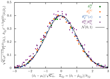
Figure 8: Collapse of probability density functions of all studied models at long time onto a unit normal probability density. The symbols correspond to rescaled probability density of occupation time fraction $\theta_{\mathcal{V}}(t)^{\mathrm{W,OU,cyc}}$ (see also Eq. (7)) of the Wiener process (64), the Ornstein-Uhlenbeck process (66), the driven 3-state cycle (68), respectively, and the conditional probability density function of occupation time fraction $\theta_{\mathcal{V}_{x}}(t)^{\mathrm{W}}|\theta_{\mathcal{V}_{y}}(t)^{\mathrm{W}}$ of the Wiener process for $\mathcal{V}_{x}=x\in[0.1,0.4]$ and $\mathcal{V}_{y}=y\in[0.6,0.9]$. The lines is a zero mean unit normal probability density function $\mathcal{N}(0,1)$.

V.4 Precision limit of concentration measurement by a single receptor

Let us now investigate the physical limit to the precision of concentrations measurements by means of the simplest two-state Markov jump process with states $\Omega=\{0,1\}$ Berg and Purcell (1977). The receptor can either be occupied by a ligand ($x=1$) or be empty ($x=0$). Let the background ligand concentration be $c$ and assume that the ligand binds with a rate $kc$ and unbinds with rate $k$, ignoring for simplicity any spatial variations of concentration. The generator and its eigenvectors are given by

$$\hat{L}=\begin{pmatrix}-kc&k\\ kc&-k\end{pmatrix},|R_{0}\rangle=\frac{1}{1+c}\begin{pmatrix}1\\ c\end{pmatrix},|R_{1}\rangle=\frac{1}{1+c}\begin{pmatrix}1\\ -1\end{pmatrix}$$ (70)

with $\lambda_{1}=-k(1+c)$ being the only non-zero eigenvalue. The left eigenvectors corresponding to Eq. (70) are $\langle L_{0}|=\langle-|=(1,1)$ and $\langle L_{1}|=(c,-1)$. Moreover, since the entire state space has only two states we have $\theta_{0}(t)=1-\theta_{1}(t)$. Assuming that the system was initially in equilibrium $|p_{0}\rangle=|R_{0}\rangle$ this implies that the mean values of the respective local time fractions are given by $\langle\theta_{1}(t)\rangle=(1+c)^{-1}c$ and $\langle\theta_{0}(t)\rangle=(1+c)^{-1}$.

If the receptor estimates the concentration $c$ by reading out and averaging the fraction of time the ligand is bound, $\theta_{1}$, over an interval of duration $t$, the precision of the estimate is bounded from above by the variance of the local time fraction given by Eq. (52) and reads explicitly

$$\sigma_{\theta_{1}}^{2}(t)=\frac{2c}{(1+c)^{3}kt}\bigg{[}1-\frac{1-\mathrm{e}^{-k(1+c)t}}{k(1+c)t}\bigg{]}.$$ (71)

Typically one assumes that the measurement $t$ is longer than any correlation time Berg and Purcell (1977); Bialek and Setayeshgar (2005); Godec and Metzler (2015, 2016), which in the present setting implies $t\gg 1/[k(1+c)]$, i.e. much longer than the correlation time of two-state Markov switching noise, $\tau_{c}\equiv\lambda_{1}^{-1}=1/(k+kc)$ Bialek and Setayeshgar (2005). In this regime the averaging-noise corresponds to shot-noise such that the variance decreases with the number of statistically independent receptor measurements $\#_{t}$ Berg and Purcell (1977); Bialek and Setayeshgar (2005); Godec and Metzler (2015, 2016), where $\#_{t}\sim t/\tau_{c}$ is the number of statistically independent realizations of the two-state process. Therefore $\sigma_{\theta_{1}}^{2}(t)\propto 1/\#_{t}=\tau_{c}/t$, according to the central limit theorem.

Based on the bound derived in Eq. (61) the shot-noise limit is in fact an upper bound to fluctuations of receptor occupancy at any duration of measurement, and saturates only in the limit $t\gg\tau_{c}$. Namely, a direct application of the bound (61) indeed yields, using $G^{\rm eq}_{t}(1,1)=P_{t}(1|1)P_{\infty}(1|1)$,

$$B \equiv 2\int_{0}^{\infty}[G^{\rm eq}_{t}(1,1)-G^{\rm eq}_{\infty}(1,1)]dt$$ (72)

$$= 2\int_{0}^{\infty}\frac{c}{(1+c)^{2}}\mathrm{e}^{-k(1+c)t}dt=\frac{2c}{(1+c)^{3}k},$$

implying, according to Eq. (61)

$$\sigma_{\theta_{1}}^{2}(t)\leq\frac{B}{t}=\frac{2c}{(1+c)^{2}}\frac{1}{\#_{t}}\equiv\lim_{t\gg\tau_{c}}\sigma_{\theta_{1}}^{2}(t).$$ (73)

Therefore, for short, and particularly finite measurements the shot-noise limit of fluctuations for long receptor read-out Berg and Purcell (1977); Bialek and Setayeshgar (2005); Godec and Metzler (2015, 2016) gives only an upper bound to the uncertainty of the estimate, whereas the inequality becomes sharp at long times.

Fundamental bounds on the precision of inferring $c$ from $\theta_{1}(t)$ can be found in Berg and Purcell (1977). Using the entire time trace of the receptor occupancy $x_{\tau}$ ($0\leq\tau\leq t$) instead of the occupation time $\theta_{1}(t)$ alone, and employing a maximum likelihood estimate of the concentration $c$, the error of the resulting estimate (i.e., its variance) is found to be reduced further by a factor of $1/2$ Endres and Wingreen (2009); Mora and Wingreen (2010). A detailed discussion of the precision of inferring kinetic parameters by means of non-local functionals can be found in Hartich and Seifert (2016).

VI Concluding perspective

We developed a general spectral-theoretic approach to time-average statistical mechanics, i.e. to the statistics of bounded, local additive functionals of (normal) ergodic stochastic processes with continuous and discrete state-spaces. In particular, we have shown how to obtain exactly the mean, variance and correlations of time-average observables from the eigenspectrum of the underlying forward or backward generator. We re-derived the famous Feynman-Kac formulas using Itô calculus and included a brief derivation for Markov-jump processes. We combined Feynman-Kac formulas with non-Hermitian perturbation theory to derive an exact spectral representation of the results. We demonstrated explicitly, and quantitatively, the emergence of the universal central limit law in a spectral representation on large deviation time-scales. For the special case of equilibrated initial conditions and dynamics obeying detailed balance we derived a general upper bound on fluctuations of occupation measures inferred from individual trajectories. We discussed our theoretical results from a physical perspective and provided simple but instructive practical examples to demonstrate how the theory is to be applied. Our work is applicable to continuous as well as discrete state-space processes, reversible as well as irreversible, encompassing a wide and diverse range of phenomena involving time-average observables and additive functionals in physical, chemical, and biological systems as well as financial mathematics and econophysics.

Appendix A The perturbative calculation

We carry out all calculations with the spectrum of the backward generator $\hat{L}^{\dagger}$. Equivalent results can be derived using the forward generator instead. We carry out perturbative calculations (34) up to second order to derive the results in Eq. (IV).

Terms of $1^{st}$ order in $u$

Starting with a perturbation of the backward ’kets’ and collecting terms of first order in Eq. (34) we find

$$-\hat{L}^{\dagger}|L_{k}^{1}\rangle+V|L_{k}\rangle=\lambda_{k}^{(1)}|L_{k}\rangle+\lambda^{\dagger}_{k}|L_{k}^{1}\rangle$$ (74)

and multiply Eq. (74) by $\langle R_{l}|$ from the left to obtain

$$-\langle R_{l}|\hat{L}^{\dagger}|L_{k}^{1}\rangle+\langle R_{l}|V|L_{k}\rangle=\lambda_{k}^{(1)}\delta_{kl}+\lambda^{\dagger}_{k}\langle R_{l}|L_{k}^{1}\rangle.$$ (75)

Therefore, if $k=l$ we find

$$\lambda_{k}^{(1)}=\langle R_{k}|V|L_{k}\rangle\equiv V_{kk}$$ (76)

while for $k\neq l$ we obtain

$$\langle R_{l}|L_{k}^{1}\rangle=\frac{V_{lk}}{\lambda^{\dagger}_{k}-\lambda^{\dagger}_{l}}$$ (77)

and therefore

$$|L_{k}^{1}\rangle=\sum_{l\neq k}\frac{V_{lk}}{\lambda^{\dagger}_{k}-\lambda^{\dagger}_{l}}|L_{l}\rangle.$$ (78)

We now turn to the perturbation of $\hat{L}^{\dagger}$ acting on the bra’s from the right and multiply the resulting first order equation by $|L_{l}\rangle$ from the right to obtain

$$-\langle R_{k}^{1}|\hat{L}^{\dagger}|L_{l}\rangle+\langle R_{k}|V|L_{l}\rangle=\lambda^{\dagger}_{k}\langle R_{k}^{1}|L_{l}\rangle+\lambda_{k}^{(1)}\delta_{kl}.$$ (79)

For $k=l$ we obtain the eigenvalue-corrections (76) while for $k\neq l$ we have

$$\langle R_{k}^{1}|=\sum_{l\neq k}\frac{V_{kl}}{\lambda^{\dagger}_{k}-\lambda^{\dagger}_{l}}\langle R_{l}|$$ (80)

Terms of $2^{nd}$ order in $u$

Collecting in Eq. (34) corrections of second order to the kets we find, upon multiplying by $\langle R_{l}|$ from the left,

$$-\langle R_{l}|\hat{L}^{\dagger}|L_{k}^{2}\rangle+\langle R_{l}|V|L_{k}^{1}\rangle$$

$$=\lambda_{k}^{(2)}\delta_{lk}+\lambda_{k}^{(1)}\langle R_{l}|L_{k}^{1}\rangle+\lambda^{\dagger}_{k}\langle R_{l}|L_{k}^{2}\rangle,$$ (81)

yielding, for $k=l$

$$\lambda_{k}^{(2)}=\langle R_{k}^{0}|\hat{V}|L_{k}^{1}\rangle,$$ (82)

because $\langle R_{k}|L_{k}^{1}\rangle=0$ due to the Eq. (36) and thus

$$\lambda_{k}^{(2)}=\sum_{l\neq k}\frac{V_{kl}V_{lk}}{\lambda^{\dagger}_{k}-\lambda^{\dagger}_{l}}\langle R_{l}|V|L_{k}\rangle.$$ (83)

Conversely, if $k\neq l$ we obtain the second order correction

$$|L_{k}^{2}\rangle=\sum_{l\neq k}\left[\sum_{i\neq k}\frac{V_{ik}V_{li}}{(\lambda^{\dagger}_{i}-\lambda^{\dagger}_{k})(\lambda^{\dagger}_{l}-\lambda^{\dagger}_{k})}-\frac{V_{kk}V_{lk}}{(\lambda^{\dagger}_{l}-\lambda^{\dagger}_{k})^{2}}\right]|L_{l}\rangle.$$ (84)

Collecting in Eq. (34) corrections of second order to the bra’s we find, upon multiplying from the right by $|L_{l}\rangle$

$$- \langle R_{k}^{2}|\hat{L}^{\dagger}|L_{l}\rangle+\langle R_{k}^{1}|V|L_{l}\rangle$$ (85)

$$= \lambda_{k}^{(2)}\delta_{kl}+\lambda_{k}^{(1)}\langle R_{k}^{1}|L_{l}\rangle+\lambda^{\dagger}_{k}\langle R_{k}^{2}|L_{l}\rangle.$$

When $k=l$ we obtain Eq. (83) while in the case when $k\neq l$ we find the second correction to the bra

$$\langle R_{k}^{2}|=\sum_{l\neq k}\left[\sum_{i\neq k}\frac{V_{ki}V_{il}}{(\lambda^{\dagger}_{i}-\lambda^{\dagger}_{k})(\lambda^{\dagger}_{l}-\lambda^{\dagger}_{k})}-\frac{V_{kk}V_{kl}}{(\lambda^{\dagger}_{l}-\lambda^{\dagger}_{k})^{2}}\right]\langle R_{l}|,$$ (86)

which completes the derivation of Eq. (IV).

Appendix B Derivation via the Dyson series

In a previous publication Lapolla and Godec (2018) we showed how to derive equations for the moments of $\psi_{t}$ for stationary initial conditions, $p_{0}(\mathbf{x})=P_{\mathrm{inv}}(\mathbf{x})$, (Eq. (52) and (54)) using a Dyson series approach. Here we sketch how to obtain the moments of $\psi_{t}$ for generic initial conditions $p_{0}(\mathbf{x})$. In contrast to Ref. Lapolla and Godec (2018) we here use the forward-approach and expand the tilted propagator up to the second order in $u$

$$\langle-|\mathrm{e}^{(\hat{L}-uV)t}|p_{0}\rangle=1-u\langle-|\int_{0}^{t}dt^{\prime}\mathrm{e}^{\hat{L}(t-t^{\prime})}V\mathrm{e}^{\hat{L}t^{\prime}}|p_{0}\rangle\\ +u^{2}\langle-|\int_{0}^{t}dt^{\prime}\int_{0}^{t^{\prime}}dt^{\prime\prime}\mathrm{e}^{\hat{L}(t-t^{\prime})}V\mathrm{e}^{\hat{L}(t^{\prime}-t^{\prime\prime})}V\mathrm{e}^{\hat{L}t^{\prime\prime}}|p_{0}\rangle\\ +\mathcal{O}(u^{3}),$$ (87)

assuming $t>t^{\prime}>t^{\prime\prime}>0$. Here we confirm that the Dyson series gives results identical to the perturbation-calculation.

Mean, fluctuations and correlations

We now derive $\langle\overline{V}_{t}\rangle$, $\sigma^{2}_{\overline{V}}(t)$ and $C_{\overline{V}_{1}\overline{V}_{2}}(t)$ presented in Eqs. (46)-(54) using the Dyson series. Note that this calculation does not diagonalize the tilted generator $\hat{L}^{\dagger}-uV(\mathbf{x})$ ($\hat{L}^{\dagger}-uV(\mathbf{x})$, respectively). Starting form Eq. (87) we can carry out all integrations analytically for arbitrary initial conditions $p_{0}(\mathbf{x})$. To first order in $u$ we obtain

$$t^{-1}\langle-|\int_{0}^{t}dt^{\prime}\mathrm{e}^{\hat{L}(t-t^{\prime})}V\mathrm{e}^{\hat{L}t^{\prime}}|p_{0}\rangle$$ (88)

$$= t^{-1}\int_{0}^{t}dt^{\prime}\sum_{k}\sum_{l}\langle-|R_{l}\rangle\langle L_{l}|V|R_{k}\rangle\langle L_{k}|p_{0}\rangle\mathrm{e}^{-\lambda_{l}(t-t^{\prime})-\lambda_{k}t^{\prime}}$$

$$= t^{-1}\int_{0}^{t}dt^{\prime}\sum_{k}\langle-|V|R_{k}\rangle\langle L_{k}|p_{0}\rangle\mathrm{e}^{-\lambda_{k}t^{\prime}}$$

$$= V_{00}+\frac{1}{t}\sum_{k}\frac{V_{k0}}{\lambda_{k}}\langle L_{k}|p_{0}\rangle(1-\mathrm{e}^{-\lambda_{k}t}),$$

where for $p_{0}(\mathbf{x})=P_{\mathrm{inv}}(\mathbf{x})$ we have $\langle L_{k}|p_{0}\rangle=\delta_{k0}$ leading to $\langle\overline{V}\rangle_{\mathrm{inv}}=V_{00}=P_{\mathrm{inv}}(\mathbf{x})$.

To second order in $u$ we find for an arbitrary $p_{0}(\mathbf{x})$

$$t^{-2}\langle-|\int_{0}^{t}dt^{\prime}\int_{0}^{t^{\prime}}dt^{\prime\prime}\mathrm{e}^{\hat{L}(t-t^{\prime})}V\mathrm{e}^{\hat{L}(t^{\prime}-t^{\prime\prime})}V\mathrm{e}^{\hat{L}t^{\prime\prime}}|p_{0}\rangle$$ (89)

$$= t^{-2}\int_{0}^{t}dt^{\prime}\int_{0}^{t^{\prime}}dt^{\prime\prime}\langle-|\sum_{m}|R_{m}\rangle\langle L_{m}|\mathrm{e}^{-\lambda_{m}(t-t^{\prime})}V\sum_{k}|R_{k}\rangle\langle L_{k}|\mathrm{e}^{-\lambda_{k}(t^{\prime}-t^{\prime\prime})}V\sum_{l}|R_{i}\rangle\langle L_{l}|\mathrm{e}^{-\lambda_{l}t^{\prime\prime}}|p_{0}\rangle$$

$$= t^{-2}\sum_{k}\sum_{l}V_{0k}V_{kl}\langle L_{l}|p_{0}\rangle\int_{0}^{t}dt^{\prime}\int_{0}^{t^{\prime}}dt^{\prime\prime}\mathrm{e}^{-\lambda_{k}(t^{\prime}-t^{\prime\prime})-\lambda_{l}t^{\prime\prime}};$$

when $k=l=0$ only $V_{00}^{2}/2$ survives, while for $k\neq 0$ and $l=0$ we find

$$\frac{1}{t}\sum_{k>0}\frac{V_{k0}V_{0k}}{\lambda_{k}}\left(1-\frac{1-\mathrm{e}^{-\lambda_{k}t}}{t\lambda_{k}}\right).$$ (90)

Conversely, when $k=0$ and $l\neq 0$ we end up with

$$\frac{1}{t}\sum_{l>0}\frac{V_{00}V_{l0}}{\lambda_{l}}\langle L_{l}|p_{0}\rangle\left(1-\frac{1-\mathrm{e}^{-\lambda_{l}t}}{t\lambda_{l}}\right),$$ (91)

while for $k=l$ and $k\neq 0$ and $l\neq 0$ we have

$$\frac{1}{t}\sum_{k>0}\frac{V_{k0}V_{kk}}{\lambda_{k}}\langle L_{k}|p_{0}\rangle\left(\mathrm{e}^{-\lambda_{k}t}-\frac{1-\mathrm{e}^{-\lambda_{k}t}}{t\lambda_{k}}\right).$$ (92)

Finally, when $k\neq l\neq 0$ we obtain

$$\frac{1}{t^{2}}\sum_{k>0}\sum_{l>0,l\neq k}\frac{V_{k0}V_{lk}}{\lambda_{k}-\lambda_{l}}\langle L_{l}|p_{0}\rangle\left(\frac{1-\mathrm{e}^{-\lambda_{l}t}}{\lambda_{l}}-\frac{1-\mathrm{e}^{-\lambda_{k}t}}{\lambda_{k}}\right)$$ (93)

The sum of these terms yields the result sought for. The corresponding result for stationary initial conditions, $p_{0}(\mathbf{x})=P_{\mathrm{inv}}(\mathbf{x})$, is obtained using $\langle L_{l}|P_{\mathrm{inv}}\rangle=\delta_{l0}$, which leads to Eq. (52) and (54). When considering correlations we make the replacement $uV\to u_{1}V_{1}+u_{2}V_{2}$ and replace $\partial^{2}_{u_{1}}\to\partial^{2}_{u_{1}u_{2}}$ to compute the covariance. The formulas above thereby generalize in a straightforward manner.

References

- Saxton (2008) M. J. Saxton, Nat. Methods 5, 671 (2008).
- Metzler et al. (2014) R. Metzler, J.-H. Jeon, A. G. Cherstvy, and E. Barkai, Phys. Chem. Chem. Phys. 16, 24128 (2014).
- Ernst et al. (2014) D. Ernst, J. Köhler, and M. Weiss, Phys. Chem. Chem. Phys. 16, 7686 (2014).
- Shen et al. (2017) H. Shen, L. J. Tauzin, R. Baiyasi, W. Wang, N. Moringo, B. Shuang, and C. F. Landes, Chem. Rev. 117, 7331 (2017).
- Hughes and Dougan (2016) M. L. Hughes and L. Dougan, Rep. Prog. Phys. 79, 076601 (2016).
- Xie (1996) X. S. Xie, Acc. Chem. Res. 29, 598 (1996).
- Ambrose et al. (1999) W. P. Ambrose, P. M. Goodwin, J. H. Jett, A. Van Orden, J. H. Werner, and R. A. Keller, Chem. Rev. 99, 2929 (1999).
- Plakhotnik et al. (1997) T. Plakhotnik, E. A. Donley, and U. P. Wild, Annu. Rev. Phys. Chem. 48, 181 (1997).
- Neuman and Nagy (2008) K. C. Neuman and A. Nagy, Nat. Methods 5, 491 (2008).
- Rief and Grubmüller (2002) M. Rief and H. Grubmüller, ChemPhysChem 3, 255 (2002).
- Woodside and Block (2014) M. T. Woodside and S. M. Block, Annu. Rev. Biophys. 43, 19 (2014).
- Ritort (2006) F. Ritort, J. Phys.: Condens. Matter 18, R531 (2006).
- Camunas-Soler et al. (2016) J. Camunas-Soler, M. Ribezzi-Crivellari, and F. Ritort, Annu. Rev. Biophys. 45, 65 (2016).
- Lévy (1940) P. Lévy, Compositio Mathematica 7, 283 (1940).
- Kac (1949) M. Kac, Trans. Amer. Math. Soc. 65, 1 (1949).
- Darling and Kac (1957) D. A. Darling and M. Kac, Trans. Am. Math. Soc. 84, 444 (1957).
- Lamperti (1958) J. Lamperti, Trans. Amer. Math. Soc. 88, 380 (1958).
- Feller (1949) W. Feller, Trans. Am. Math. Soc. 67, 98 (1949).
- Bingham (1975) N. H. Bingham, Adv. Appl. Probab. 7, 705 (1975).
- Borodin (1989) A. N. Borodin, Russ. Math. Surv. 44, 1 (1989).
- Yen and Yor (2013) J.-Y. Yen and M. Yor, Lect. Notes Math. (2013), 10.1007/978-3-319-01270-4.
- Yor (2001) M. Yor, Exponential Functionals of Brownian Motion and Related Processes, Springer Finance Lecture Notes (Springer-Verlag, Berlin Heidelberg, 2001).
- Geman and Yor (1993) H. Geman and M. Yor, Mathematical Finance 3, 349 (1993).
- Wilemski and Fixman (1973) G. Wilemski and M. Fixman, J. Chem. Phys. 58, 4009 (1973).
- Szabo (1989) A. Szabo, J. Phys. Chem. 93, 6929 (1989).
- Bénichou et al. (2005) O. Bénichou, M. Coppey, M. Moreau, and G. Oshanin, J. Chem. Phys. 123, 194506 (2005).
- Grebenkov (2007) D. S. Grebenkov, Phys. Rev. E 76, 041139 (2007).
- Berg and Purcell (1977) H. C. Berg and E. M. Purcell, Biophys. J. 20, 193 (1977).
- Wiegel (1983) F. Wiegel, Phys. Rep. 95, 283 (1983).
- Bialek and Setayeshgar (2005) W. Bialek and S. Setayeshgar, Proc. Natl. Acad. Sci. USA 102, 10040 (2005).
- Endres and Wingreen (2009) R. G. Endres and N. S. Wingreen, Phys. Rev. Lett. 103, 158101 (2009).
- Mora and Wingreen (2010) T. Mora and N. S. Wingreen, Phys. Rev. Lett. 104, 248101 (2010).
- Lang et al. (2014) A. H. Lang, C. K. Fisher, T. Mora, and P. Mehta, Phys. Rev. Lett. 113, 148103 (2014).
- Mora (2015) T. Mora, Phys. Rev. Lett. 115, 038102 (2015).
- Barato and Seifert (2015) A. C. Barato and U. Seifert, Phys. Rev. E 92, 032127 (2015).
- Aquino et al. (2015) G. Aquino, N. S. Wingreen, and R. G. Endres, J. Stat. Phys. 162, 1353 (2015).
- Hartich and Seifert (2016) D. Hartich and U. Seifert, Phys. Rev. E 94, 042416 (2016).
- Ferraro and Zaninetti (2004) M. Ferraro and L. Zaninetti, Physica A 338, 307 (2004).
- Gandjbakhche and Weiss (2000) A. H. Gandjbakhche and G. H. Weiss, Phys. Rev. E 61, 6958 (2000).
- Weiss and Calabrese (1996) G. H. Weiss and P. P. Calabrese, Physica A 234, 443 (1996).
- Toroczkai et al. (1999) Z. Toroczkai, T. J. Newman, and S. Das Sarma, Phys. Rev. E 60, R1115 (1999).
- Brokmann et al. (2003) X. Brokmann, J.-P. Hermier, G. Messin, P. Desbiolles, J.-P. Bouchaud, and M. Dahan, Phys. Rev. Lett. 90, 120601 (2003).
- Stefani et al. (2009) F. D. Stefani, J. P. Hoogenboom, and E. Barkai, Phys. Today 62, 34 (2009).
- Comtet et al. (2005) A. Comtet, J. Desbois, and C. Texier, J. Phys. A: Math. Gen. 38, R341 (2005).
- Majumdar and Bray (2002) S. N. Majumdar and A. J. Bray, Phys. Rev. E 65, 051112 (2002).
- Majumdar, Satya N. (2005) Majumdar, Satya N., Curr. Sci. 89, 2079 (2005).
- Wennmalm et al. (1997) S. Wennmalm, L. Edman, and R. Rigler, Proc. Natl. Acad. Sci. USA 94, 10641 (1997).
- Gopich and Szabo (2012) I. V. Gopich and A. Szabo, Proc. Natl. Acad. Sci. USA 109, 7747 (2012).
- Fleury et al. (2000) L. Fleury, J.-M. Segura, G. Zumofen, B. Hecht, and U. P. Wild, Phys. Rev. Lett. 84, 1148 (2000).
- Barkai et al. (2004) E. Barkai, Y. Jung, and R. Silbey, Annu. Rev. Phys. Chem. 55, 457 (2004).
- Agmon (2010) N. Agmon, Chem. Phys. Lett. 497, 184 (2010).
- Sabhapandit et al. (2006) S. Sabhapandit, S. N. Majumdar, and A. Comtet, Phys. Rev. E 73, 051102 (2006).
- Majumdar and Comtet (2002) S. N. Majumdar and A. Comtet, Phys. Rev. Lett. 89, 060601 (2002).
- Bel and Barkai (2005) G. Bel and E. Barkai, Phys. Rev. Lett. 94, 240602 (2005).
- Carmi and Barkai (2011) S. Carmi and E. Barkai, Phys. Rev. E 84, 061104 (2011).
- Dhar and Majumdar (1999) A. Dhar and S. N. Majumdar, Phys. Rev. E 59, 6413 (1999).
- Majumdar and Dean (2002) S. N. Majumdar and D. S. Dean, Phys. Rev. E 66, 041102 (2002).
- Bray et al. (2013) A. J. Bray, S. N. Majumdar, and G. Schehr, Adv. Phys. 62, 225 (2013).
- Lapolla and Godec (2018) A. Lapolla and A. Godec, New J. Phys. 20, 113021 (2018).
- Lapolla and Godec (2019) A. Lapolla and A. Godec, Front. Phys. 7, 182 (2019).
- Boyer et al. (2012a) D. Boyer, D. S. Dean, C. Mejía-Monasterio, and G. Oshanin, Phys. Rev. E 86, 060101 (2012a).
- Boyer et al. (2012b) D. Boyer, D. S. Dean, C. Mejía-Monasterio, and G. Oshanin, Phys. Rev. E 85, 031136 (2012b).
- Jørgensen et al. (2005) J. B. Jørgensen, J. Mann, S. Ott, H. L. Pécseli, and J. Trulsen, Phys. Fluids 17, 035111 (2005).
- Barato and Chetrite (2015) A. Barato and R. Chetrite, J. Stat. Phys. 160, 1154 (2015).
- Touchette (2009) H. Touchette, Phys. Rep. 478, 1 (2009).
- Touchette (2018) H. Touchette, Physica A 504, 5 (2018), lecture Notes of the 14th International Summer School on Fundamental Problems in Statistical Physics.
- Gardiner (2004) C. W. Gardiner, Handbook of Stochastic Methods, 3rd ed. (Springer, Berlin, 2004).
- Gillespie (1977) D. T. Gillespie, J. Phys. Chem. 81, 2340 (1977).
- Schnakenberg (1976) J. Schnakenberg, Rev. Mod. Phys. 48, 571 (1976).
- Conway (1985) J. B. Conway, A Course in Functional Analysis, Graduate Texts in Mathematics (Springer-Verlag, New York, 1985).
- van Kampen (2007) N. G. van Kampen, Stochastic Processes in Physics and Chemistry, 3rd ed., North-Holland Personal Library (Elsevier, Amsterdam, 2007).
- Risken (1996) H. Risken, The Fokker-Planck Equation: Methods of Solution and Applications, 2nd ed., Springer Series in Synergetics (Springer-Verlag, Berlin Heidelberg, 1996).
- Stoller et al. (1991) S. D. Stoller, W. Happer, and F. J. Dyson, Phys. Rev. A 44, 7459 (1991).
- Note (1) Note that is an eigenvalue of and is meromorphic for small therefore we can assume, without loss of generality, that is real.
- Marcinkiewicz (1939) J. Marcinkiewicz, Math. Z. 44, 612 (1939).
- Sakurai and Napolitano (2017) J. J. Sakurai and J. Napolitano, Modern Quantum Mechanics (Cambridge University Press, 2017).
- Klein (1974) D. J. Klein, J. Chem. Phys. 61, 786 (1974).
- Hartich and Godec (2019) D. Hartich and A. Godec, J. Phys. A: Math. Theor. 52, 244001 (2019).
- Khinchin (1929) A. I. Khinchin, Comptes rendus de l’Academie des Sciences 189, 477 (1929).
- Holubec et al. (2019) V. Holubec, K. Kroy, and S. Steffenoni, Phys. Rev. E 99, 032117 (2019).
- Guennebaud et al. (2010) G. Guennebaud, B. Jacob, et al., “Eigen v3,” http://eigen.tuxfamily.org (2010).
- Toyabe et al. (2011) S. Toyabe, T. Watanabe-Nakayama, T. Okamoto, S. Kudo, and E. Muneyuki, Proc. Natl. Acad. Sci. USA 108, 17951 (2011).
- Godec and Metzler (2015) A. Godec and R. Metzler, Phys. Rev. E 92, 010701 (2015).
- Godec and Metzler (2016) A. Godec and R. Metzler, J. Phys. A: Math. Theor. 49, 364001 (2016).