Multipolar Effective-One-Body Waveforms for Precessing Binary Black Holes:
Construction and Validation
Abstract
As gravitational-wave detectors become more sensitive and broaden their frequency bandwidth,
we will access a greater variety of signals emitted by compact binary systems, shedding light on their
astrophysical origin and environment. A key physical effect that can distinguish among different
formation scenarios is the misalignment of the spins with the orbital angular momentum, causing the spins
and the binary’s orbital plane to precess. To accurately model such precessing signals, especially
when masses and spins vary in the wide astrophysical range, it is crucial to include multipoles
beyond the dominant quadrupole. Here, we develop the first multipolar precessing waveform model
in the effective-one-body (EOB) formalism for the entire coalescence stage (i.e., inspiral,
merger and ringdown) of binary black holes: SEOBNRv4PHM. In the nonprecessing limit, the model reduces to
SEOBNRv4HM, which was calibrated to numerical-relativity (NR) simulations, and
waveforms from black-hole perturbation theory.
We validate the SEOBNRv4PHM by comparing it to the public catalog of 1405 precessing NR waveforms
of the Simulating eXtreme Spacetimes (SXS) collaboration, and also to 118 SXS precessing NR waveforms,
produced as part of this project, which span mass ratios 1-4 and (dimensionless) black-hole’s spins
up to 0.9. We stress that SEOBNRv4PHM is not calibrated to NR simulations in the
precessing sector. We compute the unfaithfulness against
the 1523 SXS precessing NR waveforms, and find that, for ( ) of the cases, the maximum value, in the
total mass range , is below (). Those numbers change to ( )
when using the inspiral-merger-ringdown, multipolar, precessing phenomenological model IMRPhenomPv3HM.
We investigate the impact of such unfaithfulness values with two Bayesian, parameter-estimation studies on synthetic signals.
We also compute the unfaithfulness between
those waveform models as a function of the mass and spin parameters to identify in which part of the parameter
space they differ the most. We validate them also against the multipolar, precessing NR surrogate model NRSur7dq4,
and find that the SEOBNRv4PHM model outperforms IMRPhenomPv3HM.
pacs:
04.25.D-, 04.25.dg, 04.30.-wI Introduction
Since the Laser Interferometer Gravitational wave Observatory (LIGO) detected a gravitational wave (GWs) from a binary–black-hole (BBH) in 2015 Abbott et al. (2016a), multiple observations of GWs from BBHs have been made with the LIGO Aasi et al. (2015) and Virgo Acernese et al. (2015) detectors Abbott et al. (2016b); Abbott et al. (2019); Zackay et al. (2019); Venumadhav et al. (2019); Nitz et al. (2019). Two binary neutron star (BNSs) systems have been observed Abbott et al. (2017a); Abbott et al. (2020), one of them both in gravitational and electromagnetic radiation Abbott et al. (2017b, c), opening the exciting new chapter of multi-messenger GW astronomy. Mergers of compact-object binaries are expected to be detected at an even higher rate with LIGO and Virgo ongoing and future, observing runs Abbott et al. (2018), and with subsequent third-generation detectors on the ground, such as the Einstein Telescope and Cosmic Explorer, and the Laser Interferometer Space Antenna (LISA). In order to extract the maximum amount of astrophysical and cosmological information, the accurate modeling of GWs from binary systems is more critical than ever. Great progress has been made in this direction, both through the development of analytical methods to solve the two-body problem in General Relativity (GR), and by ever-more expansive numerical-relativity (NR) simulations.
One of the key areas of interest is to improve the modeling of systems where the misalignment of the spins with the orbital angular momentum causes the spins and the orbital plane to precess Apostolatos et al. (1994). Moreover, when the binary’s component masses are asymmetric, gravitational radiation is no longer dominated by the quadrupole moment, and higher multipoles need to be accurately modeled Blanchet (2014). Precession and higher multipoles lead to very rich dynamics, which in turn is imprinted on the GW signal. Their measurements will be able to shed light on the formation mechanism of the observed systems, probe the astrophysical environment, break degeneracy among parameters, allowing more accurate measurements of cosmological parameters, masses and spins, and more sophisticated tests of GR.
Faithful waveform models for precessing compact-object binaries have been developed within the
effective-one-body (EOB) formalism Taracchini et al. (2013); Pan et al. (2014); Babak et al. (2017),
and the phenomenological approach Hannam et al. (2014); Khan et al. (2016, 2019); Pratten
et al. (2020a); García-Quirós
et al. (2020) through calibration
to NR simulations. Recently, an inspiral-merger-ringdown phenomenological waveform model that tracks precession and
includes higher modes was constructed in Ref. Khan et al. (2020) (henceforth, IMRPhenomPv3HM) 111During the final preparation of this work, a new frequency-domain phenomenological model with precession and higher modes (IMRPhenomXPHM Pratten et al. (2020b)), and a time-domain phenomenological precessing model with the dominant mode (IMRPhenomTP Estellés et al. (2020)) were developed. We leave the comparison to these models for future work.
The model describes the six spin degrees of freedom in the inspiral phase, but not in the late-inspiral, merger and ringdown stages.
In the co-precessing frame Buonanno et al. (2003); Schmidt et al. (2011); Boyle et al. (2011); O’Shaughnessy et al. (2011); Schmidt et al. (2012),
in which the BBH is viewed face-on at all times and the GW radiation resembles the
nonprecessing one, it includes the modes and . Here, building on the multipolar
aligned-spin EOB waveform model of Ref. Bohé et al. (2017); Cotesta et al. (2018),
which was calibrated to 157 NR simulations Mroue et al. (2013); Chu et al. (2016), and 13 waveforms from
BH perturbation theory for the (plunge-)merger and ringdown Barausse et al. (2012), we develop the first EOB waveform model that
includes both spin-precession and higher modes (henceforth, SEOBNRv4PHM). The model describes
the six spin degrees of freedom throughout the BBH coalescence. It differs from the one
of Refs. Pan et al. (2014); Babak et al. (2017), not only because it includes in the co-precessing
frame the , and
modes, beyond the and modes, but also because it uses an improved description
of the two-body dynamics, having been calibrated Bohé et al. (2017) to a large set of NR waveforms Mroue et al. (2013). We note that IMRPhenomPv3HM and SEOBNRv4PHM are not completely independent
because the former is constructed fitting (in frequency domain) hybridized waveforms obtained by stitching together EOB and NR waveforms.
We stress that both SEOBNRv4HM and IMRPhenomPv3HM are not calibrated to NR simulations in the
precessing sector. Finally, the surrogate approach, which interpolates NR waveforms, has been used to construct several waveform models that include higher modes Varma et al. (2019a) and precession Blackman et al. (2017). In this paper, we consider the state-of-the-art surrogate waveform model with full spin precession and higher modes Varma et al. (2019b) (henceforth, NRSur7dq4),
developed for binaries with mass ratios 1-4, (dimensionless) BH’s spins up to and binary’s
total masses larger than . It includes in the co-precessing frame all modes up to .
Table 1 summarizes the waveform models used in this paper.
| Model name | Modes in the co-precessing frame | Reference |
|---|---|---|
| SEOBNRv3P | , | Pan et al. (2014); Babak et al. (2017) |
| SEOBNRv4P | , | this work |
| SEOBNRv4PHM | , , , | |
| this work | ||
| IMRPhenomPv2 | Hannam et al. (2014) | |
| IMRPhenomPv3 | Khan et al. (2019) | |
| IMRPhenomPv3HM | , , , , | |
| , | Khan et al. (2020) | |
| NRSur7dq4 | all with | Varma et al. (2019b) |
The best tool at our disposal to validate waveform models built from approximate solutions of the Einstein equations, such as the ones obtained from post-Newtonian (PN) theory, BH perturbation theory and the EOB approach, is their comparison to NR waveforms. So far, NR simulations of BBHs have been mostly limited to mass ratio and (dimensionless) spins , and length of orbital cycles before merger Jani et al. (2016); Healy et al. (2017, 2019); Huerta et al. (2019); Boyle et al. (2019) (however, see Ref. Hinder et al. (2019) where simulations with larger spins and mass ratios were obtained through a synergistic use of NR codes). Here, to test our newly constructed EOB precessing waveform model, we enhance the NR parameter-space coverage, while maintaining a manageable computational cost, and perform new NR simulations with the pseudo spectral Einstein code (SpEC) of the Simulating eXtreme Spacetimes (SXS) collaboration. The new NR simulations span BBHs with mass ratios , and dimensionless spins in the range , and different spins’ orientations. To assess the accuracy of the different precessing waveform models, we compare them to the NR waveforms of the public SXS catalogue Boyle et al. (2019), and to the new NR waveforms produced for this paper.
The paper is organized as follows. In Sec. II we discuss the new NR simulations of BBHs,
and assess their numerical error. In Sec. III we develop the multipolar EOB waveform
model for spin-precessing BBHs, SEOBNRv4PHM, and highlight the improvements with respect to the
previous version Pan et al. (2014); Babak et al. (2017), which was used in LIGO and Virgo
inference analyses Abbott et al. (2016c, 2017d, 2019).
In Sec. IV we validate the accuracy of the multipolar precessing EOB model
by comparing it to NR waveforms. We also compare the performance of SEOBNRv4PHM
against the one of IMRPhenomPv3HM, and study in which region of the parameter space
those models differ the most from NR simulations, and also from each other. In Sec. V
we use Bayesian analysis to explore the impact of the accuracy of the precessing waveform models
when extracting astrophysical information and perform two synthetic NR injections in zero noise.
In Sec. VI we summarize our main conclusions and discuss future work. Finally,
in Appendix A we compare the precessing waveform models to the
NR surrogate NRSur7dq4, and in Appendix B we list the parameters
of the 118 NR simulations done for this paper.
In what follows, we use geometric units unless otherwise specified.
II New numerical-relativity simulations of spinning, precessing binary black holes
Henceforth, we denote with the two BH masses (with ), their spins, the mass ratio, the binary’s total mass, the reduced mass, and the symmetric mass ratio. We indicate with the total angular momentum, where and , are the orbital angular momentum and the total spin, respectively
II.1 New precessing numerical-relativity waveforms

The spectral Einstein code (SpEC) 222www.black-holes.org of the Simulating eXtreme Spacetimes (SXS) collaboration is a multi-domain collocation code designed for the solution of partial differential equations on domains with simple topologies. It has been used extensively to study the mergers of compact-object binaries composed of BH Scheel et al. (2015); Lovelace et al. (2015); Szilágyi et al. (2015); Lovelace et al. (2016); Afle et al. (2018); Boyle et al. (2019) and NSs Foucart et al. (2016); Haas et al. (2016); Foucart et al. (2019); Vincent et al. (2020), including in theories beyond GR Okounkova et al. (2019a, b, c); Okounkova (2020). SpEC employs a first-order symmetric-hyperbolic formulation of Einstein’s equations Lindblom et al. (2006) in the damped harmonic gauge Lindblom and Szilagyi (2009); Szilagyi et al. (2009). Dynamically controlled excision boundaries are used to treat spacetime singularities Hemberger et al. (2013); Scheel et al. (2015) (see Ref. Boyle et al. (2019) for a recent, detailed overview).
Significant progress has been made in recent years by several NR groups to improve the coverage of the BBH parameter space Jani et al. (2016); Healy et al. (2017, 2019); Huerta et al. (2019); Boyle et al. (2019); Hinder et al. (2019), mainly motivated by the calibration of analytical waveform models and surrogate models used in LIGO and Virgo data analysis. While large strides have been made for aligned-spin cases, the exploration of precessing waveforms has been mostly limited to , typically orbital cycles before merger, and a large region of parameter space remains to be explored. Simulations with high mass ratio () and high spin () are challenging, primarily due to the need to resolve the disparate length scales in the binary system, which increases the computational cost for a given level of accuracy. Furthermore, for high spin, the apparent horizons can be dramatically smaller, which makes it more difficult to control the excision boundaries, further increasing the computational burden.
Here, we want to improve the parameter-space coverage of the SXS catalog Boyle et al. (2019), while maintaining a manageable computational cost, thus we restrict to simulations in the range of mass ratios and (dimensionless) spins , with the spin magnitudes decreasing as the mass ratio increases. In Fig. 1 we display, in the parameter space, the precessing and non-precessing waveforms from the published SXS catalogue Boyle et al. (2019), and the new precessing waveforms produced as part of this work.
We choose to start all the simulations at the same (angular) orbital frequency, , where the value is not exact as it was modified slightly during the eccentricity-reduction procedure in SpEC Buonanno et al. (2011). This corresponds to a physical GW starting frequency of Hz at and results in the number of orbits up to merger varying between and in our new catalog.
We parametrize the directions of the spins by three angles, the angles between the spins and the unit vector along the Newtonian orbital angular momentum, , and the angle between the projections of the spins in the orbital plane. Explicitly,
| (1a) | ||||
| (1b) | ||||
where . We make the choice that lies in the plane, where is the unit vector along the binary’s radial separation, at the start of the simulation. The angles are chosen to be , and . Here is the angle that maximizes the opening angle of around the total angular momentum and is computed assuming that the two spins are co-linear, giving
| (2) |
with for circular orbit, being the orbital angular frequency. For each choice of we choose 10 different configurations divided into two categories: i) giving eight runs, and ii) giving two runs. The detailed parameters can be found in Appendix B.
These choices of the spin directions allow us to test the multipolar
precessing model SEOBNRv4PHM in many different regimes, including where the effects of
precession are maximized, and where spin-spin effects are significant or diminished.
II.2 Unfaithfulness for spinning, precessing waveforms
The gravitational signal emitted by non-eccentric BBH systems and observed by a detector depends on 15 parameters: the component masses and (or equivalently the mass ratio and the total mass ), the dimensionless spins and , the direction to observer from the source described by the angles , the luminosity distance , the polarization , the location in the sky and the time of arrival . The gravitational strain can be written as:
| (3) |
where to simplify the notation we introduce the function . The functions and are the antenna patterns Sathyaprakash and Dhurandhar (1991); Finn and Chernoff (1993):
| (4a) | ||||
| (4b) | ||||
Equation (II.2) can be rewritten as:
| (5) |
where is the effective polarization Capano et al. (2014) defined as:
| (6) |
which has support in the region , while reads:
| (7) |
Henceforth, to ease the notation we suppress the dependence on in .
Let us introduce the inner product between two waveforms and Sathyaprakash and Dhurandhar (1991); Finn and Chernoff (1993):
| (8) |
where a tilde indicates the Fourier transform, a star the complex conjugate and is the one-sided power spectral density (PSD) of the detector noise. We employ as PSD the Advanced LIGO’s “zero-detuned high-power” design sensitivity curve Barsotti et al. (2018). Here we use and , when both waveforms fill the band. For cases where this is not the case (e.g the NR waveforms) we set , where is the starting frequency of the waveform.
To assess the closeness between two waveforms (e.g., the signal) and (e.g., the template), as observed by a detector, we define the following faithfulness function Cotesta et al. (2018):
| (9) |
While in the equation above we set the inclination angle of signal and template waveforms to be the same, the coalescence time and the angles and of the template waveform are adjusted to maximize the faithfulness. This is a typical choice motivated by the fact these quantities are not interesting from an astrophysical perspective. The maximizations over and are performed numerically, while the maximization over is done analytically following the procedure described in Ref. Capano et al. (2014) (see Appendix A therein).
The condition in Eq. (9) enforces that the mass
ratio , the total mass and the spins of the
template waveform at (i.e., at the beginning of the
waveform) are set to have the same values of the ones in the signal
waveform at its . When computing the faithfulness between NR
waveforms with different resolutions this condition is trivially
satisfied by the fact that they are generated using the same initial
data. In the case of the faithfulness between NR and any model from the SEOBNR family, it
is first required to ensure that has the same physical meaning
for both waveforms. Ideally in the SEOBNR
waveform should be fixed by requesting that the frequency of the SEOBNR
mode at coincides with the NR (2,2) mode
frequency at . This is in practice not possible
because the NR (2,2) mode frequency may display small oscillations
caused by different effects — for example the persistence of the
junk radiation, some residual orbital eccentricity or spin-spin
couplings Buonanno et al. (2011). Thus, the frequency of the SEOBNR
mode at is chosen to guarantee the
same time-domain length of the NR waveform. 333The difference
between the NR (2,2) mode frequency and the SEOBNRv4PHM (2,2) frequency
chosen at is never larger than ..
In practice, we
require that the peak of , as elapsed
respectively from and , occurs
at the same time in NR and SEOBNR.
For waveforms from the IMRPhenom family we adopt a different approach, and following
the method outlined in Ref. Khan et al. (2019), also optimize the faithfulness numerically over the
reference frequency of the waveform.
The faithfulness defined in Eq. (9) is still a function of 4 parameters (i.e., ), therefore it does not allow to describe the agreement between waveforms in a compact form. For this purpose we define the sky-and-polarization-averaged faithfulness Babak et al. (2017) as:
| (10) |
Despite the apparent difference, the sky-and-polarization-averaged faithfulness defined above is equivalent to the one given in Eqs. (9) and (B15) of Ref. Babak et al. (2017). The definition in Eq. (10) is less computationally expensive because, thanks to the parametrization of the waveforms in Eq. (II.2), it allows one to write the sky-and-polarization-averaged faithfulness as a double integral instead of the triple integral in Eq. (B15) of Ref. Babak et al. (2017). We also define the sky-and-polarization-averaged, signal-to-noise (SNR)-weighted faithfulness as:
| (11) |
where the is defined as:
| (12) |
This is also an interesting metric because weighting the faithfulness with the SNR takes into account that, at fixed distance, the SNR of the signal depends on its phase and on the effective polarization (i.e., a combination of waveform polarization and sky-position). Since the SNR scales with the luminosity distance, the number of detectable sources scale with the , therefore signals with a smaller SNR are less likely to be observed. Finally, we define the unfaithfulness (or mismatch) as
| (13) |
II.3 Accuracy of new numerical-relativity waveforms
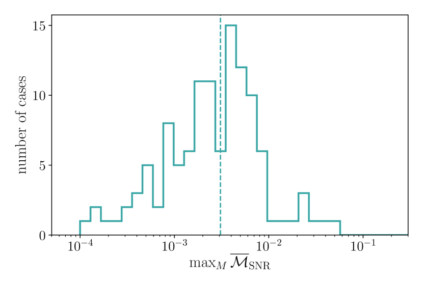
To assess the accuracy of the new NR waveforms, we compute the sky-and-polarization-averaged unfaithfulness defined in Eq. (10) between the highest and second highest resolutions in the NR simulation.
Figure 2 shows a histogram of the unfaithfulness, evaluated at maximized over the total mass, between 20 and 200 . It is apparent that the unfaithfulness is below for most cases, but there are several cases with much higher unfaithfulness. This tail to high unfaithfulness has been observed previously, when evaluating the accuracy of SXS simulations in Ref. Varma et al. (2019b). Therein, it was established that, when the non-astrophysical junk radiation perturbs the parameters of the simulation sufficiently, the different resolutions actually correspond to different physical systems. Thus, taking the difference between adjacent resolutions is no longer an appropriate estimate of the error.
We also find that the largest unfaithfulness occurs when the difference in parameters is largest, thus confirming that it is the difference in parameters that dominates the unfaithfulness.
II.4 Effect of mode asymmetries in numerical-relativity waveforms
The gravitational polarizations at time and location on the coordinate sphere from the binary can be decomposed in –spin-weighted spherical harmonics, as follows
| (14) |
For nonprecessing binaries, the invariance of the system under reflection across the orbital plane (taken to be the plane) implies . The latter is a very convenient relationship — for example it renders unnecessary to model modes with negative values of . However, this relationship is no longer satisfied for precessing binaries.
As investigated in previous NR studies Pekowsky et al. (2013); Boyle et al. (2014), we expect the asymmetries between opposite- modes to be small as compared to the dominant -mode emission (at least during the inspiral) in a co-rotating frame that maximizes emission in the modes, also known as the maximum-radiation frame Boyle et al. (2011); Boyle (2013). However, while the asymmetries are expected to be small during the inspiral, the difference in phase and amplitude between positive and negative -modes might become non-negligible at merger.
As we discuss in the next section, when building multipolar waveforms (SEOBNRv4PHM) for precessing binaries by rotating
modes from the co-precessing Buonanno et al. (2003); Schmidt et al. (2011); Boyle et al. (2011); O’Shaughnessy et al. (2011); Schmidt et al. (2012)
to the inertial frame of the observer, we shall neglect the mode asymmetries. To quantify the error introduced by this assumption,
we proceed as follows. We first take NR waveforms in the co-precessing frame and construct symmetrized waveforms. Specifically, we
consider the combination of waveforms in the co-precessing frame defined by (e.g., see Ref. Varma et al. (2019b))
| (15) |
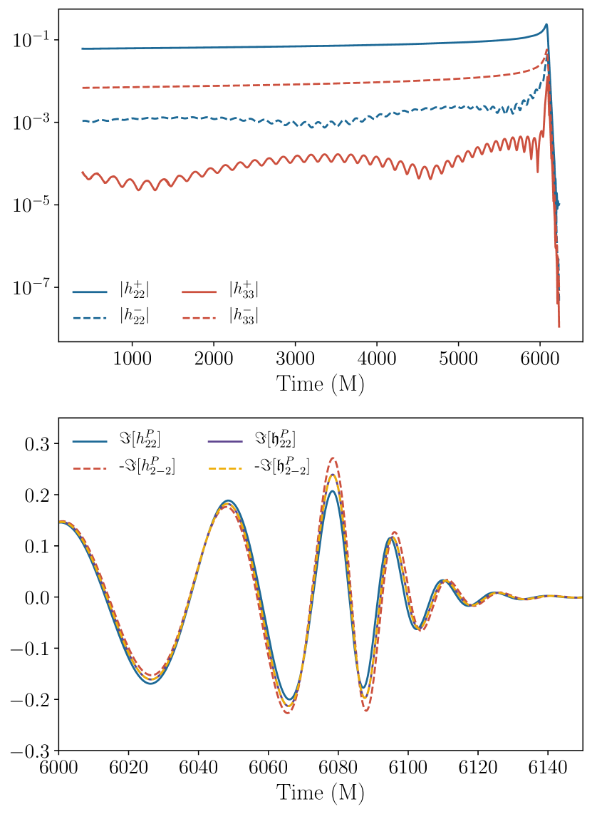
Note that if the assumption of conjugate symmetry holds (i.e., if ), then for even (odd) modes, () is non-zero while the other component vanishes. If the assumption does not hold, it is still true that at given , one of the components is much larger than the other, as shown in top panel of Fig. 3. Motivated by this, we define the symmetrized modes (for ) as Varma et al. (2019b)
| (16) |
The other modes are constructed as for ,
and we set modes to zero. The bottom panel of Fig. 3 shows an example
of asymmetrized waveform for the case PrecBBH000078 of the SXS catalogue, in the
co-precessing frame. It is obvious that the asymmetry between the
modes has been removed and that the symmetrized waveform does indeed
represent a reasonable “average” between the original modes. The symmetrized waveforms in the
inertial frame are obtained by rotating the co-precessing frames modes back to the inertial frame.
In Fig. 4, we show the sky-and-polarization averaged unfaithfulness between the NR waveforms and the symmetrized waveforms described above, maximized over the total mass, including all modes available in the NR simulation, that is up to . For the vast majority of the cases, the unfaithfulness is , and all cases have unfaithfulness below . This demonstrates that the effect of neglecting the asymmetry is likely subdominant to other sources of error such as the modeling of the waveform phasing, although the best way of quantifying the effect is to perform a Bayesian parameter-estimation study, which we leave to future work.
III Multipolar EOB waveforms for spinning, precessing binary black holes
We briefly review the main ideas and building blocks of the EOB approach, and then describe
an improved spinning, precessing EOBNR waveform model, which, for the first time, also contains
multipole moments beyond the quadrupolar one. The model is already
available in the LIGO Algorithm Library LAL under the name of SEOBNRv4PHM.
We refer the reader to Refs. Taracchini et al. (2012, 2014); Pan et al. (2014); Babak et al. (2017); Cotesta et al. (2018)
for more details of the EOB framework and its most recent waveform models.
Here we closely follow Ref. Babak et al. (2017), highlighting when needed differences with respect to the
previous precessing waveform model developed in Ref. Babak et al. (2017) (SEOBNRv3P 444We note that
whereas in LAL the name of this waveform approximant is SEOBNRv3, here we
add a “P” to indicate “precession”, making the notation uniform with respect to
the most recent developed model SEOBNRv4P Babak et al. (2017).).
III.1 Two-body dynamics
The EOB formalism Buonanno and Damour (1999, 2000); Damour et al. (2000); Damour (2001) can describe analytically the GW emission of the entire coalescence process, notably inspiral, merger and ringdown, and it can be made highly accurate by including information from NR. For the two-body conservative dynamics, the EOB approach relies on a Hamiltonian , which is constructed through: (i) the Hamiltonian of a spinning particle of mass and spin moving in an effective, deformed Kerr spacetime of mass and spin Barausse et al. (2009); Barausse and Buonanno (2010, 2011), and (ii) an energy map between and Buonanno and Damour (1999)
| (17) |
where is the symmetric mass ratio. The deformation of the effective Kerr metric is fixed by requiring that at any given PN order, the PN-expanded Hamiltonian agrees with the PN Hamiltonian for BBHs Blanchet (2014). In the EOB Hamiltonian used in this paper Barausse and Buonanno (2010, 2011), the spin-orbit (spin-spin) couplings are included up to 3.5PN (2PN) order Barausse and Buonanno (2010, 2011), while the non-spinning dynamics is incorporated through 4PN order Cotesta et al. (2018). The dynamical variables in the EOB model are the relative separation and its canonically conjugate momentum , and the spins . The conservative EOB dynamics is completely general and can naturally accommodate precession Pan et al. (2014); Babak et al. (2017) and eccentricity Hinderer and Babak (2017); Liu et al. (2020); Chiaramello and Nagar (2020).
When BH spins have generic orientations, both the orbital plane and the spins undergo precession about the total angular momentum of the binary, defined as , where . We also introduce the Newtonian orbital angular momentum , which at any instant of time is perpendicular to the binary’s orbital plane. Black-hole spin precession is described by the following equations
| (18) |
In the EOB approach, dissipative effects enter in the equations of motion through a nonconservative radiation-reaction force that is expressed in terms of the GW energy flux through the waveform multipole moments Buonanno et al. (2006); Damour and Nagar (2007); Damour et al. (2009); Pan et al. (2011) as
| (19) |
where is the (angular) orbital frequency, is the luminosity distance of the BBH to the observer, and the ’s are the GW multipole modes. As discussed in Refs. Cotesta et al. (2018); Bohé et al. (2017), the used in the energy flux are not the same as those used for building the gravitational polarizations in the inertial frame, since the latter include the nonquasi-circular corrections, which enforce that the SEOBNR waveforms at merger agree with the NR data, when available.
III.2 Inspiral-plunge waveforms
For the inspiral-plunge waveform, the EOB approach uses a factorized, resummed version Damour and Nagar (2007); Damour et al. (2009); Pan et al. (2011); Cotesta et al. (2018) of the frequency-domain PN formulas of the modes Arun et al. (2009); Mishra et al. (2016). As today, the factorized resummation has been developed only for quasicircular, nonprecessing BBHs Damour et al. (2009); Pan et al. (2011), and it has been shown to improve the accuracy of the PN expressions in the test-particle limit, where one can compare EOB predictions to numerical solutions of the Regge-Wheeler-Zerilli and Teukolsky equations Bernuzzi et al. (2011); Barausse et al. (2012); Taracchini et al. (2013); Harms et al. (2016).
The radiation-reaction force in Eq. (19) depends on the amplitude of the individual GW modes , which, in the non-precessing case, are functions of the constant aligned-spin magnitudes . In the precessing case, these modes depend on time, as , and they depend on the generic, precessing orbital dynamics through the radial separation and orbital frequency , which carry modulations due to spin-spin couplings whenever precession is present. However, we stress that with this choice of the radiation-reaction force and waveform model, not all spin-precession effects are included, since the PN formulas of the modes Arun et al. (2009) also contain terms that depend on the in-plane spin components.
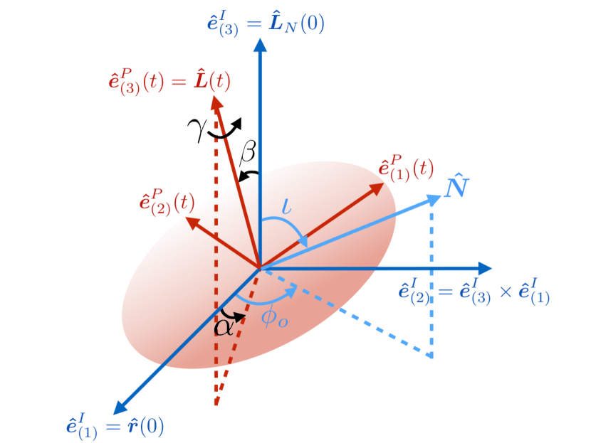
For data-analysis purposes, we need to compute the GW polarizations in the inertial-frame of the observer (or simply observer’s frame). We denote quantities in this frame with the superscript . The observer’s frame is defined by the triad (), where , and . Moreover, in this frame, the line of sight of the observer is parametrized as (see Fig. 5). We also introduce the observer’s frame with the polarization basis such that and , which spans the plane orthogonal to .
To compute the observer’s-frame modes during the inspiral-plunge stage, it is convenient to introduce a non-inertial reference frame that tracks the motion of the orbital plane, the so-called co-precessing frame (superscript ), described by the triad (). At each instant, its -axis is aligned with : 555Note that in Ref. Babak et al. (2017), the -axis is aligned with instead of .. In this frame, the BBH is viewed face-on at all times, and the GW radiation looks very much nonprecessing Buonanno et al. (2003); Schmidt et al. (2011); Boyle et al. (2011); O’Shaughnessy et al. (2011); Schmidt et al. (2012). The other two axes lie in the orbital plane and are defined such as they minimize precessional effects in the precessing-frame modes Buonanno et al. (2003); Boyle et al. (2011). After introducing the vector , we enforce the minimum-rotation condition by requiring that and (see also Fig. 5). As usual, we parametrize the rotation from the precessing to the observer’s frame through time-dependent Euler angles , which we compute using Eqs. (A4)–(A6) in Appendix A of Ref. Babak et al. (2017). We notice that the minimum-rotation condition can also be expressed through the following differential equation for : with .
We compute the precessing-frame inspiral-plunge modes just like we do for the GW flux, namely by evaluating the factorized, resummed nonprecessing multipolar waveforms along the EOB precessing dynamics, and employing the time-dependent spin projections . Finally, the observer’s-frame inspiral-plunge modes are obtained by rotating the precessing-frame inspiral-plunge modes using Eq. (A13) in Appendix A of Ref. Babak et al. (2017).
Following Ref. Cotesta et al. (2018), where an EOBNR
nonprecessing multipolar waveform model was developed (SEOBNRv4HM),
here we include in the precessing frame of the SEOBNRv4PHM model the
and modes,
and make the assumption . As shown in Sec. II.4, we expect that inaccuracies
due to neglecting mode asymmetries should remain mild, or at most at the level of other modeling errors.
III.3 Merger-ringdown waveforms
The description of a BBH as a system composed of two individual objects is of course valid only up to the merger. After that point, the EOB model builds the GW emission (ringdown stage) via a phenomenological model of the quasinormal modes (QNMs) of the remnant BH, which forms after the coalescence of the progenitors. The QNM frequencies and decay times are known (tabulated) functions of the mass and spin of the remnant BH Berti et al. (2006). Since the QNMs are defined with respect to the direction of the final spin, the specific form of the ringdown signal, as a linear combination of QNMs, is formally valid only in an inertial frame whose -axis is parallel to .
A novel feature of the SEOBNRv4PHM waveform model presented here is that we attach
the merger-ringdown waveform (notably each multipole mode )
directly in the co-precessing frame, instead of the observer’s frame. As a consequence,
we can employ here the merger-ringdown multipolar model developed for non-precessing BBHs
(SEOBNRv4HM) in Ref. Cotesta et al. (2018) (see Sec. IVE therein for details).
By contrast, in the SEOBNRv3P waveform model Babak et al. (2017), the
merger-ringdown waveform was built as a superposition of
QNMs in an inertial frame aligned with the direction of the remnant spin.
This construction was both more complicated to implement and more prone to numerical
instabilities.
To compute the waveform in the observer’s frame, our approach requires a description of the co-precessing frame Euler angles that extends beyond the merger. To prescribe this, we take advantage of insights from NR simulations O’Shaughnessy et al. (2013). In particular, it was shown that the co-precessing frame continues to precess roughly around the direction of the final spin with a precession frequency approximately equal to the differences between the lowest overtone of the (2,2) and (2,1) QNM frequencies, while the opening angle of the precession cone decreases somewhat at merger. We find that this behavior is qualitatively correct for the NR waveforms used for comparison in this paper.
To keep our model generic for a wide range of mass ratios and spins, we need an extension of the behavior noticed in Ref. O’Shaughnessy et al. (2013) to the retrograde case, where the remnant spin is negatively aligned with the orbital angular momentum at merger. Such configurations can occur for high mass-ratio binaries, when the total angular momentum is dominated by the spin of the primary instead of the orbital angular momentum . This regime is not well explored by NR simulations, and includes in particular systems presenting transitional precession Apostolatos et al. (1994). In our model we keep imposing simple precession around the direction of the remnant spin at a rate , but we distinguish two cases depending on the direction of the final spin (approximated by the total angular momentum at merger) relative to the final orbital angular momentum :
| (20) |
where , and the zero-overtone QNM frequencies for negative are taken on the branch that continuously extends the , branch Berti et al. (2006) (the QNM refers to zero overtone). In both cases, . We do not attempt to model the closing of the opening angle of the precession cone and simply consider it to be constant during the post-merger phase, . The third Euler angle is then constructed from the minimal rotation condition . The integration constants are determined by matching with the inspiral at merger. We find that the behavior of Eq. (20) in the case is qualitatively consistent with an NR simulation investigated by one of us Ossokine (2020). However, we stress that this prescription for the retrograde case is much less tested than for the prograde case.
Furthermore, one crucial aspect of the above construction is the mapping from the
binary’s component masses and spins to the final mass and spin, which is
needed to compute the QNM frequencies of the merger remnant. Many groups have developed fitting formulae based
on a large number of NR simulations (e.g., see Ref. Varma et al. (2019c) for an overview).
To improve the agreement of our EOB merger-ringdown model with NR, and to ensure agreement
in the aligned-spin limit with SEOBNRv4 Bohé et al. (2017) and SEOBNRv4HM Cotesta et al. (2018),
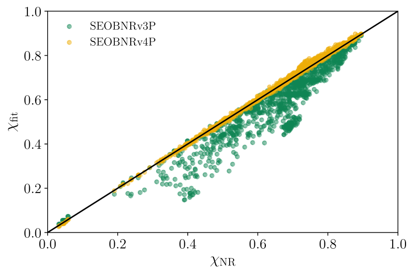
we employ the fits from Hofmann et al. Hofmann et al. (2016). In Fig. 6 we compare
the performance of the fit used in the previous EOB precessing model SEOBNRv3P Pan et al. (2014); Taracchini et al. (2014); Babak et al. (2017) to the fit from Hofmann et al. that we adopt for SEOBNRv4PHM. It is clear that the new fit reproduces NR
data much better. This in turn improves the correspondence between NR and EOB QNM frequencies.
For the final mass we employ the same fit as in previous EOB models, and we provide it here since it was not given explicitly anywhere before:
| (21) | |||||
where , and is the binding energy of the Kerr spacetime at the innermost stable circular orbit Bardeen et al. (1972).
Finally, for precessing binaries, the individual components of the spins vary with time. Therefore, in applying the fitting formulae to obtain final mass and spin, one must make a crucial choice in selecting the time during the inspiral stage at which the spin directions are evaluated. In fact, even if one considers a given physical configuration, evaluating the final spin formulae with spin directions from different times yields different final spins and consequently different waveforms. We choose to evaluate the spins at a time corresponding to the separation of . This choice is guided by two considerations: by the empirical finding of good agreement with NR (e.g., performing better than using the time at which the inspiral-plunge waveform is attached to the merger-ringdown waveform Cotesta et al. (2018)), and by the restriction that the waveform must start at in order to have small initial eccentricity Babak et al. (2017). Thus, our choice ensures that a given physical configuration always produces the same waveform regardless of the initial starting frequency.
To obtain the inspiral-merger-ringdown modes in the inertial frame, , we rotate the inspiral-merger-ringdown modes from the co-precessing frame to the observer’s frame using the rotation formulas and Euler angles in Appendix A of Ref. Babak et al. (2017). The inertial frame polarizations then read
| (22) |
III.4 On the fits of calibration parameters in presence of precession
The SEOBNRv4PHM waveform model inherits the EOB Hamiltonian and GW energy flux from the aligned-spin model
SEOBNRv4 Bohé et al. (2017), which features higher (yet unknown) PN-order terms in the dynamics
calibrated to NR waveforms. These calibration parameters were denoted and in Ref. Bohé et al. (2017),
and were fitted to NR and Teukolsky-equation–based waveforms
as polynomials in where ) with
the spin of the EOB background
spacetime. In contrast to the SEOBNRv3P waveform model, which used the EOB Hamiltonian and GW energy flux
from the aligned-spin model SEOBNRv2Taracchini et al. (2014), the fits in
Ref. Bohé et al. (2017) include odd powers of and thus the sign of matters
when the BHs precess.
The most natural way to generalize these fits to the precessing case is to project onto the orbital angular momentum in the usual spirit of reducing precessing quantities to corresponding aligned-spin ones. To test the impact of this prescription, we compute the sky-and-polarization-averaged unfaithfulness with the set of 118 NR simulations described in Sec. II, and find that while the majority of the cases have low unfaithfulness (%), there are a handful of cases where it is significant(%), with many of them having large in-plane spins.
To eliminate the high mismatches, we introduce the augmented spin that includes contribution of the in-plane spins:
| (23) |
Here and is a positive coefficient to be determined. Note that the extra term in the definition of the augmented spin for any combination of the spins. We set when . Fixing insures that the augmented spin obeys the Kerr bound. Using the augmented spin eliminates all mismatches above , and thus greatly improves the agreement of the model with NR data.
IV Comparison of multipolar precessing models to numerical-relativity waveforms
To assess the impact of the improvements incorporated in the SEOBNRv4PHM waveform model, we compare this model and other models publicly available
in LAL (see Table 1) to the set of simulations described in Sec. II, as well as to all publicly available precessing SpEC simulations 666The list of all
SXS simulations used can be found in https://arxiv.org/src/1904.04831v2/anc/sxs_catalog.json.
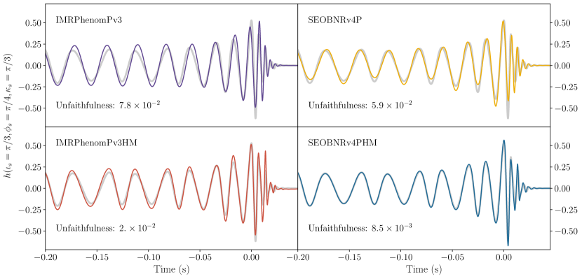
We start by comparing in Fig. 7, the precessing NR
waveform PrecBBH00078 with mass ratio , BH’s spin magnitudes , total mass
and modes from the new 118 SXS catalog (see Appendix B) to the precessing waveforms IMRPhenomPv3 and SEOBNRv4P with modes (upper panels), and to
the precessing multipolar waveforms IMRPhenomPv3HM and SEOBNRv4PHM
(lower panels). This NR waveform is the most “extreme” configuration from the
new set of waveforms and has about 44 GW cycles before merger, and the plot only shows
the last cycles. More specifically, we plot the detector
response function given in Eq. (II.2), but we leave out the overall constant amplitude.
We indicate on the panels the unfaithfulness for the different cases. We note the improvement when including modes beyond the quadrupole.
SEOBNRv4PHM agrees particularly well to this NR waveform, reproducing accurately the higher-mode features throughout merger and ringdown.
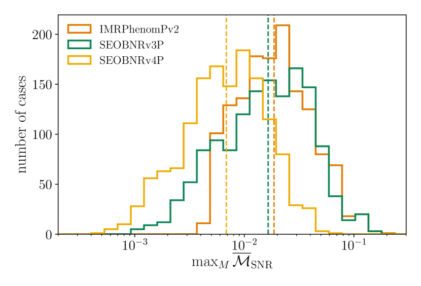
We now turn to the public precessing SXS NR catalog of 1404 waveforms. First, to quantify the performance of the new precessing waveform model SEOBNRv4P
with respect to previous precessing models used in LIGO and Virgo inference studies, we compute the unfaithfulness 777We always use the sky-and-polarization averaged, SNR-weighted faithfulness or
unfaithfulness unless otherwise stated. against the precessing NR catalog, including only the dominant
multipoles in the co-precessing frame. Figure 8 shows the histograms of the largest
mismatches when the binary total mass varies in the range . Here, we also consider the
precessing waveform models used in the first GW Transient Catalog Abbott et al. (2019) of the
LIGO and Virgo collaboration (i.e., SEOBNRv3P and IMRPhenomPv2).
Two trends are apparent: firstly, SEOBNRv3P and IMRPhenomPv2 distributions are
broadly consistent, with both models having mismatches which extend beyond , although SEOBNRv3 has more cases at lower unfaithfulness; secondly, SEOBNRv4P
has a distribution which is shifted to much lower values of the unfaithfulness and does not include outliers with the largest
unfaithfulness below .
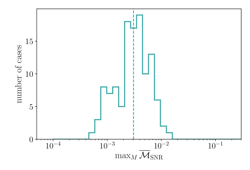
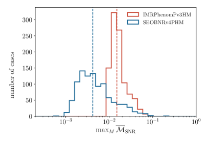
Next, we examine the importance of higher modes. To do so, we use SEOBNRv4PHM
with and without the higher modes, while always including all modes up to
in the NR waveforms. As can be seen in Fig. 9,
if higher modes are omitted, the unfaithfulness can be very large, with a
significant number of cases having unfaithfulness , as has been seen in many past studies.
On the other hand, once higher modes are included in the model, the distribution of mismatches becomes
much narrower, with all mismatches below . Furthermore, the distribution now
closely resembles the distribution of mismatches when only modes were
included in the NR waveforms. Thus, we see that higher modes play an important role
and are accurately captured by SEOBNRv4PHM waveform model.
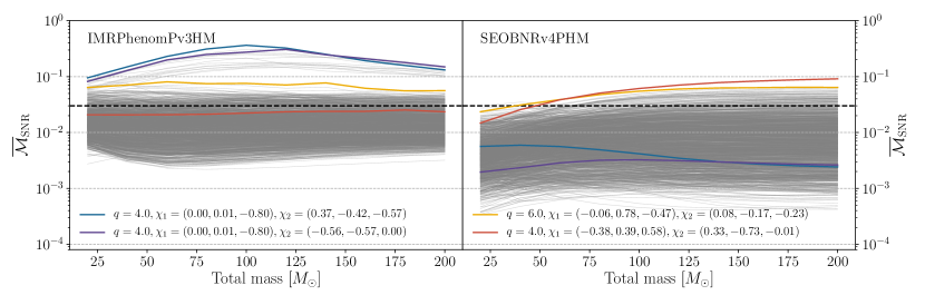
Moreover, in Fig. 10 we display, for a specific choice of the inclination, the
unfaithfulness versus the binary’s total mass between the public precessing SXS NR catalog and
SEOBNRv4PHM and IMRPhenomPv3HM. We highlight with curves in color the NR configurations having worst maximum
mismatches for the two classes of approximants. For the majority of cases, both models have unfaithfulness below 5%, but
SEOBNRv4PHM has no outliers beyond 10% and many more cases at lower unfaithfulness (). We find that
the large values of unfaithfulness above for IMRPhenomPv3HM come from simulations with and large anti-aligned primary spin,
i.e. . An examination of the waveforms in this region reveals that unphysical features develop
in the waveforms, with unusual oscillations both in amplitude and phase. For lower spin magnitudes these features are milder, and disappear
for spin magnitudes . These features are present also in IMRPhenomPv3 and are thus connected to the
precession dynamics, a region already known to potentially pose a challenge when modeling the
precession dynamics as suggested in Ref. Chatziioannou et al. (2017), and adopted in Ref. Khan et al. (2020).
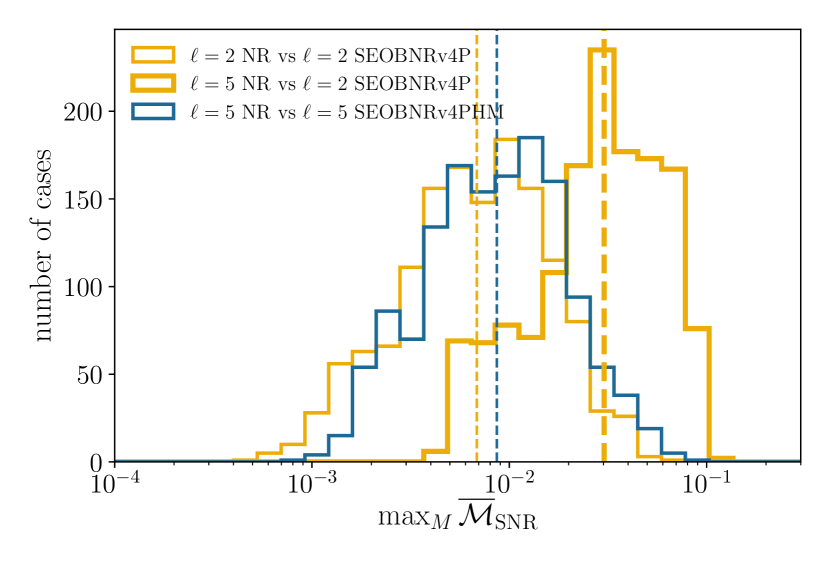
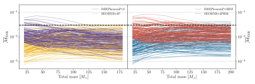
We now focus on the comparisons with the 118 SXS NR waveforms produced
in this paper. In Fig. 11 we show the
unfaithfulness for IMRPhenomPv3(HM) and SEOBNRv4P(HM) in
the left (right) panels. We compare waveforms without higher modes, to
NR data that has only the modes, and the other models to NR
data with modes. The performance of both waveform models
on this new NR data set is largely comparable to what was found for
the public catalog. Both families perform well on average, with most
cases having unfaithfulness below 2% for models without higher modes
and 3% for models with higher modes. However, for some configurations
IMRPhenomPv3(HM) reaches unfaithfulness values above for
total masses below . Once again, the overall
distribution is shifted to lower unfaithfulness values for
SEOBNRv4P(HM).
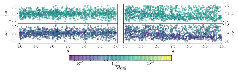
When studying the distribution of unfaithfulness for these 118 cases across parameter space, it is useful to introduce the widely used effective Damour (2001); Racine (2008); Santamaria et al. (2010) and precessing Schmidt et al. (2015) spins. These capture the leading order aligned-spin and precession effects respectively, and are defined as
| (24a) | ||||
| (24b) | ||||
where with , and we indicate with the projection of the spins on the orbital plane. We find that the unfaithfulness shows 2 general trends. First, it tends to increase with increasing and . Secondly, that cases with positive (i.e. aligned with Newtonian orbital angular momentum) tend to have larger unfaithfulness. This is likely driven by the fact that inspiral is longer for such cases and the binary merges at higher frequency. We do not find any other significant trends based on spin directions. It is interesting to note that the distribution of mismatches from the 118 cases is quite similar to the distribution from the much larger public catalog. This suggests that the 118 cases do indeed explore many different regimes of precession.
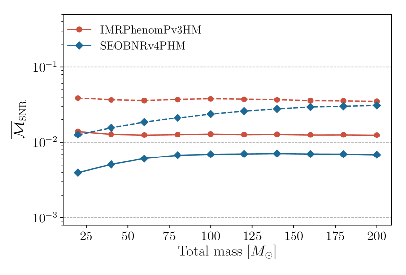
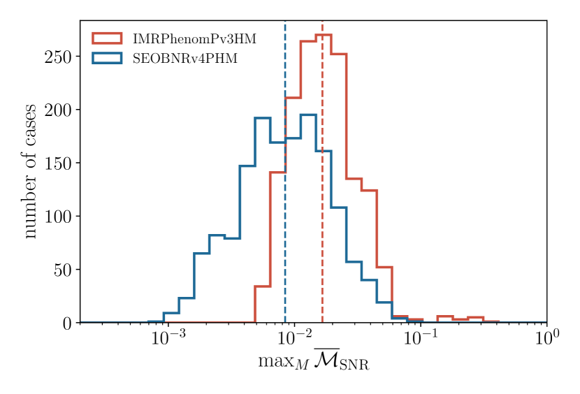
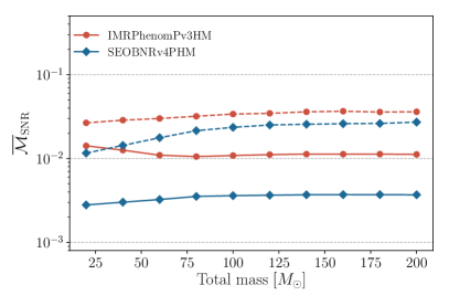
To further quantify the results of the comparison between the precessing multipolar models SEOBNRv4PHM and IMRPhenomPv3HM and
the NR waveforms, we show in Figs. 12 and 13 the median and -percentile of all cases,
and the highest unfaithfulness as function of the total mass, respectively. These studies also demonstrate the better performance of
SEOBNRv4PHM with respect to IMRPhenomPv3HM.
To summarize the performance against the entire SXS catalog (including the new 118 precessing waveforms) we find that
for SEOBNRv4PHM, out of a total of 1523 NR simulations we have considered, 864 cases ( ) have a maximum unfaithfulness less than ,
and 1435 cases ( ) have unfaithfulness less than . Meanwhile for IMRPhenomPv3HM the numbers become 300 cases ( ) below , 1256 cases
( ) below 888Due to technical details of the IMRPhenomPv3HM model, the total number of cases analyzed for this model is 1507 instead of 1523..
The accuracy of the semi-analytical waveform models can be improved in the future by calibrating them to the precession sector of the SXS NR waveforms.
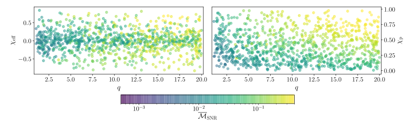
An interesting question is to examine the behavior of the precessing models outside the region in which their underlying aligned-spin waveforms were calibrated. To this effect we consider 1000 random cases
between mass ratios and spin magnitudes and compute between
SEOBNRv4PHM and IMRPhenomPv3HM. Figure 14 shows the dependence of the unfaithfulness on the binary parameters,
in particular the mass ratio, and the effective and precessing spins. We find that for mass ratios , of cases have unfaithfulness below 2% and 90%
have unfaithfulness below 10%. The unfaithfulness grows very fast with mass ratio and spin, with the highest unfaithfulness occurring at the highest mass ratio and
precessing spin. This effect is enhanced due to the fact that we choose to start all the waveforms at the same frequency and for higher mass ratios, the number of cycles in
band grows as where is the symmetric mass ratio. These results demonstrate the importance of producing long NR simulations for large mass ratios
and spins, which can be used to validate waveform models in this more extreme region of the parameter space. To design more accurate semi-analytical models
in this particular region, it will be relevant to incorporate in the models the information from gravitational self-force Damour (2010); Bini et al. (2018); Antonelli et al. (2020),
and also test how the choice of the underlying EOB Hamiltonians with spin effects Rettegno et al. (2019); Khalil et al. (2020) affects the accuracy.
Finally, in Appendix A we quantify the agreement of the precessing multipolar waveform models
SEOBNRv4PHM and IMRPhenomPv3HM against the NR surrogate model NRSur7dq4 Varma et al. (2019b), which
was built for binaries with mass ratios , BH’s spins up to and binary’s
total masses larger than . We find that the unfaithfulness between the semi-analytic models and the NR surrogate largely mirrors the results of the
comparison in Figs. 12 and 13. Notably, as it can be seen in Fig. 17, the unfaithfulness is generally below 3% for both waveform
families, but SEOBNRv4PHM outperforms IMRPhenomPv3HM with the former having a median at , while the latter is at .
V Bayesian analysis with multipolar precessing waveform models
We now study how the accuracy of the waveform model SEOBNRv4PHM (and also IMRPhenomPv3HM), which we have
quantified in the previous section through the unfaithfulness, affects parameter inference when synthetic signal injections are performed.
To this end, we employ two mock BBH signals and do not add any detector noise to them
(i.e., we work in zero noise), which is equivalent to average over many different noise realizations. This choice avoids
arbitrary biases introduced by a random-noise realization, and it is reasonable
since the purpose of this analysis is to estimate possible biases in the
binary’s parameters due to inaccuracies in waveform models.
We generate the first precessing-BBH mock signal with the
NRSur7dq4 model. It has mass ratio and a total
source-frame mass of . The spins of the two BHs are
defined at a frequency of Hz, and have components and . The masses and
spins” magnitudes ( and ) of this injection are compatible
with those of BBH systems observed so far with LIGO and Virgo
detectors Abbott
et al. (2016b); Abbott et al. (2019); Zackay et al. (2019); Venumadhav et al. (2019); Nitz et al. (2019).
Although the binary’s parameters are not extreme, we choose the
inclination with respect to the line of sight of the BBH to be
, to emphasize the effect of higher
modes. The coalescence and polarization phase, respectively and
, are chosen to be 1.2 rad and 0.7 rad. The sky-position is
defined by its right ascension of 0.33 rad and its declination of -0.6
rad at a GPS-time of 1249852257 s. Finally, the distance to the source
is set by requesting a network-SNR of in the three detectors
(LIGO Hanford, LIGO Livingston and Virgo) when using the Advanced LIGO
and Advanced Virgo PSD at design sensitivity Barsotti et al. (2018). The
resulting distance is Mpc. The unfaithfulness against this
injection is and for SEOBNRv4PHM and
IMRPhenomPv3HM, respectively. Although the value of
the network-SNR is large for this synthetic signal, it is not
excluded that the Advanced LIGO and Virgo detectors at design
sensitivity could detect such loud BBH. With this study we
want to test how our waveform model performs on a system with moderate
precessional effect when detected with a large SNR value,
considering that it has an unfaithfulness of .
For the second precessing-BBH mock signal, we use a binary with larger mass ratio
and spin magnitude for the primary BH. We employ the NR waveform SXS:BBH:0165 from
the public SXS catalog having mass ratio , and we choose the source-frame total mass
. The BH’s spins, defined at a frequency of Hz, have values
and . The BBH system in this simulation has strong
spin-precession effects. We highlight that this NR waveform is one of the worst cases in term of unfaithfulness
against SEOBNRv4PHM, as it is clear from Fig. 10.
For this injection we choose the binary’s inclination to be
edge-on at Hz to strongly emphasize higher modes. All
the other binary parameters are the same of the previous injection,
with the exception of the luminosity distance, which
in this case is set to be Gpc to obtain a
network-SNR of . The NR waveform used for
this mock signal has unfaithfulness of for SEOBNRv4PHM and for IMRPhenomPv3HM,
thus higher than in the first injection.
For the parameter-estimation study we use the software PyCBC’s pycbc_generate_hwinj Nitz et al. (2020) to prepare the mock signals, and we perform the Bayesian analysis with parallel Bilby Smith and Ashton (2019), a highly parallelized version of the parameter-estimation software Bilby Ashton et al. (2019). We choose a uniform prior in component masses in the range . Priors on the dimensionless spin magnitudes are uniform in , while for the spin directions we use prior isotropically distributed on the unit sphere. The priors on the other parameters are the standard ones described in Appendix C.1 of Ref. Abbott et al. (2019).
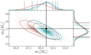
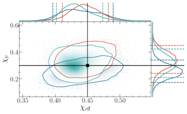
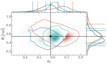
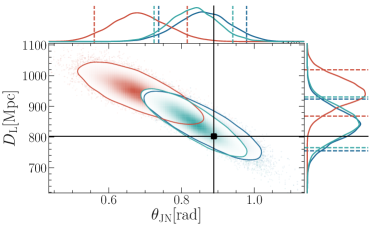

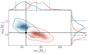
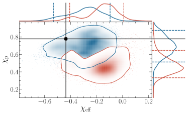
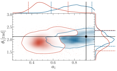
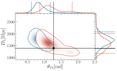
We summarize in Fig. 15 the results of the parameter
estimation for the first mock signal for SEOBNRv4PHM (blue),
IMRPhenomPv3HM (red) and NRSur7dq4 (cyan). We report
the marginalized 2D and 1D posteriors for the component masses
and in the source frame (top left), the effective spin
parameters and (top right),
the spin magnitude of the more massive BH and its tilt angle
(bottom left) and finally the angle
and the luminosity distance (bottom right). In the 2D posteriors, solid
contours represent credible intervals and black dots show the
value of the parameter used in the synthetic signal. In the 1D
posteriors, they are represented respectively by dashed lines and black
solid lines. As it is clear from Fig. 15, when using the
waveform models SEOBNRv4PHM and NRSur7dq4, all the
parameters of the synthetic signal are correctly measured within the
statistical uncertainty. Moreover, the shape of the posterior
distributions obtained when using SEOBNRv4PHM are similar to
those recovered with NRSur7dq4 (the model used to create the
synthetic signal). This means that the systematic error due to a non
perfect modeling of the waveforms is negligible in this case.
For the model IMRPhenomPv3HM while masses and spins
are correctly measured within the statistical uncertainty, the
luminosity distance and the angle are
biased. This is consistent with the prediction obtained using
Lindblom’s criterion in Refs. Flanagan and Hughes (1998); Lindblom et al. (2008); McWilliams et al. (2010); Chatziioannou et al. (2017) 999The
criterion says that a sufficient, but not necessary condition for
two waveforms to become distinguishable is that the unfaithfulness , where is the
number of binary’s intrinsic parameters, which we take to be 8 for a
precessing-BBH system. Note, however, that in practice this factor
can be much larger, see discussion in
Ref. Pürrer and Haster (2019).. In fact, according to this criterion,
an unfaithfulness of for IMRPhenomPv3HM would be
sufficient to produce biased results at a network-SNR of . Thus,
it is expected to observe biases when using IMRPhenomPv3HM at
the network-SNR of the injection, which is . In the case of
SEOBNRv4PHM the unfaithfulness against the signal waveform is
and according to Lindblom’s criterion we should also expect
biases for network-SNRs larger than , but in practice we do not
observe them. We remind that Lindblom’s criterion is only approximate
and it has been shown in Ref. Pürrer and Haster (2019) to be too
conservative, therefore the lack of bias that we observe is not
surprising.

In Fig. 16 we summarize the results of
the second mock-signal injection. The plots are the same as in Fig. 15
with the only exception that we do not have results for the NRSur7dq4
model since it is not available in this region of the parameter space. In
this case the unfaithfulness between SEOBNRv4PHM
(IMRPhenomPv3HM) and the NR waveform used for the mock signal
is (). According to Lindblom’s criterion, at the
network-SNR of this mock signal we should expect the bias due to
non-perfect waveform modeling to be dominant over the statistical
uncertainty for an unfaithfulness . Therefore we might expect some biases in inferring parameters
for both models. Lindblom’s criterion does not say which parameters
are biased and by how much. The results in Fig. 16 clearly show
that both models have biases in the measurement of some
parameters, but unfaithfulness of and induce different
amount of biases and also on different set of parameters (intrinsic and extrinsic).
In particular for the component masses (top left panel of
Fig. 16), the 2D posterior distribution obtained with
SEOBNRv4PHM barely include the value used for the mock signal
in the credible region. This measurement looks better when
focusing on the 1D posterior distributions for the individual masses
for which the injection values are well within the credible intervals.
The situation is worst for the IMRPhenomPv3HM model, for which the 2D posterior
distribution barely excludes the injection value at
credible level. In this case also the true value of
is excluded from the credible interval of the marginalized 1D
posterior distribution. Furthermore, and (top right
panel of Fig. 16) are correctly measured with
SEOBNRv4PHM while the measurement with IMRPhenomPv3HM
excludes the true value from the 2D credible region. From the
1D posterior distributions it is clear that the source of this inaccuracy
is the incorrect measurement of , while
is correctly recovered within the credible interval. A similar
situation is observed in the measurement of the spin magnitude
of the heavier BH and its tilt angle (bottom left panel of
Fig. 16). Also in this case SEOBNRv4PHM correctly
measures the parameters used in the mock signal, while
IMRPhenomPv3HM yields an incorrect measurement due to a bias in
the estimation of . Finally, we focus on the measurement of the
angle and the luminosity distance (bottom left
panel of Fig. 16). In this case the value of these
parameters used in the synthetic signal is just slightly measured
within the credible region of the 2D posterior distribution
obtained with SEOBNRv4PHM. As a consequence the luminosity
distance is also barely measured within the credible interval
from the marginalized 1D posterior distribution and the measured value
of results outside the credible interval of
the 1D posterior distribution. The posterior distributions obtained
using IMRPhenomPv3HM are instead correctly measuring the
parameters of the mock signal. We can conclude that even with an
unfaithfulness of against the NR waveform used for the mock
signal the SEOBNRv4PHM model is able to correctly measure most
of the binary parameters, notably the intrinsic ones, such as masses
and spins.
VI Conclusions
In this paper we have developed and validated the first inspiral-merger-ringdown precessing
waveform model in the EOB approach, SEOBNRv4PHM, that includes multipoles beyond the dominant quadrupole.
Following previous precessing SEOBNR models Pan et al. (2014); Taracchini et al. (2014); Babak et al. (2017),
we have built such a model twisting up the aligned-spin waveforms of SEOBNRv4HM Bohé et al. (2017); Cotesta et al. (2018)
from the co-precessing Buonanno et al. (2003); Schmidt et al. (2011); Boyle et al. (2011); O’Shaughnessy et al. (2011); Schmidt et al. (2012)
to the inertial frame, through the EOB equations of motion for the spins and orbital angular momentum.
With respect to the previous precessing SEOBNR model, SEOBNRv3P Babak et al. (2017),
which has been used in LIGO/Virgo data analysis Abbott et al. (2016c, 2017d, 2019), the new model
(i) employs a more accurate aligned-spin two-body dynamics, since, in the non-precessing limit, it reduces to
SEOBNRv4HM, which was calibrated to 157 SXS NR simulations Mroue et al. (2013); Chu et al. (2016), and 13 waveforms Barausse et al. (2012)
from BH perturbation theory, (ii) includes in the co-precessing frame the modes
and , instead of only , (iii) incorporates the merger-ringdown
signal in the co-precessing frame instead of the inertial frame, (iv) describes the merger-ringdown stage through a phenomenological
fit to NR waveforms Bohé et al. (2017); Cotesta et al. (2018), and (v) uses more accurate NR fits for the final spin of the remnant BH.
The improvement in accuracy between SEOBNRv4 and SEOBNRv3P (i.e., the models with only the modes)
is evident from Fig. 8, where we have compared those models to the public SXS catalog of 1405 precessing
NR waveforms, and the new 118 SXS NR waveforms produced for this work. The impact of including higher modes in semi-analytical models to achieve higher accuracy to multipolar NR waveforms is demonstrated in Fig. 9. Figures 10, 11, 12 and 14 quantify the comparison of the
multipolar precessing SEOBNRv4PHM and IMRPhenomPv3HM to all SXS NR precessing waveforms at our disposal. We have found that for the SEOBNRv4PHM model, ( ) of the cases have maximum unfaithfulness value, in the
total mass range , below (). Those numbers change to ( ) when using the IMRPhenomPv3HM. The better accuracy of
SEOBNRv4PHM with respect to IMRPhenomPv3HM is also confirmed by
the comparisons with the NR surrogate model NRSur7dq4, as shown in Fig. 17. We have investigated
in which region of the parameter space the unfaithfulness against NR waveforms and NRSur7dq4 lies, and have found, not surprisingly,
that it occurs where both mass ratios and spins are large (see Fig. 18). When comparing SEOBNRv4PHM and IMRPhenomPv3HM outside
the region in which their corresponding aligned-spin underlying models were calibrated, we have also found that the largest differences reside when mass ratios are larger than 4 and spins
larger than 0.8 (see Fig. 14).
To improve the accuracy of the models in those more challenging regions, we would need NR simulations, but also more information from analytical
methods, such as the gravitational self-force Damour (2010); Bini et al. (2018); Antonelli et al. (2020), and resummed EOB Hamiltonians
with spins Rettegno et al. (2019); Khalil et al. (2020).
To quantify how the modeling inaccuracy, estimated by the unfaithfulness, impacts the inference of binary’s parameters, we have perfomed two parameter-estimation studies using Bayesian analysis. Working with the Advanced LIGO and Virgo network at design sensitivity, we have injected in zero noise two precessing-BBH mock signals with mass ratio 3 and 6, having SNR of 50 and 21, with inclination of and with respect to the line of sight respectively, and recovered them with SEOBNRv4PHM and IMRPhenomPv3HM. The unfaithfulness values of those models against the synthetic signals considered (i.e., NRSurd7q4 and SXS:BBH:0165) range from to . The results are summarized in Figs. 15 and 16. Overall, we have found that Lindblom’s criterion Flanagan and Hughes (1998); Lindblom et al. (2008); McWilliams et al. (2010); Chatziioannou et al. (2017); Pürrer and Haster (2019) is too conservative and predicts visible biases at SNRs lower than what we have obtained through the Bayesian analysis. In particular, we have found, when doing inference with SEOBNRv4PHM, that an unfaithfulness of may produce no biases up to SNR of 50, while an unfaithfulness of can produce biases only for some extrinsic parameters, such as distance and inclination, but not for binary’s masses and spins at SNR of 21. A more comprehensive Bayesian study will be needed to quantify, in a more realistic manner, the modeling systematics of SEOBNRv4PHM, if this model were used during the fourth observation run of Avanced LIGO and Virgo in 2022 (i.e., the run at design sensitivity).
The improvement in accuracy between SEOBNRv4 and
SEOBNRv3P (i.e., the models with only the modes) is
evident from Fig. 8, where we have
compared those models to the public SXS catalog of 1405 precessing NR
waveforms, and the new 118 SXS NR waveforms produced for this
work. The impact of including higher modes in semi-analytical models
to achieve higher accuracy to multipolar NR waveforms is demonstrated
in
Fig. 9. Figures 10,
11, 12 and
14 quantify the comparison of the multipolar
precessing SEOBNRv4PHM and IMRPhenomPv3HM to all SXS NR
precessing waveforms at our disposal. We have found that for the
SEOBNRv4PHM model, ( ) of the cases have
maximum unfaithfulness value, in the total mass range
, below (). Those numbers change to
( ) when using the
IMRPhenomPv3HM. We have found several cases with large
unfaithfulness () for IMRPhenomPv3HM, coming from a
region of parameter space with and large ()
spins anti-aligned with the orbital angular momentum, which
appear to be connected to unphysical features in the underlying
precession model, and cause unusual oscillations in the
waveform’s amplitude and phase. The better accuracy of SEOBNRv4PHM with
respect to IMRPhenomPv3HM is also confirmed by the comparisons
with the NR surrogate model NRSur7dq4, as shown in
Fig. 17. We have investigated in which region
of the parameter space the unfaithfulness against NR waveforms and
NRSur7dq4 lies, and have found, not surprisingly, that it occurs
where both mass ratios and spins are large (see
Fig. 18). When comparing SEOBNRv4PHM
and IMRPhenomPv3HM outside the region in which the aligned-spin
underlying model was calibrated, we have also found that the largest
differences reside when mass ratios are larger than 4 and spins larger
than 0.8 (see Fig. 14). To improve the accuracy
of the models in those more challenging regions, we would need NR
simulations, but also more information from analytical methods, such
as the gravitational
self-force Damour (2010); Bini et al. (2018); Antonelli et al. (2020), and
resummed EOB Hamiltonians with
spins Rettegno et al. (2019); Khalil et al. (2020).
The newly produced 118 SXS NR waveforms extend the coverage of binary’s parameter space, spanning
mass ratios , (dimensionless) spins , and different orientations
to maximize the number of precessional cycles. As we have emphasized, the waveform model SEOBNRv4HM
is not calibrated to NR waveforms in the precessing sector, only the aligned-spin sector was calibrated
in Refs. Bohé et al. (2017); Cotesta et al. (2018). Despite this,
the accuracy of the model is very good, and it can be further improved in the future if we calibrate
the model to the plus SXS NR precessing waveforms at our disposal. This will be an important
goal for the upcoming LIGO and Virgo O4 run in early 2022. Furthermore, SEOBNRv4HM assumes the following
symmetry among modes in the co-precessing frame, which however
no longer holds in presence of precession. As discussed in Sec. II.4, forcing
this assumption causes unfaithfulness on the order of a few percent. Thus, to achieve better accuracy,
when calibrating the model to NR waveforms, the mode-symmetry would need to be relaxed.
Finally, SEOBNRv4HM uses PN-resumed factorized modes that were developed for aligned-spin BBHs Damour et al. (2009); Pan et al. (2011),
thus they neglect the projection of the spins on the orbital plane. To obtain high-precision waveform models, it will
be relevant to extend the factorized modes to precession. Considering the variety of GW signals
that the improved sensitivity of LIGO and Virgo detectors is allowing to observe, it will also be important
to include in the multipolar SEOBNR waveform models the more challenging and modes, which are characterized
my mode mixing Buonanno et al. (2007); Berti and Klein (2014); Kumar Mehta et al. (2019). Their contribution is no longer negligible for
high total-mass and/or large mass-ratio binaries, especially if observed away from face-on (face-off).
Lastly, being a time-domain waveform model generated by solving ordinary differential equations, SEOBNRv4HM is not a fast
waveform model, especially for low total-mass binaries. To speed up the waveform generation, a reduced-order modeling version
has been recently developed Gadre et al. (2020). Alternative methods that employ a fast evolution of the EOB Hamilton equations
in the post-adiabatic approximation during the long inspiral phase have been suggested Nagar and Rettegno (2019), and we are currently implementing
them in the simpler nonprecessing limit in LAL.
Acknowledgments
It is our pleasure to thank Andrew Matas for providing us with the scripts to make the parameter-estimation plots, and Sebastian Khan for useful discussions on the faithfulness calculation. We would also like to thank the SXS collaboration for help and support with the SpEC code in producing the new NR simulations presented in this paper, and for making the large catalog of BBH simulations publicly available. The new 118 SXS NR simulations were produced using the high-performance compute (HPC) cluster Minerva at the Max Planck Institute for Gravitational Physics in Potsdam, on the Hydra cluster at the Max Planck Society at the Garching facility, and on the SciNet cluster at the University of Toronto. The data-analysis studies were obtained with the HPC clusters Hypatia and Minerva at the Max Planck Institute for Gravitational Physics. The transformation and manipulation of waveforms were done using the GWFrames package GWF ; Boyle (2013).
Appendix A Comparison of multipolar precessing models to numerical-relativity surrogate waveforms
In this appendix we compare directly SEOBNRv4PHM and IMRPhenomPv3HM to
the NR surrogate model NRSur7dq4. We choose a starting frequency corresponding to 20 Hz at 70 (this is essentially the limit of the length for NR
surrogate waveforms). We generate 1000 random configurations, uniform
in mass ratio and in spin magnitudes ,
and with random directions uniform on the unit sphere. The left panel of Fig. 17
shows the summary of the unfaithfulness as a function of total mass for all the cases
considered, for IMRPhenomPv3HM and SEOBNRv4PHM. We see that the
median and 95th percentile values for both models are close to the values in Fig. 12, with SEOBNRv4PHM
having a median unfaithfulness below 1% and IMRPhenomPv3HM about a factor of 3 larger. The right panel of Fig. 17
shows the maximum unfaithfulness distribution and the same trends are also observed. SEOBNRv4PHM outperforms
IMRPhenomPv3HM, with the median of the former being 4 times smaller than the one of the latter. Finally, to gain further insight
into the behavior of the waveform models across the parameter space, we show in Fig. 18 the maximum unfaithfulness
as a function of mass ratio and the effective spin.
Appendix B Parameters of the new 118 NR simulations
| ID | # of orbits | ||||
| PrecBBH000001 | 1.2499 | (-0.272, -0.628, 0.414) | (-0.212, -0.653, 0.41) | 0.01632 | 21 |
| PrecBBH000002 | 1.2500 | (-0.629, 0.202, 0.451) | (-0.13, -0.708, 0.348) | 0.01645 | 20 |
| PrecBBH000003 | 1.2499 | (0.68, -0.104, 0.408) | (0.71, -0.153, -0.335) | 0.01616 | 19 |
| PrecBBH000004 | 1.2501 | (0.309, -0.593, 0.439) | (0.611, 0.325, -0.401) | 0.01627 | 18 |
| PrecBBH000005 | 1.2500 | (0.269, -0.684, -0.317) | (0.393, -0.57, 0.4) | 0.01626 | 18 |
| PrecBBH000006 | 1.2500 | (0.561, -0.488, -0.293) | (0.37, 0.611, 0.361) | 0.01623 | 18 |
| PrecBBH000007 | 1.2499 | (-0.671, 0.287, -0.328) | (-0.694, 0.205, -0.339) | 0.01651 | 16 |
| PrecBBH000008 | 1.2501 | (-0.7, 0.269, -0.277) | (-0.133, -0.669, -0.418) | 0.01653 | 16 |
| PrecBBH000009 | 2.4998 | (0.279, 0.579, 0.387) | (0.138, 0.631, 0.381) | 0.01604 | 24 |
| PrecBBH000010 | 2.5000 | (-0.577, 0.26, 0.403) | (-0.021, -0.679, 0.317) | 0.01633 | 24 |
| PrecBBH000011 | 2.4999 | (-0.604, 0.23, 0.381) | (-0.608, 0.096, -0.428) | 0.01631 | 23 |
| PrecBBH000012 | 2.4998 | (-0.587, 0.238, 0.402) | (-0.014, -0.576, -0.48) | 0.01630 | 23 |
| PrecBBH000013 | 2.4998 | (-0.531, 0.349, -0.399) | (-0.65, -0.043, 0.371) | 0.01636 | 19 |
| PrecBBH000014 | 2.4998 | (-0.554, 0.332, -0.382) | (0.012, -0.683, 0.309) | 0.01638 | 19 |
| PrecBBH000015 | 2.4998 | (0.052, 0.633, -0.399) | (-0.096, 0.62, -0.411) | 0.01605 | 18 |
| PrecBBH000016 | 2.4997 | (0.615, 0.166, -0.396) | (-0.326, 0.497, -0.457) | 0.01606 | 18 |
| PrecBBH000017 | 3.4997 | (0.421, 0.298, 0.306) | (0.301, 0.417, 0.309) | 0.01598 | 27 |
| PrecBBH000018 | 3.4992 | (0.464, 0.218, 0.312) | (-0.348, 0.402, 0.277) | 0.01599 | 27 |
| PrecBBH000019 | 3.4996 | (0.242, 0.455, 0.307) | (0.127, 0.471, -0.349) | 0.01598 | 26 |
| PrecBBH000020 | 3.4999 | (0.514, -0.006, 0.31) | (-0.139, 0.451, -0.371) | 0.01602 | 26 |
| PrecBBH000021 | 3.4993 | (-0.4, 0.297, -0.335) | (-0.518, -0.054, 0.298) | 0.01631 | 22 |
| PrecBBH000022 | 3.4995 | (0.464, 0.18, -0.335) | (-0.358, 0.395, 0.275) | 0.01605 | 22 |
| PrecBBH000023 | 3.4991 | (0.414, -0.273, -0.338) | (0.472, -0.09, -0.358) | 0.01606 | 21 |
| PrecBBH000024 | 3.4997 | (0.256, -0.431, -0.329) | (0.225, 0.401, -0.385) | 0.01609 | 21 |
| PrecBBH000025 | 1.2501 | (-0.661, 0.193, 0.407) | (0.0, -0.0, 0.0) | 0.01645 | 19 |
| PrecBBH000026 | 1.2501 | (-0.466, -0.618, -0.2) | (0.0, -0.0, 0.0) | 0.01638 | 17 |
| PrecBBH000027 | 2.4999 | (0.099, 0.637, 0.383) | (0.0, -0.0, 0.0) | 0.01601 | 23 |
| PrecBBH000028 | 2.5003 | (0.557, 0.357, -0.354) | (0.0, 0.0, -0.0) | 0.01609 | 19 |
| PrecBBH000029 | 3.5006 | (0.458, -0.242, 0.302) | (0.0, 0.0, 0.0) | 0.01603 | 27 |
| PrecBBH000030 | 3.4996 | (-0.397, -0.32, -0.316) | (0.0, -0.0, 0.0) | 0.01619 | 22 |
| PrecBBH000031 | 1.0001 | (-0.752, 0.179, 0.461) | (-0.0, -0.0, 0.0) | 0.01646 | 19 |
| PrecBBH000032 | 1.0002 | (-0.836, 0.259, -0.206) | (-0.0, -0.0, 0.0) | 0.01649 | 17 |
| PrecBBH000033 | 2.0000 | (-0.709, 0.269, 0.445) | (-0.0, -0.0, 0.0) | 0.01638 | 22 |
| PrecBBH000034 | 2.0004 | (0.027, 0.793, -0.379) | (-0.0, 0.0, -0.0) | 0.01605 | 18 |
| PrecBBH000035 | 3.2002 | (0.681, 0.112, 0.405) | (0.0, 0.0, 0.0) | 0.01599 | 26 |
| PrecBBH000036 | 3.1995 | (0.162, 0.597, -0.507) | (-0.0, -0.0, 0.0) | 0.01600 | 20 |
| PrecBBH000037 | 3.9994 | (0.596, -0.106, 0.352) | (-0.0, -0.0, -0.0) | 0.01598 | 29 |
| PrecBBH000038 | 4.0003 | (-0.146, -0.481, -0.487) | (-0.0, 0.0, -0.0) | 0.01613 | 22 |
| PrecBBH000039 | 1.0000 | (-0.542, 0.137, 0.332) | (-0.0, -0.0, -0.0) | 0.01646 | 19 |
| PrecBBH000040 | 1.0000 | (-0.614, 0.183, -0.108) | (-0.0, -0.0, -0.0) | 0.01649 | 17 |
| PrecBBH000041 | 2.0001 | (-0.48, 0.195, 0.303) | (0.0, -0.0, 0.0) | 0.01639 | 21 |
| PrecBBH000042 | 2.0003 | (-0.509, 0.261, -0.181) | (0.0, -0.0, -0.0) | 0.01644 | 19 |
| PrecBBH000043 | 2.5002 | (0.349, 0.252, 0.254) | (0.0, 0.0, -0.0) | 0.01606 | 22 |
| PrecBBH000044 | 2.5000 | (0.456, 0.13, -0.158) | (-0.0, -0.0, -0.0) | 0.01607 | 20 |
| PrecBBH000045 | 3.9999 | (-0.265, 0.146, 0.176) | (0.0, 0.0, -0.0) | 0.01621 | 27 |
| PrecBBH000046 | 4.0003 | (0.25, -0.213, -0.122) | (-0.0, -0.0, -0.0) | 0.01603 | 25 |
| PrecBBH000047 | 2.9997 | (0.249, 0.072, 0.152) | (0.0, -0.0, -0.0) | 0.01604 | 23 |
| PrecBBH000048 | 3.0000 | (0.228, -0.183, -0.067) | (-0.0, -0.0, -0.0) | 0.01610 | 22 |
| PrecBBH000050 | 1.0001 | (-0.709, 0.187, 0.522) | (-0.18, -0.79, 0.391) | 0.01644 | 21 |
| PrecBBH000051 | 1.0000 | (-0.768, 0.118, 0.453) | (-0.747, 0.299, -0.402) | 0.01646 | 18 |
| PrecBBH000053 | 1.0000 | (-0.747, 0.299, -0.402) | (-0.768, 0.117, 0.453) | 0.01646 | 18 |
| PrecBBH000054 | 1.0001 | (-0.79, 0.265, -0.339) | (-0.161, -0.801, 0.377) | 0.01648 | 18 |
| PrecBBH000055 | 1.0000 | (-0.748, 0.286, -0.41) | (-0.748, 0.286, -0.41) | 0.01651 | 16 |
| PrecBBH000056 | 1.0001 | (-0.791, 0.266, -0.335) | (-0.207, -0.71, -0.514) | 0.01655 | 15 |
| PrecBBH000057 | 1.9997 | (-0.715, 0.242, 0.452) | (-0.757, 0.023, 0.448) | 0.01634 | 23 |
| PrecBBH000058 | 2.0000 | (-0.681, 0.276, 0.484) | (-0.061, -0.797, 0.368) | 0.01636 | 23 |
| PrecBBH000059 | 1.9997 | (-0.725, 0.222, 0.447) | (-0.706, 0.16, -0.499) | 0.01634 | 21 |
| PrecBBH000060 | 2.0001 | (-0.695, 0.242, 0.482) | (-0.059, -0.655, -0.584) | 0.01636 | 21 |
| PrecBBH000061 | 1.9998 | (0.674, 0.294, -0.483) | (0.529, 0.539, 0.451) | 0.01611 | 18 |
| PrecBBH000062 | 1.9999 | (-0.441, -0.618, -0.444) | (0.762, -0.218, 0.381) | 0.01632 | 18 |
| PrecBBH000063 | 1.9998 | (-0.628, 0.392, -0.475) | (-0.7, 0.137, -0.514) | 0.01643 | 16 |
| PrecBBH000064 | 2.0000 | (-0.188, 0.727, -0.458) | (-0.608, -0.3, -0.561) | 0.01604 | 16 |
| PrecBBH000065 | 3.1997 | (-0.633, 0.268, 0.409) | (-0.689, -0.046, 0.403) | 0.01622 | 27 |
| PrecBBH000066 | 3.1998 | (-0.611, 0.292, 0.426) | (0.012, -0.728, 0.331) | 0.01623 | 27 |
| PrecBBH000067 | 3.1996 | (0.606, 0.327, 0.408) | (0.436, 0.335, -0.581) | 0.01598 | 26 |
| PrecBBH000068 | 3.1998 | (-0.624, 0.27, 0.421) | (0.018, -0.487, -0.634) | 0.01623 | 25 |
| PrecBBH000069 | 3.1995 | (-0.444, 0.373, -0.551) | (-0.692, -0.085, 0.391) | 0.01634 | 20 |
| PrecBBH000070 | 3.1992 | (-0.51, -0.29, -0.544) | (0.632, -0.342, 0.35) | 0.01627 | 20 |
| PrecBBH000071 | 3.1991 | (0.4, 0.409, -0.559) | (0.228, 0.504, -0.577) | 0.01611 | 18 |
| PrecBBH000072 | 3.1994 | (0.245, 0.527, -0.549) | (-0.51, 0.053, -0.613) | 0.01600 | 18 |
| PrecBBH000073 | 4.0002 | (0.604, 0.004, 0.354) | (0.559, 0.214, 0.363) | 0.01597 | 30 |
| PrecBBH000074 | 3.9992 | (-0.004, -0.595, 0.369) | (0.573, 0.241, 0.322) | 0.01607 | 30 |
| PrecBBH000075 | 4.0000 | (-0.549, 0.252, 0.354) | (-0.441, 0.048, -0.542) | 0.01616 | 28 |
| PrecBBH000076 | 3.9993 | (-0.538, 0.262, 0.363) | (0.034, -0.402, -0.572) | 0.01618 | 28 |
| PrecBBH000077 | 4.0003 | (-0.361, 0.309, -0.513) | (-0.6, -0.101, 0.345) | 0.01623 | 22 |
| PrecBBH000078 | 4.0001 | (0.466, 0.089, -0.515) | (-0.366, 0.503, 0.321) | 0.01604 | 22 |
| PrecBBH000079 | 4.0003 | (-0.435, 0.179, -0.518) | (-0.416, -0.118, -0.55) | 0.01624 | 21 |
| PrecBBH000080 | 4.0000 | (0.139, 0.456, -0.513) | (-0.422, -0.03, -0.557) | 0.01599 | 21 |
| PrecBBH000081 | 1.0000 | (-0.545, 0.12, 0.333) | (-0.545, 0.12, 0.333) | 0.01643 | 20 |
| PrecBBH000082 | 1.0000 | (-0.519, 0.141, 0.365) | (-0.132, -0.565, 0.293) | 0.01645 | 20 |
| PrecBBH000083 | 1.0000 | (-0.549, 0.107, 0.33) | (-0.581, 0.198, -0.213) | 0.01646 | 18 |
| PrecBBH000084 | 1.0000 | (-0.52, 0.126, 0.369) | (-0.163, -0.574, -0.258) | 0.01648 | 18 |
| PrecBBH000085 | 1.0000 | (-0.582, 0.197, -0.213) | (-0.55, 0.106, 0.33) | 0.01646 | 18 |
| PrecBBH000086 | 1.0000 | (-0.596, 0.188, -0.176) | (-0.123, -0.57, 0.286) | 0.01648 | 18 |
| PrecBBH000087 | 1.0000 | (-0.582, 0.192, -0.215) | (-0.582, 0.192, -0.215) | 0.01650 | 17 |
| PrecBBH000088 | 1.0000 | (-0.6, 0.181, -0.172) | (-0.151, -0.573, -0.266) | 0.01651 | 16 |
| PrecBBH000089 | 1.9999 | (0.513, -0.058, 0.305) | (0.511, 0.046, 0.311) | 0.01615 | 22 |
| PrecBBH000090 | 2.0003 | (-0.467, 0.197, 0.322) | (-0.039, -0.537, 0.264) | 0.01638 | 22 |
| PrecBBH000091 | 2.0001 | (0.278, 0.433, 0.308) | (0.238, 0.5, -0.231) | 0.01604 | 21 |
| PrecBBH000092 | 1.9999 | (-0.47, 0.186, 0.323) | (-0.041, -0.533, -0.273) | 0.01638 | 21 |
| PrecBBH000093 | 1.9999 | (-0.495, 0.257, -0.221) | (-0.518, 0.005, 0.302) | 0.01639 | 19 |
| PrecBBH000094 | 1.9999 | (0.553, -0.092, -0.214) | (-0.063, 0.531, 0.272) | 0.01612 | 19 |
| PrecBBH000095 | 1.9999 | (-0.494, 0.258, -0.221) | (-0.544, 0.074, -0.242) | 0.01641 | 18 |
| PrecBBH000096 | 1.9998 | (-0.532, -0.185, -0.206) | (0.332, -0.419, -0.273) | 0.01637 | 18 |
| PrecBBH000097 | 2.4999 | (0.003, 0.43, 0.255) | (-0.085, 0.423, 0.252) | 0.01603 | 23 |
| PrecBBH000098 | 2.5000 | (0.075, 0.421, 0.26) | (-0.435, 0.003, 0.246) | 0.01604 | 23 |
| PrecBBH000099 | 2.5000 | (0.128, 0.41, 0.256) | (0.057, 0.461, -0.184) | 0.01601 | 22 |
| PrecBBH000100 | 2.4999 | (-0.06, 0.424, 0.259) | (-0.435, -0.135, -0.206) | 0.01601 | 22 |
| PrecBBH000101 | 2.5002 | (0.195, -0.426, -0.176) | (0.318, -0.294, 0.25) | 0.01616 | 20 |
| PrecBBH000102 | 2.5001 | (0.468, -0.022, -0.175) | (-0.121, 0.428, 0.229) | 0.01610 | 20 |
| PrecBBH000103 | 2.5002 | (0.456, -0.095, -0.182) | (0.459, 0.038, -0.194) | 0.01610 | 20 |
| PrecBBH000104 | 2.5000 | (0.293, 0.366, -0.173) | (-0.41, 0.199, -0.206) | 0.01610 | 19 |
| PrecBBH000105 | 4.0011 | (-0.302, 0.006, 0.177) | (-0.256, -0.156, 0.18) | 0.01616 | 28 |
| PrecBBH000106 | 4.0001 | (0.251, 0.165, 0.179) | (-0.236, 0.197, 0.168) | 0.01596 | 28 |
| PrecBBH000107 | 4.0008 | (0.252, 0.166, 0.177) | (0.198, 0.253, -0.138) | 0.01598 | 27 |
| PrecBBH000108 | 3.9994 | (0.038, -0.298, 0.18) | (0.267, 0.17, -0.15) | 0.01608 | 27 |
| PrecBBH000109 | 4.0002 | (0.171, 0.277, -0.129) | (0.048, 0.298, 0.177) | 0.01592 | 25 |
| PrecBBH000110 | 4.0005 | (-0.122, -0.303, -0.125) | (0.305, 0.038, 0.168) | 0.01611 | 25 |
| PrecBBH000111 | 3.9999 | (0.278, 0.168, -0.13) | (0.193, 0.257, -0.138) | 0.01597 | 24 |
| PrecBBH000112 | 4.0001 | (0.249, 0.21, -0.128) | (-0.274, 0.165, -0.143) | 0.01598 | 24 |
| PrecBBH000113 | 3.0002 | (-0.232, 0.115, 0.152) | (-0.257, -0.004, 0.154) | 0.01627 | 24 |
| PrecBBH000114 | 3.0001 | (0.001, -0.257, 0.154) | (0.243, 0.096, 0.148) | 0.01614 | 24 |
| PrecBBH000115 | 3.0000 | (0.123, 0.227, 0.153) | (0.069, 0.281, -0.078) | 0.01601 | 23 |
| PrecBBH000116 | 2.9997 | (0.236, 0.102, 0.154) | (-0.179, 0.226, -0.083) | 0.01615 | 23 |
| PrecBBH000117 | 2.9999 | (-0.252, 0.144, -0.074) | (-0.258, -0.009, 0.153) | 0.01629 | 22 |
| PrecBBH000118 | 3.0001 | (0.163, -0.242, -0.071) | (0.14, 0.222, 0.144) | 0.01611 | 22 |
| PrecBBH000119 | 3.0002 | (0.018, 0.29, -0.073) | (-0.055, 0.285, -0.076) | 0.01600 | 22 |
| PrecBBH000120 | 3.0001 | (-0.253, 0.144, -0.071) | (0.011, -0.286, -0.09) | 0.01631 | 22 |
References
- Abbott et al. (2016a) B. P. Abbott et al. (Virgo, LIGO Scientific), Phys. Rev. Lett. 116, 061102 (2016a), eprint 1602.03837.
- Aasi et al. (2015) J. Aasi et al. (LIGO Scientific), Class. Quant. Grav. 32, 074001 (2015), eprint 1411.4547.
- Acernese et al. (2015) F. Acernese et al. (VIRGO), Class. Quant. Grav. 32, 024001 (2015), eprint 1408.3978.
- Abbott et al. (2016b) B. P. Abbott et al. (LIGO Scientific, Virgo), Phys. Rev. X6, 041015 (2016b), [erratum: Phys. Rev.X8,no.3,039903(2018)], eprint 1606.04856.
- Abbott et al. (2019) B. P. Abbott et al. (LIGO Scientific, Virgo), Phys. Rev. X9, 031040 (2019), eprint 1811.12907.
- Zackay et al. (2019) B. Zackay, T. Venumadhav, L. Dai, J. Roulet, and M. Zaldarriaga, Phys. Rev. D100, 023007 (2019), eprint 1902.10331.
- Venumadhav et al. (2019) T. Venumadhav, B. Zackay, J. Roulet, L. Dai, and M. Zaldarriaga (2019), eprint 1904.07214.
- Nitz et al. (2019) A. H. Nitz, T. Dent, G. S. Davies, S. Kumar, C. D. Capano, I. Harry, S. Mozzon, L. Nuttall, A. Lundgren, and M. Tápai (2019), eprint 1910.05331.
- Abbott et al. (2017a) B. P. Abbott et al. (LIGO Scientific, Virgo), Phys. Rev. Lett. 119, 161101 (2017a), eprint 1710.05832.
- Abbott et al. (2020) B. P. Abbott et al. (LIGO Scientific, Virgo) (2020), eprint 2001.01761.
- Abbott et al. (2017b) B. P. Abbott et al. (LIGO Scientific, Virgo, Fermi GBM, INTEGRAL, IceCube, AstroSat Cadmium Zinc Telluride Imager Team, IPN, Insight-Hxmt, ANTARES, Swift, AGILE Team, 1M2H Team, Dark Energy Camera GW-EM, DES, DLT40, GRAWITA, Fermi-LAT, ATCA, ASKAP, Las Cumbres Observatory Group, OzGrav, DWF (Deeper Wider Faster Program), AST3, CAASTRO, VINROUGE, MASTER, J-GEM, GROWTH, JAGWAR, CaltechNRAO, TTU-NRAO, NuSTAR, Pan-STARRS, MAXI Team, TZAC Consortium, KU, Nordic Optical Telescope, ePESSTO, GROND, Texas Tech University, SALT Group, TOROS, BOOTES, MWA, CALET, IKI-GW Follow-up, H.E.S.S., LOFAR, LWA, HAWC, Pierre Auger, ALMA, Euro VLBI Team, Pi of Sky, Chandra Team at McGill University, DFN, ATLAS Telescopes, High Time Resolution Universe Survey, RIMAS, RATIR, SKA South Africa/MeerKAT), Astrophys. J. 848, L12 (2017b), eprint 1710.05833.
- Abbott et al. (2017c) B. P. Abbott et al. (LIGO Scientific, Virgo, Fermi-GBM, INTEGRAL), Astrophys. J. 848, L13 (2017c), eprint 1710.05834.
- Abbott et al. (2018) B. P. Abbott et al. (KAGRA, LIGO Scientific, VIRGO), Living Rev. Rel. 21, 3 (2018), eprint 1304.0670.
- Apostolatos et al. (1994) T. A. Apostolatos, C. Cutler, G. J. Sussman, and K. S. Thorne, Phys. Rev. D49, 6274 (1994).
- Blanchet (2014) L. Blanchet, Living Rev. Rel. 17, 2 (2014), eprint 1310.1528.
- Taracchini et al. (2013) A. Taracchini, A. Buonanno, S. A. Hughes, and G. Khanna, Phys. Rev. D88, 044001 (2013), [Erratum: Phys. Rev.D88,no.10,109903(2013)], eprint 1305.2184.
- Pan et al. (2014) Y. Pan, A. Buonanno, A. Taracchini, L. E. Kidder, A. H. Mroué, H. P. Pfeiffer, M. A. Scheel, and B. Szilágyi, Phys. Rev. D89, 084006 (2014), eprint 1307.6232.
- Babak et al. (2017) S. Babak, A. Taracchini, and A. Buonanno, Phys. Rev. D95, 024010 (2017), eprint 1607.05661.
- Hannam et al. (2014) M. Hannam, P. Schmidt, A. Bohé, L. Haegel, S. Husa, F. Ohme, G. Pratten, and M. Pürrer, Phys. Rev. Lett. 113, 151101 (2014), eprint 1308.3271.
- Khan et al. (2016) S. Khan, S. Husa, M. Hannam, F. Ohme, M. Pürrer, X. Jiménez Forteza, and A. Bohé, Phys. Rev. D93, 044007 (2016), eprint 1508.07253.
- Khan et al. (2019) S. Khan, K. Chatziioannou, M. Hannam, and F. Ohme, Phys. Rev. D100, 024059 (2019), eprint 1809.10113.
- Pratten et al. (2020a) G. Pratten, S. Husa, C. Garcia-Quiros, M. Colleoni, A. Ramos-Buades, H. Estelles, and R. Jaume (2020a), eprint 2001.11412.
- García-Quirós et al. (2020) C. García-Quirós, M. Colleoni, S. Husa, H. Estellés, G. Pratten, A. Ramos-Buades, M. Mateu-Lucena, and R. Jaume (2020), eprint 2001.10914.
- Khan et al. (2020) S. Khan, F. Ohme, K. Chatziioannou, and M. Hannam, Phys. Rev. D101, 024056 (2020), eprint 1911.06050.
- Pratten et al. (2020b) G. Pratten et al. (2020b), eprint 2004.06503.
- Estellés et al. (2020) H. Estellés et al., in preparation (2020).
- Buonanno et al. (2003) A. Buonanno, Y.-b. Chen, and M. Vallisneri, Phys. Rev. D67, 104025 (2003), [Erratum: Phys. Rev.D74,029904(2006)], eprint gr-qc/0211087.
- Schmidt et al. (2011) P. Schmidt, M. Hannam, S. Husa, and P. Ajith, Phys. Rev. D84, 024046 (2011), eprint 1012.2879.
- Boyle et al. (2011) M. Boyle, R. Owen, and H. P. Pfeiffer, Phys. Rev. D84, 124011 (2011), eprint 1110.2965.
- O’Shaughnessy et al. (2011) R. O’Shaughnessy, B. Vaishnav, J. Healy, Z. Meeks, and D. Shoemaker, Phys. Rev. D84, 124002 (2011), eprint 1109.5224.
- Schmidt et al. (2012) P. Schmidt, M. Hannam, and S. Husa, Phys. Rev. D86, 104063 (2012), eprint 1207.3088.
- Bohé et al. (2017) A. Bohé et al., Phys. Rev. D95, 044028 (2017), eprint 1611.03703.
- Cotesta et al. (2018) R. Cotesta, A. Buonanno, A. Bohé, A. Taracchini, I. Hinder, and S. Ossokine, Phys. Rev. D98, 084028 (2018), eprint 1803.10701.
- Mroue et al. (2013) A. H. Mroue et al., Phys. Rev. Lett. 111, 241104 (2013), eprint 1304.6077.
- Chu et al. (2016) T. Chu, H. Fong, P. Kumar, H. P. Pfeiffer, M. Boyle, D. A. Hemberger, L. E. Kidder, M. A. Scheel, and B. Szilagyi, Class. Quant. Grav. 33, 165001 (2016), eprint 1512.06800.
- Barausse et al. (2012) E. Barausse, A. Buonanno, S. A. Hughes, G. Khanna, S. O’Sullivan, and Y. Pan, Phys. Rev. D85, 024046 (2012), eprint 1110.3081.
- Varma et al. (2019a) V. Varma, S. E. Field, M. A. Scheel, J. Blackman, L. E. Kidder, and H. P. Pfeiffer, Phys. Rev. D99, 064045 (2019a), eprint 1812.07865.
- Blackman et al. (2017) J. Blackman, S. E. Field, M. A. Scheel, C. R. Galley, C. D. Ott, M. Boyle, L. E. Kidder, H. P. Pfeiffer, and B. Szilágyi, Phys. Rev. D96, 024058 (2017), eprint 1705.07089.
- Varma et al. (2019b) V. Varma, S. E. Field, M. A. Scheel, J. Blackman, D. Gerosa, L. C. Stein, L. E. Kidder, and H. P. Pfeiffer, Phys. Rev. Research. 1, 033015 (2019b), eprint 1905.09300.
- Jani et al. (2016) K. Jani, J. Healy, J. A. Clark, L. London, P. Laguna, and D. Shoemaker, Class. Quant. Grav. 33, 204001 (2016), eprint 1605.03204.
- Healy et al. (2017) J. Healy, C. O. Lousto, Y. Zlochower, and M. Campanelli, Class. Quant. Grav. 34, 224001 (2017), eprint 1703.03423.
- Healy et al. (2019) J. Healy, C. O. Lousto, J. Lange, R. O’Shaughnessy, Y. Zlochower, and M. Campanelli, Phys. Rev. D100, 024021 (2019), eprint 1901.02553.
- Huerta et al. (2019) E. A. Huerta et al., Phys. Rev. D100, 064003 (2019), eprint 1901.07038.
- Boyle et al. (2019) M. Boyle et al., Class. Quant. Grav. 36, 195006 (2019), eprint 1904.04831.
- Hinder et al. (2019) I. Hinder, S. Ossokine, H. P. Pfeiffer, and A. Buonanno, Phys. Rev. D99, 061501 (2019), eprint 1810.10585.
- Abbott et al. (2016c) B. Abbott et al. (Virgo, LIGO Scientific), Phys. Rev. X6, 041014 (2016c), eprint 1606.01210.
- Abbott et al. (2017d) B. P. Abbott et al. (LIGO Scientific, VIRGO), Phys. Rev. Lett. 118, 221101 (2017d), [Erratum: Phys. Rev. Lett.121,no.12,129901(2018)], eprint 1706.01812.
- Scheel et al. (2015) M. A. Scheel, M. Giesler, D. A. Hemberger, G. Lovelace, K. Kuper, M. Boyle, B. Szilágyi, and L. E. Kidder, Class. Quant. Grav. 32, 105009 (2015), eprint 1412.1803.
- Lovelace et al. (2015) G. Lovelace et al., Class. Quant. Grav. 32, 065007 (2015), eprint 1411.7297.
- Szilágyi et al. (2015) B. Szilágyi, J. Blackman, A. Buonanno, A. Taracchini, H. P. Pfeiffer, M. A. Scheel, T. Chu, L. E. Kidder, and Y. Pan, Phys. Rev. Lett. 115, 031102 (2015), eprint 1502.04953.
- Lovelace et al. (2016) G. Lovelace et al., Class. Quant. Grav. 33, 244002 (2016), eprint 1607.05377.
- Afle et al. (2018) C. Afle et al., Phys. Rev. D98, 083014 (2018), eprint 1803.07695.
- Foucart et al. (2016) F. Foucart, R. Haas, M. D. Duez, E. O’Connor, C. D. Ott, L. Roberts, L. E. Kidder, J. Lippuner, H. P. Pfeiffer, and M. A. Scheel, Phys. Rev. D93, 044019 (2016), eprint 1510.06398.
- Haas et al. (2016) R. Haas et al., Phys. Rev. D93, 124062 (2016), eprint 1604.00782.
- Foucart et al. (2019) F. Foucart et al., Phys. Rev. D99, 044008 (2019), eprint 1812.06988.
- Vincent et al. (2020) T. Vincent, F. Foucart, M. D. Duez, R. Haas, L. E. Kidder, H. P. Pfeiffer, and M. A. Scheel, Phys. Rev. D101, 044053 (2020), eprint 1908.00655.
- Okounkova et al. (2019a) M. Okounkova, M. A. Scheel, and S. A. Teukolsky, Class. Quant. Grav. 36, 054001 (2019a), eprint 1810.05306.
- Okounkova et al. (2019b) M. Okounkova, L. C. Stein, M. A. Scheel, and S. A. Teukolsky, Phys. Rev. D100, 104026 (2019b), eprint 1906.08789.
- Okounkova et al. (2019c) M. Okounkova, L. C. Stein, J. Moxon, M. A. Scheel, and S. A. Teukolsky (2019c), eprint 1911.02588.
- Okounkova (2020) M. Okounkova (2020), eprint 2001.03571.
- Lindblom et al. (2006) L. Lindblom, M. A. Scheel, L. E. Kidder, R. Owen, and O. Rinne, Class. Quant. Grav. 23, S447 (2006), eprint gr-qc/0512093.
- Lindblom and Szilagyi (2009) L. Lindblom and B. Szilagyi, Phys. Rev. D80, 084019 (2009), eprint 0904.4873.
- Szilagyi et al. (2009) B. Szilagyi, L. Lindblom, and M. A. Scheel, Phys. Rev. D80, 124010 (2009), eprint 0909.3557.
- Hemberger et al. (2013) D. A. Hemberger, M. A. Scheel, L. E. Kidder, B. Szilágyi, G. Lovelace, N. W. Taylor, and S. A. Teukolsky, Class. Quant. Grav. 30, 115001 (2013), eprint 1211.6079.
- Buonanno et al. (2011) A. Buonanno, L. E. Kidder, A. H. Mroue, H. P. Pfeiffer, and A. Taracchini, Phys. Rev. D83, 104034 (2011), eprint 1012.1549.
- Sathyaprakash and Dhurandhar (1991) B. S. Sathyaprakash and S. V. Dhurandhar, Phys. Rev. D44, 3819 (1991).
- Finn and Chernoff (1993) L. S. Finn and D. F. Chernoff, Phys. Rev. D47, 2198 (1993), eprint gr-qc/9301003.
- Capano et al. (2014) C. Capano, Y. Pan, and A. Buonanno, Phys. Rev. D89, 102003 (2014), eprint 1311.1286.
- Barsotti et al. (2018) L. Barsotti, P. Fritschel, M. Evans, and S. Gras (LIGO Collaboration), Updated advanced ligo sensitivity design curve (2018), LIGO Document T1800044-v5, URL https://dcc.ligo.org/LIGO-T1800044/public.
- Pekowsky et al. (2013) L. Pekowsky, R. O’Shaughnessy, J. Healy, and D. Shoemaker, Phys. Rev. D88, 024040 (2013), eprint 1304.3176.
- Boyle et al. (2014) M. Boyle, L. E. Kidder, S. Ossokine, and H. P. Pfeiffer (2014), eprint 1409.4431.
- Boyle (2013) M. Boyle, Phys. Rev. D87, 104006 (2013), eprint 1302.2919.
- (73) https://www.lsc-group.phys.uwm.edu/daswg/projects/lalsuite.html.
- Taracchini et al. (2012) A. Taracchini, Y. Pan, A. Buonanno, E. Barausse, M. Boyle, T. Chu, G. Lovelace, H. P. Pfeiffer, and M. A. Scheel, Phys. Rev. D86, 024011 (2012), eprint 1202.0790.
- Taracchini et al. (2014) A. Taracchini et al., Phys. Rev. D89, 061502 (2014), eprint 1311.2544.
- Buonanno and Damour (1999) A. Buonanno and T. Damour, Phys.Rev. D59, 084006 (1999), eprint gr-qc/9811091.
- Buonanno and Damour (2000) A. Buonanno and T. Damour, Phys. Rev. D62, 064015 (2000), eprint gr-qc/0001013.
- Damour et al. (2000) T. Damour, P. Jaranowski, and G. Schaefer, Phys. Rev. D62, 084011 (2000), eprint gr-qc/0005034.
- Damour (2001) T. Damour, Phys. Rev. D64, 124013 (2001), eprint gr-qc/0103018.
- Barausse et al. (2009) E. Barausse, E. Racine, and A. Buonanno, Phys. Rev. D80, 104025 (2009), [Erratum: Phys. Rev.D85,069904(2012)], eprint 0907.4745.
- Barausse and Buonanno (2010) E. Barausse and A. Buonanno, Phys. Rev. D81, 084024 (2010), eprint 0912.3517.
- Barausse and Buonanno (2011) E. Barausse and A. Buonanno, Phys. Rev. D84, 104027 (2011), eprint 1107.2904.
- Hinderer and Babak (2017) T. Hinderer and S. Babak, Phys. Rev. D96, 104048 (2017), eprint 1707.08426.
- Liu et al. (2020) X. Liu, Z. Cao, and L. Shao, Phys. Rev. D101, 044049 (2020), eprint 1910.00784.
- Chiaramello and Nagar (2020) D. Chiaramello and A. Nagar (2020), eprint 2001.11736.
- Buonanno et al. (2006) A. Buonanno, Y. Chen, and T. Damour, Phys. Rev. D74, 104005 (2006), eprint gr-qc/0508067.
- Damour and Nagar (2007) T. Damour and A. Nagar, Phys. Rev. D76, 064028 (2007), eprint 0705.2519.
- Damour et al. (2009) T. Damour, B. R. Iyer, and A. Nagar, Phys. Rev. D79, 064004 (2009), eprint 0811.2069.
- Pan et al. (2011) Y. Pan, A. Buonanno, R. Fujita, E. Racine, and H. Tagoshi, Phys. Rev. D83, 064003 (2011), [Erratum: Phys. Rev.D87,no.10,109901(2013)], eprint 1006.0431.
- Arun et al. (2009) K. G. Arun, A. Buonanno, G. Faye, and E. Ochsner, Phys. Rev. D79, 104023 (2009), [Erratum: Phys. Rev.D84,049901(2011)], eprint 0810.5336.
- Mishra et al. (2016) C. K. Mishra, A. Kela, K. G. Arun, and G. Faye, Phys. Rev. D93, 084054 (2016), eprint 1601.05588.
- Bernuzzi et al. (2011) S. Bernuzzi, A. Nagar, and A. Zenginoglu, Phys. Rev. D84, 084026 (2011), eprint 1107.5402.
- Harms et al. (2016) E. Harms, G. Lukes-Gerakopoulos, S. Bernuzzi, and A. Nagar, Phys. Rev. D93, 044015 (2016), eprint 1510.05548.
- Berti et al. (2006) E. Berti, V. Cardoso, and C. M. Will, Phys. Rev. D73, 064030 (2006), eprint gr-qc/0512160.
- O’Shaughnessy et al. (2013) R. O’Shaughnessy, L. London, J. Healy, and D. Shoemaker, Phys. Rev. D87, 044038 (2013), eprint 1209.3712.
- Ossokine (2020) S. Ossokine, Private Communication (2020).
- Varma et al. (2019c) V. Varma, D. Gerosa, L. C. Stein, F. Hébert, and H. Zhang, Phys. Rev. Lett. 122, 011101 (2019c), eprint 1809.09125.
- Hofmann et al. (2016) F. Hofmann, E. Barausse, and L. Rezzolla, Astrophys. J. 825, L19 (2016), eprint 1605.01938.
- Bardeen et al. (1972) J. M. Bardeen, W. H. Press, and S. A. Teukolsky, Astrophys. J. 178, 347 (1972).
- Chatziioannou et al. (2017) K. Chatziioannou, A. Klein, N. Yunes, and N. Cornish, Phys. Rev. D95, 104004 (2017), eprint 1703.03967.
- Racine (2008) E. Racine, Phys. Rev. D 78, 044021 (2008), eprint 0803.1820.
- Santamaria et al. (2010) L. Santamaria et al., Phys. Rev. D82, 064016 (2010), eprint 1005.3306.
- Schmidt et al. (2015) P. Schmidt, F. Ohme, and M. Hannam, Phys. Rev. D91, 024043 (2015), eprint 1408.1810.
- Damour (2010) T. Damour, Phys. Rev. D 81, 024017 (2010), eprint 0910.5533.
- Bini et al. (2018) D. Bini, T. Damour, A. Geralico, C. Kavanagh, and M. van de Meent, Phys. Rev. D 98, 104062 (2018), eprint 1809.02516.
- Antonelli et al. (2020) A. Antonelli, M. van de Meent, A. Buonanno, J. Steinhoff, and J. Vines, Phys. Rev. D 101, 024024 (2020), eprint 1907.11597.
- Rettegno et al. (2019) P. Rettegno, F. Martinetti, A. Nagar, D. Bini, G. Riemenschneider, and T. Damour (2019), eprint 1911.10818.
- Khalil et al. (2020) M. Khalil, J. Steinhoff, J. Vines, and A. Buonanno (2020), eprint 2003.04469.
- Nitz et al. (2020) A. Nitz, I. Harry, D. Brown, C. M. Biwer, J. Willis, T. D. Canton, C. Capano, L. Pekowsky, T. Dent, A. R. Williamson, et al., gwastro/pycbc: Pycbc release v1.15.4 (2020), URL https://doi.org/10.5281/zenodo.3630601.
- Smith and Ashton (2019) R. Smith and G. Ashton (2019), eprint 1909.11873.
- Ashton et al. (2019) G. Ashton et al., Astrophys. J. Suppl. 241, 27 (2019), eprint 1811.02042.
- Flanagan and Hughes (1998) E. E. Flanagan and S. A. Hughes, Phys. Rev. D57, 4566 (1998), eprint gr-qc/9710129.
- Lindblom et al. (2008) L. Lindblom, B. J. Owen, and D. A. Brown, Phys. Rev. D78, 124020 (2008), eprint 0809.3844.
- McWilliams et al. (2010) S. T. McWilliams, B. J. Kelly, and J. G. Baker, Phys. Rev. D82, 024014 (2010), eprint 1004.0961.
- Pürrer and Haster (2019) M. Pürrer and C.-J. Haster (2019), eprint 1912.10055.
- Buonanno et al. (2007) A. Buonanno, G. B. Cook, and F. Pretorius, Phys. Rev. D75, 124018 (2007), eprint gr-qc/0610122.
- Berti and Klein (2014) E. Berti and A. Klein, Phys. Rev. D 90, 064012 (2014), eprint 1408.1860.
- Kumar Mehta et al. (2019) A. Kumar Mehta, P. Tiwari, N. K. Johnson-McDaniel, C. K. Mishra, V. Varma, and P. Ajith, Phys. Rev. D 100, 024032 (2019), eprint 1902.02731.
- Gadre et al. (2020) B. Gadre et al., in preparation (2020).
- Nagar and Rettegno (2019) A. Nagar and P. Rettegno, Phys. Rev. D 99, 021501 (2019), eprint 1805.03891.
- (121) https://github.com/moble/GWFrames.
- Schmidt et al. (2017) P. Schmidt, I. W. Harry, and H. P. Pfeiffer (2017), eprint 1703.01076.