Space-time finite element discretization of
parabolic optimal control problems
with energy regularization

Abstract

We analyze space-time finite element methods for the numerical solution of distributed parabolic optimal control problems with energy regularization in the Bochner space $L^{2}(0,T;H^{-1}(\Omega))$. By duality, the related norm can be evaluated by means of the solution of an elliptic quasi-stationary boundary value problem. When eliminating the control, we end up with the reduced optimality system that is nothing but the variational formulation of the coupled forward-backward primal and adjoint equations. Using Babuška’s theorem, we prove unique solvability in the continuous case. Furthermore, we establish the discrete inf-sup condition for any conforming space-time finite element discretization yielding quasi-optimal discretization error estimates. Various numerical examples confirm the theoretical findings. We emphasize that the energy regularization results in a more localized control with sharper contours for discontinuous target functions, which is demonstrated by a comparison with an $L^{2}$ regularization and with a sparse optimal control approach.

Keywords: Parabolic optimal control problems, space-time finite element methods, discretization error estimates.

2010 MSC: 35K20, 49J20, 65M15, 65M50, 65M60

1 Introduction

In this paper, we consider and analyze continuous space-time finite element methods on fully unstructured simplicial space-time meshes for the numerical solution of the following parabolic optimal control problem: For a given target function $u_{d}\in L^{2}(Q)$, we want to minimize the cost functional

$${\mathcal{J}}(u,z):=\frac{1}{2}\int_{Q}\left|u-{u}_{d}\right|^{2}\,dx\,dt+\frac{1}{2}\varrho\,\|z\|_{L^{2}(0,T;H^{-1}(\Omega))}^{2}$$ (1)

subject to the linear parabolic state equation

$$\partial_{t}u-\Delta_{x}u=z\textup{ in }Q,\quad u=0\textup{ on }\Sigma,\quad u=0\textup{ on }\Sigma_{0},$$ (2)

where $Q:=\Omega\times(0,T)$ is the space-time domain with the lateral boundary $\Sigma:=\partial\Omega\times(0,T)$, and $\Sigma_{0}:=\Omega\times\{0\}$. Moreover, $\Omega\subset{\mathbb{R}}^{d}$, $d=2,3$, is a bounded Lipschitz domain, $T>0$ is the final time, and $\varrho>0$ is some regularization parameter.

In our recent paper [18], we have considered the related standard optimal control problem with regularization in $L^{2}(Q)$, i.e.,

$${\mathcal{J}}(u,z):=\frac{1}{2}\int_{Q}\left|u-{u}_{d}\right|^{2}\,dx\,dt+\frac{1}{2}\varrho\,\|z\|_{L^{2}(Q)}^{2}\,,$$ (3)

subject to (2). In both cases, we can numerically solve the corresponding parabolic forward-backward optimality systems at once. This allows not only for a more efficient solution of the global system, but also for parallelization in space and time, and for adaptive discretizations simultaneously in space and time. In contrast to classical time-stepping methods or discontinuous Galerkin (dG) methods which are defined with respect to time slices or slabs, see, e.g., the monographs [16] and [31], and the review article [9] on parallel-in-time methods, we use fully unstructured simplicial space-time meshes for the numerical solution of the parabolic state equation (2), see the recent review article [29] and the related references therein.

The standard approach for distributed control problems is to consider the control $z$ in $L^{2}(Q)$. There is a huge number of publications on the standard setting (3) with $L^{2}(Q)$-regularization. We here only refer to the monographs [5, 12, 32], to the more recent papers [10, 21, 22] on discontinuous (dG) and continuous Galerkin time-slice finite element methods, [23] on full space-time dG finite element methods, [11] on space-time adaptive wavelet methods, [13, 17] on multiharmonic methods, [1] on proper orthogonal decomposistion, [7] on low-rank tensor method, and to our very recent paper [18] on completely unstructured space-time finite element methods for optimal control of parabolic equations based on $L^{2}(Q)$-regularization, and the references given therein. However, since the state $u\in L^{2}(0,T;H^{1}_{0}(\Omega))$ is well defined as the solution of the forward heat equation for $z\in L^{2}(0,T;H^{-1}(\Omega))$, we may also consider the tracking type functional as given in (1). Applying integration by parts also in time to derive a variational formulation for the adjoint equation, we end up, in contrast to the case of $L^{2}$ regularization, with a positive definite but skew-symmetric bilinear form describing the optimality system. In this paper, we provide a complete numerical analysis for both the continuous and discrete system.

The rest of the paper is structured as follows. In Section 2, we introduce some notation and state some preliminary results on the solvability and numerical analysis of the parabolic initial-boundary value problem that serves as state equation in the optimal control problem. In Section 3, we analyze the unique solvability of the continuous optimality system, whereas Section 4 is devoted to the numerical analysis of the space-time finite element approximation. Numerical results are presented in Section 5 Finally, some conclusions are drawn in Section 6.

2 Preliminaries

In this section, we introduce basic notations, and summarize some recent results on space-time finite element methods for the numerical solution of the state equation (2). For the mathematical analysis of parabolic initial boundary value problems in space-time Sobolev spaces, see [14, 15], and [20, 33] for Bochner spaces of abstract functions, mapping the time interval $(0,T)$ to some Hilbert or Banach space.

Following the latter approach, we define

$$X := L^{2}(0,T;H_{0}^{1}(\Omega))\cap H_{0,}^{1}(0,T;H^{-1}(\Omega))$$

$$= \Big{\{}v\in L^{2}(0,T;H_{0}^{1}(\Omega)):\partial_{t}v\in L^{2}(0,T;H^{-1}(\Omega)),\,v=0\mbox{ on }\Sigma_{0}\Big{\}},$$

$$Y := L^{2}(0,T;H_{0}^{1}(\Omega)),\qquad Y^{*}:=L^{2}(0,T;H^{-1}(\Omega)),$$

using the standard Sobolev spaces $H^{1}_{0}(\Omega)$ and its dual $H^{-1}(\Omega)$. Note that we have $X=\{v\in W(0,T):\,v=0\mbox{ on }\Sigma_{0}\}$ as used in [20]. The related norms are given by

$$\|u\|_{X}:=\Big{[}\|w_{u}\|^{2}_{Y}+\|u\|^{2}_{Y}\Big{]}^{1/2},\quad\|v\|_{Y}:=\|\nabla_{x}v\|_{L^{2}(Q)},$$

where $w_{u}\in Y$ is the unique solution of the variational formulation [27]

$$\int_{Q}\nabla_{x}w_{u}\cdot\nabla_{x}v\,dx\,dt=\langle\partial_{t}u,v\rangle_{Q},\quad\forall v\in Y.$$ (4)

The standard weak formulation of the initial boundary value problem (2) reads as follows: Given $z\in Y^{*}$, find $u\in X$ such that

$$b(u,v)=\langle z,v\rangle_{Q},\quad\forall v\in Y,$$ (5)

with the bilinear form $b(\cdot,\cdot):X\times Y\to\mathbb{R}$,

$$b(u,v):=\int_{Q}\Big{[}\partial_{t}u\,v+\nabla_{x}u\cdot\nabla_{x}v\Big{]}\,dx\,dt,\quad\forall(u,v)\in X\times Y,$$ (6)

and the linear form $\langle z,\cdot\rangle_{Q}:Y\to\mathbb{R}$ with the duality pairing $\langle z,v\rangle_{Q}$ as extension of the inner product in $L^{2}(Q)$. Similarly, the first integral in (6) has to be understood as duality pairing as well.

The bilinear form $b(\cdot,\cdot)$ is bounded,

$$|b(u,v)|\leq\sqrt{2}\,\|u\|_{X}\|v\|_{Y},\quad\forall(u,v)\in X\times Y,$$ (7)

and satisfies the inf-sup stability condition [27, Theorem 2.1]

$$\inf\limits_{0\neq u\in X}\sup\limits_{0\neq v\in Y}\frac{b(u,v)}{\|u\|_{X}\|v\|_{Y}}\geq\frac{1}{2\sqrt{2}}.$$ (8)

Moreover, for $v\in Y\setminus\{0\}$, we define

$$\widetilde{u}(x,t)=\int_{0}^{t}v(x,s)\,ds,\quad(x,t)\in Q$$

to obtain

$$b(\widetilde{u},v)=\|v\|^{2}_{L^{2}(Q)}+\frac{1}{2}\,\|\nabla_{x}\widetilde{u}(T)\|^{2}_{L^{2}(\Omega)}>0.$$

Hence, we can apply the Nec̆as-Babuška theorem [2, 24] to conclude that the variational problem (5) is well-posed, see also [3, 6, 8].

For the finite element discretization of the variational formulation (5), we introduce conforming space-time finite element spaces $X_{h}\subset X$ and $Y_{h}\subset Y$, where we assume $X_{h}\subseteq Y_{h}$. In particular, we may use $X_{h}=Y_{h}=S_{h}^{1}(Q_{h})\cap X$ spanned by continuous and piecewise linear basis functions which are defined with respect to some admissible decomposition $\mathcal{T}_{h}(Q)$ of the space-time domain $Q$ into shape regular simplicial finite elements $\tau_{\ell}$, and which are zero at the initial time $t=0$ and at the lateral boundary $\Sigma$, where $h$ denotes a suitable mesh-size parameter, see, e.g., [6, 8, 27]. Then the finite element approximation of (5) is to find $u_{h}\in X_{h}$ such that

$$b(u_{h},v_{h})=\langle z,v_{h}\rangle_{Q},\quad\forall v_{h}\in Y_{h}.$$ (9)

When replacing (4) by its finite element approximation to find $w_{u,h}\in Y_{h}$ such that

$$\int_{Q}\nabla_{x}w_{u,h}\cdot\nabla_{x}v_{h}\,dx\,dt=\int_{Q}\partial_{t}u\,v_{h}\,dx\,dt,\quad\forall v_{h}\in Y_{h},$$ (10)

we can define a discrete norm

$$\|u\|_{X_{h}}\,:=\Big{[}\|w_{u,h}\|_{Y}^{2}+\|u\|_{Y}^{2}\Big{]}^{1/2}\,.$$

As in the continuous case, see (8), we can prove a discrete inf-sup condition, see [27, Theorem 3.1],

$$\frac{1}{2\sqrt{2}}\,\|u_{h}\|_{X_{h}}\leq\sup\limits_{0\neq v_{h}\in Y_{h}}\frac{b(u_{h},v_{h})}{\|v_{h}\|_{Y}},\quad\forall u_{h}\in X_{h}.$$ (11)

Hence, we conclude unique solvability of the Galerkin scheme (9), and we obtain the following quasi-optimal error estimate, see [27, Theorem 3.2]:

$$\|u-u_{h}\|_{X_{0,h}}\leq 5\inf\limits_{z_{h}\in X_{0,h}}\|u-z_{h}\|_{X_{0}}\,.$$ (12)

In particular, when assuming $u\in H^{2}(Q)$, this finally results in the energy error estimate, see [27, Theorem 3.3],

$$\|u-u_{h}\|_{L^{2}(0,T;H^{1}_{0}(\Omega))}\leq c\,h\,|u|_{H^{2}(Q)}\,.$$ (13)

3 The first-order optimality system

We now consider the optimal control problem to minimize (1) subject to the heat equation (2). As in (4), we define $w_{z}\in Y$ as the unique solution of the variational problem

$$\int_{Q}\nabla_{x}w_{z}\cdot\nabla_{x}v\,dx\,dt=\langle z,v\rangle_{Q}\quad\forall v\in Y,$$ (14)

to conclude

$$\|z\|^{2}_{L^{2}(0,T;H^{-1}(\Omega))}=\|\nabla_{x}w_{z}\|^{2}_{L^{2}(Q)}=\langle z,w_{z}\rangle_{Q}.$$

Now, using standard arguments, we can write the first-order optimality system as the primal problem

$$\partial_{t}u-\Delta_{x}u=z\textup{ in }Q,\quad u=0\textup{ on }\Sigma,\quad u=0\textup{ on }\Sigma_{0},$$

the adjoint problem

$$-\partial_{t}p-\Delta_{x}p=u-u_{d}\textup{ in }Q,\quad p=0\textup{ on }\Sigma,\quad p=0\textup{ on }\Sigma_{T},$$ (15)

and the gradient equation

$$p+\varrho w_{z}=0\textup{ in }Q.$$ (16)

Using the variational formulation (5) of the primal problem, inserting the definition (14), and the gradient equation (16), we get a first variational equation to find $(u,p)\in X\times Y$ such that

$$\frac{1}{\varrho}\int_{Q}\nabla_{x}p\cdot\nabla_{x}v\,dx\,dt+\int_{Q}\Big{[}\partial_{t}u\,v+\nabla_{x}u\cdot\nabla_{x}v\Big{]}\,dx\,dt=0,\quad\forall v\in Y.$$

On the other hand, when considering the variational formulation of the adjoint problem and integrating by parts also in time, we arrive at the second variational equation

$$-\int_{Q}\Big{[}p\,\partial_{t}q+\nabla_{x}p\cdot\nabla_{x}q\Big{]}\,dx\,dt+\int_{Q}u\,q\,dx\,dt=\int_{Q}u_{d}\,q\,dx\,dt,\quad\forall q\in X.$$

Hence, we end up with a variational problem to find $(u,p)\in X\times Y$ such that

$${\mathcal{B}}(u,p;v,q)=\langle u_{d},q\rangle_{L^{2}(Q)},\quad\forall(v,q)\in Y\times X\,,$$ (17)

with

$${\mathcal{B}}(u,p;v,q):=\frac{1}{\varrho}\,a(p,v)+b(u,v)-b(q,p)+c(u,q).$$ (18)

Here, the bilinear form $b(\cdot,\cdot)$ is the same as used in Section 2,

$$a(p,v):=\int_{Q}\nabla_{x}p\cdot\nabla_{x}v\,dx\,dt,\quad\mbox{and}\quad c(u,q):=\int_{Q}u\,q\,dx\,dt.$$

Note that $a(p,p)=\|p\|^{2}_{Y}$ and $c(u,u)=\|u\|^{2}_{L^{2}(Q)}$.

Theorem 1.

For $u_{d}\in X^{*}$, the variational problem (17) admits a unique solution $(u,p)\in X\times Y$ satisfying the a priori estimates

$$\|u\|_{X}\leq\frac{8}{\varrho}\,\|u_{d}\|_{X^{*}},\quad\|p\|_{Y}\leq\sqrt{2}\,8\,\|u_{d}\|_{X^{*}}.$$

Proof.

Using the Riesz representation theorem, we introduce operators $A:Y\to Y^{*}$, $B:X\to Y^{*}$, and $C:X\to X^{*}$, satisfying, for $u,q\in X$ and $p,v\in Y$,

$$\langle Ap,v\rangle_{Q}=a(p,v),\quad\langle Bu,v\rangle_{Q}=b(u,v),\quad\langle Cu,q\rangle_{Q}=c(u,q).$$

Hence, we can write the variational problem (17) as operator equation

$$\left(\begin{array}[]{cc}\frac{1}{\varrho}\,A&B\\[2.84526pt] -B^{*}&C\end{array}\right)\left(\begin{array}[]{c}p\\[2.84526pt] u\end{array}\right)=\left(\begin{array}[]{c}0\\[2.84526pt] u_{d}\end{array}\right).$$

Since the operator $A:Y\to Y^{*}$ is bounded and elliptic, we can determine $p=-\varrho A^{-1}Bu$ to obtain the Schur complement system

$$\Big{[}C+\varrho B^{*}A^{-1}B\Big{]}u=u_{d}\quad\mbox{in}\;X^{*}.$$ (19)

For $\overline{p}=A^{-1}Bu$, we first have

$$\|\overline{p}\|^{2}_{Y}=\int_{Q}|\nabla_{x}\overline{p}|^{2}\,dx\,dt=a(\overline{p},\overline{p})=\langle A\overline{p},\overline{p}\rangle_{Q}=\langle B^{*}A^{-1}Bu,u\rangle_{Q}\,.$$

From the stability condition (8) for the state equation, see Section 2, we immediately get

$$\frac{1}{2\sqrt{2}}\,\|u\|_{X}\leq\sup\limits_{0\neq v\in Y}\frac{\langle Bu,v\rangle_{Q}}{\|v\|_{Y}}=\sup\limits_{0\neq v\in Y}\frac{\langle A\overline{p},v\rangle_{Q}}{\|v\|_{Y}}\leq\|\overline{p}\|_{Y}\,.$$

Hence, we have

$$\langle(C+\varrho B^{*}A^{-1}B)u,u\rangle_{Q}\geq\frac{1}{8}\,\varrho\,\|u\|^{2}_{X}\quad\mbox{for all}\;u\in X.$$

Thus, we conclude unique solvability of the Schur complement system (19), and from

$$\frac{1}{8}\,\varrho\,\|u\|^{2}_{X}\leq\langle(C+\varrho B^{*}A^{-1}B)u,u\rangle_{Q}=\langle u_{d},u\rangle_{Q}\leq\|u_{d}\|_{X^{*}}\|u\|_{X}$$

we obtain the first estimate. Now, the boundedness of $B$, i.e., the boundedness (7) of the bilinear form $b(\cdot,\cdot)$ yields

$$\|p\|^{2}_{Y}=a(p,p)=-\varrho\,b(u,p)\leq\sqrt{2}\,\varrho\,\|u\|_{X}\|p\|_{Y},$$

i.e.,

$$\|p\|_{Y}\leq\sqrt{2}\,\varrho\,\|u\|_{X}\leq\sqrt{2}\,8\,\|u_{d}\|_{X^{*}}.$$

∎

Although unique solvability of the variational problem (17) already implies a related stability condition for the bilinear form ${\mathcal{B}}(u,p;v,q)$, we will present an alternative proof for this stability condition in order to be able to derive related results for the Galerkin discretization of (17).

Lemma 1.

The bilinear form (18) satisfies the stability condition

$$\frac{1}{16}\,\varrho\,\Big{[}\|u\|_{X}^{2}+\|p\|_{Y}^{2}\Big{]}^{1/2}\leq\sup\limits_{0\neq(v,q)\in Y\times X}\frac{{\mathcal{B}}(u,p;v,q)}{\Big{[}\|v\|_{Y}^{2}+\|q\|_{X}^{2}\Big{]}^{1/2}}$$ (20)

for all $(u,p)\in X\times Y$, when assuming $\varrho\leq 1$.

Proof.

For $u\in X\subset Y$, let $w_{u}\in Y$ be the unique solution of the variational problem (4). For $p\in Y$ and arbitrary $\alpha\in{\mathbb{R}}_{+}$, we have $v:=u+w_{u}+\alpha p\in Y$. Choosing $q:=\alpha u\in X$, we obtain

$${\mathcal{B}}(u,p;v,q) = \frac{1}{\varrho}\,a(p,u+w_{u}+\alpha p)+b(u,u+w_{u}+\alpha p)-b(\alpha u,p)+c(u,\alpha u)$$

$$\geq \frac{\alpha}{\varrho}\,\|p\|^{2}_{Y}+\frac{1}{\varrho}\,a(p,u+w_{u})+b(u,u+w_{u})\,.$$

Following the proof of [27, Theorem 2.1], we use

$$b(u,u+w_{u}) = \int_{Q}\Big{[}\partial_{t}u\,(u+w_{u})+\nabla_{x}u\cdot\nabla_{x}(u+w_{u})\Big{]}dx\,dt$$

$$=\,\frac{1}{2}\,\|u(T)\|^{2}_{L^{2}(\Omega)}+\int_{Q}\nabla_{x}w_{u}\cdot\nabla_{x}w_{u}\,dx\,dt+\|u\|^{2}_{Y}+\int_{Q}\nabla_{x}u\cdot\nabla_{x}w_{u}\,dx\,dt$$

$$\geq\,\|w_{u}\|^{2}_{Y}+\|u\|_{Y}^{2}-\|u\|^{2}_{Y}\|w_{u}\|_{Y}^{2}$$

$$\geq\,\frac{1}{2}\,\Big{[}\|w_{u}\|_{Y}^{2}+\|u\|^{2}_{Y}\Big{]}=\frac{1}{2}\,\|u\|^{2}_{X}.$$

Moreover, for $\gamma\in{\mathbb{R}}_{+}$, we have

$$a(p,u+w_{u}) = \int_{Q}\nabla_{x}p\cdot\nabla_{x}(u+w_{u})\,dx\,dt\,\geq\,-\|p\|_{Y}\|u+w_{u}\|_{Y}$$

$$\geq -\frac{1}{2\gamma}\,\|p\|^{2}_{Y}-\frac{1}{2}\gamma\,\|u+w_{u}\|^{2}_{Y}$$

$$\geq -\frac{1}{2\gamma}\,\|p\|^{2}_{Y}-\gamma\,\Big{(}\|u\|_{Y}^{2}+\|w_{u}\|^{2}_{Y}\Big{)}=-\frac{1}{2\gamma}\,\|p\|^{2}_{Y}-\gamma\,\|u\|_{X}^{2}.$$

Choosing $\gamma=\frac{1}{4}\varrho$ and $\alpha=\frac{1}{4}\varrho+\frac{2}{\varrho}$, we get

$${\mathcal{B}}(u,p;v,q) \geq \frac{1}{\varrho}\left(\alpha-\frac{1}{2\gamma}\right)\,\|p\|^{2}_{Y}+\left(\frac{1}{2}-\frac{\gamma}{\varrho}\right)\,\|u\|_{X}^{2}$$

$$= \frac{1}{4}\,\Big{[}\|u\|^{2}_{X}+\|p\|^{2}_{Y}\Big{]}\,.$$

On the other hand, we have

$$\|q\|_{X}^{2}+\|v\|_{Y}^{2} = \alpha^{2}\,\|u\|_{X}^{2}+\|u+w_{u}+\alpha p\|_{Y}^{2}$$

$$\leq \alpha^{2}\,\|u\|^{2}_{X}+\Big{(}\|u\|_{Y}+\|w_{u}\|_{Y}+\alpha\,\|p\|_{Y}\Big{)}^{2}$$

$$\leq \alpha^{2}\,\|u\|^{2}_{X}+(2+\alpha^{2})\,\Big{(}\|u\|^{2}_{Y}+\|w_{u}\|^{2}_{Y}+\|p\|_{Y}^{2}\Big{)}$$

$$\leq 2(1+\alpha^{2})\,\Big{[}\|u\|_{X}^{2}+\|p\|_{Y}^{2}\Big{]}$$

$$= 2\Big{(}2+\frac{1}{16}\varrho^{2}+\frac{4}{\varrho^{2}}\Big{)}\,\Big{[}\|u\|_{X}^{2}+\|p\|_{Y}^{2}\Big{]}$$

$$\leq \Big{(}4+\frac{1}{8}+8\Big{)}\,\frac{1}{\varrho^{2}}\Big{[}\|u\|_{X}^{2}+\|p\|_{Y}^{2}\Big{]}\leq\frac{16}{\varrho^{2}}\Big{[}\|u\|_{X}^{2}+\|p\|_{Y}^{2}\Big{]},$$

provided that $\varrho\leq 1$. Therefore,

$${\mathcal{B}}(u,p;v,q)\geq\frac{1}{4}\,\Big{[}\|u\|_{X}^{2}+\|p\|_{Y}^{2}\Big{]}\geq\frac{1}{16}\,\varrho\,\Big{[}\|u\|_{X}^{2}+\|p\|_{Y}^{2}\Big{]}^{1/2}\Big{[}\|q\|_{X}^{2}+\|v\|_{Y}^{2}\Big{]}^{1/2}$$

follows. This concludes the proof. ∎

4 Discretization

As before, let $X_{0,h}\subset X_{0}$ and $Y_{h}\subset Y$ be some conforming space-time finite element spaces satisfying $X_{0,h}\subseteq Y_{h}$. Again, we choose $X_{0,h}=S_{h}^{1}(Q_{h})\cap X_{0}$, but now we use $Y_{h}=S_{h}^{1}(Q)\cap Y$. By construction, we have $X_{0,h}\subset Y_{h}$.

Instead of (10), we now consider the variational formulation to find $w_{u,h}\in Y_{h}$ such that

$$\int_{Q}\nabla_{x}w_{h}\cdot\nabla_{x}v_{h}\,dx\,dt=\int_{Q}\partial_{t}u\,v_{h}\,dx\,dt,\quad\forall v_{h}\in Y_{h},$$ (21)

to define the discrete norm

$$\|u\|_{X_{0,h}}:=\Big{[}\|w_{u,h}\|_{Y}^{2}+\|u\|_{Y}^{2}\Big{]}^{1/2}.$$

The space-time finite element discretization of the variational formulation (17) is to find $(u_{h},p_{h})\in X_{0,h}\times Y_{h}$ such that

$${\mathcal{B}}(u_{h},p_{h};v_{h},q_{h})=\langle u_{d},q_{h}\rangle_{L^{2}(Q)},\quad\forall(v_{h},q_{h})\in Y_{h}\times X_{0,h}\,.$$ (22)

As in the continuous case, see Theorem 1, and following [27, Section 3], we can confirm a discrete inf-sup condition for the bilinear form ${\mathcal{B}}(\cdot,\cdot;\cdot,\cdot)$.

Lemma 2.

The bilinear form (18) satisfies the discrete stability condition

$$\frac{1}{16}\,\varrho\,\Big{[}\|u_{h}\|_{X_{0,h}}^{2}+\|p_{h}\|_{Y}^{2}\Big{]}^{1/2}\leq\sup\limits_{0\neq(v_{h},q_{h})\in Y_{h}\times X_{0,h}}\frac{{\mathcal{B}}(u_{h},p_{h};v_{h},q_{h})}{\Big{[}\|v_{h}\|_{Y}^{2}+\|q_{h}\|_{X_{0,h}}^{2}\Big{]}^{1/2}}$$ (23)

for all $(u_{h},p_{h})\in X_{0,h}\times Y_{h}$, when assuming $X_{0,h}\subseteq Y_{h}$ and $\varrho\leq 1$.

Proof.

Since the proof follows the lines of the proof of Theorem 1, we only sketch the most important steps.

For $u_{h}\in X_{0,h}$, let $w_{u_{h},h}\in Y_{h}$ be the unique finite element solution of the variational problem (21). For $p_{h}\in Y_{h}$, and due to $X_{0,h}\subset Y_{h}$, we then have $v_{h}:=u_{h}+w_{u_{h},h}+\alpha p_{h}\in Y_{h}$, $\alpha\in{\mathbb{R}}_{+}$. Moreover, set $q_{h}=\alpha u_{h}\in X_{0,h}$.

As in the proof of Theorem 1, we now conclude

$${\mathcal{B}}(u_{h},p_{h};v_{h},q_{h})\geq\frac{1}{4}\,\Big{[}\|p_{h}\|^{2}_{Y}+\|w_{u_{h},h}\|_{Y}^{2}+\|u_{h}\|_{Y}^{2}\Big{]}=\frac{1}{4}\,\Big{[}\|u_{h}\|_{X_{0,h}}^{2}+\|p_{h}\|^{2}_{Y}\Big{]}.$$

On the other hand, and as in the proof of Theorem 1, we have

$$\|q_{h}\|_{X_{0,h}}^{2}+\|v_{h}\|_{Y}^{2} = \alpha^{2}\,\|u_{h}\|_{X_{0,h}}^{2}+\|u_{h}+w_{u_{h},h}+\alpha p_{h}\|_{Y}^{2}$$

$$\leq \frac{16}{\varrho^{2}}\Big{[}\|u_{h}\|_{X_{0,h}}^{2}+\|p_{h}\|_{Y}^{2}\Big{]}.$$

Now the assertion follows as in the continuous case. ∎

The discrete inf-sup condition (23) implies unique solvability of the space-time finite element scheme (22). By combining (22) with (17) and by using the inclusions $X_{0,h}\subset X_{0}$ and $Y_{h}\subset Y$, we also conclude the Galerkin orthogonality

$${\mathcal{B}}(u-u_{h},p-p_{h};v_{h},q_{h})=0,\quad\forall(v_{h},q_{h})\in Y_{h}\times X_{0,h}.$$ (24)

Theorem 2.

Let $(u,p)\in X_{0}\times Y$ and $(u_{h},p_{h})\in X_{0,h}\times Y_{h}$ be the unique solutions of the variational problems (17) and (22), respectively, where $X_{0,h}\subset X_{0}$ and $Y_{h}\subset Y$. Furthermore, assume that $(u,p)\in H^{2}(Q)\times H^{2}(Q)$. Then there holds the discretization error estimate

$$\varrho\,\Big{[}\|u-u_{h}\|_{X_{0,h}}^{2}+\|p-p_{h}\|_{Y}^{2}\Big{]}^{1/2}\leq c\,h\,\left[\frac{1}{\varrho}\,\|p\|_{H^{2}(Q)}+\|u\|_{H^{2}(Q)}\right]\,.$$

Proof.

For arbitrary $(z_{h},r_{h})\in X_{0,h}\times Y_{h}$, the discrete inf-sup condition (23) and the Galerkin orthogonality (24) immediately yield the estimates

$$\frac{1}{16}\,\varrho\,\Big{[}\|u_{h}-z_{h}\|_{X_{0,h}}^{2}+\|p_{h}-r_{h}\|_{Y}^{2}\Big{]}^{1/2}$$

$$\leq\,\sup\limits_{0\neq(v_{h},q_{h})\in Y_{h}\times X_{0,h}}\frac{{\mathcal{B}}(u_{h}-z_{h},p_{h}-r_{h};v_{h},q_{h})}{[\|v_{h}\|_{Y}^{2}+\|q_{h}\|_{X_{0,h}}^{2}]^{1/2}}$$

$$=\,\sup\limits_{0\neq(v_{h},q_{h})\in Y_{h}\times X_{0,h}}\frac{{\mathcal{B}}(u-z_{h},p-r_{h};v_{h},q_{h})}{[\|v_{h}\|_{Y}^{2}+\|q_{h}\|_{X_{0,h}}^{2}]^{1/2}}.$$

Now we consider

$$\frac{{\mathcal{B}}(u-z_{h},p-r_{h};v_{h},q_{h})}{[\|v_{h}\|_{Y}^{2}+\|q_{h}\|_{X_{0,h}}^{2}]^{1/2}}$$

$$=\,\frac{\frac{1}{\varrho}a(p-r_{h},v_{h})+b(u-z_{h},v_{h})-b(q_{h},p-r_{h})+c(u-z_{h},q_{h})}{[\|v_{h}\|_{Y}^{2}+\|q_{h}\|_{X_{0,h}}^{2}]^{1/2}}$$

$$\leq\,\frac{\frac{1}{\varrho}a(p-r_{h},v_{h})+b(u-z_{h},v_{h})}{\|v_{h}\|_{Y}}-\frac{b(q_{h},p-r_{h})}{[\|v_{h}\|_{Y}^{2}+\|q_{h}\|_{X_{0,h}}^{2}]^{1/2}}+\frac{c(u-z_{h},q_{h})}{\|q_{h}\|_{X_{0,h}}}$$

$$\leq\,\frac{1}{\varrho}\,\|p-r_{h}\|_{Y}+\sqrt{2}\,\|u-z_{h}\|_{X_{0}}+c\,\|u-z_{h}\|_{L^{2}(Q)}-\frac{b(q_{h},p-r_{h})}{[\|v_{h}\|_{Y}^{2}+\|q_{h}\|_{X_{0,h}}^{2}]^{1/2}}.$$

Integrating by parts in time and using $q_{h}=0$ in $\Sigma_{0}$, we obtain

$$b(q_{h},p-r_{h}) = \int_{Q}\Big{[}\partial_{t}q_{h}\,(p-r_{h})+\nabla_{x}q_{h}\cdot\nabla_{x}(p-r_{h})\Big{]}\,dx\,dt$$

$$=\,\int_{\Omega}q_{h}(T)(p(T)-r_{h}(T))dx+\int_{Q}\Big{[}-q_{h}\,\partial_{t}(p-r_{h})+\nabla_{x}q_{h}\cdot\nabla_{x}(p-r_{h})\Big{]}dx\,dt$$

$$\leq\,\|q_{h}(T)\|_{L^{2}(\Omega)}\|p(T)-r_{h}(T)\|_{L^{2}(\Omega)}+\sqrt{2}\|q_{h}\|_{Y}\Big{[}\|\partial_{t}(p-r_{h})\|_{Y^{*}}+\|p-r_{h}\|_{Y}\Big{]}.$$

Therefore, the inequalities

$$\frac{b(q_{h},p-r_{h})}{[\|v_{h}\|_{Y}^{2}+\|q_{h}\|_{X_{0,h}}^{2}]^{1/2}} \leq \frac{b(q_{h},p-r_{h})}{\|q_{h}\|_{Y}}$$

$$\leq\,\frac{\|q_{h}(T)\|_{L^{2}(\Omega)}}{\|q_{h}\|_{Y}}\|p(T)-r_{h}(T)\|_{L^{2}(\Omega)}+\sqrt{2}\Big{[}\|\partial_{t}(p-r_{h})\|_{Y^{*}}+\|p-r_{h}\|_{Y}\Big{]}$$

follow. Let $\tau_{\ell}^{\mu}\subset{\mathbb{R}^{\mu}}$ with $\mu=d$ or $\mu=d+1$ be a shape regular simplicial finite element with mesh size $h_{\ell}$. For a piecewise linear finite element function, we then have the equivalence

$$\int_{\tau_{\ell}^{\mu}}[v_{h}(x)]^{2}\,dx\simeq h_{\ell}^{\mu}\sum\limits_{k=1}^{\mu+1}v_{\ell_{k}}^{2},$$

where the $v_{\ell_{k}}$ are the local nodal values of $v_{h}$. Hence, we can write

$$\|q_{h}(T)\|^{2}_{L^{2}(\Omega)}=\sum\limits_{\tau_{\ell}^{n}\in\Sigma_{T}}\|q_{h}(T)\|^{2}_{L^{2}(\tau_{\ell}^{n})}\simeq\sum\limits_{\tau_{\ell}^{n}\in\Sigma_{T}}h_{\ell}^{n}\sum\limits_{k=1}^{n+1}v_{\ell_{k}}^{2}$$

as well as

$$\|q_{h}\|^{2}_{L^{2}(Q)}=\sum\limits_{\tau_{\ell}^{n+1}\in Q}\|v_{h}\|^{2}_{L^{2}(\tau_{\ell}^{n+1})}\simeq\sum\limits_{\tau_{\ell}^{n+1}\in Q}h_{\ell}^{n+1}\sum\limits_{k=1}^{n+2}v_{\ell_{k}}^{2}\,.$$

Thus, we conclude

$$\|q_{h}(T)\|^{2}_{L^{2}(\Omega)}\leq c\,h_{T}^{-1}\,\|q_{h}\|^{2}_{L^{2}(Q)},$$

where $h_{T}\simeq h_{\ell}$ is the globally quasi-uniform mesh size of all space-time finite elements sharing $\Sigma_{T}$. Since we have $q_{h}=0$ on $\Sigma$, we finally obtain

$$\|q_{h}(T)\|_{L^{2}(\Omega)}\leq c\,h_{T}^{-1/2}\,\|\nabla_{x}q_{h}\|_{L^{2}(Q)}=c\,h_{T}^{-1/2}\,\|q_{h}\|_{Y}\,.$$

When summarizing all the previous steps, this gives

$$\frac{1}{16}\,\varrho\,\Big{[}\|u_{h}-z_{h}\|_{X_{0,h}}^{2}+\|p_{h}-r_{h}\|_{Y}^{2}\Big{]}^{1/2}$$

$$\leq\,\Big{(}\sqrt{2}+\frac{1}{\varrho}\Big{)}\,\|p-r_{h}\|_{Y}+\sqrt{2}\,\|u-z_{h}\|_{X_{0}}+c\,\|u-z_{h}\|_{L^{2}(Q)}$$

$$+c\,h_{T}^{-1/2}\,\|p(T)-r_{h}(T)\|_{L^{2}(\Omega)}+\sqrt{2}\,\|\partial_{t}(p-r_{h})\|_{Y^{*}}\,.$$

As in [27], we may now chose $z_{h}=P_{h}u\in X_{0,h}$ and $r_{h}=\overline{P}_{h}p\in Y_{h}$ being the related $H^{1}(Q)$ projections. Using standard arguments, see, e.g. the proof of Theorem 3.3 in [27], we finally obtain

$$\frac{1}{16}\,\varrho\,\Big{[}\|u_{h}-z_{h}\|_{X_{0,h}}^{2}+\|p_{h}-r_{h}\|_{Y}^{2}\Big{]}^{1/2}\leq c\,h\,\left[\frac{1}{\varrho}\,\|p\|_{H^{2}(Q)}+\|u\|_{H^{2}(Q)}\right]\,.$$

The assertion now follows when applying the triangle inequality and once again the approximation properties in $X_{0,h}$ and $Y_{h}$, respectively. ∎

5 Numerical results

In our numerical experiments, we consider examples in both two and three space dimensions. In the two-dimensional case, we consider $\Omega=(0,1)^{2}$, $T=1$, and therefore $Q=(0,1)^{3}$. The coarsest space-time mesh contains $125$ vertices and $384$ tetrahedral elements with the mesh size $h=1/4$. By a uniform red-green refinement [4], we reduce the mesh size recursively, i.e., $h=1/8$, $1/16$ and so on. In this case, the numerical examples are tested on a desktop with Intel@ Xeon@ Processor E5-1650 v4 ($15$ MB Cache, $3.60$ GHz), and $64$ GB memory.

In three space dimensions, we set $\Omega=(0,1)^{3}$, $T=1$, and therefore $Q=(0,1)^{4}$. We start from an initial mesh containing $178$ vertices and $960$ pentatopes with a mesh size $h\approx 1$. Following a bisection approach [30], we perform a sequence of uniform refinements of the initial mesh. In this case, the numerical examples are tested on a compute node with two $20$-core Intel Broadwell Processors (Xeon E5-2698v4, $2.2$ Ghz) and $1$ TB memory.

For the solution of the discrete first-order optimality system, we use an algebraic multigrid preconditioned GMRES method with a relative residual error reduction $\varepsilon=10^{-8}$ as a stopping criterion. We refer to [29] for more details on constructing the algebraic multigrid preconditioner and the performance study for solving such a coupled system.

5.1 An example with explicitly known solution

In order to check the convergence rates, we first consider an example with an explicitly known solution of the first-order optimality system, i.e., for $d=2$,

$$u(x,t) =2\pi^{2}\sin(\pi x_{1})\sin(\pi x_{2})\left(ct^{2}+t\right),$$

$$p(x,t) =-\varrho\sin(\pi x_{1})\sin(\pi x_{2})\left(at^{2}+bt+1\right),$$

$$z(x,t) =2\pi^{2}\sin(\pi x_{1})\sin(\pi x_{2})\left(at^{2}+bt+1\right),$$

where

$$a=-\frac{4\pi^{4}+2\pi^{2}}{2\pi^{2}+2},\quad b=\frac{4\pi^{4}-2}{2\pi^{2}+2},\quad c=-\frac{2\pi^{2}+1}{2\pi^{2}+2}.$$

The regularization parameter is set to $\varrho=0.01$. By definition, $u$ fulfills the homogeneous initial and boundary conditions for the state equation, while $p$ satisfies the homogeneous terminal and boundary conditions for the adjoint equation, see the illustration in Fig. 1. The numerical results are given in Table 1, where we present the errors for the approximate solutions $u_{h}$ and $p_{h}$ in $Y=L^{2}(0,T;H^{1}_{0}(\Omega))$. The estimated order of convergence (eoc) corresponds to the estimate as given in Theorem 2. Further, we observe a nearly optimal concergence rate in $L^{2}(Q)$, see Table 2. Finally, a second-order convergence rate of the objective functional is observed, see Table 3.

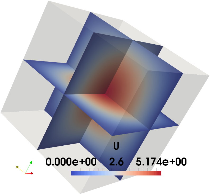
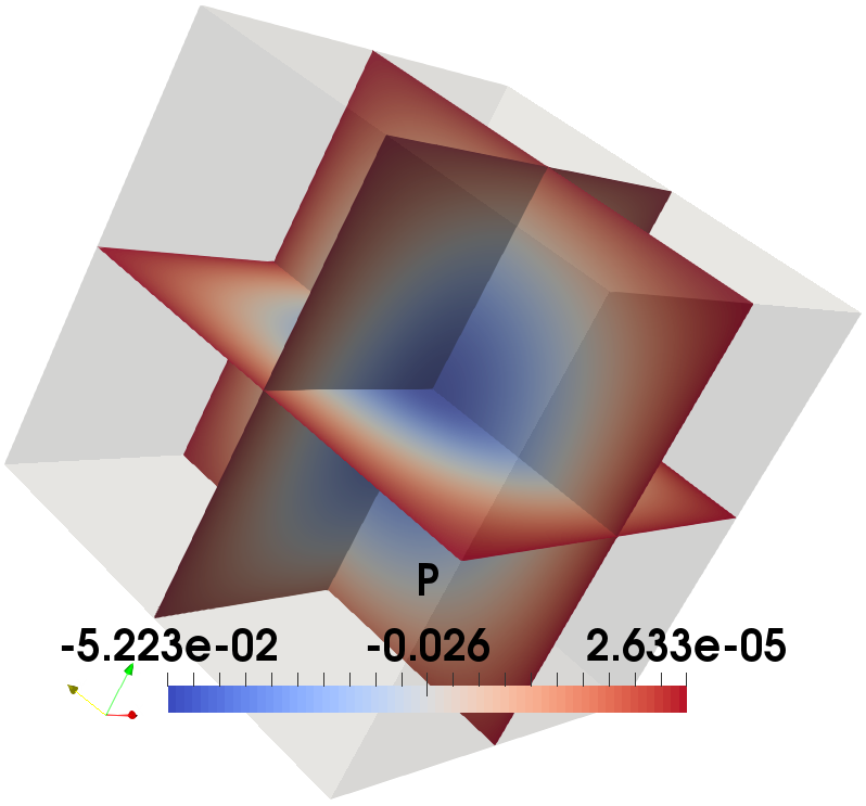
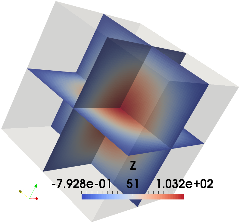
Figure 1: Example 1, numerical solutions of $u$, $p$, and $z$ for the linear model problem using energy regularization.

Table 1: Example 1, estimated order of convergence (eoc) of $u_{h}$ and $p_{h}$ in $Y$.

#Dofs	$h$	$\|u-u_{h}\|_{Y}$	eoc	$\|p-p_{h}\|_{Y}$	eoc
$250$	$1/4$	$4.611e-0$	$-$	$4.651e-2$	$-$
$1,458$	$1/8$	$2.303e-0$	$1.002$	$2.313e-2$	$1.008$
$9,826$	$1/16$	$1.129e-0$	$1.028$	$1.134e-2$	$1.028$
$71,874$	$1/32$	$5.572e-1$	$1.019$	$5.601e-3$	$1.018$
$549,250$	$1/64$	$2.766e-1$	$1.010$	$2.783e-3$	$1.009$
$2,146,689$	$1/128$	$1.379e-1$	$1.005$	$1.388e-3$	$1.004$

Table 2: Example 1, estimated order of convergence (eoc) of $u_{h}$ and $p_{h}$ in $L^{2}(Q)$.

#Dofs	$h$	$\|u-u_{h}\|_{L^{2}(Q)}$	eoc	$\|p-p_{h}\|_{L^{2}(Q)}$	eoc
$250$	$1/4$	$2.365e-1$	$-$	$2.829e-3$	$-$
$1,458$	$1/8$	$5.685e-2$	$2.057$	$7.693e-4$	$1.879$
$9,826$	$1/16$	$1.410e-2$	$2.011$	$2.171e-4$	$1.825$
$71,874$	$1/32$	$3.642e-3$	$1.953$	$6.063e-5$	$1.841$
$549,250$	$1/64$	$9.992e-4$	$1.876$	$1.655e-5$	$1.873$
$2,146,689$	$1/128$	$2.759e-4$	$1.847$	$5.415e-6$	$1.612$

Table 3: Example 1, $J(u_{h},z_{h})$, $|J(u_{h},z_{h})-J(u,z)|$, $J(u,z)=4.53541e-1$.

#Dofs	$h$	$J(u_{h},z_{h})$	$|J(u_{h},z_{h})-J(u,z)|$	eoc
$250$	$1/4$	$5.87348e-1$	$1.3381e-1$	$-$
$1,458$	$1/8$	$4.81288e-1$	$2.7747e-2$	$2.270$
$9,826$	$1/16$	$4.59930e-1$	$6.3890e-3$	$2.119$
$71,874$	$1/32$	$4.55054e-1$	$1.5130e-3$	$2.078$
$549,250$	$1/64$	$4.53863e-1$	$3.2200e-4$	$2.232$
$2,146,689$	$1/128$	$4.53557e-1$	$1.6000e-5$	$4.331$

5.2 An example with a discontinuous target

As in the previous example, we have $\Omega=(0,1)^{2}$, $T=1$, i.e., $Q=(0,1)^{3}$, but now we consider the discontinuous target function

$$u_{d}(x,t)=\begin{cases}&1\quad\text{ if }\sqrt{(x_{1}-\frac{1}{2})^{2}+(x_{2}-\frac{1}{2})^{2}+(t-\frac{1}{2})^{2}}\leq\frac{1}{4},\\ &0\quad\textup{ else.}\end{cases}$$

Here, the regularization parameter is set to $\varrho=10^{-4}$. Following the approach described in [28], we have used a residual based error indicator to drive an adaptive mesh refinement. The space-time finite element solutions for the state $u$ and the adjoint $p$ are provided in Fig. 2 in comparison with the time-dependent target $u_{d}$. The control $z$ is then reconstructed from (14), (15), and (16) by an $L^{2}$ projection on the space of element-wise constant functions. More precisely, we look for an element-wise constant control $z_{h}$ such that

$$\langle z_{h},\varphi_{h}\rangle_{L^{2}(Q)}=-\frac{1}{\varrho}\langle\partial_{t}p_{h}+u_{h}-u_{d},\varphi_{h}\rangle_{L^{2}(Q)}$$

holds for all element-wise constant test functions $\varphi_{h}$. The results are given in the last column of Fig. 2. We clearly see that the control is concentrated near the interface, where the target exhibits a jump. The adaptive mesh is illustrated in Fig. 3 at the $78$th refining step, which contains $3,398,213$ grid points. The total number of degrees of freedom for the coupled state and adjoint equation is $6,796,426$.

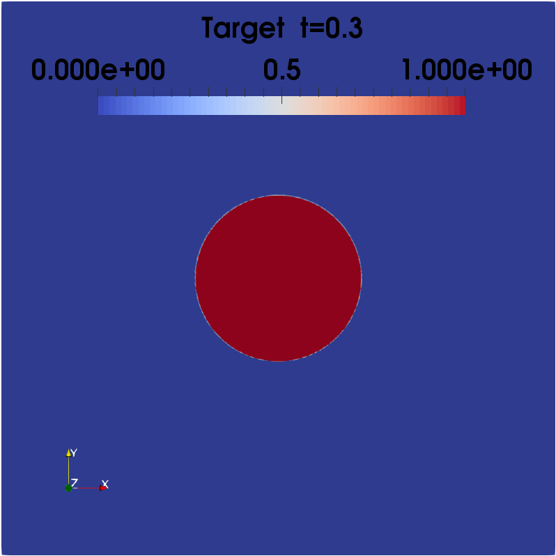
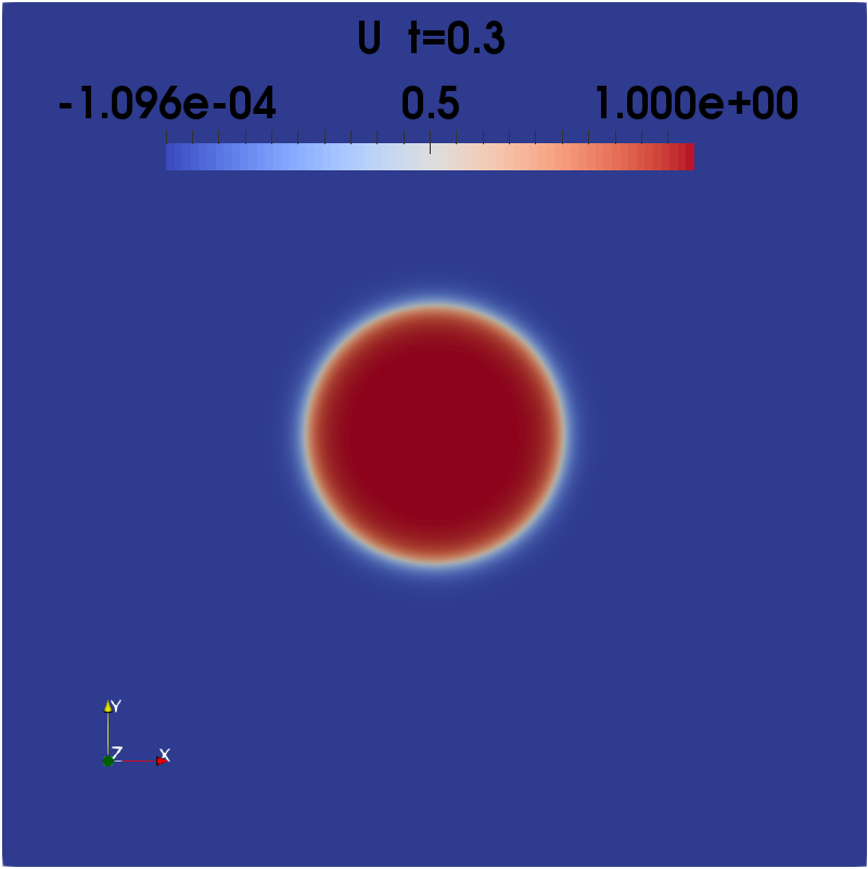
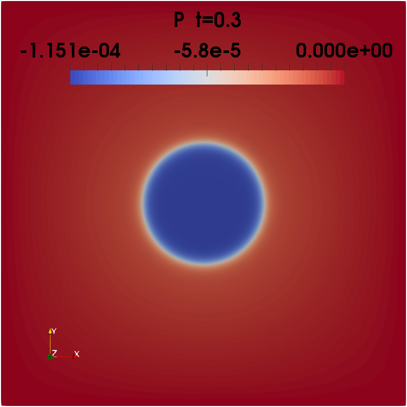
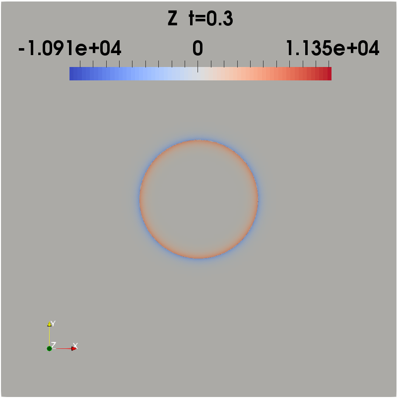
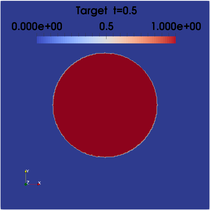
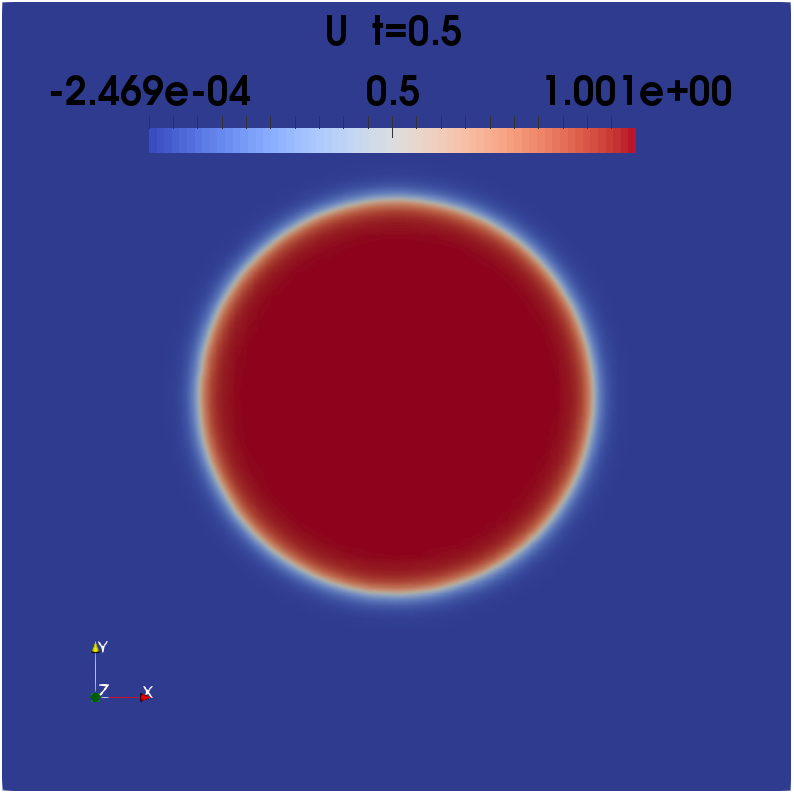
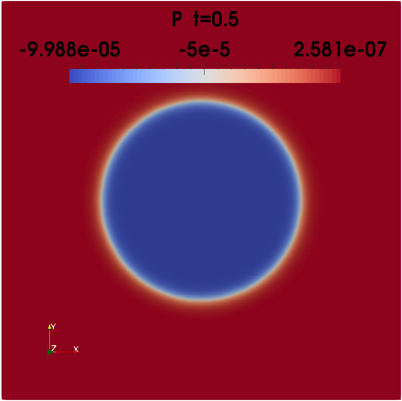
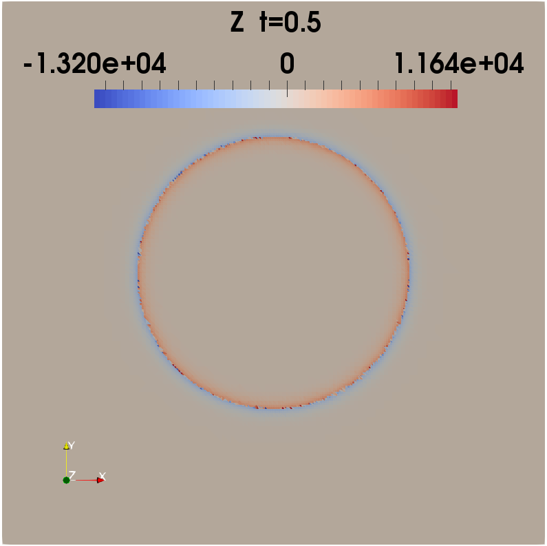
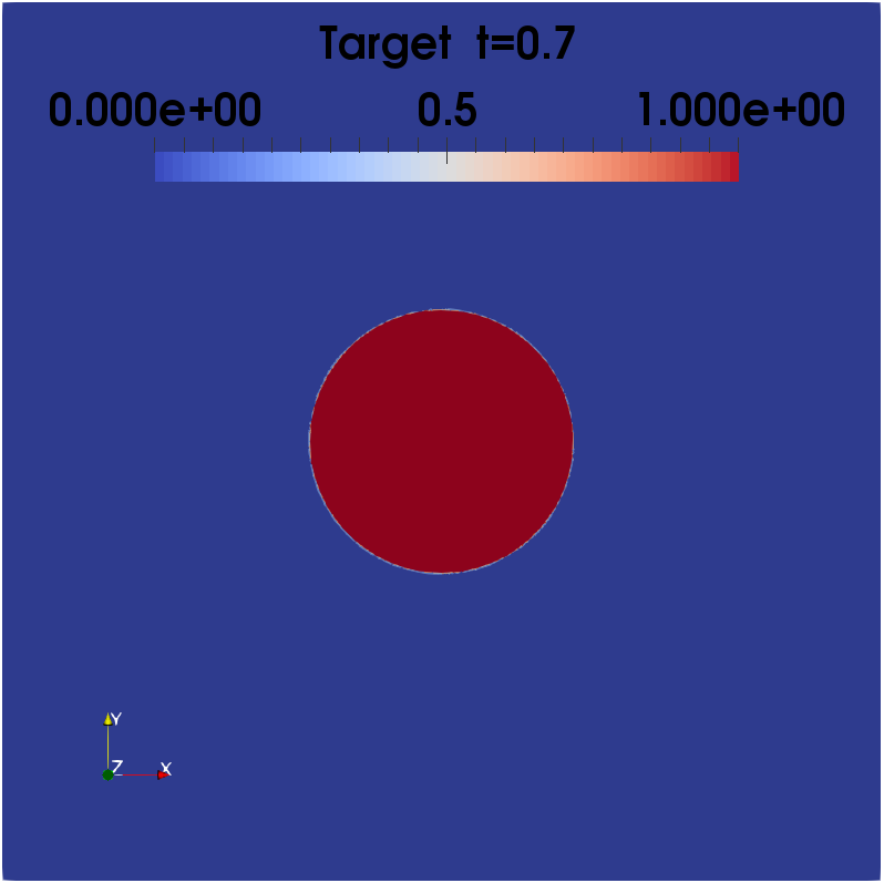
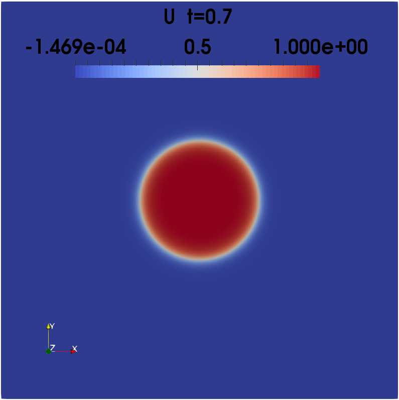
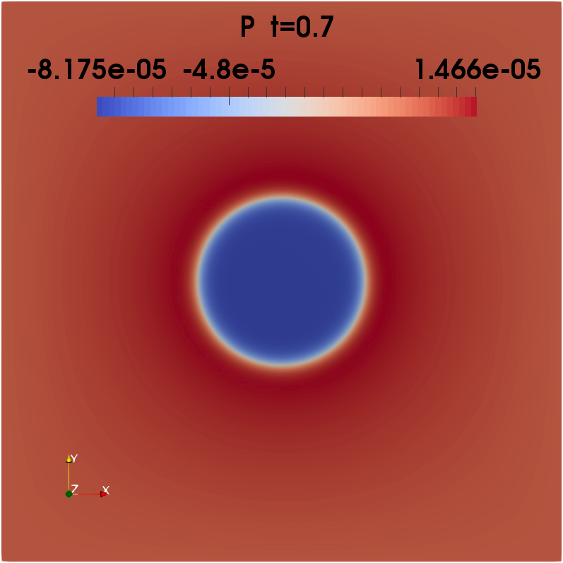
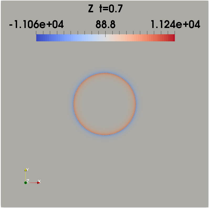
Figure 2: Example 2, Target $u_{d}$ and numerical solutions $u_{h}$, $p_{h}$, and $z_{h}$ for the energy regularization approach with a discontinuous target, at $t=0.3$, $0.5$, and $0.7$ (from top to bottom).

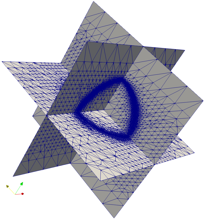
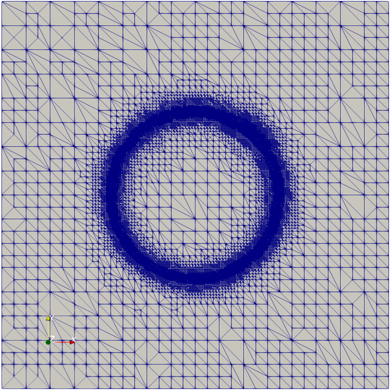
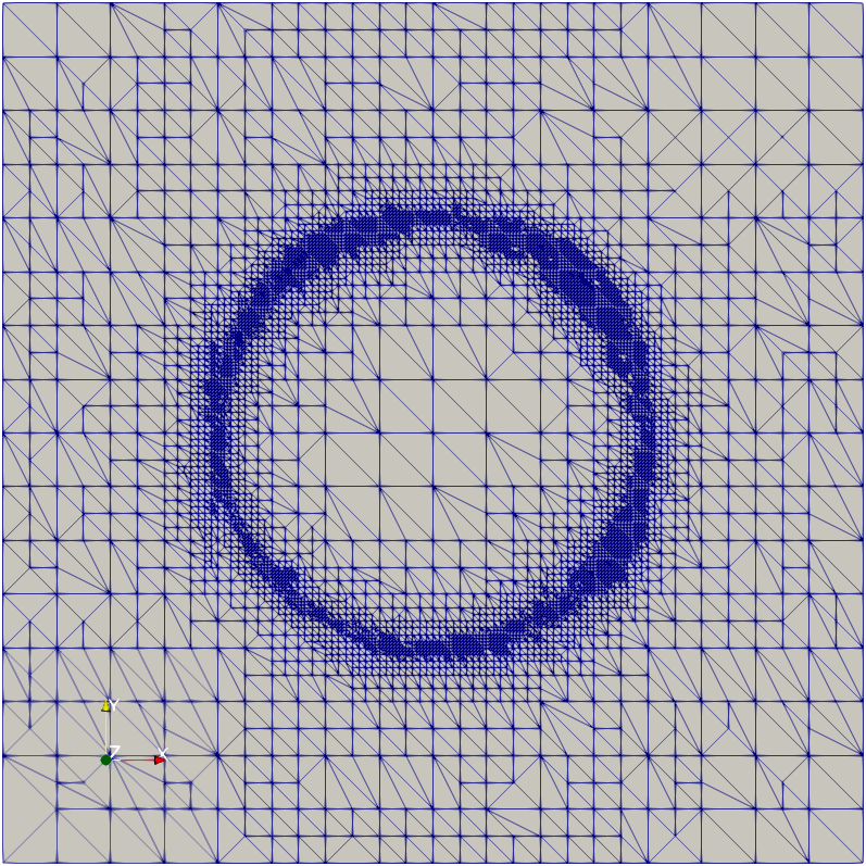
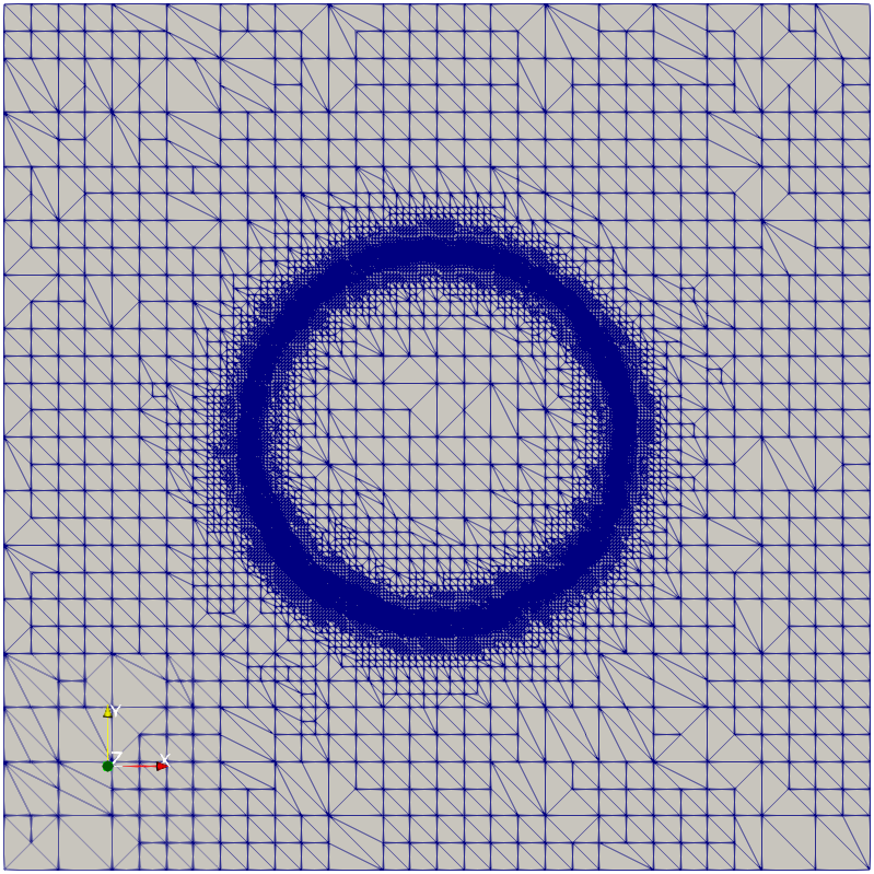
Figure 3: Example 2, Adaptive mesh refinement at the $78$th step in space-time at $t=0.375$, $0.5$, and $0.625$ (from left to right), using energy regularization with a discontinuous target.

Moreover, we also compare the numerical solutions of the energy regularization approach (1) with the solution using $L^{2}$-regularization (3), and with the solution using an $L^{2}+L^{1}$ regularization that promotes spatio-temporal sparsity, i.e., minimize

$${\mathcal{J}}(u,z):=\frac{1}{2}\,\int_{Q}\left|u-u_{d}\right|^{2}\,dx\,dt+\frac{1}{2}\varrho\,\|z\|_{L^{2}(Q)}^{2}+\mu\,\|z\|_{L^{1}(Q)},$$ (25)

subject to (2), and with $\mu>0$. A similar parabolic optimal sparse control model problem has been considered, e.g, in our recent work [19], see also the references given therein.

For all cases, we plot the state $u$ and the control $z$ at $t=0.65$ having a closer look near the interface as depicted in Fig. 4. As predicted, the interface is resolved much sharper, and much less oscillations show up, for the state using the energy regularization than using the $L^{2}$-regularization. With the additional $L^{1}$ term, the state shows less oscillation than pure $L^{2}$-regularization, but a less shaper interface captured than the energy regularization. We further obtain sparser controls by the energy regularization, i.e., the control is non-zero only in a narrow region along the interface, while the control acts in a much larger region near the interface and almost extends to the whole space-time domain by the $L^{2}$-regularization. The $L^{2}+L^{1}$ approach produces a bit spatially sparser solution than the $L^{2}$-regularization, see Fig. 5 for a closer comparison of the control along the line $[0,0.55,0.65]-[1,0.55,0.65]$. All these results are obtained on adaptive meshes that are driven by residual-type error indicators for the coupled optimality system. A comparison of adaptive meshes on the cutting plane $t=0.625$ is illustrated in Fig. 6.

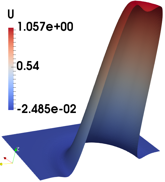
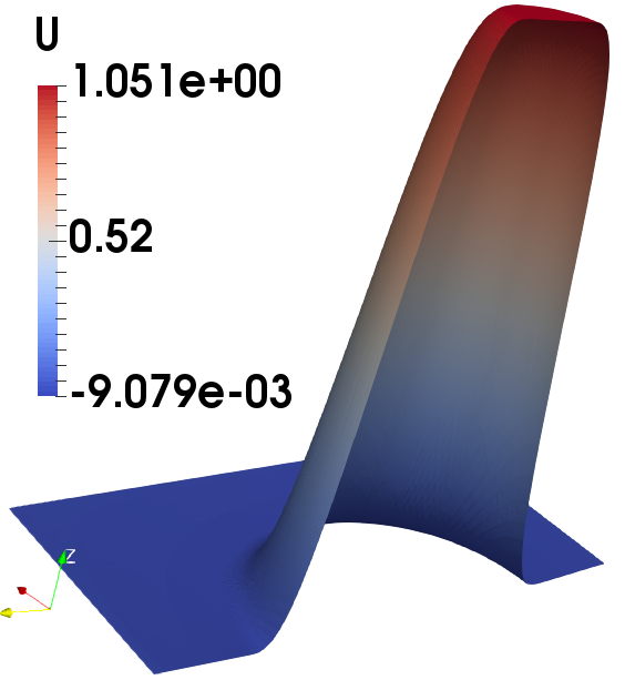
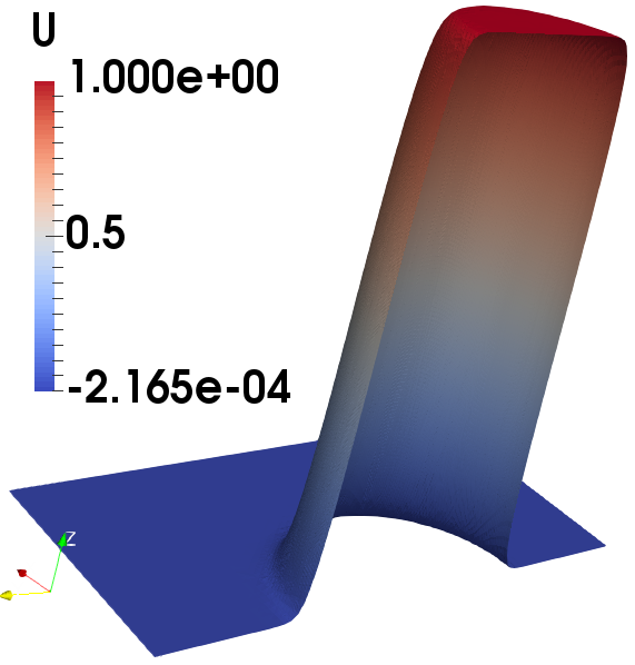
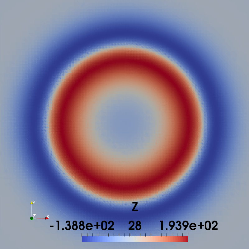
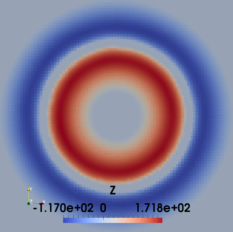
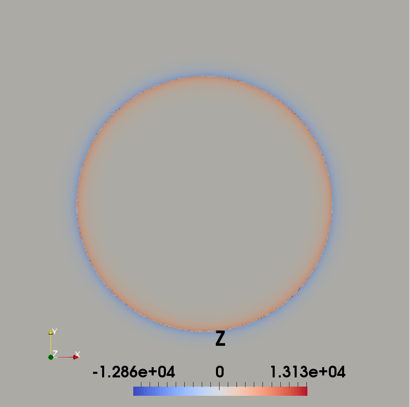
Figure 4: Example 2, Comparison of the numerical solutions of the state $u$ and control $z$ (from top to bottom) at time $t=0.65$, using $L^{2}$-regularization ($\rho=10^{-6}$), $L^{2}+L^{1}$ ($\rho=10^{-6}$, $\mu=10^{-4}$), and energy regularization (from left to right).

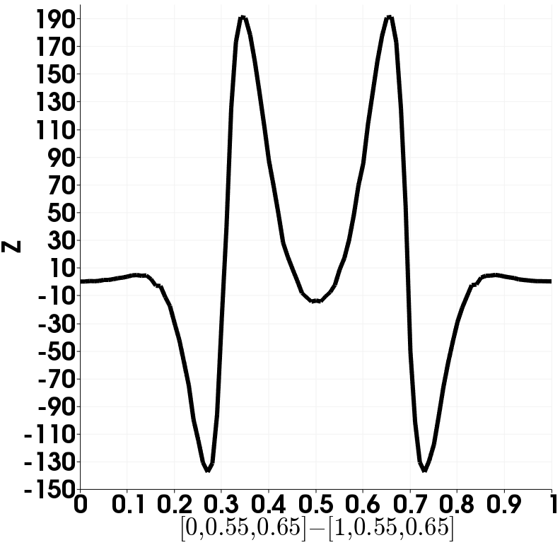
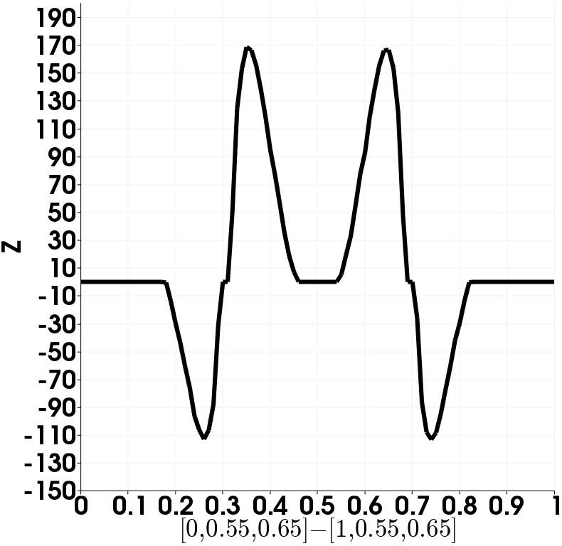
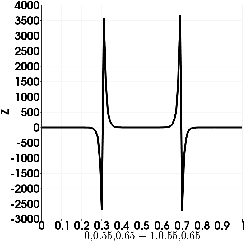
Figure 5: Example 2, Comparison of the numerical solutions of the control $z$ along the line $[0,0.55,0.65]-[1,0.55,0.65]$, using $L^{2}$-regularization ($\rho=1e-6$), $L^{2}+L^{1}$ ($\rho=1e-6$, $\mu=1e-4$), and energy regularization (from left to right).

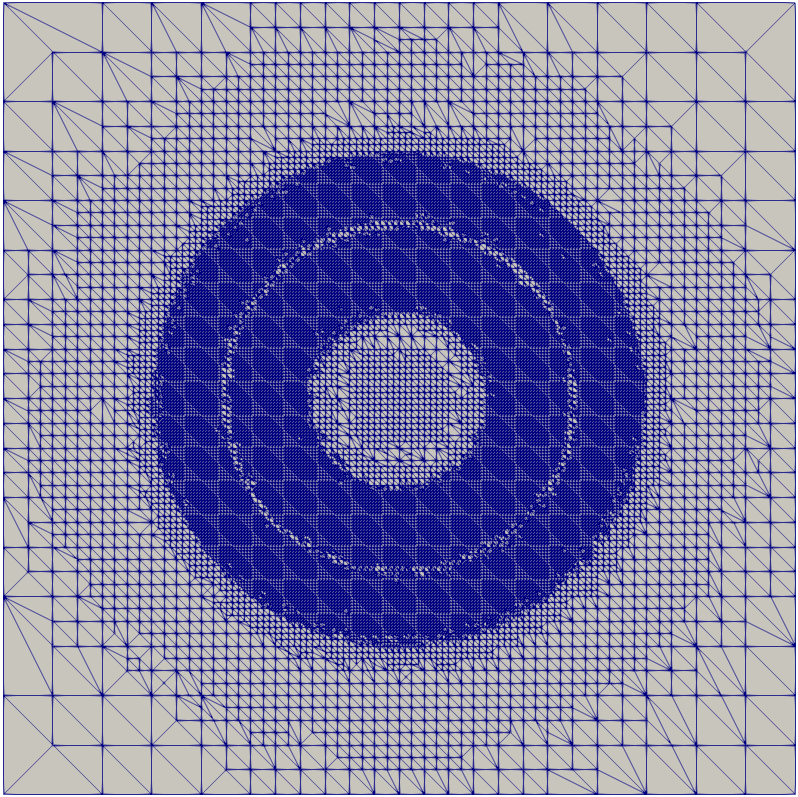
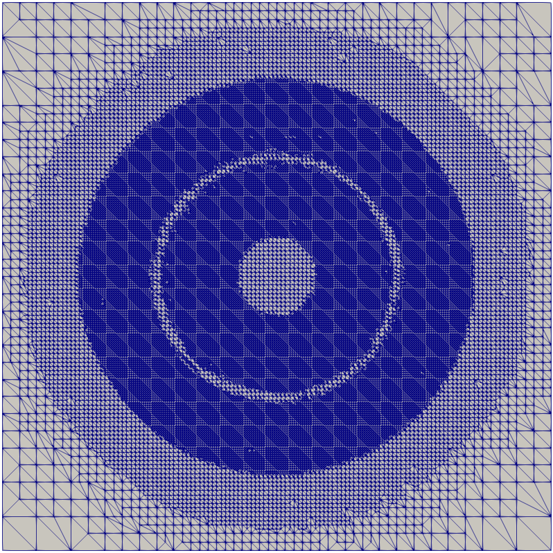
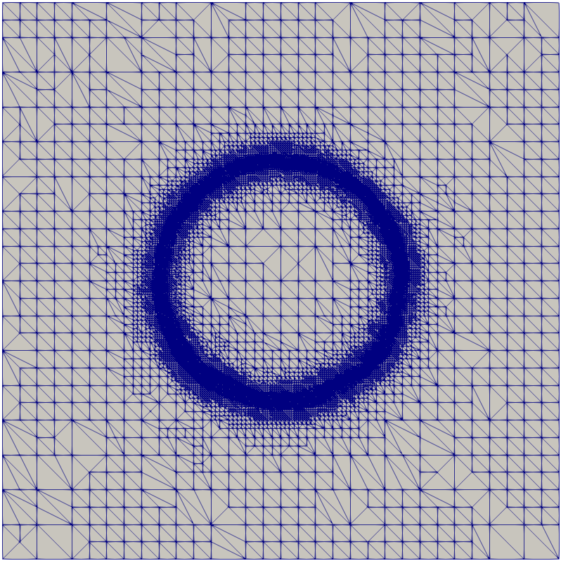
Figure 6: Example 2, Comparison of the adaptive meshes on the cutting plane at time $t=0.625$: $L^{2}$-regularization, $20$th step, $2,080,493$ grid points in space-time (left); $L^{2}+L^{1}$, $23$th step, $3,320,340$ grid points in space-time (middle); energy regularization, $78$th step, $3,398,213$ grid points in space-time (right).

5.3 An example in three space dimensions

Analogous to the example in two space dimensions as considered in Section 5.1, we now construct an example with an explicitly known solution of the first-order optimality system in three space dimensions as follows:

$$u(x,t) =3\pi^{2}\sin(\pi x_{1})\sin(\pi x_{2})\sin(\pi x_{3})\left(et^{2}+t\right),$$

$$p(x,t) =-\varrho\sin(\pi x_{1})\sin(\pi x_{2})\sin(\pi x_{3})\left(at^{2}+bt+1\right),$$

$$z(x,t) =3\pi^{2}\sin(\pi x_{1})\sin(\pi x_{2})\sin(\pi x_{3})\left(at^{2}+bt+1\right),$$

where

$$a=-\frac{9\pi^{4}+3\pi^{2}}{3\pi^{2}+2},\quad b=\frac{9\pi^{4}-2}{3\pi^{2}+2},\quad e=-\frac{3\pi^{2}+1}{3\pi^{2}+2}.$$

When using the adjoint equation, the target is given as $u_{d}=u+\partial_{t}p+\Delta_{x}p$, and we set the regularization parameter $\varrho=0.01$. The numerical solutions $u_{h}$ at $t=1$, $p_{h}$ at $t=0$ and $z_{h}$ at $t=0$ are displayed in Fig. 7.

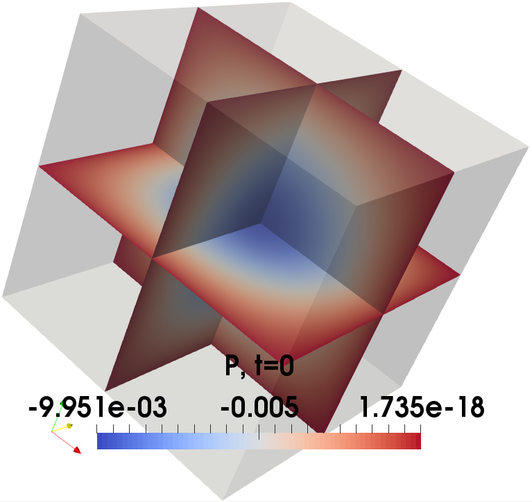
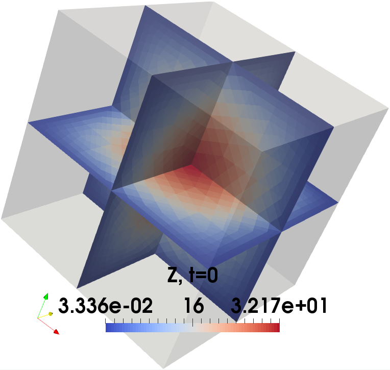
Figure 7: Example 3, numerical solutions $u_{h}$ at $t=1$, $p_{h}$ at $t=0$, and $z_{h}$ at $t=0$ (from left to right).

The error of the space-time finite element approximations $u_{h}$ and $p_{h}$ in the corresponding norms $\|\cdot\|_{Y}$ and $\|\cdot\|_{L^{2}(Q)}$ are given in Table 4 at every second refinement step, see also the error of the objective functional $|J(u,z)-J(u_{h},z_{h})|$ in the last column. In addition, we illustrate the convergence rates in Fig. 8, where we observe optimal rates for the state $u$ and the adjoint state $p$ as already experienced in two space dimensions. Note that, at the finest refinement level, we have $11,171,330$ degrees of freedom in total for the coupled system. The mesh size is approximately $h=0.03125$.

Table 4: Example 3, the error for numerical approximations $u_{h}$, $p_{h}$, and $J_{h}(u_{h},z_{h})$, with $J(u,z)=7.818e-1$.

Lev	#Dofs	$\|u-u_{h}\|_{Y}$	$\|u-u_{h}\|_{L^{2}(Q)}$	$\|p-p_{h}\|_{Y}$	$\|p-p_{h}\|_{L^{2}(Q)}$	$|J-J_{h}|$
$2$	$470$	$5.638e-0$	$3.757e-1$	$5.663e-2$	$3.911e-3$	$2.144e-1$
$4$	$1,430$	$4.988e-0$	$2.927e-1$	$5.012e-2$	$3.096e-3$	$1.648e-1$
$6$	$4,370$	$4.111e-0$	$2.142e-1$	$4.132e-2$	$2.251e-3$	$1.064e-1$
$8$	$18,450$	$3.225e-0$	$1.252e-1$	$3.239e-2$	$1.321e-3$	$5.916e-2$
$10$	$53,186$	$2.187e-0$	$6.349e-2$	$2.195e-2$	$6.648e-4$	$2.559e-2$
$12$	$268,226$	$1.728e-0$	$4.462e-2$	$1.735e-2$	$4.617e-4$	$1.573e-2$
$14$	$744,962$	$1.097e-0$	$1.547e-2$	$1.101e-2$	$1.633e-4$	$6.042e-3$
$16$	$4,103,682$	$8.627e-1$	$1.099e-2$	$8.661e-3$	$1.141e-4$	$3.729e-3$
$18$	$11,171,330$	$5.484e-1$	$3.846e-3$	$5.506e-3$	$4.074e-5$	$1.487e-3$

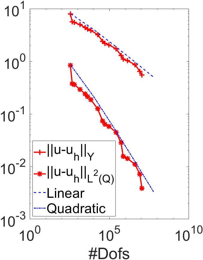
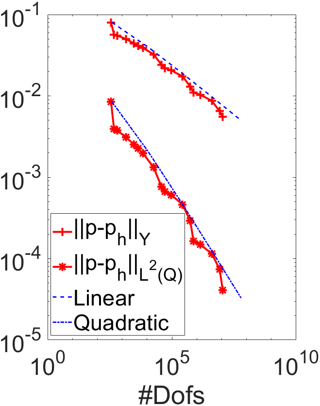
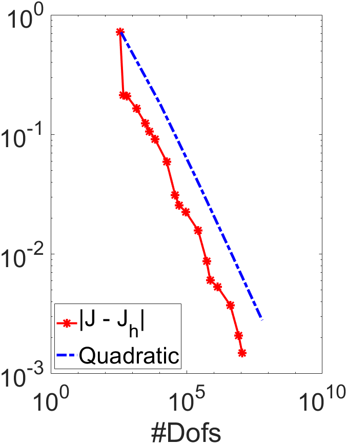
Figure 8: Example 3, convergence history for numerical approximations $u_{h}$, $p_{h}$, and $J_{h}(u_{h},z_{h})$ (from left to right).

6 Conclusions

In this work, we have analyzed space-time finite element methods for the numerical solution of parabolic optimal control problems using energy regulaization in the tracking type objective functional. In contrast to the $L^{2}$ regularization approach as well as the combined $L^{2}+L^{1}$ approach, we observe a more localized control and sharper contours for discontinuous target functions when using energy regularization. In the latter, the discrete optimality system is block skew-symmetric but positive definite, which will allow us to construct optimal preconditioned iterative solution strategies,see, e.g., [25, 26, 34]. Although we only consider the case of unconstrained optimal control problems, this approach can be extended to problems with control constraints and will be considered elsewhere.

References

• [1] A. Alla and S. Volkwein. Asymptotic stability of POD based model predictive control for a semilinear parabolic PDE. Adv. Comput. Math., 41(5):1073–1102, 2015.
• [2] I. Babuška. Error-bounds for finite element method. Numer. Math., 16(4):322–333, 1971.
• [3] I. Babuška and A. Aziz. Survey lectures on the mathematical foundation of the finite element method. In The Mathematical Foundations of the Finite Element Method with Applications to Partial Differential Equations, pages 1–359, New York, 1972. Academic Press.
• [4] J. Bey. Tetrahedral grid refinement. Computing, 55:355–378, 1995.
• [5] A. Borzì and V. Schulz. Computational optimization of systems governed by partial differential equations, volume 8 of Computational Science & Engineering. Society for Industrial and Applied Mathematics (SIAM), 2011.
• [6] D. Braess. Finite Elements: Theory, Fast Solvers, and Applications in Solid Mechanics. Cambridge University Press, Cambridge, 2007.
• [7] A. Bünger, S. Dolgov, and M. Stoll. A low-rank tensor method for PDE-constrained optimization with isogeometric analysis. SIAM J. Sci. Comput., 42(1):A140–A161, 2020.
• [8] A. Ern and J.-L. Guermond. Theory and Practice of Finite Elements. Springer-Verlag, New Year, 2004.
• [9] M. J. Gander. 50 years of time parallel integration. In Multiple Shooting and Time Domain Decomposition, pages 69–114. Springer Verlag, Heidelberg, Berlin, 2015.
• [10] W. Gong, M. Hinze, and Z. Zhou. Space-time finite element approximation of parabolic optimal control problems. J. Numer. Math., 20(2):111–145, 2012.
• [11] M. Gunzburger and A. Kunoth. Space-time adaptive wavelet methods for optimal control problems constrained by parabolic evolution equations. SIAM J. Control Optim., 49(3):1150–1170, 2011.
• [12] M. Hinze, R. Pinnau, M. Ulbrich, and S. Ulbrich. Optimization with PDE Constraints, volume 23. Springer-Verlag, Berlin, 2009.
• [13] M. Kollmann, M. Kolmbauer, U. Langer, M. Wolfmayr, and W. Zulehner. A finite element solver for a multiharmonic parabolic optimal control problem. Comput. Math. Appl., 65:469–486, 2013.
• [14] O. A. Ladyzhenskaya. The boundary value problems of mathematical physics, volume 49 of Applied Mathematical Sciences. Springer-Verlag, New York, 1985. Translated from the Russian edition, Nauka, Moscow, 1973.
• [15] O. A. Ladyzhenskaya, V. A. Solonnikov, and N. Uraltseva. Linear and quasi-linear equations of parabolic type. AMS, USA, 1968. Translated from the Russian edition, Nauka, Moscow, 1967.
• [16] J. Lang. Adaptive Multilevel Solution of Nonlinear Parabolic PDE Systems. Theory, Algorithm, and Applications, volume 16 of Lecture Notes in Computational Sciences and Engineering. Springer Verlag, Heidelberg, Berlin, 2000.
• [17] U. Langer, S. Repin, and M. Wolfmayr. Functional a posteriori error estimates for time-periodic parabolic optimal control problems. Numer. Func. Anal. Opt., 37(10):1267–1294, 2016.
• [18] U. Langer, O. Steinbach, F. Tröltzsch, and H. Yang. Unstructured space-time finite element methods for optimal control of parabolic equations. Technical Report arXiv:2004.02014 [math.NA], arXiv, 2020.
• [19] U. Langer, O. Steinbach, F. Tröltzsch, and H. Yang. Unstructured space-time finite element methods for optimal sparse control of parabolic equations. Technical Report arXiv:2003.14141 [math.NA], arXiv, 2020.
• [20] J. L. Lions. Contrôle optimal de systèmes gouvernés par des équations aux dérivées partielles. Dunod Gauthier-Villars, Paris, 1968.
• [21] D. Meidner and B. Vexler. A priori error estimates for space-time finite element discretization of parabolic optimal control problems. Part I: Problems without control constraints. SIAM J. Control Optim., 47(3):1150–1177, 2008.
• [22] D. Meidner and B. Vexler. A priori error estimates for space-time finite element discretization of parabolic optimal control problems. Part II: Problems with control constraints. SIAM J. Control Optim., 47(3):1301–1329, 2008.
• [23] M. Neumüller. Eine Finite Elemente Methode für optimale Kontrollprobleme mit parabolischen Randwertaufgaben. Master’s thesis, TU Graz, 2010.
• [24] J. Nečas. Sur une méthode pour résoudre les équations aux dérivées partielles du type elliptique, voisine de la variationnelle. Ann. Scuola Norm. Sup. Pisa, 16(4):305–326, 1962.
• [25] A. Schiela and S. Ulbrich. Operator preconditioning for a class of inequality constrained optimal control problems. SIAM J. Optim., 24(1):435–466, 2014.
• [26] V. Schulz and G. Wittum. Transforming smoothers for PDE constrained optimization problems. Comput Visual Sci (, 11:207–219, 2008.
• [27] O. Steinbach. Space-time finite element methods for parabolic problems. Comput. Methods Appl. Math., 15:551–566, 2015.
• [28] O. Steinbach and H. Yang. Comparison of algebraic multigrid methods for an adaptive space-time finite-element discretization of the heat equation in 3d and 4d. Numer. Linear Algebra Appl., 25(3):e2143, 2018.
• [29] O. Steinbach and H. Yang. Space-time finite element methods for parabolic evolution equations: discretization, a posteriori error estimation, adaptivity and solution. In O. Steinbach and U. Langer, editors, Space-Time Methods: Application to Partial Differential Equations, Radon Series on Computational and Applied Mathematics, pages 207–248, Berlin, 2019. de Gruyter.
• [30] R. Stevenson. The completion of locally refined simplicial partitions created by bisection. Math. Comput., 77(261):227–241, 2008.
• [31] V. Thomée. Galerkin finite element methods for parabolic problems, volume 25 of Springer Series in Computational Mathematics. Springer-Verlag, Berlin, second edition, 2006.
• [32] F. Tröltzsch. Optimal control of partial differential equations: Theory, methods and applications, volume 112 of Graduate Studies in Mathematics. American Mathematical Society, Providence, Rhode Island, 2010.
• [33] E. Zeidler. Nonlinear Functional Analysis and its Applications II/B: Nonlinear Monotone Operators. Springer, New York, 1990.
• [34] W. Zulehner. Nonstandard norms and robust estimates for saddle point problems. SIAM J. Matrix Anal. Appl., 32(2):536–560, 2011.