The Ultraluminous Ly$\alpha$ Luminosity Function at $z=6.6$

Abstract

We present the luminosity function (LF) for ultraluminous Ly$\alpha$ emitting galaxies (LAEs) at $z=6.6$. We define ultraluminous LAEs (ULLAEs) as galaxies with $\log L(\textrm{Ly}\alpha)>43.5$ erg s^-1. We select our main sample using the $g^{\prime}$, $r^{\prime}$, $i^{\prime}$, $z^{\prime}$, and NB921 observations of a wide-area (30 deg²) Hyper Suprime-Cam survey of the North Ecliptic Pole (NEP) field. We select candidates with $g^{\prime},r^{\prime},i^{\prime}>26$, NB$921\leq 23.5$, and NB$921-z^{\prime}\leq 1.3$. Using the DEIMOS spectrograph on Keck II, we confirm 9 of our 14 candidates as ULLAEs at $z=6.6$ and the remaining 5 as an AGN at $z=6.6$, two [OIII]$\lambda$5007 emitting galaxies at $z=0.84$ and $z=0.85$, and two non-detections. This emphasizes the need for full spectroscopic follow-up to determine accurate LFs. In constructing the ULLAE LF at $z=6.6$, we combine our 9 NEP ULLAEs with two previously discovered and confirmed ULLAEs in the COSMOS field: CR7 and COLA1. We apply rigorous corrections for incompleteness based on simulations. We compare our ULLAE LF at $z=6.6$ with LFs at $z=5.7$ and $z=6.6$ from the literature. Our data reject some previous LF normalizations and power law indices, but they are broadly consistent with others. Indeed, a comparative analysis of the different literature LFs suggests that none is fully consistent with any of the others, making it critical to determine the evolution from $z=5.7$ to $z=6.6$ using LFs constructed in exactly the same way at both redshifts.

1 Introduction

The epoch of reionization, in which the intergalactic medium (IGM) transitioned from being dominantly neutral to being primarily ionized, is a key era in the universe’s history. Ly$\alpha$ emission from early, massively star-forming galaxies is one of the few probes of galaxy evolution and activity in this era. This early Ly$\alpha$ emission is redshifted from the rest-frame UV into the observed-frame optical, whereas other less energetic diagnostic emission lines are redshifted into the more difficult to observe infrared.

Narrowband ($\sim 100$ Å) surveys can identify Ly$\alpha$ emitter (LAE) candidates at specific redshifts by imaging low-background windows in the atmospheric sky. In recent years, narrowband surveys have identified LAE candidates out to redshifts beyond $z=7$ (e.g., Hu et al., 2004, 2010, 2016; Ouchi et al., 2008, 2010; Kashikawa et al., 2011; Konno et al., 2014, 2018; Matthee et al., 2015; Santos et al., 2016; Jiang et al., 2017; Ota et al., 2017; Songaila et al., 2018; Itoh et al., 2018; Hu et al., 2019). With this large influx of new samples, the very high-redshift Ly$\alpha$ luminosity function (LF) is being probed. However, most of these LFs suffer from low number statistics and large errors, especially at the ultraluminous ($\log L(\textrm{Ly}\alpha)>43.5$ erg s^-1) end. The rarity of ultraluminous LAEs (ULLAEs) makes the population highly susceptible to contamination from foreground strong emission line galaxies and from active galactic nuclei (AGNs), which means spectroscopic confirmation is critical. Additionally, wide-area surveys are needed to reduce possible effects of cosmic variance.

The evolution of the LAE LF potentially offers insight into the onset of reionization. In particular, Santos et al. (2016) have claimed to see differential evolution in the shape of the LAE LF at high redshift, i.e., a significant decline in the number density of “typical” LAEs from $z=5.7$ to $z=6.6$, and no evolution of ULLAEs over the same redshift range. Such a result might imply that reionization is being completed first around ULLAEs, since the increasing neutrality would have a larger effect on the luminosities of the lower luminosity LAEs than on those of the ULLAEs. Moreover, it would be consistent with the interpretation of the discovery of some complex line profiles for $z=6.6$ ULLAEs (Hu et al., 2016; Songaila et al., 2018) as possible evidence for ULLAEs generating highly ionized regions of the IGM in their vicinity, thereby allowing the full Ly$\alpha$ profile of the galaxy, including blue wings, to become visible.

Suprime-Cam and Hyper Suprime-Cam (HSC) narrowband surveys (e.g., Ouchi et al., 2008, 2010; Hu et al., 2010; Kashikawa et al., 2011; Matthee et al., 2015; Santos et al., 2016; Zheng et al., 2017; Konno et al., 2018) are not all in agreement on the evolution of the LFs, though generally a decrease from $z=5.7$ to $z=6.6$ for non-ULLAEs is claimed. Most of these surveys (other than the spectroscopically complete survey of Hu et al., 2010) have relatively few spectroscopic redshifts, and the measured values at the ultraluminous end, when they exist at all, typically have large uncertainties. Without spectroscopy, contaminants are likely to be included in the LAE samples, which will result in higher normalizations for the LFs. There is also the issue of incompleteness corrections. For Suprime-Cam, the filters are far from top-hat. Thus, without knowing the exact redshift of a source, and hence where it lies in the filter, it is very difficult to correct the Ly$\alpha$ luminosity for the effect of the filter transmission profile. This will impact the number densities of bright LAEs, as some of these will be observed at a fraction of their luminosities. In addition, some fainter LAEs will fall below the selection magnitude limit and hence not be included in the sample. For HSC, the more top-hat like filters lessen these effects, but corrections are still needed.

On the other hand, it was pointed out by Kashikawa et al. (2011) that spectroscopically complete samples could result in lower normalizations for the LFs if insufficiently deep spectral data are used for the Ly$\alpha$ line identifications, since some candidates from the initial selection might be incorrectly removed.

The goal of the present paper is to construct the ULLAE portion of the LF at $z=6.6$ using a spectroscopically complete sample with sufficiently deep spectra that there is no ambiguity about the redshift identifications. This prevents the sample from being contaminated by non-LAEs, and it also means that the Ly$\alpha$ luminosity corrections due to the filter transmission profile are exact.

Hu et al. (2016) obtained narrowband NB921 images with HSC of the COSMOS field, and Songaila et al. (2018) did the same for a much larger area in the North Ecliptic Pole (NEP) field. From these data, we now have 11 spectroscopically confirmed ULLAEs at $z=6.6$ from which to construct the ultraluminous end of the LF. We will then make comparisons of this new ULLAE LF with LAE LFs at $z=5.7$ and $z=6.6$ from the literature.

We assume $\Omega_{\rm M}$=0.3, $\Omega_{\Lambda}$=0.7, and H₀=70 km s^-1 Mpc^-1 throughout. We give all magnitudes in the AB magnitude system, where an AB magnitude is defined by $m_{AB}=-2.5\log f_{\nu}-48.60$. We define $f_{\nu}$, the flux of the source, in units of erg cm^-2 s^-1 Hz^-1.

2 Candidate Selection

We use data from the Hawaii eROSITA Ecliptic Pole Survey, or HEROES, a 45 deg² imaging survey of the North Ecliptic Pole (NEP; dashed line in Figure 1; see Songaila et al. 2018). HEROES consists of Subaru 8.2 m HSC broadband $g^{\prime}$, $r^{\prime}$, $i^{\prime}$, $z^{\prime}$, and $y^{\prime}$ and narrowband NB816 and NB921 imaging. (The $r^{\prime}$ and $i^{\prime}$ filters are the HSC-r2 and HSC-i2 filters.) HEROES also includes $U$ and $J$ imaging from the Canada-France-Hawaii Telescope (CFHT) 3.6 m MegaPrime/MegaCam and WIRCam instruments. In this work, we only use the $g^{\prime}$, $r^{\prime}$, $i^{\prime}$, $z^{\prime}$, and NB921 data, and we focus on the most uniformly covered area, which is 30 deg² in size (black rectangle in Figure 1). For the NB921 data, the $1\sigma$ noise in a $2^{\prime\prime}$ diameter aperture ranges from 25.4–26.1. For the $z^{\prime}$-band data, the $1\sigma$ noise in a $2^{\prime\prime}$ diameter aperture ranges from 26.2–27.0. A detailed discussion of both the observations and the data reduction with the Pan-STARRS Image Processing Pipeline (Magnier et al., 2016) can be found in Songaila et al. (2018).

Songaila et al. (2018) selected objects with NB921 Kron magnitudes brighter than 23.5 in the 30 deg² area. This selection in NB921 provides a $>5\sigma$ criterion throughout the area and a much higher signal-to-noise (mean of $9\sigma$) through most of the area. This yielded a sample of 2.8 million objects. For these objects, they centered on the NB921 positions and measured the magnitudes across the filters using $2^{\prime\prime}$ diameter apertures. They then restricted to sources with $z^{\prime}$–NB921 $\geq 1.3$ that were also not detected above the 2$\sigma$ level in any of the $g^{\prime}$, $r^{\prime}$ and $i^{\prime}$ bands, as would be expected for LAEs with a strong Lyman break. The $z^{\prime}$–NB921 $\geq 1.3$ color excess selects high equivalent width spectra (observed-frame EW(Ly$\alpha$) $>100$ Å) at redshifts $6.50<z<6.63$. This choice of color excess selects all galaxies with rest-frame EW(Ly$\alpha$) $\geq 20$ Å, which is the normal definition of a high-redshift LAE (Hu et al., 1998). Lyman continuum break sources at redshifts placing the break near the upper wavelength of the narrowband filter can also satisfy these selection criteria, again emphasizing the need for spectroscopic follow-up. We summarize our selection criteria in Table 1.

We reanalyzed the selected candidates, looking for contamination from glints, bright stars, moving objects, etc. We then stacked the $g^{\prime}$, $r^{\prime}$, and $i^{\prime}$ images for each of the remaining candidates and discarded any sources that appeared in both the narrowband and stacked images. After our reanalysis, we ended up with 14 candidates for spectroscopic followup, 13 of which are in common with Songaila et al. (2018).

Table 1: Photometric Selection Criteria

Filter	Selection
$g^{\prime}$	$>26$
$r^{\prime}$	$>26$
$i^{\prime}$	$>26$
NB921	$\leq 23.5$
$z^{\prime}-\textrm{NB921}$	$\geq 1.3$

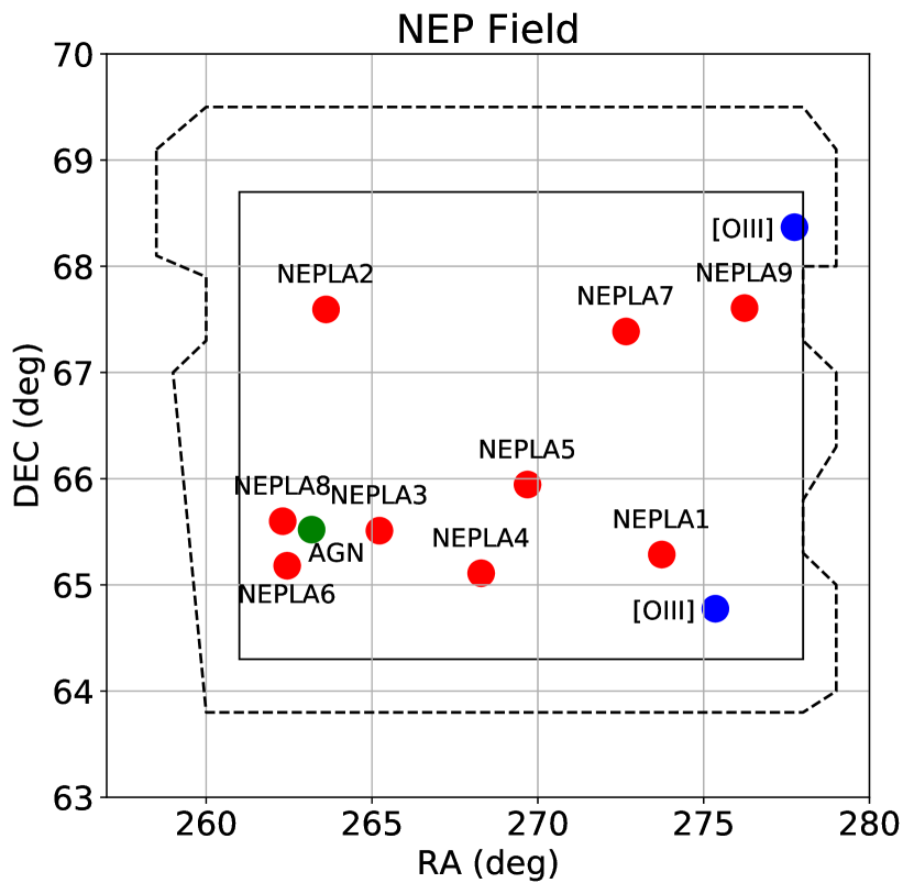
Figure 1: The dashed line shows the full $\sim$45 deg² of the current HEROES survey, and the solid rectangle shows the most uniformly covered 30 deg² area studied in this work. Red circles denote the positions of the 9 spectroscopically confirmed LAEs, blue circles indicate the two [OIII] emitters, and the green circle indicates the single AGN. There were also two candidates that turned out to be spurious after spectroscopic observations.

3 Spectroscopic Follow-Up

Songaila et al. (2018) spectroscopically followed up 7 of the candidates, and we followed up the remaining 7 with DEIMOS on Keck II during observing runs in 2018 and 2019. We refer the reader to A. Songaila et al. (2020, in preparation), where we provide a more detailed description of the data and analysis of the spectra. Briefly, we used the G830 grating with a $1^{\prime\prime}$ slit, which results in a resolution of 83 km s^-1 for the $z=6.6$ LAEs, as measured from sky lines. We took three 20 minute sub-exposures for each source using $\pm 1.5^{\prime\prime}$ dithering along the slit for optimal sky subtraction. Our total exposure times ranged from 1–3 hours, depending on the source.

We carried out the data reduction using the standard pipeline presented in Cowie et al. (1996). In short, we performed an initial sky subtraction, pixel by pixel, using the minimum counts recorded by a pixel across the three dithered exposures. We then median added the three frames. We rejected cosmic rays using a $3\times 3$ median spatial filtering pass. We removed geometric distortion from the spectra by tracing brighter objects in the slit mask. We then calibrated the wavelength scales against the sky lines in the spectra. Finally, we performed another sky subtraction. We show a range of two-dimensional (2D) spectral images for our sample in Figure 2, including a spectroscopic non-detection, an [OIII] emitter, the single detected AGN (NEPAGN), the double-peaked ULLAE NELPA4, and two other ULLAEs: NEPLA1 (the most luminous ULLAE in the sample) and NEPLA8 (the second least luminous ULLAE in the sample).

In total, we confirmed 9 NEP candidates as $z=6.6$ ULLAEs. We present the one-dimensional (1D) spectra of all 9 in Figure 3. As in Songaila et al. (2018), for each profile, we chose the peak value of the Ly$\alpha$ line in the 1D spectrum as the zero-velocity standard from which to calculate the spectroscopic redshift. This is not the galaxy redshift, which may be blueward of this value. For example, for the LAE VR7, the Ly$\alpha$ flux peaks at $z=6.534\pm 0.001$ (Matthee et al., 2020), which corresponds to a velocity offset of $+213^{+19}_{-20}$ km s^-1 relative to the systemic redshift traced by [CII]${}_{\rm 158~{}\mu m}$ ($z=6.5285$; Matthee et al. 2019). The peak redshifts allow us to compare the redshifts of the sample and are adequate for calculating the transmission throughput needed for determining the line fluxes.

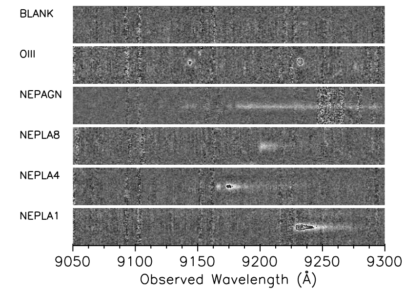
Figure 2: 2D spectra for six $z=6.6$ LAE candidates with comparable NB921 magnitudes. The top spectrum has no detected lines and is one of the two spectroscopic non-detections. The second spectrum is one of the two [OIII] emitters, with the [OIII] doublet and fainter H$\beta$ line visible. The third spectrum is the single AGN, featuring a bright continuum with no Ly$\alpha$ line emission. The fourth spectrum is an example of a confirmed ULLAE spectrum (NEPLA8) with strong Ly$\alpha$ emission featuring a sharp blue break and a red wing. It is one of the least luminous ULLAEs in the sample. The fifth spectrum is the double-peaked ULLAE NEPLA4. The bottom spectrum is the most luminous confirmed ULLAE so far, NEPLA1.

We identified one of the remaining 5 candidates as a $z=6.6$ AGN (see the 1D spectrum in Songaila et al., 2018). This spectrum shows broad Ly$\alpha$ emission, along with OVI and NV. We identified two other candidates as high EW [OIII]$\lambda$5007 emitters at $z=0.84$ and $z=0.85$. The continuum in these sources is not detected in any of the blue bandpasses, making this type of source hard to remove with a purely photometric selection. The spectra only show the [OIII] doublet and H$\beta$ line, in each case with both of the [OIII] lines being much stronger than the H$\beta$ line (see the second spectrum in Figure 2). [OIII] emitters are cited as leading sources of contamination in photometrically identified LAE samples (Konno et al., 2018). Finally, we did not detect any lines in the last two candidates.

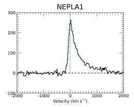
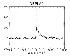
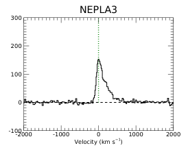
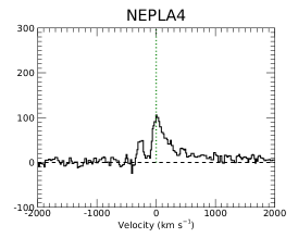
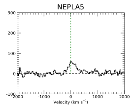
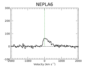
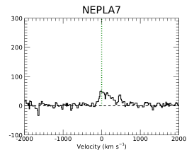
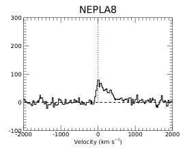
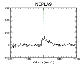
Figure 3: 1D spectra of the nine confirmed $z=6.6$ ULLAEs in the NEP field. The vertical scale is the flux in arbitrary units, but these are consistent between the spectra, so the normalizations can be directly compared.

Characterizing the noise in the spectral images is not straightforward, because of the presence of the residuals from the sky subtraction. However, the spectra with detected lines are clearly distinguishable from the two spectra without (see Figure 2). In order to quantify this, we used box apertures in the 2D spectra with 30 spectral pixels and 10 spatial pixels to measure the distribution of counts in the wavelength region covered by the NB921 filter and lying within $3^{\prime\prime}$ of the nominal position for the NEP candidates. We then compared the largest value measured in any of these apertures with the dispersion. Typically, the S/N of detected Ly$\alpha$ lines is in excess of 10, while that of [OIII]$\lambda$5007 lines is greater than 8. For the two spectra without detected lines, we did not see boxes with S/N greater than 2. Thus, these two sources are clearly spurious, and the normalization of our LF will not be artificially lowered due to their removal from the initial sample.

We note that it is also possible to confirm the reality of the LAEs with broadband continuum data in $z^{\prime}$ and $y^{\prime}$, but the continuum data for the NEP field are not deep enough to do this.

Our follow-up success rate for ULLAEs in the NEP 30 deg² area is thus 64%. This illustrates how critical spectroscopic follow-up is for the confirmation of bonafide ULLAEs and the filtration of contaminants. We supplement our 9 NEP ULLAEs with two ULLAEs from the COSMOS field: COLA1 (Hu et al., 2016) and CR7 (Sobral et al., 2015). COLA1 and CR7 are a spectroscopically complete ULLAE sample observed in the same DEIMOS configuration as the NEP sources (Songaila et al., 2018).

We note that Songaila et al. (2018) also targeted the LAE MASOSA (Sobral et al., 2015) in COSMOS. However, its luminosity of $\log L(\rm Ly\alpha)=43.42$ erg s^-1 lies just below the ULLAE luminosity limit, so we do not include it in this study.

4 Line Fluxes and Luminosities

A primary purpose of this study is to explore the ultraluminous tail of the $z=6.6$ LAE LF. As all of our LAEs are spectroscopically confirmed, we have the advantage over other works of accurate spectroscopic redshifts and Ly$\alpha$ observed wavelengths. In Figure 4, we show the redshifts and observed Ly$\alpha$ wavelengths for the NEP and COSMOS sources with the HSC filter profiles superimposed.

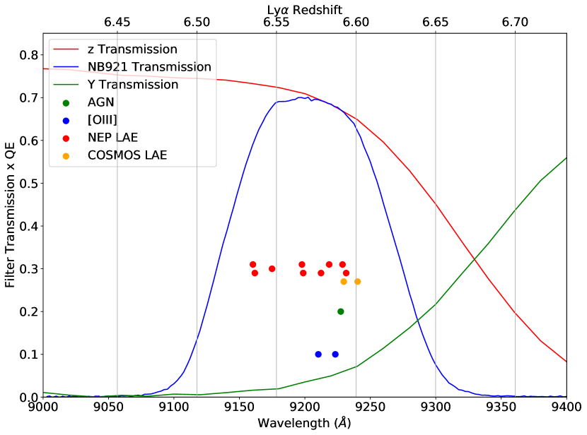
Figure 4: Product of the filter transmission and CCD quantum efficiency for the HSC filters $z$ (red), NB921 (blue), and $Y$ (green). Red (orange) circles show the redshift and observed redshifted peak Ly$\alpha$ wavelength for each NEP (COSMOS) ULLAE. Blue circles show the weighted mean wavelength of the [OIII] doublet for the two [OIII] emitters. The single green circle is a high-redshift AGN. Vertical offsets are simply used to distinguish overlapping points.

To calculate the Ly$\alpha$ line flux, we first measured the NB921 magnitude of each LAE using a $2^{\prime\prime}$ diameter aperture. We then corrected this magnitude to a total magnitude using the median offset between $2^{\prime\prime}$ and $4^{\prime\prime}$ diameter aperture measurements of galaxies in the 22–24 magnitude range in the neighborhood of the source (typically around $-0.2$ mag). A. Songaila et al. (2020, in preparation) describe the conversion of these NB921 magnitudes to Ly$\alpha$ line fluxes by assuming that the NB921 flux is produced solely by the Ly$\alpha$ line. They also find that if one includes the continuum, then it reduces the Ly$\alpha$ flux and luminosity by a very small amount, typically substantially less than 0.1 dex. However, we do not have deep enough continuum data in the NEP to do this accurately.

Finally, we calculated the line luminosity of each LAE using the cosmological luminosity distance based on its spectroscopic redshift.

In Table 2, we present the final catalog of the 9 NEP LAEs, the 2 COSMOS LAES, the NEP AGN, and the 2 [OIII] emitters. All 9 NEP + 2 COSMOS LAEs fit our definition of “ULLAEs” with $\log L$(Ly$\alpha)>43.5$ erg s^-1.

Table 2: Properties of the Spectroscopically Observed Sample

Source	R.A.	Decl.	NB921	Redshift	$\log L($Ly$\alpha$)
	(deg)	(deg)	(AB)		(erg s-1)
(1)	(2)	(3)	(4)	(5)	(6)
NEPLA1	273.73837	65.285995	22.56	6.5938	43.92
NEPLA2	263.61490	67.593971	23.17	6.5831	43.71
NEPLA3	265.22437	65.510361	23.19	6.5915	43.66
NEPLA4	268.29211	65.109581	22.97	6.5472	43.76
NEPLA5	269.68964	65.944748	23.33	6.5364	43.60
NEPLA6	262.44296	65.180443	22.92	6.5660	43.75
NEPLA7	272.66104	67.386055	23.34	6.5780	43.59
NEPLA8	262.30838	65.599663	23.28	6.5668	43.61
NEPLA9	276.23441	67.606667	23.39	6.5352	43.63
COLA1	150.64751	2.2037499	23.11	6.5923	43.70
CR7	150.24167	1.8042222	23.26	6.6010	43.67
NEPAGN	263.17966	65.520416	22.70	6.5904	$\cdots$
OIII	275.35461	64.775719	23.24	0.8465	$\cdots$
OIII	277.74066	68.367943	22.88	0.8439	$\cdots$

Note. — Columns: (1) Source name, (2) and (3) R.A. and decl., (4) NB921 $2^{\prime\prime}$ diameter aperture magnitude corrected to total (for the COSMOS field, we measured the magnitudes from the public HSC Subaru Strategic Program (SSP) NB921 image; Aihara et al., 2019), (5) redshift, and (6) logarithm of the Ly$\alpha$ line luminosity.

5 Incompleteness Measurement

To characterize the incompleteness of our sample, we developed a simulation program in which artificial LAEs are inserted into all 7 survey bands. We generate these artificial LAEs assuming a rest-frame Ly$\alpha$ FWHM line width of 4 Å with a tunable line luminosity and a flat continuum redward of the Ly$\alpha$ line at an intensity of 2.5% of the Ly$\alpha$ line peak. This spectrum is then redshifted to a tunable redshift and is “observed” by HSC using the filter transmission curves and CCD quantum efficiency to derive observed magnitudes for the artificial source in each of the 7 bands. We use these magnitudes in conjunction with the zeropoint and exposure time from the stacked survey images to simulate the total counts expected from the source were it originally observed in a given survey image. From the total counts, a 2D Gaussian is constructed, given a FWHM seeing for the image, to produce the artificial source.

We generated 1000 random positions in pixel space for each frame in the survey. At each of these positions, we placed an artificial source of a predetermined line luminosity and redshift. After inserting the artificial sources into the images, we ran SExtractor (Bertin & Arnouts, 1996), detecting sources in the NB921 filter image and measuring magnitudes for all 7 bands at the NB921 detection positions. We then filtered the resulting catalog using our magnitude cuts from the original source selection ($z^{\prime}$–NB$921\geq 1.3$, NB$921<23.5$, $(g^{\prime},r^{\prime},i^{\prime})>26$). We searched this new catalog for the known artificial objects, and the percentage of recovered objects is then the completeness. We ran this process across all 197 survey images within the selected 30 deg² for all permutations of $z=6.51$–6.63 in intervals of 0.01, and $\log L(\rm Ly\alpha)=43.5$–44.0 erg s^-1 in intervals of 0.05, simulating a total of $>27$ million sources.

We show the results of our incompleteness analysis in Figures 5 and 6. In Figure 5, we show the completeness of each skycell in the survey averaged over the redshift range $z=6.52$–6.62 and the luminosity range $\log L(\rm Ly\alpha)=43.5$-44.0 erg s^-1. Most skycells have an average total completeness of $\sim$63%. However, some cells along two tracks through the field have sections of missing coverage and thus far lower completeness (a median of 37%). We still consider these cells in our survey, we just use the incompleteness measurement to account for the missing area.

In Figure 6, we plot the completeness as a function of redshift and Ly$\alpha$ luminosity averaging over all skycells. As expected, the filter profile of the NB921 filter is visible in the plot as a result of our magnitude cut at NB921$\leq 23.5$. Thus, insufficiently luminous LAEs at redshifts away from the center of the bandpass fail to pass the magnitude cuts, resulting in nearly 0% completeness for combinations of luminosity and redshift significantly far away from the filter transmission peak. However, when the luminosity of LAEs is bright enough to pass the magnitude selection cuts at a given redshift, the average completeness is nearly 76%. The main sources of incompleteness in this non-magnitude limited regime appear to be confusion from proximity to foreground stars, data artifacts, or overlap with other field sources.

We adopt our NEP incompleteness analysis for the COSMOS field. As the COSMOS sample of 2 ULLAEs represents only $\sim$18% of the full sample and $\sim$13% of the surveyed volume, small differences in the incompleteness of the two fields would have little effect on the LF.

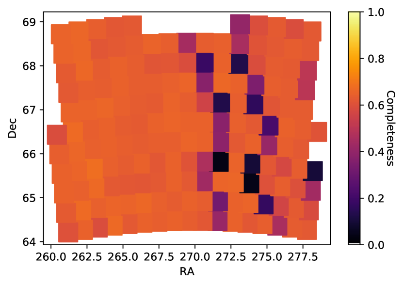
Figure 5: Completeness measures averaged over $\log L(\rm Ly\alpha$)=43.5–44.0 and $z=6.52$–6.62 for each skycell in HEROES.

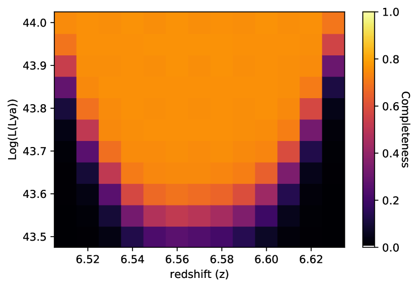
Figure 6: Completeness measures averaged over all skycells in HEROES.

6 Luminosity Functions

We calculate the comoving survey volume from the FWHM bounds of the NB921 filter in redshift space ($z=6.52$–6.62) and from the 30 deg² NEP survey area. We find a comoving volume of $2.46\times 10^{7}$ Mpc³. For the 4 deg² COSMOS field (Hu et al., 2016), we find a comoving volume of $3.28\times 10^{6}$ Mpc³. The combined comoving volume is then $2.78\times 10^{7}$ Mpc³.

We use this volume to construct the $z=6.6$ ULLAE LF at $\log L($Ly$\alpha$)$>43.5$ erg s^-1. Since all of our sources are spectroscopically observed and have reliable spectroscopic redshifts, the filter transmission profile corrections are exact in the determinations of the source luminosities. Additionally, we do not need to correct for contaminating sources, such as lower-redshift [OIII] emitters or high-redshift AGNs, as would be necessary in the analysis of purely photometric samples. We applied our incompleteness correction by dividing the uncorrected $\log\phi$ of each of the two luminosity bins ($\log L(\textrm{Ly$\alpha$})=43.5-43.75$ and $43.75-44\textrm{ erg s}^{-1}$) by the overall completeness in each bin. In Table 3, we give our incompleteness corrected and uncorrected LF measurements for the two $\Delta\log L(\textrm{Ly$\alpha$})=0.25$ bins, as well as the completeness of each bin. Our uncertainties are purely Poissonian.

Table 3: Luminosity Function Data

$\log L(\textrm{Ly$\alpha$})$	Uncorrected $\log\phi$	Corrected $\log\phi$	Completeness
	[$\Delta\log L(\textrm{Ly$\alpha$})]^{-1}$ Mpc-3	[$\Delta\log L(\textrm{Ly$\alpha$})]^{-1}$ Mpc-3
$43.625$	$-5.940^{+0.131}_{-0.198}$	$-5.526^{+0.131}_{-0.198}$	0.385
$43.875$	$-6.365^{+0.189}_{-0.374}$	$-6.198^{+0.189}_{-0.374}$	0.680

Note. — LF measurements for bin widths of $\Delta\log L(\textrm{Ly$\alpha$})=0.25$. The uncertainties are Poissonian.

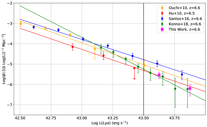
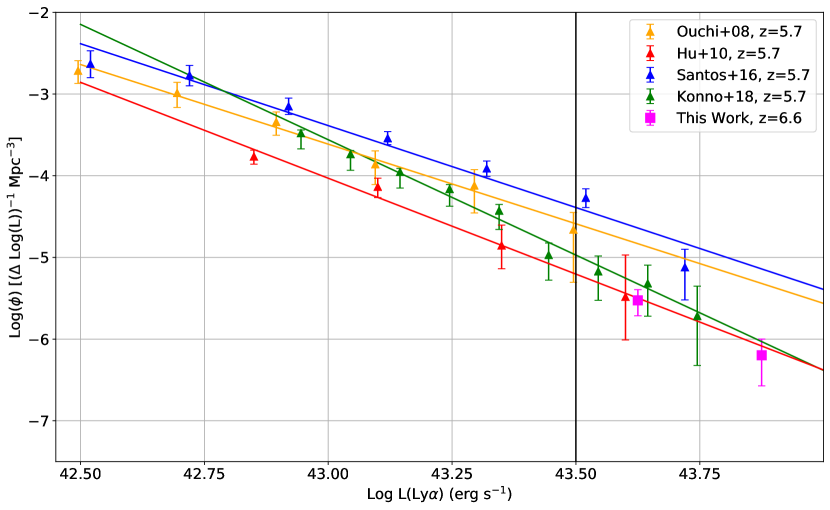
Figure 7: LF measurements for our $z=6.6$ ULLAE sample, divided into two bins (pink squares): $43.5~{}{\rm erg~{}s}^{-1}<\log L(\rm Ly\alpha)<43.75$ erg s^-1 and $43.75~{}{\rm erg~{}s}^{-1}<\log L(\rm Ly\alpha)<44.0$ erg s^-1. The vertical line defines our ultraluminous cutoff at $\log L(\rm Ly\alpha)>43.5$ erg s^-1. For comparison, we plot literature LAE LFs at (a) $z=6.6$ (Ouchi et al., 2010; Hu et al., 2010; Santos et al., 2016; Konno et al., 2018) and (b) $z=5.7$ (Ouchi et al., 2008; Hu et al., 2010; Santos et al., 2016; Konno et al., 2018) (see legends for colors). Note that the $z=6.6$ LF of Santos et al. (2016) is an updated version from Matthee et al. (2015). All the literature samples at both redshifts are well represented by individual power law fits (matching colored lines).

In Figure 7, we show these measurements as pink squares, along with various (a) $z=6.6$ and (b) $z=5.7$ LAE LFs from the literature, for comparison (see figure legend for colors). For each individual literature sample, we overlay power law fits using free indices and normalizations (matching colored lines). The LF from Konno et al. (2018) differs strikingly in shape from the remainder, perhaps indicating a problem with the methodology of using a primarily photometric sample from the HSC SSP. Excluding Konno et al. (2018), the remaining analyses are in fair agreement over the power law index.

Although it is common in the literature to fit Schechter functions, it is readily apparent from Figure 7 that the power law fits are a good representation of the data. The lack of an abrupt fall-off suggests we have not yet reached $L_{\ast}$. Since single power law fits cannot go on indefinitely, ultimately the LFs will have to turn down. This may occur at luminosities just slightly higher than the present ones.

The main point to take away from Figure 7 is that none of the LFs from the literature are fully consistent in both power law index and normalization with any of the others. Thus, for a proper evaluation of whether there is evolution of the LF with redshift, it is clear that the samples at the two redshifts need to be collected and analyzed in exactly the same way.

In our case, this means we can compare with the spectroscopically confirmed $z=6.6$ and $z=5.7$ LAE LFs of Hu et al. (2010), though they only have one ultraluminous point at $z=5.7$, and it has large uncertainties. Indeed, our $z=6.6$ ULLAE LF matches very well to both of their LFs. This would suggest that there is no evolution in the LFs at the ultraluminous end over this redshift range. However, we need more spectroscopically confirmed ULLAEs at $z=5.7$ to make a definitive statement.

For ease of comparison, we show in Figure 7 the various LFs for a fixed power law index of $-2$ and logarithmic normalization of 82.0544 in units of $[\Delta\log L(\textrm{Ly$\alpha$})]^{-1}$ Mpc^-3, taken from the best fit to Ouchi et al. (2010) assuming a fixed power law index of $-2$. This time we also separate them into four panels, each of which contains the $z=5.7$ and $z=6.6$ LAE LFs from a single group, along with our $z=6.6$ ULLAE LF (pink squares) for comparison.

In the first panel, we show the LFs of Ouchi et al. (2008) and Ouchi et al. (2010). They do not have any data at the ultraluminous end, so we cannot make a direct comparison with our ULLAE LF. They claim a decrease from $z=5.7$ to $z=6.6$ at the $>90$% confidence level at the lower luminosity end, with the $z=6.6$ luminosity density about 30% of the $z=5.7$ luminosity density.

In the second panel, we show the LFs of Hu et al. (2010) where, as we noted above, we are in agreement with their single $z=5.7$ point at the ultraluminous end (suggesting no evolution), though their point has large uncertainties. In their LF comparison, they found a multiplicative factor of two decrease in the number density of LAEs from $z=5.7$ to $z=6.5$.

In the third panel, we show the LFs of Santos et al. (2016). They have several data points at both redshifts at the ultraluminous end, but their LFs are 0.3–0.6 dex higher than ours. Konno et al. (2018) also noted that the Santos et al. (2016) number densities of LAEs at all luminosities were too high. Santos et al. (2016) (and previously Matthee et al. 2015 at $z=6.6$) studied the COSMOS, UDS, and SA22 fields with Suprime-Cam using a primarily photometric sample. Thus, the differences in normalization could be due to their assumptions about the redshifts in making the filter transmission profile corrections, flux systematics, and/or the presence of contaminants that are inherently absent in our spectroscopically confirmed sample. They find no evolution in the number density at the ultraluminous end from $z=5.7$ to $z=6.6$, but they see a significant decline at the lower luminosity end (by $0.5\pm 0.1$ dex). This drop is similar to that seen by Ouchi et al. (2008) and Ouchi et al. (2010) and by Hu et al. (2010).

Finally, in the fourth panel, we show the LFs of Konno et al. (2018). Their shape inconsistencies with the other surveys are strongly apparent in this figure. They have multiple data points at both redshifts at the ultraluminous end (though with significant uncertainties), and we find good agreement with their $z=6.6$ measurements. Again, they see evidence for a decrease at the lower luminosity end from $z=5.7$ to $z=6.6$ at the $>90$% confidence level. The evolution they derive is similar to that reported by the other groups. They make no claim about the evolution of the LFs at the ultraluminous end.

As discussed above, given the discrepancies between the different groups’ LFs, one needs to exercise caution in making claims about the evolution of the LAE LF from $z=5.7$ to $z=6.6$ unless one is comparing samples taken and analyzed in exactly the same way. For us, this means we can make comparisons with the Hu et al. (2010) samples at both redshifts; however, they are primarily at non-ULLAE luminosities. In future work, we plan to follow up spectroscopically a population of $z=5.7$ ULLAE candidates selected from HEROES in order to construct the LF at the ultraluminous end. Then we will be able to make direct comparisons with the spectroscopically confirmed $z=6.6$ ULLAE sample presented in this paper, and hence determine with our own data set whether there is any evolution from $z=5.7$ to $z=6.6$ at the ultraluminous end.

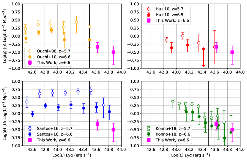
Figure 8: Evolution of the Ly$\alpha$ LF from $z=5.7$ to $z=6.6$ for four different surveys, all shown relative to our $z=6.6$ ULLAE LF (pink squares). Minute shifts of $\pm 0.02$ in $\log L(\rm Ly\alpha)$ have been made to avoid overlap of the data points.

7 Summary

The primary results from our work are as follows:

• Using 30 deg² of deep Subaru HSC $g^{\prime}$, $r^{\prime}$, $i^{\prime}$, $z^{\prime}$, and NB921 imaging of the NEP field, we identified 14 $z=6.6$ ULLAE candidates.

• We spectroscopically observed with Keck DEIMOS 7 of the candidates, and the remaining 7 were previously observed by Songaila et al. (2018). This provides 9 apectroscopically confirmed $z=6.6$ ULLAEs in the NEP field.

• We supplemented the 9 NEP ULLAEs with two spectroscopically confirmed $z=6.6$ ULLAEs in the COSMOS field for a total sample of 11. After applying corrections for the narrowband filter transmission profile and incompleteness, we constructed the $z=6.6$ ULLAE LF from this sample.

• We compared our $z=6.6$ ULLAE LF with $z=5.7$ and $z=6.6$ LAE LFs from the literature. We showed that none of the literature LFs are fully consistent in both power law index and normalization with any of the others, with the Santos et al. (2016) LFs, in particular, being too high, and the Konno et al. (2018) LFs having an odd shape.

• Given the variations in the literature LFs, it is clear that to determine the evolution of the LAE LF from $z=5.7$ to $z=6.6$, one should only compare LFs at the two redshifts that have been constructed in exactly the same way. We therefore compared our $z=6.6$ ULLAE LF with the $z=5.7$ and $z=6.6$ LAE LFs of Hu et al. (2010), which are also spectroscopically confirmed. We found that ours matched very well to both of theirs, suggesting no evolution in the LFs at the ultraluminous end.

• However, Hu et al. (2010) only have one ultraluminous point at $z=5.7$, and it has large uncertainties. Thus, we are working on a spectroscopically complete ULLAE LF analysis at $z=5.7$ that should allow us to determine within our own data set whether the ULLAE LF evolves over this redshift range.

8 Acknowledgments

We thank the anonymous referee for a constructive report that helped us to improve this paper. We gratefully acknowledge support for this research from Jeff and Judy Diermeier through a Diermeier Fellowship (A.J.T.), NSF grants AST-1716093 (E.M.H., A.S.) and AST-1715145 (A.J.B), the trustees of the William F. Vilas Estate (A.J.B.), and the University of Wisconsin-Madison, Office of the Vice Chancellor for Research and Graduate Education with funding from the Wisconsin Alumni Research Foundation (A.J.B.).

This paper is based in part on data collected from the Subaru Telescope. The Hyper Suprime-Cam (HSC) collaboration includes the astronomical communities of Japan and Taiwan, and Princeton University. The HSC instrumentation and software were developed by the National Astronomical Observatory of Japan (NAOJ), the Kavli Institute for the Physics and Mathematics of the Universe (Kavli IPMU), the University of Tokyo, the High Energy Accelerator Research Organization (KEK), the Academia Sinica Institute for Astronomy and Astrophysics in Taiwan (ASIAA), and Princeton University. Funding was contributed by the FIRST program from Japanese Cabinet Office, the Ministry of Education, Culture, Sports, Science and Technology (MEXT), the Japan Society for the Promotion of Science (JSPS), Japan Science and Technology Agency (JST), the Toray Science Foundation, NAOJ, Kavli IPMU, KEK, ASIAA, and Princeton University. The NB921 filter was supported by KAKENHI (23244025) Grant-in-Aid for Scientific Research (A) through the Japan Society for the Promotion of Science (JSPS).

This paper also makes use of data collected at the Subaru Telescope and retrieved from the HSC data archive system, which is operated by Subaru Telescope and Astronomy Data Center at National Astronomical Observatory of Japan. Data analysis was in part carried out with the cooperation of Center for Computational Astrophysics, National Astronomical Observatory of Japan.

This paper is based in part on data collected from the Keck II Telescope. The W. M. Keck Observatory is operated as a scientific partnership among the California Institute of Technology, the University of California, and NASA, and was made possible by the generous financial support of the W. M. Keck Foundation.

The authors wish to recognize and acknowledge the very significant cultural role and reverence that the summit of Maunakea has always had within the indigenous Hawaiian community. We are most fortunate to have the opportunity to conduct observations from this mountain.

References

- Aihara et al. (2019) Aihara, H., AlSayyad, Y., Ando, M., et al. 2019, PASJ, 71, 114
- Bertin & Arnouts (1996) Bertin, E., & Arnouts, S. 1996, A&AS, 117, 393
- Cowie et al. (1996) Cowie, L. L., Songaila, A., Hu, E. M., & Cohen, J. G. 1996, AJ, 112, 839
- Hu et al. (2010) Hu, E. M., Cowie, L. L., Barger, A. J., et al. 2010, ApJ, 725, 394
- Hu et al. (2004) Hu, E. M., Cowie, L. L., Capak, P., et al. 2004, AJ, 127, 563
- Hu et al. (1998) Hu, E. M., Cowie, L. L., & McMahon, R. G. 1998, ApJ, 502, L99
- Hu et al. (2016) Hu, E. M., Cowie, L. L., Songaila, A., et al. 2016, ApJ, 825, L7
- Hu et al. (2019) Hu, W., Wang, J., Zheng, Z.-Y., et al. 2019, ApJ, 886, 90
- Itoh et al. (2018) Itoh, R., Ouchi, M., Zhang, H., et al. 2018, ApJ, 867, 46
- Jiang et al. (2017) Jiang, L., Shen, Y., Bian, F., et al. 2017, ApJ, 846, 134
- Kashikawa et al. (2011) Kashikawa, N., Shimasaku, K., Matsuda, Y., et al. 2011, ApJ, 734, 119
- Konno et al. (2014) Konno, A., Ouchi, M., Ono, Y., et al. 2014, ApJ, 797, 16
- Konno et al. (2018) Konno, A., Ouchi, M., Shibuya, T., et al. 2018, PASJ, 70, S16
- Magnier et al. (2016) Magnier, E. A., Schlafly, E. F., Finkbeiner, D. P., et al. 2016, arXiv e-prints, arXiv:1612.05242
- Matthee et al. (2020) Matthee, J., Sobral, D., Gronke, M., et al. 2020, MNRAS, 492, 1778
- Matthee et al. (2015) Matthee, J., Sobral, D., Santos, S., et al. 2015, MNRAS, 451, 400
- Matthee et al. (2019) Matthee, J., Sobral, D., Boogaard, L. A., et al. 2019, ApJ, 881, 124
- Ota et al. (2017) Ota, K., Iye, M., Kashikawa, N., et al. 2017, ApJ, 844, 85
- Ouchi et al. (2008) Ouchi, M., Shimasaku, K., Akiyama, M., et al. 2008, ApJS, 176, 301
- Ouchi et al. (2010) Ouchi, M., Shimasaku, K., Furusawa, H., et al. 2010, ApJ, 723, 869
- Santos et al. (2016) Santos, S., Sobral, D., & Matthee, J. 2016, MNRAS, 463, 1678
- Sobral et al. (2015) Sobral, D., Matthee, J., Darvish, B., et al. 2015, ApJ, 808, 139
- Songaila et al. (2018) Songaila, A., Hu, E. M., Barger, A. J., et al. 2018, ApJ, 859, 91
- Zheng et al. (2017) Zheng, Z.-Y., Wang, J., Rhoads, J., et al. 2017, ApJ, 842, L22