Non-Precipitating Shallow Cumulus Clouds: Theory and Direct Numerical Simulation

Abstract

We model cumulus clouds as transient diabatic plumes, and present a single-fluid formulation for the study of the dynamics of developing shallow cumulus clouds. The fluid, air, carries water vapour and liquid water as scalars that are advected with the flow. We employ the Boussinesq approximation and a simplified form of the Clausius-Clapeyron law for phase changes. We use this formulation to study the ambient conditions required for the formation of cumulus clouds. We show that the temperature lapse rate in the ambient, $\Gamma_{0}$; and the relative humidity of the ambient, $s_{\infty}$, are crucial in deciding when cumulus clouds form. In the phase-space of these two parameters, we determine the boundary that separates the regions where cumulus clouds can form and where they cannot.

I Introduction

Cumulus clouds, from the Latin for ‘heap’, can be of a wide range of sizes and take a variety of shapes. The classification of cloud types by the WMO (Cohn, 2017) recognises several species of cumulus clouds depending on shape, size and altitude. The common feature uniting these various types is that cumulus clouds are typically active; that is, they consist of strong updraughts driven by local sources of buoyancy, and have lifetimes that last only as long as the updraughts that feed them. Cumulus lifetimes can vary from less than an hour to a few hours.

Clouds are, in general, suspensions of liquid water droplets, and possibly ice particles as well, of various sizes in a mixture of air and water vapour (Cohn, 2017). Clouds play a crucial role in the planet’s climate, and are the last bastion of uncertainty in climate modelling, being responsible for significant feedback on both short-wave and long-wave radiation (Stevens and Bony, 2013; Bony et al., 2015). The response of this radiative feedback to surface conditions is the focus of climate research. This response depends on the amount of energy and the mass of water vapour that is transported from the surface to higher altitudes, and on the variation of these fluxes with changes in surface conditions. The transport of thermal energy and water vapour from the surface to higher altitudes occurs through the formation of clouds in the atmosphere.

As the atmosphere generally gets colder and lighter with increasing altitude, water vapour cools and condenses into liquid water droplets as it rises in the atmosphere. This change of phase releases a significant amount of energy into the flow, changing the nature of the flow. Clouds are thus not only markers of the patterns of flow in the atmosphere, but also regions where the flow in the atmosphere is qualitatively different from its surroundings. Because of the qualitative difference between ascending flow (with saturated vapour) and descending flow (with unsaturated vapour) in the atmosphere, convection in the atmosphere often takes the form of narrow strong upwelling regions (called hot towers) surrounded by broad regions of weak downward flow. This was first recognised by Bjerknes (1938). These tall towers of upward flow are thus responsible for the upward transport of mass and thermal energy in the atmosphere; these fluxes are controlled by the interaction of the cloud flow with the ambients. Hot towers are one common form of cumulus clouds, and their interaction with ambient fluid results in entrainment into or detrainment from the cloud flow.

The evolution of a cumulus cloud depends on surface and ambient conditions, including the surface temperature, the ambient temperature and its rate of decrease with height, the ambient aerosol content (amount, type, size distribution), and covers length scales from fractions of a micrometre (Pruppacher and Klett, 2010, Chapter 2) to the characteristic dimensions of the cloud—a few hundred metres in width, and up to several kilometres in height (Narasimha et al., 2011). The amount of liquid water (and solid ice in some cases), and the size distributions of the particles making up these phases, also vary over the lifetime of a cumulus cloud; water droplets of a sufficiently large size (typically about a millimetre; see Pruppacher and Klett (2010, Chapter 2)) fall out of the cloud as precipitation. Given the wide range of lengthscales and the variety of physical interactions invovled, a complete and accurate description of the evolution of a cloud is impossible, either through observations or through computer simulations (Grabowski and Wang, 2013; Randall et al., 2003). Simplified descriptions of the dynamics are thus required. These simplifications involve neglecting processes that are unimportant for certain types of cloud and/or during certain periods of the cloud’s lifetime.

In this paper, we study the fluid dynamics of a non-precipitating shallow cumulus cloud, modelled as an isolated turbulent plume from a finite source of buoyancy. Ignoring precipitation obviates the modelling of the suspended phase, which may then be treated as a scalar carried with the flow while retaining the thermodynamics of condensation and evaporation. Restricting ourselves to shallow clouds allows us to ignore compressibility effects and employ the Boussinesq equations of motion (Eq. 13).

The problem of entrainment in free-shear flows is of significant fluid mechanical interest, and has been the object of study for several decades (Morton et al., 1956; Turner, 1962). Cumulus clouds, being free-shear flows, are thus of interest in understanding this fundamental process in free-shear flows. In addition, as mentioned above, cumulus clouds and their interaction with their ambients are a crucial and as-yet poorly understood piece of the global climate puzzle. Most GCMs model cumulus clouds as steady plumes (De Rooy et al., 2013). This is inconsistent with well-known results that heated free-shear flows have anomalous entrainment (see, e.g., Bhat and Narasimha (1996)). A model for cumulus clouds incorporating the effects of anomalous entrainment is the transient diabatic (as opposed to adiabatic) plume, introduced in Narasimha et al. (2011) and shown to be able to reproduce commonly observed cloud shapes. It was also shown in the latter study that the Reynolds number, as long as it is large enough, is not a crucial parameter, an idea we will use repeatedly. We note in passing that shallow vigorous cumulus clouds may be modelled as bubbles/thermals; first introduced by Turner (1969), an idea that has become popular again (Lecoanet and Jeevanjee, 2019).

Convection in the atmosphere is also modelled as moist Rayleigh-Benard convection (Pauluis et al., 2010; Schumacher and Pauluis, 2010; Wu et al., 2009). We note that highly turbulent Rayleigh-Benard convection takes the form of penetrative plumes (Kadanoff, 2001; Puthenveettil and Arakeri, 2005), which are responsible for significant portions of the energy and mass transfer in the flow. The approach here studies, without the horizontal movement that normally occurs in a Rayleigh-Benard setup, a single plume and its interaction with its ambient. The modelling of cumulus clouds as isolated turbulent plumes is thus complemetary to the study of moist Rayleigh-Benard convection.

The rest of the paper is organised as follows. In §II, the nondimensional governing equations are written down and simplified, and these simplifications justified. In §III, the numerical algorithm used in our study is described. Results from the simulations are presented in §IV, and compared with those from a simple one-dimensional model (§IV.1) along the lines of Morton et al. (1956). We convert to scales typical of the atmosphere and comment on what the nondimensional solutions mean for clouds. We conclude in §V.

II Problem Setup

The dynamics of interest involves the rise of a plume, carrying water vapour, in a stratified ambient with a known relative humidity. When the vapour pressure is greater than the local saturation vapour pressure, it condenses into liquid water, heating the flow and increasing its buoyancy. A description of the flow thus needs to incorporate the dynamics of a turbulent plume in a stratified ambient along with the thermodynamics of phase-change of water, from vapour to liquid and vice-versa. It will be useful to begin by writing down the conventions used for naming variables and parameters.

II.1 Notation

The following conventions are used for all symbols.

• The vertical direction is $x$, and gravity points along $-\boldsymbol{e}_{x}$.

• Dimensional quantities are denoted by symbols with tilde ($\tilde{}$); the tilde is dropped once the variable is nondimensionalised.

• Symbols with a subscript infinity _∞ denote ambient quantities (usually functions of the height above ground level) away from, and not affected by, the flow.

• Quantities at ground level are given the subscript zero (₀).

• The water-substance mixing ratios (defined in eq. 8) are denoted with a hat ($\hat{}$) before they are normalised using a base value (see eq. 11).

• Combinations of the above are possible: the base temperature, for instance, is $T_{\infty,0}$ (eq. 1).

II.2 The stratified ambient

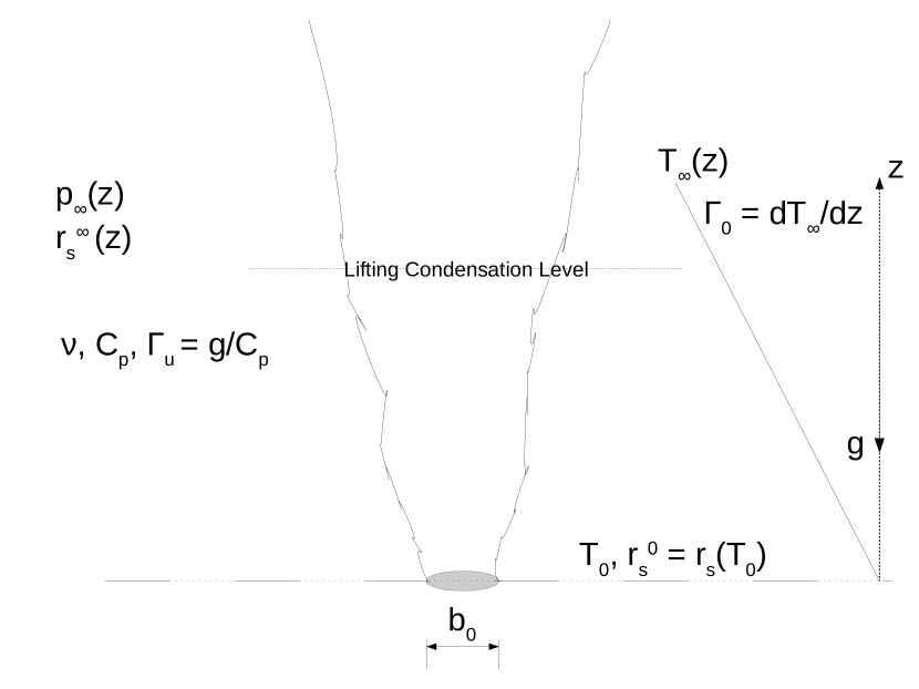
Figure 1: Schematic depiction of the system. The hot patch in grey is a source for both temperature and vapour.

The plume emanates from a circular patch on the ground of diameter $b_{0}$, which we will choose as the length-scale. This hot-patch has a temperature difference $\Delta T_{0}$ over the rest of the surface at $x=0$, which is at a temperature $T_{\infty,0}$. We will use $\Delta T_{0}$ as the scale for temperature differences. Together, $T_{\infty,0}$ and $\Delta T_{0}$ define the Atwood number $\epsilon=\Delta T_{0}/T_{\infty,0}$, which is typically $\mathcal{O}\left(10^{-2}\right)$. We will use the fact that this ratio is small in what follows. For the stratification to be stable, the density of the fluid must decrease with height above ground level. The strength of the stratification is given in terms of the rate of decrease of density with height; the larger the rate, the stabler the stratification.

In a dry gas, density and temperature are connected via the gas law $p_{\infty}\left(x\right)=\rho_{d,\infty}R_{d}T_{\infty}$, with $p_{\infty}\left(x\right)$ being the ambient pressure at a height $x$ above ground-level, $\rho_{d,\infty}$ the density of dry air, and $R_{d}$ the gas constant for dry air. The stratification may thus be prescribed in terms the ambient temperature $T_{\infty}\left(x\right)$ which decreases linearly with height:

$$T_{\infty}\left(x\right)=T_{\infty,0}-\tilde{\Gamma}_{0}x,$$ (1)

where $T_{\infty,0}=T_{\infty}\left(0\right)$. For a shallow cloud, the ambient temperature may be assumed to vary linearly with height; and the lapse rate, i.e. the rate at which the ambient temperature falls with height, is

$$\tilde{\Gamma}_{\infty}\left(x\right)=-\frac{dT_{\infty}}{dx}=\tilde{\Gamma}_{0}=\text{const}.$$

A dry atmosphere with no radiative effects composed of a single gas has a dry (subscript _d) adiabatic lapse rate $\tilde{\Gamma}_{d}=g/C_{p}$, where $g$ is the acceleration due to gravity and $C_{p}$ is the specific heat of the gas at constant pressure. The actual lapse rate $\tilde{\Gamma}_{0}$ (which is in general different from $\tilde{\Gamma}_{d}$) must be considered in comparison to the dry adiabatic lapse rate. For dry convection, ambient conditions are stably, neutrally or unstably stratified accordingly as $\tilde{\Gamma}_{0}\lesseqqgtr\tilde{\Gamma}_{d}$ (see, e.g. Pauluis et al. (2010)). The lapse rates $\tilde{\Gamma}_{d}$ and $\tilde{\Gamma}_{0}$ are nondimensionalised using $\Delta T_{0}$ and $b_{0}$:

$$\Gamma_{d} =\frac{\tilde{\Gamma}_{d}b_{0}}{\Delta T_{0}}=\frac{\tilde{\Gamma}_{d}b_{0}}{T_{\infty,0}\epsilon},$$

$$\Gamma_{0} =\frac{\tilde{\Gamma}_{0}b_{0}}{\Delta T_{0}}=\frac{\tilde{\Gamma}_{0}b_{0}}{T_{\infty,0}\epsilon}.$$

We will report our results in terms of the above nondimensional lapse-rates.

The pressure $p_{\infty}\left(x\right)$ in the ambient is given by

$$\frac{p_{\infty}\left(x\right)}{p_{\infty,0}}=\left(\frac{T_{\infty}\left(x\right)}{T_{\infty,0}}\right)^{g/\tilde{\Gamma}_{0}R_{d}}.$$ (2)

In making the Boussinesq approximation for shallow clouds (discussed in section II.4), we set this ratio to unity, and therefore assume that $p_{\infty}\left(x\right)=p_{\infty,0}$.

The buoyancy $B$ of a cloud parcel is given by the density difference between the parcel and the ambient. The density of a parcel containing both vapour and liquid water components is

$$\rho=\rho_{d}\left(1+\tilde{r}_{v}+\tilde{r}_{l}\right),$$

which is a reasonable assumption when $\tilde{r}_{v},\tilde{r}_{l}\ll 1$. The density of the ambient, with the background mixing ratio $\tilde{r}_{v,\infty}$ of vapour, is similarly given by

$$\rho_{\infty}=\rho_{d,\infty}\left(1+\tilde{r}_{v,\infty}\right).$$

In open flows such as we have, the thermodynamic pressure inside the cloud can be assumed to be the same as the ambient pressure. We thus have for the ambient

$$p_{\infty}=p_{d,\infty}+p_{v,\infty}=\rho_{d,\infty}\left(1+\frac{R_{v}}{R_{d}}\tilde{r}_{v,\infty}\right)R_{d}T_{\infty}=\rho_{d,\infty}\left(1+\chi\tilde{r}_{v,\infty}\right)R_{d}T_{\infty},$$

where $\chi$ is the ratio of the gas constants of air and water, $\chi=R_{v}/R_{d}=28.9/18=1.61.$ Similarly, for a cloud parcel,

$$p_{\infty} =\rho_{d}R_{d}\left(1+\frac{R_{v}}{R_{d}}\tilde{r}_{v}\right)T.$$

Thus, the ratio of densities is

$$\frac{\rho}{\rho_{\infty}} =\frac{\rho_{d}\left(1+\tilde{r}_{v}+\tilde{r}_{l}\right)}{\rho_{d,\infty}\left(1+\tilde{r}_{v,\infty}\right)}=\left(\frac{T_{\infty}}{T}\right)\left(\frac{1+\chi\tilde{r}_{v,\infty}}{1+\chi\tilde{r}_{v}}\right)\left(\frac{1+\tilde{r}_{v}+\tilde{r}_{l}}{1+\tilde{r}_{v,\infty}}\right)$$

$$=\frac{T_{\infty}}{T}\left[1+\left(\chi-1\right)\left(\tilde{r}_{v,\infty}-\tilde{r}_{v}\right)+\tilde{r}_{l}\right]$$

$$=\frac{T_{\infty}}{T}+\frac{T_{\infty}}{T}\left[\left(\chi-1\right)\left(\tilde{r}_{v,\infty}-\tilde{r}_{v}\right)+\tilde{r}_{l}\right].$$

It follows that

$$1-\frac{\rho}{\rho_{\infty}} =1-\frac{T_{\infty}}{T}-\frac{T_{\infty}}{T}\left[\left(\chi-1\right)\left(\tilde{r}_{v,\infty}-\tilde{r}_{v}\right)+\tilde{r}_{l}\right]$$

$$\approx\frac{T-T_{\infty}}{T_{\infty}}-\left(\left(\chi-1\right)\left(\tilde{r}_{v,\infty}-\tilde{r}_{v}\right)+\tilde{r}_{l}\right),$$

where we have taken $T/T_{\infty}\approx 1$ in the second term and replaced the denominator $T$ in the first term with $T_{\infty}$. We then have, for the buoyancy,

$$B=g\frac{\rho_{\infty}-\rho}{\rho_{\infty}}=g\left[\frac{T-T_{\infty}}{T}+\left(\chi-1\right)\left(\tilde{r}_{v}-\tilde{r}_{v,\infty}\right)-\tilde{r}_{l}\right].$$ (3)

If we assume that temperature differences are $\mathcal{O}\left(\Delta T\right)$, the buoyancy $B=\mathcal{O}\left(g\epsilon\right)$. The velocity scale in the problem has to be derived from the a priori assumption that the buoyancy forces in the problem are $\mathcal{O}\left(1\right)$ compared to the advective forces. That is,

$$Fr^{2}=\frac{W^{2}/b_{0}}{g\epsilon}=\mathcal{O}(1),$$ (4)

giving, for the velocity scale,

$$W=\sqrt{b_{0}g\epsilon}.$$ (5)

We work with absolute temperatures (instead of potential temperatures as is more common in the atmospheric sciences). Temperature differences are scaled in units of $\Delta T_{0}$, giving the nondimensional temperature differential.

$$\theta=\frac{T-T_{\infty}\left(x\right)}{\Delta T_{0}}.$$ (6)

We will assume that $\nu$ the kinematic viscosity of the fluid is also known and constant. Together with the length and velocity scales defined above, this defines the Reynolds number

$$Re=\frac{Wb_{0}}{\nu}=\frac{b_{0}\sqrt{b_{0}g\epsilon}}{\nu}.$$ (7)

The Prandtl number $Pr=\nu/\kappa$, the ratio between the diffusivities of momentum and temperature, is $\mathcal{O}\left(1\right)$ for gases. For simplicity, we take $Pr=1$.

II.3 Thermodynamics

Cloud flows are complicated by the addition of the thermodynamics of phase-change to the dynamics of plumes in stratified ambients. The amounts of water vapour and liquid water present are given in terms of the mixing ratios of vapour (subscript _v) and liquid (subscript _l) respectively. These are defined as the mass of water substance per unit mass of dry air. For instance, the mixing ratio of vapour is

$$\hat{r}_{v}=\frac{\rho_{v}}{\rho_{d}}.$$ (8)

The thermodynamics of water is governed by the Clausius-Clapeyron law which gives the saturation mixing ratio of vapour at a temperature $T$ and pressure $p_{\infty}\left(x\right)$, and can be written as

$$\hat{r}_{s}\left(T,p_{\infty}\left(x\right)\right)=r_{s,0}\frac{p_{\infty,0}}{p_{\infty}\left(x\right)}\mbox{exp}\left(\frac{L_{v}}{R_{V}}\left(\frac{1}{T_{\infty,0}}-\frac{1}{T}\right)\right),$$ (9)

where $r_{s,0}$ is the saturation mixing ratio at the ground-level temperature and pressure $\left(T_{\infty,0},p_{\infty,0}\right)$. In addition, $L_{v}$ is the latent heat of vapourisation of water, and $R_{v}$ is the gas constant for water vapour. We assume that the ambient has a background concentration of water vapour, given by

$$\hat{r}_{v}^{\infty}=s_{\infty}\left(x\right)\times\hat{r}_{s}\left(T_{\infty}(x),p_{\infty}(x)\right),$$ (10)

with $s_{\infty}\left(x\right)$ being the relative humidity of the ambient which can be a function of altitude. The corresponding background concentration of liquid water is $\hat{r}_{l}^{\infty}=0$.

We will make a few simplifying assumptions. First, in defining the mixing ratio $\hat{r}_{l}$ for liquid water in the flow, we ignore the details of the size-distribution of the water droplets that make up the liquid water. Called the one-moment scheme in atmospheric physics, this is justifiable for non-precipitating clouds (see, e.g. Morrison et al. (2009)). We will also assume that the liquid field thus defined is advected with the flow, also justifiable if the liquid content is made up of a very large number of small droplets. This is again true for non-precipitating clouds, in which the size-distribution of the droplets peaks at around $10\mu$m.

We will also, henceforth, scale all mixing ratios in units of the saturation mixing ratio $r_{s,0}\left(T_{\infty,0},p_{\infty,0}\right)$ at the ground-level, and denote these scaled mixing ratios by dropping the $\hat{}$. Thus, in these scaled units, eq. 9 becomes

$$r_{s}\left(T,p_{\infty}\left(x\right)\right)=\frac{\mbox{exp}\left(\frac{L_{v}}{R_{V}}\left(\frac{1}{T_{\infty,0}}-\frac{1}{T}\right)\right)}{p_{\infty}\left(x\right)/p_{\infty,0}}.$$ (11)

In addition, we assume that the species Prandtl numbers associated with vapour and liquid diffusivities, denoted by $Pr_{v}$ and $Pr_{l}$ respectively, are both unity. This is a reasonable assumption for the vapour. Liquid droplets in evolving cumulus clouds have a size distribution that peaks around $10\mu$m (Pruppacher and Klett, 2010), and are therefore not influenced by Brownian diffusion. As a first approximation, however, we proceed with this assumption. Small-scale features of the flow will, as a result, be affected.

II.3.1 Supersaturation and thermodynamics of phase-change

We assume, further, that mixtures of air and water vapour can be supersaturated; i.e. that more vapour than prescribed by the Clausius-Clapeyron law (eq. 9) can exist in a parcel of a given temperature. In such supersaturated parcels, the water vapour condenses into liquid water at a rate which depends on the supersaturation:

$$\frac{dr_{v}}{dt}\sim\left(\frac{r_{v}}{r_{s}}-1\right),$$

where the term on the right hand side is called the supersaturation. The supersaturation in atmospheric clouds is typically of the order of a few percent. The constant of proportionality in this equation is a timescale $\tilde{\tau}_{s}$, which can be derived by assuming the droplet number and distribution (see, e.g., Kumar et al. (2014)). This timescale is strictly a function of time and space, and its variation can affect the flow. However, if the droplet size distribution is monodisperse, and we consider only non-precipitating clouds, $\tau_{s}$ is typically small compared to the timescale $b_{0}/W$ of the flow. In this work, we choose a small value for

$$\tau_{s}=\frac{\tilde{\tau}_{s}W}{b_{0}}=0.1,$$

and do not discuss the effects of its variations. Thus, the rate of phase-change (in nondimensional variables) is given by

$$\frac{dr_{l}}{dt}=-\frac{dr_{v}}{dt}=\mathcal{H}\frac{1}{\tau_{s}}\left(\frac{r_{v}}{r_{s}}-1\right),$$ (12)

where $\mathcal{H}$ is a modified heaviside function, which is positive if the parcel is supersaturated, or if the parcel is subsaturated but has nonzero liquid content:

$$\mathcal{H}=\begin{cases}1&\text{if }r_{v}>r_{s}\\ 1&\text{if }r_{v}<r_{s}\text{ and }r_{l}>0\\ 0&\text{if }r_{v}<r_{s}\text{ and }r_{l}=0.\end{cases}$$

II.4 Boussinesq Approximation

II.4.1 Dynamics

The Boussinesq approximation involves assuming that flow is incompressible, even if the ambient is stratified (Spiegel and Veronis, 1960). The incompressibility condition is the shallow-convection limit of anelastic schemes that filter out the acoustic modes, so that the bound on the timestep to be used for numerical integration is relaxed considerably (see, e.g. Bannon (1996); Durran (1989)).

The Boussinesq approximation is only valid for clouds whose height is small compared to the density scale height

$$H_{\rho}=\left(\frac{1}{\rho}\frac{d\rho}{dx}\right)^{-1}$$

of the atmosphere. This height is typically $\mathcal{O}\left(10-15\text{ km}\right)$ (Bannon, 1996). We are therefore restricted to clouds which do not rise more than a few kilometres (see, e.g., Bannon (1996); Pauluis et al. (2010)).

II.4.2 Thermodynamics

In order to be consistent in our approximation, we also write the Clausius-Clapeyron law (eq. 9) using the Boussinesq approximation. This has the added benefit of letting us describe the problem independently of the absolute temperature $T_{\infty,0}$. First, we will find it convenient to define the nondimensional constants

$$L_{1} =\frac{L_{v}\epsilon}{R_{v}T_{\infty,0}}\text{ and}$$

$$L_{2} =\frac{L_{v}r_{s,0}}{C_{p}T_{\infty,0}\epsilon}.$$

The first of these quantities appears in the Clausius-Clapeyron equation 9 above. The second appears in the temperature equation. The two quantities are proportional to each other:

$$L_{1}=\left(\frac{C_{p}}{R_{v}}\right)\cdot\left(\frac{\epsilon}{r_{s,0}}\right)\cdot L_{2}.$$

Using $L_{1}$, we rewrite the Clausius-Clapeyron equation as follows. We take

$$\frac{1}{T_{\infty,0}}-\frac{1}{T} =\frac{\Delta T_{0}\theta-\tilde{\Gamma}_{0}\tilde{x}}{T_{\infty,0}\left(T_{\infty,0}-\Gamma_{0}x+\Delta T_{0}\theta\right)}$$

$$=\frac{1}{T_{\infty,0}}\left(\frac{\Delta T_{0}\theta-\tilde{\Gamma}_{0}\tilde{x}}{T_{\infty,0}-\Delta T_{0}\Gamma_{0}x+\Delta T_{0}\theta}\right)$$

$$=\frac{\epsilon}{T_{\infty,0}}\left(\frac{\theta-\Gamma_{0}x}{1-\epsilon\left(\Gamma_{0}x+\theta\right)}\right)\approx\frac{\epsilon}{T_{\infty,0}}\left(\frac{\theta-\Gamma_{0}x}{1-\epsilon\Gamma_{0}x}\right)$$

$$=\epsilon\frac{C(x)}{T_{\infty,0}}\left(\theta-\Gamma_{0}x\right),$$

where

$$C(x)=\frac{1}{1-\epsilon\Gamma_{0}x}=\frac{T_{\infty,0}}{T_{\infty}\left(x\right)}>1$$ (13)

is a nondimensional factor which is a function of the altitude. In the Boussinesq approximation, we set $C=1$ and the Clausius-Clapeyron law (Eq. 11) becomes

$$r_{s}=\text{exp}\left(-L_{1}\Gamma_{0}x\right)\text{exp}\left(L_{1}\theta\right)$$ (14)

The above equation does not depend directly on $T_{\infty,0}$; as a result, the results here can be directly applied to an arbitrary fluid as long as the correct values for $L_{1}$ and $L_{2}$ are specified.

The buoyancy term in the momentum equation has to be carefully approximated as well. As in §II.2, the contribution from temperature differences is

$$B\propto g\frac{T-T_{\infty}\left(x\right)}{T_{\infty}\left(x\right)},$$

which can be written in our nondimensional variables as

$$B\propto\frac{1}{Fr^{2}}\left(C(x)\cdot\theta\right),$$

where the approximation factor $C(x)=1/\left(1-\epsilon\Gamma_{0}x\right)$ appears again. As before, under the Boussinesq approximation, $C=1$, and the total buoyancy is

$$B=\frac{1}{Fr^{2}}\left(\theta+r_{0}\left(\left(\chi-1\right)\left(r_{v}-r_{v}^{\infty}\right)-r_{l}\right)\right),$$ (15)

(see, e.g. Hernandez-Duenas et al. (2013); Kumar et al. (2014)).

II.4.3 Validity of the Boussinesq approximation

As mentioned above, the factor $C(x)=\left(1-\epsilon\Gamma_{0}x\right)^{-1}>1$ for a lapsing atmosphere, and the Boussinesq approximation amounts to setting $C=1$. If the maximum altitude is not too large—i.e. if the cloud is shallow—the approximation $C\approx 1$ is a good one. The approximation becomes worse with increasing height. This can be seen in Figure 2, where the saturation mixing ratio $r_{s,\infty}\left(x\right)$ is plotted with and without the Boussinesq approximation $C(x)=1$. The ratio of the two is also plotted. The approximation $C=1$ occurs in two places: in the buoyancy term and in the saturation vapour mixing ratio term. In the buoyancy term, using the approximation $C=1$ results in an underestimation of the buoyancy. In the saturation mixing ratio term, setting $C=1$ underestimates the saturation mixing ratio, and thus overestimates whether a given mixing ratio of vapour at a given temperature is saturated.

The maximum value of the factor $C(x)$ occurs when $\Gamma_{0}$ is highest, and at the maximum $x$ of the computational domain. The maximum value of $\Gamma_{0}$ in our simulations is $\Gamma_{0}=0.09$. For this case, the maximum value of $C(x)=(1-0.09)^{-1}\approx 1.1$.

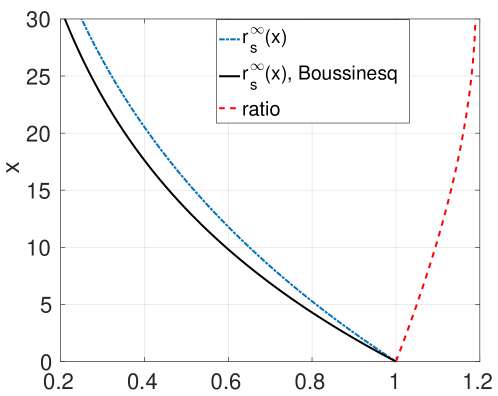
Figure 2: Validity of the Boussinesq approximation $C(x)=1$.

II.5 Nondimensional equations and boundary conditions

The continuity equation, in the Boussinesq approximation, is just the requirement that the divergence of the velocity be zero:

$$\nabla\cdot\mathbf{u}=0.$$ (16)

In writing Eq. 16, we are neglecting the changes in volume introduced by the condensation of water vapour. This is an approximation, valid only in the limit as $r_{v,l}\ll 1$.

The momentum equation has contributions from the buoyancy term discussed in §II.4, and reads

$$\frac{D\mathbf{u}}{Dt}=-\frac{\nabla p}{\rho_{0}}+\frac{1}{Fr^{2}}\left[\theta+r^{0}\left(\left(\chi-1\right)\left(r_{v}-r_{v}^{\infty}\right)-r_{l}\right)\right]\mathbf{e}_{x}+\frac{1}{Re}\nabla^{2}\mathbf{u},$$ (17)

where $D/Dt$ is the material derivative. The factor $L_{2}$ appears in the temperature equation as follows

$$\frac{D\theta}{Dt} =\left(\frac{\tilde{\Gamma}_{0}-\tilde{\Gamma}_{d}}{\Delta T_{0}}\right)\tilde{w}+\mathcal{H}\left(\frac{L_{v}r_{s,0}}{C_{p}\Delta T_{0}}\right)\left(\frac{1}{\tilde{\tau}_{s}}\right)\left(\frac{r_{v}}{r_{s}}-1\right)+\frac{1}{Re\cdot Pr}\nabla^{2}\theta,$$

which can be nondimensionalised to

$$\frac{D\theta}{Dt}=\left(\Gamma_{0}-\Gamma_{d}\right)w+L_{2}\left[\frac{\mathcal{H}}{\tau_{s}}\left(\frac{r_{v}}{r_{s}}-1\right)\right]+\frac{1}{Re\cdot Pr}\nabla^{2}\theta.$$ (18)

The vapour and liquid transport equations include the phase-change terms (eq. 12) and the diffusion terms discussed in §II.3:

$$\frac{Dr_{v}}{Dt}=-\left[\frac{\mathcal{H}}{\tau_{s}}\left(\frac{r_{v}}{r_{s}}-1\right)\right]+\frac{1}{Re\cdot Pr_{v}}\nabla^{2}r_{v},$$ (19)

$$\frac{Dr_{l}}{Dt}=\left[\frac{\mathcal{H}}{\tau_{s}}\left(\frac{r_{v}}{r_{s}}-1\right)\right]+\frac{1}{Re\cdot Pr_{l}}\nabla^{2}r_{l}.$$ (20)

These equations are similar to the non-equilibrium, non-precipitating equations proposed as a ‘minimal model’ for moist convection by Hernandez-Duenas et al. (2012). The major differences between their (non-equilibrium, non-precipitating) model and ours are that (a) they use the potential temperature since they deal with altitudes of up to $15$ km; and (b) they simplify the thermodynamics such that the saturation vapour pressure is only a function of the altitude above ground; (c) that their ambients are always nearly saturated. The first of these assumptions (i.e. the use of the potential temperature) may be relaxed if convection is shallow, as described in §II.5.1 above. Study of the details of the flow of vapour and liquid water, as we aim to do, requires local variations of saturation vapour pressure to be accounted for. Lastly, we study the effects of the extent of subsaturation on cloud formation.

II.5.1 Boundary Conditions

We use no-slip wall boundary conditions for the velocity on the bottom boundary. We impose the no-flux condition on the scalars on the bottom wall, except for the hot patch, where we prescribe Dirichlet boundary conditions (described below in more detail). For the velocity components and the scalars, we impose the Orlanski inflow/outflow boundary conditions at the five other boundaries of the domain (Orlanski, 1976). These boundary conditions allow fluid to be entrained or detrained from the sides of the domain, and flow structures are passively advected at the top of the box without spurious reflection. Neumann boundary conditions are applied on the pressure at all boundaries.

At the hot patch on the ground, the nondimensional temperature $\theta=1$. We report results with three boundary conditions for the vapour $r_{v}$ at the hot patch, which determine the amount of vapour introduced into the flow at the hot patch. In the first kind, $r_{v}$ at the hot patch is the ambient value $s_{\infty}r_{s}^{0}$, and the hot patch introduces no vapour to the system. In the second kind, $r_{v}$ is set to the saturated value at the temperature of the hot patch, viz $r_{v}=r_{s}\left(x=0;\theta=1\right)$. In the third kind, $r_{v}$ at the hot patch is set to the saturation value at the base temperature $r_{s}\left(x=0;\theta=0\right)$. These boundary conditions lead to qualitatively similar results, as we shall discuss in §IV.3. Unless otherwise mentioned, we use the saturated boundary condition for the vapour.

II.6 Parameters

Most of the parameters in the problem depend on the Atwood number, $\epsilon=\Delta T_{0}/T_{\infty,0}$ and the plume-width at base, $b_{0}$. Given these, the following parameter values are obtained.

$$Re=\frac{Wb_{0}}{\nu}=\frac{b_{0}\sqrt{b_{0}g\epsilon}}{\nu}=\mathcal{O}(10^{7}-10^{8})\gg 1$$ (21)

$$Fr^{2}\equiv 1.$$ (22)

The thermodynamic parameters involve the Atwood number $\epsilon=\Delta T_{0}/T_{\infty,0}$ and the base temperature $T_{\infty,0}$. The problem can be specified independently of $T_{\infty,0}$ and indeed of the specific combination of fluids. The saturation mixing ratio $r_{s,0}$ is

$$r_{s,0}=\frac{\rho_{s}^{0}}{\rho_{0}}=\mathcal{O}\left(10^{-2}\right)$$ (23)

for water vapour and air under terrestrial conditions. The other parameters are

$$L_{1}=\frac{L_{v}r_{s,0}}{C_{p}\Delta T} =\frac{L_{v}r_{s,0}}{C_{p}T_{\infty,0}\epsilon}$$ (24)

$$\Gamma_{0}=\frac{\tilde{\Gamma}_{0}b_{0}}{\Delta T_{0}} =\frac{\tilde{\Gamma}_{0}b_{0}}{T_{\infty,0}\epsilon}$$ (25)

$$\Gamma_{d}=\frac{\tilde{\Gamma}_{d}b_{0}}{\Delta T_{0}} =\frac{g}{C_{p}}\frac{b_{0}}{T_{\infty,0}\epsilon}.$$ (26)

The following values are chosen for all results reported here.

$$\epsilon =\frac{1}{30}$$

$$\Gamma_{d,0} =\frac{9.8\text{ ms}^{-2}\times 100\text{ m}}{10^{3}\text{J/kg/K }\times 300\text{ K }\times 1/30}=0.098;$$

$$\frac{L_{v}}{C_{p}\Delta T_{0}} =240$$

$$r_{s,0} =0.015$$

$$L_{2}=\frac{L_{v}r_{s,0}}{C_{p}\Delta T_{0}} \approx 3.6$$

$$L_{1}=\frac{L_{v}\epsilon}{R_{v}T_{\infty,0}} =0.577.$$

We will also need to select the background distributions $r_{v}^{\infty}$ and $\theta^{\infty}$. The parameters in the problem are all listed in table 1.

Parameter	Type
Re, Pr$=1$	Flow parameters
$\Gamma_{u}$, $\Gamma_{d}$, $s_{\infty}$, $\theta_{\infty}=0$, $r_{s,\infty}$, $r_{v,\infty}=s_{\infty}r_{s,\infty}$	Ambient stratification properties, assumed constant
$L_{1}$, $L_{2}$, $\tau_{s}=0.1$	Thermodynamic properties, assumed constant

Table 1: List of nondimensional parameters

III Numerical Simulations

We solve equations (16-20) numerically. The solver used, dubbed Megha-5, the Sanskrit word for cloud, is currently in its fifth generation. Megha-5 is a finite volume solver with a staggered grid—the scalars and the pressure are stored at cell-centres and the velocity components stored on the cell-faces. Space-derivatives are calculated using second-order central differences; timestepping is done using a second-order Adams-Bashforth scheme. The momentum equation is solved using the operator-splitting method and the resulting pressure-Poisson equation (PPE) is solved using three-dimensional discrete cosine transforms (DCTs). We use a modified wavenumber so that the DCT-based Poisson-solution is also second-order accurate (see, e.g. van der Poel et al. (2015)).

Unless otherwise stated, we perform our simulations in a box of size $15b_{0}\times 15b_{0}\times 30b_{0}$.

III.1 Validation

Megha-5 is based on an extensively validated earlier version (Prabhakaran, 2014). The differences are in the incorporation of the thermodynamics of phase-change, the boundary conditions and the Poisson solver. Megha-5 uses inflow/outflow boundary conditions as mentioned in §II.5. These allow the boundaries of the domain to be significantly closer to the axis of the plume than the no-slip walls that were earlier used. The inflow/outflow boundary conditions have been checked by ensuring that changing the size of the domain does not significantly alter the solution. The Poisson solver for the pressure equation, which used to be a multigrid-solver based on the HYPRE library, was found to be slow and to not scale when the number of processors was increased. We therefore switched to a fast-Fourier-transform-based Poisson solver with a modified wavenumber (see, e.g. van der Poel et al. (2015)), which has an algorithm that scales almost linearly. The Navier-Stokes portion of the code has been checked by ensuring that it produces the same solution as the known solution for the lid-driven cavity. The thermodynamics have also been extensively tested. The validation case of a spherical thermal has been simulated and verified. The code has also been used in the study of mammatus clouds (Ravichandran et al., 2020).

III.2 Resolution requirements

The grid required has to be such that the smallest scales in the flow—the Kolmogorov scales—are resolved. We cannot, therefore, simulate flows with cloud-like Reynolds numbers, since the computational resources required do not exist today. However, we believe that this limitation is not fatal to our project, since we only need to reach the mixing transition Reynolds number of about $10,000$. We report here simulations with $Re=1000$, with ongoing work at higher Reynolds numbers.

III.3 Initial conditions

The flow is started with a patch on the ground that is hotter than its surroundings by $\epsilon T_{\infty,0}$, with either dry-base or moist-base vapour boundary conditions. All other variables are initialised to zero.

III.4 Turbulence generation

Our Reynolds numbers are modest at $Re=\mathcal{O}\left(10^{3}\right)$. At such low Reynolds numbers, the plume that is obtained in our simulations remains laminar unless it is forced (or ‘tripped’) into becoming turbulent. We add a small amount of random noise to the temperature in order to ‘trip’ the flow into turbulence. The amount of noise added and the number of nodes over which the noise is added affect how soon the flow becomes turbulent (see, e.g. Plourde et al. (2008). We add $10\%$ broadband noise to the temperature over the first $10$ nodes = $0.3$ diameters. The plume that emanates is turbulent and behaves like a classical plume in which the buoyancy flux is conserved. This is shown in Figure 3 below. Also shown in Figure 3 is the plume width, calculated using the mass and momentum fluxes as

$$\langle b\rangle=\frac{(\langle b^{2}U\rangle)^{2}}{\langle b^{2}u^{2}\rangle},$$ (27)

where $\langle b^{2}U\rangle(x)$ is the total mass flux and $\langle b^{2}u^{2}\rangle(x)$ the total momentum flux through a plane at $x$.

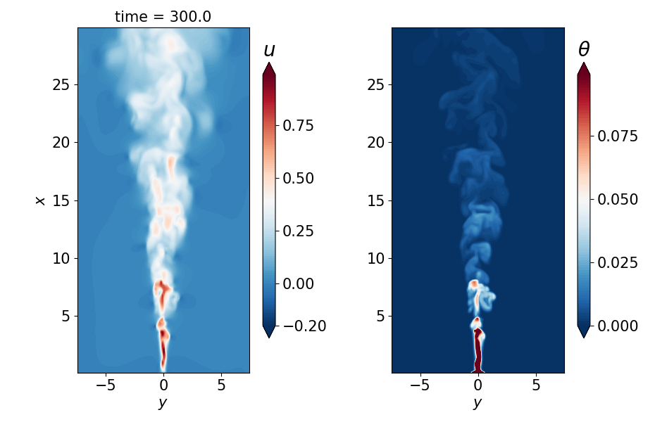
Figure 3: (Left) the vertical velocity and (right) the temperature distributions in a plume at $Re=1000$.

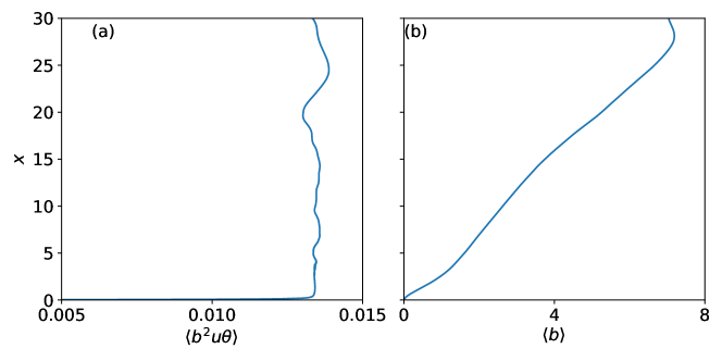
Figure 4: (a): the buoyancy flux $\langle b^{2}u\theta\rangle$, where $\langle\rangle$ denotes an average over the plane and over the time range $200<t<400$, for a plume at Reynolds number $Re=1000$. (b): the plume width, calculated using the mass and momentum fluxes (see eq. 27).

IV Results and Discussion

IV.1 Simulations in one dimension

Equilibrium turbulent plumes, like all free-shear flows, entrain ambient fluid at a rate proportional to a characteristic velocity (Morton et al., 1956). In general, the diffusivities of temperature and vapour could be different, making the problem more complex. Since the diffusivities of temperature and vapour (and liquid) are here assumed to be equal (§II.3), a plume that carries vapour in addition to temperature behaves exactly like a classical plume. This simplification allows a model, following Morton et al. (1956), to be written for such a plume.

Consider a plume of width $b$ and velocity $u$. The mass and momentum fluxes are $M=b^{2}u$ and $P=b^{2}u^{2}$. The vapour and liquid fluxes are $F_{v}=b^{2}ur_{v}$ and $F_{l}=b^{2}ur_{l}$. Assuming a steady state in time, the equations govering the evolution of these quantities with height are

$$\frac{d}{dx}M =2\alpha\left|P\right|^{1/2}$$

$$\frac{d}{dx}P =\frac{M}{P}\left(F+r_{0}\left\{\left(\chi-1\right)\left(F_{v}-r_{v}^{\infty}M\right)-F_{l}\right\}\right)$$

$$\frac{d}{dx}F =-M\left(\Gamma_{u}-\Gamma_{0}\right)+L_{2}C_{d}$$

$$\frac{d}{dx}F_{v} =-C_{d}+2\alpha\left|P\right|^{1/2}r_{v}^{\infty}$$

$$\frac{d}{dx}F_{l} =C_{d}$$ (28)

In order to avoid the singularity at the origin, equations 28 are integrated from initial conditions $M=1,$ $P=1$, $r_{v}=1$, $\theta=1$, $r_{l}=0$. For a given $\epsilon$, the two parameters controlling the dynamics are, as before, $\Gamma_{0}$ and $s_{\infty}$. Note that $\alpha$ is now an externally supplied parameter, and the system of Equations 28 is thus not closed. In fact, finding the dependence of $\alpha$ on the buoyancy distribution in the flow is an open problem with deep implications for climate modelling (Narasimha et al., 2011). We use a value of $\alpha=0.08$ for the results reported here.

The evolution of this idealised plume carrying vapour shows a clear lifting condensation level, defined as the height $x$ where the liquid flux is greater than zero. This is plotted as a function of $\Gamma_{0}$ in Figure 5. Since a constant value of $\alpha$ is reasonable for turbulent plumes, and since the cloud flow behaves like a turbulent plume until condensation sets in at the lifting condensation line (LCL), the results obtained for the height of the LCL may be considered meaningful.

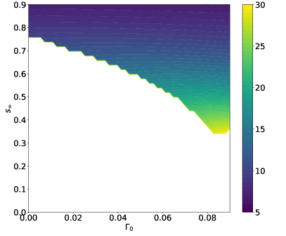
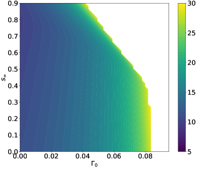
Figure 5: Left: the lifting condensation level predicted from the 1D model in equations 28; and right: the maximum height $h_{max}$ reached; as a function of $s_{\infty}$ and $\Gamma_{0}$.

IV.2 3D simulations

The benefit of formulating the problem in terms of the nondimensional parameters $L_{1},L_{2},\Gamma_{d},\epsilon,Re,\Gamma_{0},s_{\infty}$ (§II.6) is that the same formulation can then be applied to any combination of substances (clouds containing methane vapour and liquid methane in an atmosphere composed mainly of nitrogen, say). Fixing the combination of fluids (air and water vapour/liquid for terrestrial clouds) fixes the parameters $L_{1},L_{2},\Gamma_{d}$, leaving the other four parameters as control parameters. Unless otherwise stated, we fix the Reynolds number $Re=1000$ and the Atwood number $\epsilon=1/30$. Thus, the dynamics of the formation of a cloud (which we will define more precisely in the following) is governed by the combination of only two properties of the ambient: the relative humidity of the ambient $s_{\infty}\left(x\right)$, and the lapse rate of the ambient $\Gamma_{0}$.

First, we note that until the flow carrying vapour reaches the lifting condensation level, its dynamics are similar to that of a plume in a stratified ambient. This can be seen for the case $\Gamma_{0}=0.08$, $s_{\infty}=0.6$ in Figure 6 where no condensation occurs. As we argued in §II.2, the smaller the lapse rate of the ambient, the more stable the stratification is and the harder it is for the plume to overcome it and keep rising. Without the energy input from condensation, therefore, plumes in stably stratified ambients will die out. Whether condensation can help overcome the stable stratification depends on if, before the plume has reached its maximum height, it has either carried up enough vapour with it, or entrained enough vapour from the ambient.

From the above discussion, it may be expected that if the stratification is very stable, a larger background relative humidity will be required for the plume to be sustained. For ambients which are nearly neutrally stratified, even reasonably small levels of background relative humidity will sustain the plume.

Visible clouds are those that contain liquid water droplets. In Figure 7, we show snapshots of the evolution for two cases from table 2. In the first ($s_{\infty}=0.6,\Gamma_{0}=0.09$), the cloud that forms has an LCL at $x\approx 15$, and is fragmented. The second case ($s_{\infty}=0.8,\Gamma_{0}=0.08$) shows a much more vigorous cloud. These cases may be compared with the case presented in Figure 6, where no cloud forms. Figure 8 shows cloud formation in a cases where the atmosphere is almost saturated, with $s_{\infty}=0.9$, and $\Gamma_{0}=0.06$ and $0.065$. These values of $\Gamma_{0}$ are close to the boundary of cloud formation. As a result, the small increase in $\Gamma_{0}$ leads to a dramatic increase in the vigorousness of the convection.

IV.3 Vapour Boundary Conditions

As mentioned in §II.5.1, we study three kinds of boundary conditions for the vapour. These boundary conditions control the amount of vapour introduced into the plume through the hot patch. With increasing vapour in the flow, condensation occurs sooner, thereby lowering the lifting condensation level. In fact, for boundary conditions of the second type (vapour saturated at $\theta=1$), the lifting condensation level could be at $x=0$. These changes, however, do not change the behaviour of the flow qualitatively. A comparison between these boundary conditions is shown in Figure 9.

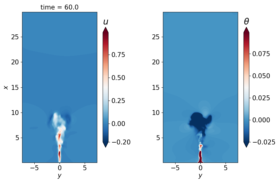
Figure 6: The velocity and temperature for a case where no cloud forms (i.e. the liquid water content $r_{l}=0$). The lapse rate is $\Gamma_{0}=0.08$. The relative humidity $s_{\infty}=60\%$. At the time-instant shown $\left(t=60\right)$, the plume has already hit the maximum height $H_{T}$ and the head of the plume has descended back towards its equilibrium height. Note that $\theta<0$ at the plume-top.

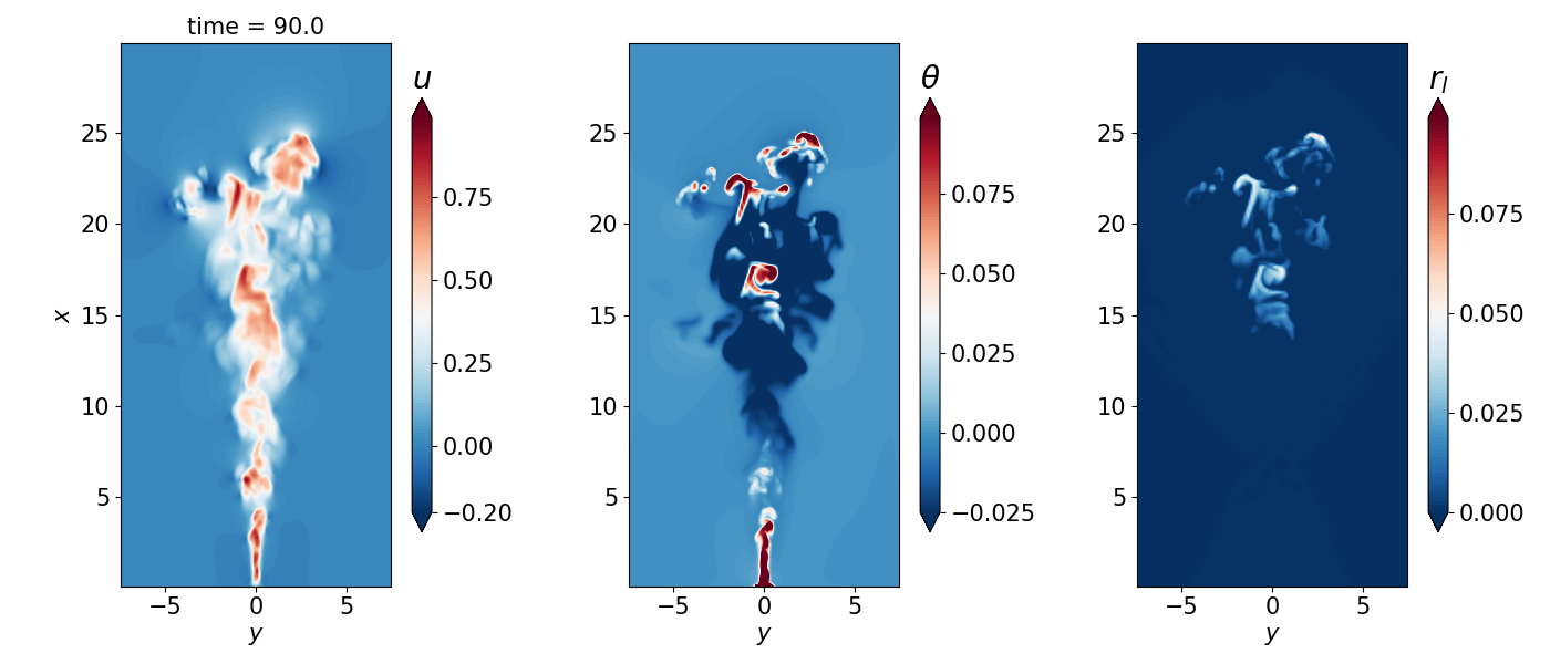
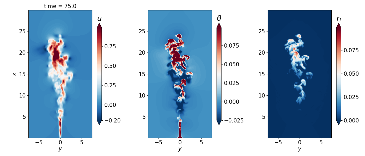
Figure 7: The velocity, temperature excess, and liquid water mixing ratio for (top) $\Gamma_{0}=0.09$, $s_{\infty}=0.6$; and (bottom) $\Gamma_{0}=0.08$, $s_{\infty}=0.8$. The LCL is at a much lower altitude and the ensuing convection is much more vigorous in the latter than in the former. The contours are plotted on the $z=0$ plane.

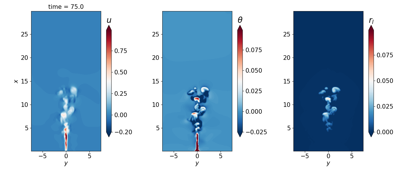
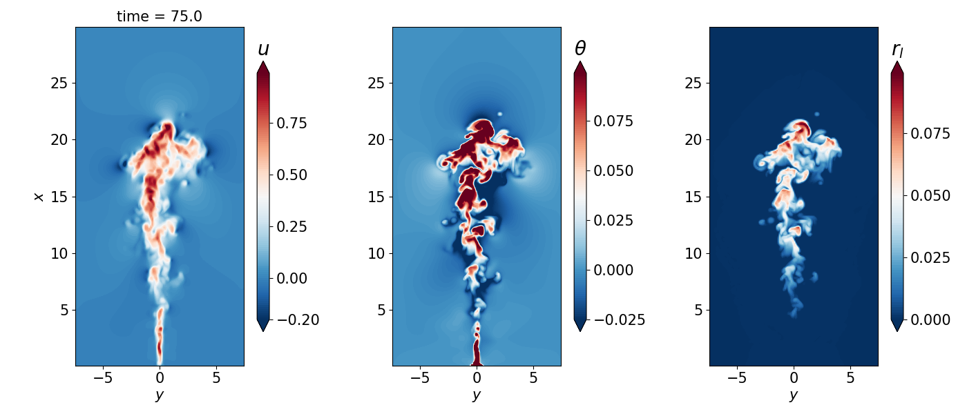
Figure 8: Velocity, temperature and liquid water mixing ratio contours for (top) $\Gamma_{0}=0.06$; and (bottom) $\Gamma_{0}=0.065$, with $s_{\infty}=0.9$ in both cases. A small change in the lapse rate affects the dynamics. The contours are plotted on the $z=0$ plane as before.

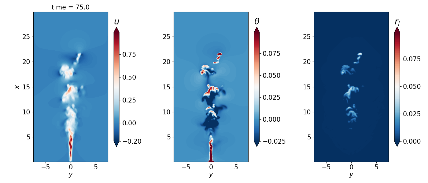
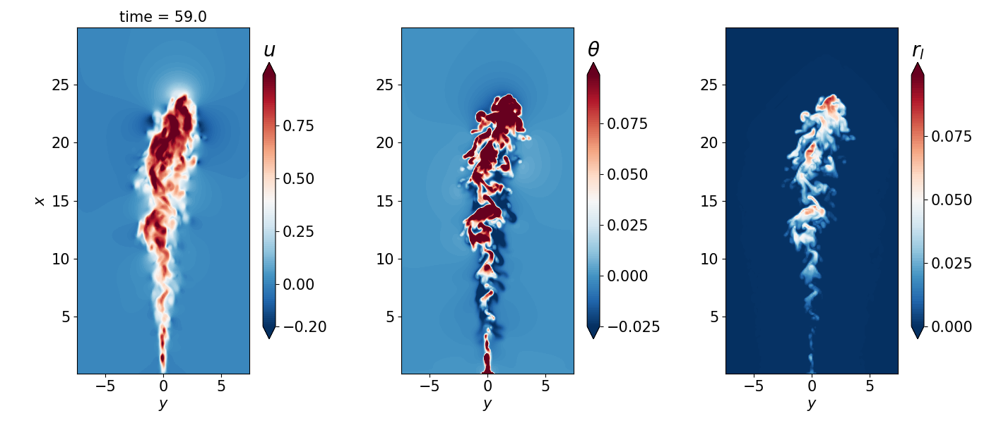
Figure 9: Iso-contours on the $z=0$ plane for $\Gamma_{0}=0.08$ and $s_{\infty}=0.8$, with (top) $r_{v}=s_{\infty}r_{s}\left(\theta=0\right)$; and (bottom) $r_{v}=r_{s}\left(\theta=1\right)$ at the hot patch. The contours are plotted on the $z=0$ plane as before. Note the presence of liquid for all heights in the latter case. Convection becomes increasingly more vigorous as more vapour is introduced into the flow through the hot patch. These may be compared with Fig. 7(b)

IV.4 Cloud–no-cloud boundary

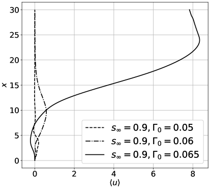
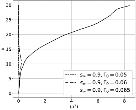
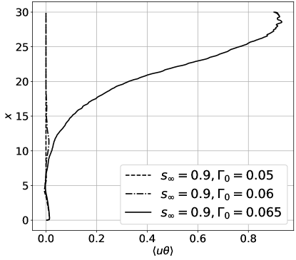
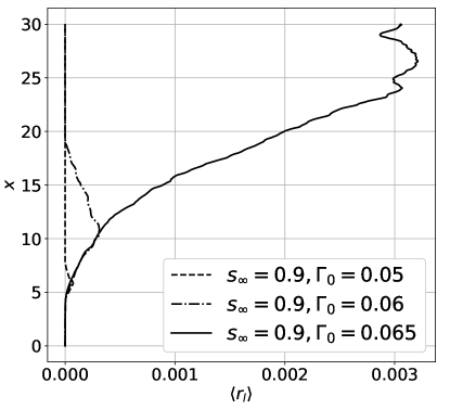
Figure 10: Mass (top-left), momentum (top-right) and buoyancy (bottom-left) fluxes, and the average liquid water content ($r_{l}$) averaged from $t=50$ to $t=100$ as a function of height, showing the influence of increasing lapse rate. The ambient vapour content is fixed at $s_{\infty}=0.9$.

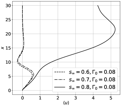
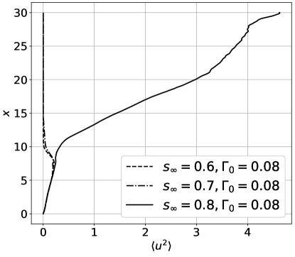
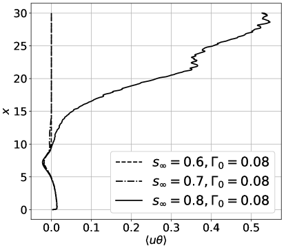
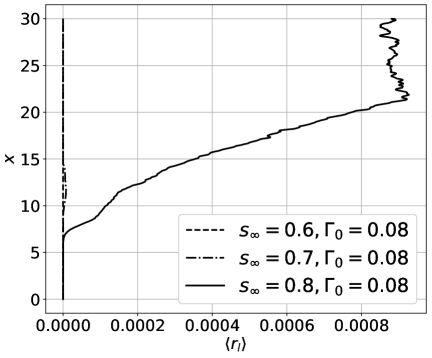
Figure 11: As in Fig. 10, but with a fixed lapse rate and showing the effects of varying $s_{\infty}$.

We now quantify the behaviour of moist plumes as a function of $s_{\infty}$ and $\Gamma_{0}$. For the cases presented in Figs. 6-8, Figures 10 and 11 show the fluxes of mass, momentum and buoancy as a function of height. The cases where clouds form (i.e. where there is a finite amount of liquid water present; also shown in Figs. 10 and 11) show a dramatic increase in these fluxes by up to two orders of magnitude. As expected, these fluxes increase with increasing $s_{\infty}$ and $\Gamma_{0}$. Note that the fluxes with higher ambient vapour content are much larger, even when clouds form in both cases, showing the crucial role played by the energy provided by condensation.

The balance between the background relative humidity and the lapse rate depicted in table 2. In this table, which is drawn in the phase-space of $s_{\infty}$ and $\Gamma_{0}$, the origin (at top left) is an ambient that is completely dry and is very stably stratified. Thus, no cloud will ever form at the origin. The further away from the origin we venture in this space, the easier it is for clouds to form (though we note that traversing along one axis may not be as easy physically as traversing along the other).

This balance is further quantified in Figure 12, where the average liquid water content in the upper half of the domain ($15<x<30$) over $50<t<100$ is plotted as a function of $s_{\infty}$ and $\Gamma_{0}$. This plot and Table 2 may be compared with the predictions from the 1D model in Figs. 5.

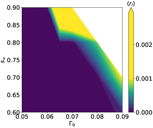
Figure 12: The boundary separating the region in the $s_{\infty}$-$\Gamma_{0}$ space where clouds can or cannot form, drawn using the average liquid flux in the upper half of the domain.

$s_{\infty}$ \$\Gamma_{0}$	$0.05$	$0.06$	$0.065$	$0.07$	$0.08$	$0.09$
$0.6$	x	x	x	x	$\otimes$	$\odot$
$0.7$	x	x	x	x	$\otimes$	$\odot$
$0.8$	x	x	x	$\otimes$	$\odot$	x
$0.9$	$\otimes$	$\odot$	$\odot$	$\odot$	x	x

Table 2: Does a given combination of $s_{\infty}$ and $\Gamma_{0}$ lead to a ‘cloud’? Legend: ‘x’: no simulation; $\otimes$: no cloud; $\odot$: cloud. The presence of a “cloud” is defined as in Fig. 12, by considering the amount of liquid present in the upper half of the domain

IV.5 Plumes versus thermals: models for cumulus convection

As mentioned in §I, cumulus clouds have been alternatively modelled as steady plumes or unsteady thermals. The results here suggest that cumulus clouds are best thought of as steady plumes until the lifting condensation level, and transient diabatic coherent structures after condensation begins. The nature of these coherent structures and the entrainment into them remains a problem of active study.

V Conclusion

We have presented a framework using which the dynamics of cumulus clouds can be studied with direct numerical simulations. This framework relies on the simplification of the Clausius-Clapeyron equation, with consistent approximation of both the dynamics and the thermodynamics, such that the system of equations does not explicitly contain the absolute temperature or the properties of the fluid. We use this framework to show that the formation of cumulus clouds can be described in terms of a small number of parameters, and that the dynamics depends crucially on the relative humidity and the lapse rate of the ambient. In terms of the latter pair of parameters, we show when cumulus clouds may form in a stratified ambient out of the plumes that emanate from a hot patch. We show that there exists a boundary in the $s_{\infty}-\Gamma_{0}$ plane which separates the regions where cumulus clouds can and cannot form. The existence of this boundary, we show, is robust to changes in $Re$ and $\epsilon$ , although where the boundary appears in the $s_{\infty}-\Gamma_{0}$ phase plane does depend on $Re$ and $\epsilon$.

We posit that the long-standing puzzle of anomalous entrainment in cumulus clouds can be resolved through direct numerical simulations of these flows. In this pursuit, our formulation provides a simple framework which includes all the relevant physics while retaining the simplicity that enables the use of high-performance computing. The entrainment in cumulus clouds is the subject of an ongoing study in the group.

References

- Cohn (2017) S. Cohn, WMO Bulletin, Geneva, World Meteorological Organization 66, 2 (2017).
- Stevens and Bony (2013) B. Stevens and S. Bony, Science 340, 1053 (2013).
- Bony et al. (2015) S. Bony, B. Stevens, D. M. Frierson, C. Jakob, M. Kageyama, R. Pincus, T. G. Shepherd, S. C. Sherwood, A. P. Siebesma, A. H. Sobel, et al., Nature Geoscience 8, 261 (2015).
- Bjerknes (1938) J. Bjerknes, Quart. J. Roy. Meteor. Soc. 64, 325 (1938).
- Pruppacher and Klett (2010) H. Pruppacher and J. Klett, Microphysics of Clouds and Precipitation (Springer Netherlands, Dordrecht, 2010) pp. 10–73.
- Narasimha et al. (2011) R. Narasimha, S. S. Diwan, S. Duvvuri, K. Sreenivas, and G. Bhat, Proceedings of the National Academy of Sciences 108, 16164 (2011).
- Grabowski and Wang (2013) W. W. Grabowski and L.-P. Wang, Annual review of fluid mechanics 45, 293 (2013).
- Randall et al. (2003) D. Randall, M. Khairoutdinov, A. Arakawa, and W. Grabowski, Bulletin of the American Meteorological Society 84, 1547 (2003).
- Morton et al. (1956) B. Morton, G. I. Taylor, and J. S. Turner, Proc. R. Soc. Lond. A 234, 1 (1956).
- Turner (1962) J. Turner, Journal of Fluid Mechanics 13, 356 (1962).
- De Rooy et al. (2013) W. C. De Rooy, P. Bechtold, K. Fröhlich, C. Hohenegger, H. Jonker, D. Mironov, A. P. Siebesma, J. Teixeira, and J.-I. Yano, Quarterly Journal of the Royal Meteorological Society 139, 1 (2013).
- Bhat and Narasimha (1996) G. Bhat and R. Narasimha, Journal of Fluid Mechanics 325, 303 (1996).
- Turner (1969) J. Turner, Annual Review of Fluid Mechanics 1, 29 (1969).
- Lecoanet and Jeevanjee (2019) D. Lecoanet and N. Jeevanjee, Journal of the Atmospheric Sciences (2019).
- Pauluis et al. (2010) O. Pauluis, J. Schumacher, et al., Communications in Mathematical Sciences 8, 295 (2010).
- Schumacher and Pauluis (2010) J. Schumacher and O. Pauluis, Journal of Fluid Mechanics 648, 509 (2010).
- Wu et al. (2009) C.-M. Wu, B. Stevens, and A. Arakawa, Journal of the Atmospheric Sciences 66, 1793 (2009).
- Kadanoff (2001) L. P. Kadanoff, Physics today 54, 34 (2001).
- Puthenveettil and Arakeri (2005) B. A. Puthenveettil and J. H. Arakeri, Journal of Fluid Mechanics 542, 217 (2005).
- Morrison et al. (2009) H. Morrison, G. Thompson, and V. Tatarskii, Monthly weather review 137, 991 (2009).
- Kumar et al. (2014) B. Kumar, J. Schumacher, and R. A. Shaw, Journal of the Atmospheric Sciences 71, 2564 (2014).
- Spiegel and Veronis (1960) E. Spiegel and G. Veronis, The Astrophysical Journal 131, 442 (1960).
- Bannon (1996) P. R. Bannon, Journal of the Atmospheric Sciences 53, 3618 (1996).
- Durran (1989) D. R. Durran, Journal of the atmospheric sciences 46, 1453 (1989).
- Hernandez-Duenas et al. (2013) G. Hernandez-Duenas, A. J. Majda, L. M. Smith, and S. N. Stechmann, Journal of Fluid Mechanics 717, 576 (2013).
- Orlanski (1976) I. Orlanski, Journal of computational physics 21, 251 (1976).
- van der Poel et al. (2015) E. P. van der Poel, R. O. Monico, J. Donners, and R. Verzicco, Computers & Fluids 28 (2015), 10.1016/j.compfluid.2015.04.007.
- Prabhakaran (2014) P. Prabhakaran, “Direct numerical simulations of volumetrically heated jets and plumes,” (2014).
- Ravichandran et al. (2020) S. Ravichandran, E. Meiburg, and R. Govindarajan, in review (2020).
- Plourde et al. (2008) F. Plourde, M. V. Pham, S. D. Kim, and S. Balachandar, Journal of Fluid Mechanics 604, 99 (2008).