Cosmic evolution of molecular gas mass density from an empirical relation between $L_{\rm 1.4GHz}$ and $L^{{}^{\prime}}_{\rm CO}$

Abstract

Historically, GHz radio emission has been used extensively to characterize the star-formation activity in galaxies. In this work, we look for empirical relations amongst the radio luminosity, the infrared luminosity, and the CO-based molecular gas mass. We assemble a sample of 278 nearby galaxies with measurements of radio continuum and total infrared emission, and the ¹²CO ($J=1$–0) emission line. We find a correlation between the radio continuum and the CO emission line (with a scatter of 0.36 dex), in a large sample of different kind of galaxies. Making use of this correlation, we explore the evolution of the molecular gas mass function and the cosmological molecular gas mass density in six redshift bins up to $z=1.5$. These results agree with previous semi-analytic predictions and direct measurements: the cosmic molecular gas density increases up to $z=1.5$. In addition, we find a single plane across five orders of magnitude for the explored luminosities, with a scatter of 0.27 dex. These correlations are sufficiently robust to be used for samples where no CO measurements exist.

1 Introduction

Understanding galaxy evolution is a key goal of modern astrophysics. This can be tackled using a wide range of observational and theoretical prescriptions which involve complex physical processes for their interpretation (e.g. Davies et al. 2019). In the cosmological context, a primary focus of this study is the evolution of the cosmic star-formation history (CSFH, e.g. Tinsley & Danly 1980; Madau et al. 1996). Studies based on large galaxy samples reveal that the cosmic star-formation rate (SFR) density peaks at $z\sim 2$–3 then declines steadily by $\sim\,20\times$ through to the present time (Madau & Dickinson, 2014). The physical processes involved are not yet clear, although some of the main predictions are: the growth of the dark-matter halos (e.g. Behroozi et al. 2013), the depletion of molecular gas reservoirs in galaxies (e.g. Kennicutt & Evans 2012; Genzel et al. 2015; Tacconi et al. 2018) and changes in the star-formation efficiency (e.g. Genzel et al. 2010; Daddi et al. 2010).

The molecular gas is the reservoir for the future star-formation (SF) activity, so its census across cosmic time is fundamental to understand CSFH. Historically, the main proxy to trace the molecular gas mass is via the rotational low-$J$ ($J$ = 1–0) transitions of the carbon monoxide (CO) molecule (Bolatto et al., 2013). Recently, spectroscopic surveys undertaken with the Atacama Large Millimeter/submillimeter Array (ALMA, e.g. ASPECS; Walter et al. 2016; Decarli et al. 2016) have revealed that the molecular gas mass density changes by a factor of 3–$10\times$ across $z=0$–2. This result is in concordance with predictions from semi-analytic models (e.g. Popping et al. 2012; Lagos et al. 2018). Nevertheless, when CO-based studies are performed via pencil-beam surveys, they are: (a) naturally affected by cosmic variance (Walter et al., 2016); (b) biased to detect the most intensely star-forming galaxies (e.g. Bothwell et al. 2013) and (c) based on small galaxy samples (e.g. Daddi et al. 2010; Genzel et al. 2010, 2015). These limitations are a consequence of the considerable amount of observing time needed to measure CO lines in galaxies beyond the local Universe.

An alternative but less direct method to measure the gas mass, $M_{\rm gas}$, uses the dust that is concomitant with the molecular gas. Several studies show that optically thin dust emission in the Rayleigh-Jeans regime ($\sim 350$–1000 $\rm\mu m$) is proportional to the dust mass (e.g. Dunne et al. 2011; Clemens et al. 2013; Bianchi 2013), where there is a strong sensitivity on dust temperature (Scoville et al., 2014). Diffuse, cold dust ($T\leq 25$ K) dominates the dust mass in galaxies, while warmer dust ($T\geq 30$ K) usually dominates the dust luminosity (Devereux & Young, 1990; Dunne & Eales, 2001; Draine et al., 2007; Clark et al., 2015). According to Scoville et al. (2014), the molecular gas mass can be obtained from a single measurement of flux density made in a specific band on the Rayleigh-Jeans tail, assuming a typical dust temperature between 20–45 K. Adopting a dust-to-gas mass ratio, these authors then determine the molecular gas mass. Using this method, recent studies (e.g. Scoville et al. 2016; Hughes et al. 2017a) using small samples of massive, nearby, star-forming, infrared-bright galaxies ($L_{\rm IR}>10^{11}$ L_⊙) found empirical relations between the luminosity at 850 $\rm\mu m$ ($L_{850}$) and the total $M_{\rm gas}$. The $L_{850}$—$M_{\rm gas}$ relation is tight (scatter $\sim\,0.3$ dex), which makes it possible to obtain $M_{\rm gas}$ in an efficient, precise manner for large samples of galaxies.

Using a sample $10\times$ larger than that of Scoville et al. (2014), however, Orellana et al. (2017) found that the relation between the submillimetre (submm) emission and the gas mass determined by Scovile’s method shows a significant dispersion ($\sim\,1$ dex), as well as increased scatter towards fainter luminosities. Moreover, Orellana et al. (2017) found that the dust mass is a more accurate tracer of the total gas mass (atomic and molecular) than the molecular gas mass alone, in concordance with recent results obtained by Casasola et al. (2020) based on 436 nearby galaxies from the DustPedia Survey (Davies et al., 2017).

In this paper we construct new scaling relations using other tracers of molecular gas which can provide more precise molecular gas mass estimates with a lower dispersion.

To tackle this problem, we make use of three well-studied relations. First, the radio continuum–infrared (RC–IR) correlation connects the non-thermal radio emission, typically at 1.4 GHz, and the IR radiation coming from dust grains heated by ultraviolet photons from young stellar populations, assuming that supernovae remnants related to massive young stars are responsible for the synchrotron radiation. The RC–IR correlation has been shown to be valid over a wide range of star-forming galaxies (e.g. Bell 2003; Ibar et al. 2008; Ivison et al. 2010; Smith et al. 2014; Liu et al. 2015) with little evolution across the cosmic time (Ivison et al., 2010; Magnelli et al., 2015).

Second, the global Schmidt-Kennicutt (SK) relation connects the formation of stars with the fuel to produce them, i.e. the molecular gas; it can be expressed in terms $L_{\rm IR}$ and $L^{{}^{\prime}}_{\rm CO}$ luminosities, respectively (e.g. Kennicutt & Evans 2012), where $L^{{}^{\prime}}_{\rm CO}$ is the luminosity of the CO molecule, closely related to the molecular gas mass (see e.g. Bolatto et al. 2013).

Third, the other widely used relation exploited here connects the RC and CO emission. The relation between CO luminosity, $L^{{}^{\prime}}_{\rm CO}$, and radio luminosity, $L_{\rm 1.4GHz}$, has been known since early CO observations (e.g. Rickard et al. 1977; Israel, & Rowan-Robinson 1984; Murgia et al. 2002) and probed in the local Universe for different type of galaxies (e.g. disk-like; dwarfs; ultraluminous IR galaxies, ULIRGs) using unresolved observations (global-scale observations; e.g. Adler et al. 1991; Leroy et al. 2005; Liu et al. 2015) as well as in resolved regions down to $\sim 100$ pc (e.g. Murgia et al. 2005; Paladino et al. 2006; Schinnerer et al. 2013).

This article is the first of a series in which we explore the connection between the RC and the IR and the molecular gas mass ($M_{\rm H_{2}}$, traced by the CO luminosity) in spatially resolved galaxies and in galaxies at higher redshifts. We show the use of RC as a relatively precise proxy for the molecular gas mass in the local Universe and beyond. We also present an empirical plane among the RC emission, the IR luminosity and the CO luminosity. We base our work on large samples of galaxies built from wide-area surveys, resulting in more statistically robust work than was previously possible.

Throughout the text, we assume a $\Lambda$-CDM cosmology with $H_{0}=70$  km s^-1 Mpc^-1, $\Omega_{\rm M}=0.3$ and $\Omega_{\Lambda}=0.7$.

2 Sample selection

Our sample is constructed from seven surveys taken from the literature, all of which have measurements of IR, RC and low-$J$ CO lines for galaxies at redshifts, $z<0.3$:

• VALES (Villanueva et al., 2017; Hughes et al., 2017a, b; Cheng et al., 2018; Molina et al., 2019) comprises 91 galaxies at ($0.02<z<0.35$) taken from H-ATLAS (Eales et al., 2010), with 65 galaxies detected spectroscopically in low-$J$ CO ($J=1$–0 or $J=2$–1) using the Atacama Large Millimetre Array (ALMA) or the Atacama Pathfinder EXperiment (APEX). In addition, VALES has rich multi-wavelength coverage from UV to far-IR wavelengths compiled by the Galaxy And Mass Assembly survey (GAMA; Driver et al. 2016), allowing us to measure $L_{\rm IR}$ by spectral energy distribution (SED) fitting. In order to homogenise the CO line measurements to $J=1$–0, we assume a luminosity ratio $L^{\prime}_{\rm CO(2-1)}/L^{\prime}_{\rm CO~{}(1-0)}=0.85$ (as tabulated by Carilli $\&$ Walter, 2013).

• The xCOLD GASS survey (Saintonge et al., 2017) is a recent upgrade of the COLD GASS survey (Saintonge et al., 2011a, b) with the newest sample called COLD GASS-low. In total, xCOLD GASS contains 532 galaxies, both star-forming and passive ellipticals with stellar mass in the range $9.0<\log(M_{*}/{\rm L}_{\odot})<11.5$, in the redshift range, $0.01<z<0.05$, which have been observed with the IRAM 30-m telescope in CO($J=1$–0) and with APEX in CO($J=2$–1). We use only the CO ($J=1$–0) data from this survey. The IR data comes from the Infrared Astronomical Satellite (IRAS; Neugebauer et al. 1984).

• Liu et al. (2015) (hereafter, Liu15) contains 181 local galaxies with IR luminosities between $7.8<\log($$L_{\rm IR}$$/{\rm L}_{\odot})<12.3$, where 115 are normal spiral galaxies and the rest are ULIRGs. This sample contains CO ($J=1$–0) flux measurements from high-resolution CO maps published in the literature (Chung et al., 2009; Young et al., 2008; Kuno et al., 2007; Gao & Solomon, 2004; Helfer et al., 2003; Sofue et al., 2003) and IR data from IRAS.

• The APEX Low-redshift Legacy Survey for MOlecular Gas (ALLSMOG; Cicone et al. 2017) comprises 97 Sloan Digital Sky Survey (SDSS DR7) galaxies at $0.01<z<0.03$, with stellar masses in the range $8.5<\log($$M_{*}$$/{\rm L}_{\odot})<10.0$, classified as star forming according to the BPT diagram and with a gas-phase metallicity 12 + $\log(O/H)\geq 8.5$. In addition, this sample contains measurements of CO($J=1$–0) from the IRAM 30-m telescope and of CO($J=2$–1) from APEX. We use only their CO($J=1$–0) measurements. We derive $L_{\rm IR}$ from the Wide-field Infrared Survey Explorer (WISE) photometry (from the ALLWISE cataloge, Wright et al. 2010) at 12 $\rm\mu m$ following Cluver et al. (2014) .

• The ATLAS^3D survey (Cappellari et al., 2011) contains 260 galaxies — a volume-limited sample ($D<42$ Mpc) of early-type galaxies (ellipticals, E, and lenticulars, S0) brighter than $M_{K}<-21.5$ mag ($\log$$M_{*}$$\geq 9.78$ $\rm M_{\odot}$), where 56 galaxies have both CO($J=1$–0) and ($J=2$–1) measurements from IRAM 30m (Young et al., 2011), from which we only use the values for CO($J=1$–0). For this sample, we derive $L_{\rm IR}$ from WISE photometry (from the ALLWISE cataloge) at 12 $\rm\mu m$ following Cluver et al. (2014).

• Leroy et al. (2005)(hereafter, Leroy05) contains 121 nearby ($v_{\rm LSR}\leq 1,000$ km s^-1) dwarf galaxies with typical dynamical masses $M_{\rm dyn}\leq 10^{10}$ M_⊙, optical diameters $d_{25}<5^{\prime}$, and with atomic hydrogen line widths, $W_{20}\leq 200$ km s^-1, selected from the IRAS Faint Source Catalog (FSC) at 60 and/or 100 $\rm\mu m$. This sample contains 28 galaxies detected (at S/N $\geq 5$) in CO ($J=1$–0) and another 16 galaxies marginally detected (S/N $\sim 3$) from the Arizona Radio Observatory’s 12-m telescope. We derive $L_{\rm IR}$ for this sample from IRAS 60- and 100-$\rm\mu m$ photometry, following Orellana et al. (2017).

• Papadopoulos et al. (2012) (hereafter, Pap12) contains 70 local ($z<0.1$) IR galaxies ($10<\log($$L_{\rm IR}$$/{\rm L}_{\odot})<12$) selected from the IRAS Revised Bright Galaxy Survey (RBGS; Sanders et al. 2003) — a flux-limited sample (flux density at 60 $\rm\mu m$$>5.24$ Jy). Additionally, this sample has coverage of CO($J=1$–0) from the IRAM 30-m telescope.

GAMA	S band	C band	X band	Ku band	$\rm\alpha_{radio}$
ID	[$\mu$Jy]	[$\mu$Jy]	[$\mu$Jy]	[$\mu$Jy]
324931	510$\pm$57	…	…	$138\pm 30$	$-0.81\pm 0.10$
543473	…	$291\pm 22$	$170\pm 11$	$154\pm 20$	$-0.71\pm 0.10$
491545	…	$347\pm 46$	$213\pm 18$	$164\pm 23$	$-0.82\pm 0.13$
15049	…	$93\pm 9$	$12\pm 14$	$63\pm 17$	$-0.58\pm 0.21$
319660	…	$192\pm 28$	$150\pm 16$	$134\pm 25$	$-0.40\pm 0.16$
323772	…	$629\pm 27$	…	…	…
278874	…	$68\pm 11$	…	…	…
346900	…	$174\pm 15$	…	…	…
600656	…	…	…	$45\pm 17$	…
210543	$235\pm 32$	…	…	…	…
378002	$391\pm 47$	…	…	…	…
216973	$740\pm 38$	…	…	…	…

Table 1: New radio continuum data for VALES galaxies (see §2.1) in the S band ($\nu=3$ GHz), C band ($6$ GHz), X band ($10$ GHz) and Ku band ($15$ GHz) bands. The power-law index, $\alpha_{\rm radio}$ ($S\sim\nu^{\alpha_{\rm radio}}$) is obtained from these JVLA measurements and we assume $\alpha_{\rm radio}=-0.7\pm 0.3$ for the galaxies with RC obtained from the literature (see §2.1 for more details).

2.1 Radio data

In this work, we present new radio data for the VALES sample obtained from observations taken with the Karl G. Jansky Very Large Array (JVLA; VLA/13B-376, P.I.: E. Ibar) at 3, 6, 10 and/or 15 GHz, with resolutions between 0$\aas@@fstack{\prime\prime}$6 and 4$\aas@@fstack{\prime\prime}$0 (see Table 1). Additionally we match the VALES sample with the publicly available Faint Images of the Radio Sky at Twenty-Centimeters (FIRST; White et al. 1998) survey at 1.4 GHz,to obtain a larger sample in the radio continuum emission.

We compute the radio spectral index $\alpha$ ($S_{\nu}\propto\nu^{\alpha}$) in five galaxies from the VALES survey with multiple JVLA detections. To measure the flux densities in galaxies with multiple radio band measurements, we use the Common Astronomy Software Applications (CASA, release 5.0.0) (McMullin et al. 2007) task imsmooth to degrade the resolution of the images to a common worst resolution. Then we measure the integrated flux density using the task imfit, which allows us to use the same Gaussian profile in each image.

For non-VALES galaxies, the RC data were gathered as follows. In the case of the Liu15 sample, this catalogue includes its own radio data. For the xCOLD GASS catalogue, we match this sample with the FIRST survey, with a matching radius of 4$\arcsec$. For the rest of the samples (Leroy05, Pap12, ALLSMOG and ATLAS^3D), the measurements at 1.4 GHz are taken from the NRAO VLA Sky Survey (NVSS; Condon et al. 1998) using a matching radius of 20$\arcsec$. To discard possible mismatches, we use the SIMBAD database (Wenger et al., 2000), and we corroborate that several of these galaxies have optical minor axis greater than 60$\arcsec$ and/or that the optical images show no other dominant galaxies within a radius of 60 arcsec.

The continuum radio luminosity was obtained in three different ways: (1) for VALES galaxies with multiple JVLA detections, we $k$-correct the flux density, $S_{\rm 1.4GHz}$, using the measured radio spectral index, including error propagation. These spectral indices and errors were obtained from the best fit based on all the JVLA measurements available; (2) for galaxies with only one JVLA, FIRST or NVSS measurement, we estimate the $k$-corrected $S_{\rm 1.4GHz}$ measurement assuming the typical radio spectral index of $-0.7\pm 0.3$ (Ibar et al. 2009) expected for star-forming galaxies. In this case, the error propagation includes the observed errors and the scatter of the assumed $\alpha$; (3) for galaxies in Liu15 and Leroy05, we use those directly provided by the surveys. Finally, we calculate the radio monochromatic luminosity from $\displaystyle L_{\rm 1.4GHz}=4\pi D_{\rm L}^{2}S_{\rm 1.4GHz}/(1+z),$ where $D_{\rm L}$ is the luminosity distance and $S_{\rm 1.4GHz}$ is the $k$-corrected flux density.

To discard any possible contamination from radio-loud active galactic nuclei (AGN), we matched the entire sample with the 13^th Edition of the Catalog of Quasar and AGNs (Véron-Cetty & Véron, 2010), finding only four galaxies of our final sample to be radio loud, a typical signature of an AGN. We also matched our final sample with the ALLWISE survey , where 90 per cent of our sample have measurements at 3.4, 4.5 and 12 $\rm\mu m$, allowing us to apply the colour-colour criteria defined by Jarrett et al. (2011) to identify AGNs. We found five galaxies to be AGNs. In summary, $\sim 3$ per cent of our final sample have possible AGN-related contamination of their RC emission. AGN-contaminated galaxies will often show an excess of 1.4 GHz emission with respect to the sample selected as star-forming galaxies. Fig. 1 shows no statistically significance from AGN contamination, confirming that making corrections for any excess in the RC emission is unnecessary.

2.2 Final sample

Final Sample	Original	Reference
(# of galaxies)	Sample
30	VALES	Villanueva et al. (2017)
12	VALES (APEX)	Cheng et al. (2018)
75	xCOLD GASS	Saintonge et al. (2017)
67	Liu15	Liu et al. (2015)
36	Pap12	Papadopoulos et al. (2012)
28	ATLAS3D	Cappellari et al. (2011)
17	ALLSMOG	Cicone et al. (2017)
13	Leroy05	Leroy et al. (2005)
RC	Original	Reference
(# of galaxies)	Sample
12	VALES	This work
189	NVSS	Condon et al. (1998)
77	FIRST	White et al. (1998)
IR	Original	Reference
(# of galaxies)	Sample
42	H-ATLAS	Eales et al. (2010)
142	IRAS	Neugebauer et al. (1984)
36	IRAS RBGS	Sanders et al. (2003)
13	IRAS FSC	Moshir & et al. (1990)
45	ALLWISE	Wright et al. (2010)
CO($J=1$–0)	Original	Reference
(# of galaxies)	Sample
30	VALES	Villanueva et al. (2017)
75	xCOLD GASS	Saintonge et al. (2017)
36	Pap12	Papadopoulos et al. (2012)
28	ATLAS3D	Cappellari et al. (2011)
17	ALLSMOG	Cicone et al. (2017)
13	Leroy05	Leroy et al. (2005)
67	Literature	Chung et al. (2009)
		Young et al. (2008)
		Kuno et al. (2007)
		Gao & Solomon (2004)
		Helfer et al. (2003)
		Sofue et al. (2003)
12∗	VALES (APEX)	Cheng et al. (2018)

Table 2: Summary of the surveys and references used to produce our final sample, indicating the number of galaxies having RC, IR and CO data in each case.
^∗CO data for these galaxies have been converted from CO($J=2$–1)

.

Our final catalogue contains 278 galaxies, where 42 are part of the VALES sample, 67 from Liu15, 75 from xCOLD GASS, 36 from Pap12, 28 from ATLAS^3D, 17 from ALLSMOG and 13 from Leroy05 (see Table 2 for more details). This sample is characterised by: (1) CO line measurements with S/N $>5$ for luminosities ranging from $\displaystyle 5.78<\log\left(L^{\prime}_{\rm CO}/{\rm[K\ km\,s^{-1}\,pc^{2}]}\right)<10.35$, (2) radio detections at S/N $>5$ resulting in a radio luminosity range of $18.64<\log\left(L_{\rm 1.4GHz}/{\rm[W/Hz]}\right)<23.78$, (3) redshifts, $z\leq 0.271$, with a median value, $z=0.017$ and (4) total $L_{\rm IR}$ ranging from $7.3<\log\left(L_{\rm IR}/{\rm[L_{\odot}]}\right)<12.14$. While the total number of galaxies in these seven samples is $>1,000$, we discarded the majority of them either because they are not consistent with our S/N criteria or because they do not have CO, RC or total IR measurements. Additionally, to avoid aperture inconsistencies amongst measurements from different studies, we remove from the sample all galaxies with CO apertures smaller than the Petrosian aperture in the $r$ band or the optical angular diameter obtained from NED

3 Results

Relation	Slope	Intercept		Pearson
	m	b	$\sigma$	coefficient
$L_{\rm 1.4GHz}$–$L_{\rm IR}$	$0.96\pm 0.02$	$11.98\pm 0.23$	0.33	0.934
$L^{{}^{\prime}}_{\rm CO}$–$L_{\rm IR}$	$0.94\pm 0.02$	$-0.98\pm 0.21$	0.29	0.946
$L^{{}^{\prime}}_{\rm CO}$–$L_{\rm 1.4GHz}$	$1.04\pm 0.02$	$-14.09\pm 0.21$	0.36	0.928

Table 3: Best-fit parameters for each relation shown in Fig.1 ($\log(y)=m\times\log(x)+b$). In all these relations, the null hypothesis is rejected. The $\sigma$ value is measured from the scatter, shown in the respective relations.

3.1 The evolution of the RC–CO relation

In order to build a RC–CO relation, we first use a RC–IR correlation that is dependent on redshift, together with the IR–CO correlation. For the RC–IR correlation, we use the result obtained by Magnelli et al. (2015):

$$\log\left(\frac{L_{\rm IR}}{\rm[W]}\right)=\frac{(2.35\pm 0.08)}{\left(1+z\right)^{\left(0.12\pm 0.04\right)}}+\log\left(\frac{L_{\rm 1.4GHz}}{\rm[W\,Hz^{-1}]}\right)+12.85,$$ (1)

where $L_{\rm IR}$ is the total integrated IR luminosity (rest-frame 8–1,000 $\rm\mu m$), $z$ is the redshift, and $L_{\rm 1.4GHz}$ is the radio continuum luminosity at 1.4 GHz. This relation was obtained from a sample of $\sim 340,000$ galaxies at $z<2$.

For the IR–CO correlation, we use the results obtained from Villanueva et al. (2017) based on the VALES sample. They showed that the global $L^{{}^{\prime}}_{\rm CO}$-$L_{\rm IR}$ relation can be represented, thus:

$$\log\left(\frac{L_{\rm IR}}{\rm[W]}\right)=(0.95\pm 0.04)\times\log\left(\frac{L^{\prime}_{\rm CO}}{\rm[K\,km\,s^{-1}\,pc^{2}]}\right)+(28.6\pm 0.4),$$ (2)

where the $L^{{}^{\prime}}_{\rm CO}$ is the CO ($J=1$–0) luminosity.

Finally, combining the RC–IR and the IR–CO relations (equations 1 and 2), we obtain an expression for the RC–CO relation as a function of redshift:

$$\log \left(\frac{L^{\prime}_{\rm CO}}{\rm[K\,km\,s^{-1}\,pc^{2}]}\right)=(2.47\pm 0.13)\times(1+z)^{(-0.12\pm 0.04)}$$ (3)

$$~{}~{}~{}~{}~{}+(1.05\pm 0.04)\times\log\left(\frac{L_{\rm 1.4GHz}}{\rm[W\,Hz^{-1}]}\right)-(16.5\pm 0.8).$$

Errors were propagated assuming a Gaussian probability distribution. For simplicity, we define eq. LABEL:eq:MV as $\xi\left(L_{\rm 1.4GHz},z\right)$.

Fig. 1 shows the RC–IR (top panel), IR–CO (middle panel) and RC–CO (bottom panel) relations, respectively. Although the samples are different, our fitted solutions and scatter ($<0.33$ dex, see Table 3) for the RC–IR and the IR–CO plots are in agreement with the respective results by eq. 1 and eq. 2 (black line). Additionally, the newly constructed RC–CO relation, based on equations 1 and 2, closely matches the best fit of our sampled data.

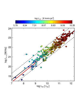
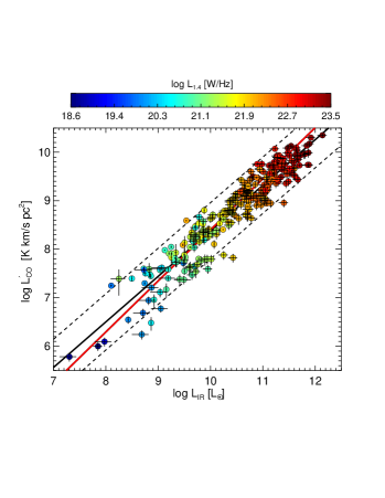
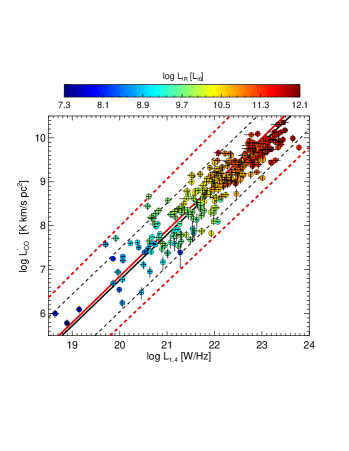
Figure 1: Panels are the $L_{\rm 1.4GHz}$–$L_{\rm IR}$ relation with $L^{{}^{\prime}}_{\rm CO}$ in colour (top), the $L^{{}^{\prime}}_{\rm CO}$–$L_{\rm IR}$ relation with $L_{\rm 1.4GHz}$ in colour (middle), and the $L^{{}^{\prime}}_{\rm CO}$–$L_{\rm 1.4GHz}$ relation with $L_{\rm IR}$ in colour (bottom). Black lines shows the best linear fit (continuous) and 1-$\sigma$ dispersion (dashed). Red lines are the results from equations 1, 2 and LABEL:eq:MV, for top, middle and bottom panels, respectively, assuming the median redshift of the sample, $z=0.017$, for equations 1 and LABEL:eq:MV). Red segmented lines in the bottom panel shows the error of the relation $L^{{}^{\prime}}_{\rm CO}$–$L_{\rm 1.4GHz}$, obtained by propagating the errors in in eq. LABEL:eq:MV.

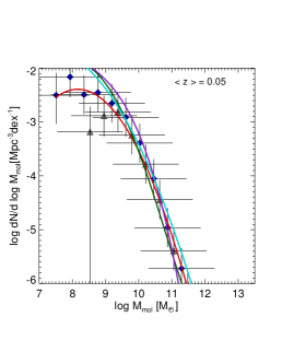
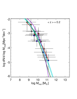
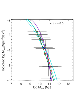
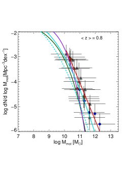
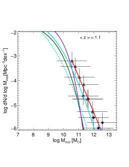
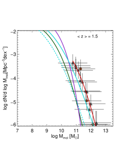
Figure 2: Evolution of the MGMF. The upper-left panel shows the local ($<z>=0.05$) MGMF for star-forming galaxies, from RCLF measured by MS07 (blue diamonds) and Pr16 (gray triangles). The rest of the panels show the MGMF for star-forming galaxies at $<z>=0.2,0.5,0.8,1.1$ and $1.5$ from RCLF measured by N017 (red diamonds), Sm09 (gray triangles) and Pa11 (brown circles). Red lines are the best-fit mass function for all available points, purple and dark green lines are the MGMF from the Popping et al. (2012) and Lagos et al. (2018) models, respectively. Additionally, the cyan solid line is the MGMF from the RCLF model from Smolčić et al. (2009) in combination with eq. LABEL:eq:MV and constant $\alpha_{\rm CO}=3.6~{}{\rm[M_{\odot}/(K\,km\,s^{-1}\,pc^{2})]}$ ; similarly, cyan dashed lines in all plots correspond to the same MGMF but for a constant redshift of $z=0.05$. The errors in the molecular mass are the quadrature addition of the errors from measurements in each work and the scatter obtained in our relations.

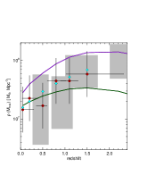
Figure 3: Cosmic molecular mass density ($\rho_{(M_{\rm mol})}$) for the redshift range 0–1.5. Red points are the integrated values for the entire mass range available for the MGMFs from Fig. 2. Cyan points, purple and dark green lines are the integrated MGMF from the Smolčić et al. (2009), Popping et al. (2012) and Lagos et al. (2018) models, in the mass range $9<log(M_{mol}$/$\rm M_{\odot}$)$<11$, respectively. Gray rectangles is the $\rho_{(M_{\rm mol})}$ obtained by Decarli et al. (2016).

3.2 The RC–CO correlation used to estimate the molecular gas mass function

Sample	N∘	Redshift	Alias	References
	bins	range
NVSS/6dFGS	1	0.003–0.3	MS07	Mauch et al. 2007
FIRST/SDSS	1	0.005–0.3	Pr16	Pracy et al. 2016
VLA/COSMOS	4	0.1–1.3	Sm09	Smolčić et al. 2009
VLA/CDF-S	4	0.03–2.3	Pa11	Padovani et al. 2011
VLA/COSMOS	11	0.1–5.7	No17	Novak et al. 2017

Table 4: Radio continuum luminosity function surveys.

One of our most relevant results is that we have found a RC–CO correlation for a large sample as a function of redshift, from eq. LABEL:eq:MV. The sample includes galaxies with different Hubble types at distances greater than 250 Mpc over a wide range of RC and CO line measurements. Because the $L_{\rm 1.4GHz}$ is related to $L^{{}^{\prime}}_{\rm CO}$ which is in turn related to the molecular gas mass, $M_{\rm mol}$, via a linear relation, it is possible to estimate the molecular gas mass function (MGMF, $\phi(M_{\rm mol})$) using RC luminosity function (RCLF, $\phi(L_{\rm RC})$) measured at different redshifts in samples of galaxies which exclude the galaxies contaminated by radio-loud AGN. Then, if we replace $\log L_{\rm 1.4GHz}$ by $\phi(L_{\rm RC})$ in eq. LABEL:eq:MV, we obtain the CO luminosity relation as a function of the redshift. Consequently, by applying eq. LABEL:eq:MV to well-measured RCLFs from the literature (see table 4), we can obtain the CO luminosity functions across the redshift range $0.003<z<5.7$, subdivided into several redshift bins. Although part of the data taken from literature to construct our final sample reach almost $z\sim 6$, our results are constrained up to $z=1.5$ based mainly on the redshift constraints included in eq. 1 and eq. 2.

To predict radio luminosity functions independently of the availability of radio continuum data, we can use the evolution of the RCLF using the model proposed by Smolčić et al. (2009). In this scenario, the local RCLF is based on the model proposed by Sadler et al. (2002), using a combination of a power-law and a Gaussian distribution of the form:

$$\phi_{z=0}\left(L_{\rm RC}\right)=\phi^{*}\left(\frac{L_{\rm RC}}{L_{*}}\right)^{1-\alpha}\exp\left[\frac{-1}{2\sigma^{2}}\left(\log\left[1+\frac{L_{\rm RC}}{L_{*}}\right]\right)^{2}\right],$$ (4)

with a power-law index, $\alpha=0.84$, a luminosity function at the faint end of $\phi^{*}=22.9\times 10^{-3}\,{\rm[Mpc^{-3}]}$, a standard deviation of the Gaussian distribution, $\sigma=0.94$, and a characteristic luminosity limit between the power-law and the Gaussian distribution, $L_{*}=1.95\times 10^{19}\,{\rm[W\,Hz^{-1}]}$ (for more details, see Sadler et al. 2002; Smolčić et al. 2009). Consequently, the evolution of the luminosity function is:

$$\phi\left(L_{\rm RC},z\right)=\phi_{z=0}\left(\frac{L_{\rm RC}}{(1+z)^{\alpha_{\rm L}}}\right),$$ (5)

where $\phi_{z=0}$ is the local luminosity function and a $\alpha_{\rm L}$ is the characteristic luminosity function parameter, with value $\alpha_{\rm L}=2.1\pm 0.2$ (Sadler et al., 2002).

$L^{{}^{\prime}}_{\rm CO}$ is calculated using eq. LABEL:eq:MV and is used to obtain the CO luminosity functions, transforming equations 4 and 5 as follows:

$$\phi_{z=0}\left(L^{\prime}_{\rm CO}\right) =\xi\left(\phi_{z=0}\left(L_{\rm 1.4GHz}\right)\right)$$ (6)

$$\phi\left(L^{\prime}_{\rm CO},z\right) =\xi\left(\phi\left(L_{\rm 1.4GHz},z\right)\right)$$

Finally, to obtain the MGMF, we use the conversion factor between $L^{{}^{\prime}}_{\rm CO}$ and the molecular gas mass, $M_{\rm mol}=\alpha_{\rm CO}$ $L^{{}^{\prime}}_{\rm CO}$, with constant $L^{{}^{\prime}}_{\rm CO}$–$\alpha_{\rm CO}$, where $\alpha_{\rm CO}$ is the molecular mass conversion factor and has a value 3.6 M_⊙/(K km s^-1 pc²). Although this value for $\alpha_{\rm CO}$ does not take into account the helium contribution (the fraction of He is 36 per cent), we adopt it considering that the reference sample to compare our resulting luminosity functions, Decarli et al. (2016), uses this value.

We compare our results with those obtained from the semi-analytic MGMF models developed by Popping et al. (2012) and Lagos et al. (2018). Fig. 2 shows the MGMFs (red and cyan lines) estimated for six redshift bins centred at $<z>=0.05,0.2,0.5,0.8,1.1$ and $1.5$, covering the redshift range from 0.003–2.3. Each sample used is identified by different symbols and colours (see the caption to Fig. 2). The errors result from the addition in quadrature of the error from the original RCLF and the scatter in the $L^{{}^{\prime}}_{\rm CO}$–$L_{\rm 1.4GHz}$ correlation. The purple (Popping et al., 2012) and dark green (Lagos et al., 2018) lines corresponds to semi-analytic models.

Although we could potentially construct a RCLF up to $z=5.7$, our results for the MGMF show a considerable over-estimate in comparison with the semi-analytic models for RCLF at redshifts $z>1.5$. This problem can be caused by: a) the $L^{{}^{\prime}}_{\rm CO}$–$L_{\rm 1.4GHz}$ correlation function evolving with redshift in a different way than that considered in this work; b) it may be incorrect to adopt a constant $\alpha_{\rm CO}$ given that starburst galaxies are more abundant at higher redshifts; c) the RCLM at higher redshifts only characterises the galaxies richest in molecular gas, as a consequence of the detection limit in the radio images; d) semi-analytic models may under-estimate the molecular gas mass at high redshift. Additionally, with the assumption of a constant $\alpha_{\rm CO}$, we ignore any possible variation of the conversion factor as a function of galaxy properties, where the most important property is the dependence on gas-phase metallicity (e.g. Wilson 1995; Arimoto et al. 1996; Barone et al. 2000; Israel 2000; Boselli et al. 2002; Magrini et al. 2011; Schruba et al. 2012; Hunt et al. 2015; Amorín et al. 2016).

3.3 Cosmic molecular gas mass content

Based on the results obtained from our MGMF analysis, we can predict the molecular gas mass density and its evolution with cosmic time. Molecular gas mass density is defined as:

$$\rho_{(M_{\rm mol})}=\int^{\log M_{2}}_{\log M_{1}}\frac{dN}{d\log M~{}dV}~{}M~{}d\log M.$$ (7)

Fig. 3 shows the resulting $\rho_{(M_{\rm mol})}$ in the redshift range $0<z<1.5$, where the red points are derived using the entire mass range available from the respective RCLF. This means that this derived $\rho_{(M_{\rm mol})}$ has different integration mass limits in different redshift bins. For this reason, we make use of the RCLF from Smolčić et al. (2009) to obtain a continuous MGMF where we can extrapolate a fixed integration mass limit to compare our results with the predictions from semi-analytic models. After fixing the integration mass limit in the range $9<\log(M_{\rm mol}/{\rm M}_{\odot})<11$ (the range deduced from the MGMFs obtained by Decarli et al. 2016, but not specified in that work) we can then determine the $\rho_{(M_{\rm mol})}$ based on our continuous MGMF (cyan diamonds). Our results fall inside the errors of the direct measurements obtained by Decarli et al. (2016) (gray rectangles), while the semi-analytic models show higher and lower values for the models from (Popping et al. (2012) (purple line) and Lagos et al. (2018) (green line), respectively.

The main source of uncertainty in $\rho_{(M_{\rm mol})}$ comes from the uncertainty in the measured RC luminosity functions.

3.4 The empirical CO–RC–IR plane

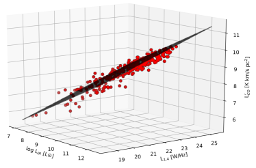
Figure 4: The CO–RC–IR plane. Red circles are the galaxies from the final sample and the black plane is the best fit shown in eq. 8. See more views in Appendix A

Although the physical parameters used for the star-formation relations in this paper — the IR, CO and RC emission — are all tracers of newly formed stars, to our knowledge there is no previous use in the literature of parameter space combining all of them in a single relation. Fig. 1 shows that these three parameters vary in a correlated way. Based on that, we conclude that each panel corresponds to the projection of a CO–RC–IR plane. We present the 3D view of these three relations in Fig. 4 forming a plane for which we obtained a numerical expression using the MPFIT algorithm (Markwardt, 2009):

$$\log \rm\left(\frac{L^{\prime}_{\rm CO}}{\rm[K\,km\,s^{-1}\,pc^{2}]}\right)=(0.61\pm 0.05)\times\log\left(\frac{L_{\rm IR}}{\rm[L_{\odot}]}\right)$$ (8)

$$~{}~{}~{}~{}~{}~{}~{}~{}+(0.36\pm 0.05)\times\log\left(\frac{L_{\rm 1.4GHz}}{\rm[W\,Hz^{-1}]}\right)-(5.4\pm 0.7)~{}.$$

For different views of the plane based on eq. 8, see Appendix A.

4 Discussion

4.1 Cosmic evolution of molecular gas

The intimate connection between the RC, CO and IR emission during the process of forming stars is well established for samples of galaxies. However, understanding the mechanism that links these three parameters remains a challenge for star-formation models, considering the different physical origins for the different emission.

Several tracers of star-formation activity exist. Direct methods include tracing the UV light from young stellar populations. However, UV attenuation by dust in galaxies requires additional corrections. For example, it has been proposed that the emission at 24 $\rm\mu m$ can be used to correct the dust attenuation in far-UV (FUV) and H$\alpha$ data, resulting in more realistic estimates of the SFR in galaxies (Kennicutt et al., 2007; Calzetti et al., 2007). These combined calibrations of SFR are used extensively for nearby galaxies (e.g. Rahman et al. 2011; Ford et al. 2013; Momose et al. 2013; Casasola et al. 2017)

To avoid correcting for extinction, IR emission is widely used as a star-formation tracer. Two energy sources contribute to the IR spectral energy distribution (SED): a warm dust component, where grains absorb UV photons from young, massive ($>8$ $\rm M_{\odot}$) stars (e.g. Devereux, & Young 1991; Condon 1992), and a cold dust component — a consequence of the absorption of optical photons from the interstellar radiation field (e.g. Xu, & Helou 1996). The IR emission is a powerful star-formation tracer, better than other more direct indicators that are affected by extinction (e.g. H_α emission systematically under-estimates, by an order of magnitude, the formation of stars in galaxies with SFR $\geq 20$ $\rm M_{\odot}$ yr^-1 Cram et al. 1998).

The RC emission results from the combined contribution of thermal emission — free-free radiation from H ii regions related to the number of massive, short-lived stars — and non-thermal emission — synchrotron radiation produced by relativistic electrons interacting with the magnetic field of the galaxy (Condon, 1992). These two components dominate the RC at different frequencies, where the transition between the thermal and non-thermal component happens at $\nu\approx 30$ GHz (emission at higher frequencies is mainly thermal and at lower frequencies is mainly synchrotron). Condon (1992) suggests that thermal radiation contributes less than 10 per cent of the total RC radiation at $\sim 1$ GHz and that the total radio luminosity at 1.4 GHz is directly proportional to the supernovae (SN) rate. Synchrotron radio emission from star-forming galaxies is produced by the interaction of energetic electrons — accelerated by the massive stars when they have reached the supernovae stage — and the ambient magnetic field (Israel, & Rowan-Robinson, 1984; Voelk, 1989). Radio emission is unaffected by dust absorption, making RC emission an ideal tool to calibrate other tracers of star formation.

Lastly, CO emission is the consequence of the interaction between CO molecules and the molecular hydrogen (H₂) in regions where stars are formed — giant molecular clouds (GMC). CO emission is correlated with the virial mass of GMCs observed in the Milky Way and in nearby spiral galaxies (Young, & Scoville, 1991).

Historically, the IR–RC–CO parameters have been studied using three empirical relations, each one having different properties: first, the RC–IR correlation (e.g. Yun et al. 2001; Ivison et al. 2010; Thomson et al. 2014; Magnelli et al. 2015; Dumas et al. 2011; Tabatabaei et al. 2013a, b), valid up to $z\sim 2$ and at a resolution of $\geq 500$ pc. Second, the Schmidt-Kennicutt (SK) IR–CO law (Kennicutt, 1998; Kennicutt & Evans, 2012), valid for high-SFR, bright galaxies as well as low-surface-brightness galaxies with low SFR. The form of the SK law is still debated because the observations of disk and starburst galaxies have shown that this relation can be fitted either by a single or a bi-modal solution for the redshifts range 0.05–2.5 (e.g. Genzel et al. 2010; Daddi et al. 2010; Ivison et al. 2011; Kennicutt & Evans 2012; Tacconi et al. 2013; Santini et al. 2014; Freundlich et al. 2019). The slope of the SK law, which defines the depletion time of the gas in a galaxy ($\tau_{\rm dep}\equiv M_{\rm gas}/{\rm SFR}$), is central to our understanding of the mechanisms that govern star formation. According to models, a linear slope implies that star-formation activity is not driven only by the self gravity of the galaxy (Semenov et al., 2017, 2019). Several studies dedicated to the spatially-resolved KS relation on sub-kpc scales found a wide range in the value of the slope (indicated by the power law index, $N\sim 0.6$–3; $\Sigma_{\rm SFR}\propto\Sigma_{M(\rm H_{2})}^{N}$) of the KS relation (Bigiel et al., 2008; Kennicutt & Evans, 2012; Rahman et al., 2011; Viaene et al., 2014; Casasola et al., 2015). The spread in the value of $N$ may be intrinsic, suggesting that different SF relations exist; alternatively, it may be due to the assumptions adopted in each study. Daddi et al. (2010) suggest that $L_{\rm IR}$ (tracing SFR) and $L^{{}^{\prime}}_{\rm CO}$ (tracing molecular gas mass) show no evolution in normal star-forming galaxies up to $z=1.5$. However, Tacconi et al. (2018) suggest that $\tau_{\rm dep}\propto(1+z)^{-0.62}$, implying that $\tau_{\rm dep}$ decreases by a factor of $\approx 2\times$, up to the redshift limit explored in our study, $z=1.5$. Third, the RC–CO correlation (e.g. Adler et al. 1991; Murgia et al. 2002, 2005; Leroy et al. 2005; Paladino et al. 2006; Schinnerer et al. 2013; Liu et al. 2015), is valid for different galaxy types and also down to scales of few hundred parsecs in some selected local galaxies.

In this work we derive eq. LABEL:eq:MV by combining RC–IR and IR–CO relations from the literature to obtain the molecular gas mass density of the Universe, after deriving the integrated MGMF from measurements of the RCLF corrected by $\alpha_{\rm CO}=3.6~{}{\rm[M_{\odot}/(K\,km\,s^{-1}\,pc^{2})]}$. We find that the resulting molecular gas mass density increases by a factor of $4.4\times$ across $z=0.05$–1.5. As mentioned above, we expect that the evolution of the depletion time has little impact on our final gas mass densities.

4.2 Using the CO–RC–IR plane to predict CO emission in galaxies

Several authors have proposed models to explain the physical connection between the radio, infrared and CO luminosities. One of the earliest models proposes that the RC–IR correlation is physically linked to the formation of young massive stellar populations (e.g. Helou et al. 1985; Condon 1992) since GMCs collapse to form stars of large masses, responsible for an intense radiation field in star-forming galaxies. A large fraction of the UV photons from the forming stars heat the dust grains, re-processing the UV radiation into IR emission. Considering that the main mechanism that drives this model (Adler et al. 1991; Murgia et al. 2002) is the formation of new stars, it is expected that $L^{{}^{\prime}}_{\rm CO}$ — a classical tracer of the gas reservoir for future star formation — is correlated with IR and RC emission. As a first approach, this model offers a simple mechanism to explain how these three parameters can be related by considering that the origin of the IR emission and the non-thermal synchrotron corresponds to newly formed stars in molecular clouds. However, this model is unable to explain several problems, e.g. why the RC–IR correlation is maintained at scales of kpc and the RC–CO relation holds at scales of $\sim 100$ pc. In addition, Schinnerer et al. (2013) argue that this model requires too many intermediate physical processes to observationally correlate both the RC and the IR emission, where each of these processes has to contribute to a larger scatter than that obtained from observations. Alternative models, e.g. the calorimeter model (Voelk 1989; Lisenfeld et al. 1996), the magnetic field-gas density coupling (Helou, & Bicay 1993; Niklas, & Beck 1997), and the proton calorimeter model (Suchkov et al., 1993; Lacki et al., 2010) also struggle to explain the physical mechanisms involved in these relations.

Our work provides an empirical solution that combines CO–RC–IR into a plane, which can be exploited to update star-formation models. We find that our proposed plane — where the CO, RC, and IR luminosities are fitted simultaneously — results in smaller scatter for each of the relations than when they are fitted independently in pairs. For example, the comparison between the estimated $L^{{}^{\prime}}_{\rm CO}$ obtained using eq. 8 and the actual measured $L^{{}^{\prime}}_{\rm CO}$ shows a scatter of 0.27 dex (a factor $1.86\times$). The scatter between our sample and the IR–CO and RC–CO relations are 0.29 and 0.36 dex, respectively (see Table 3). As a consequence, the CO–RC–IR plane constitutes a powerful tool to predict, in a very efficient way, the CO emission in large samples of galaxies lacking molecular mass measurements. Although the CO–RC–IR plane is fitted using a wide range of galaxy types (local LIRGs, massive star-forming galaxies, elliptical galaxies with star formation, dwarf galaxies), the scatter for the predicted CO emission from the plane is lower than the scatter from independent use of the IR–CO or RC–CO relations.

Using a sample of $\sim 80$ metal-rich and -poor dwarf galaxies, Filho et al. (2019) studied the star-forming relations RC–IR, RC–CO and IR–CO finding that they cannot be extended down to low radio luminosity dwarfs. A breakdown for the dwarfs appears towards brighter radio luminosities in both relations with respect to the solution for bright galaxies from Price & Duric 1992; Liu & Gao 2010; Kennicutt et al. 2011; Murgia et al. 2005. According to Filho et al. (2019), the breakdown in the RC–CO and IR–CO relations reflects a depletion of CO in dwarf galaxies, which have a hard ionising radiation field, low dust shielding and slower chemical reaction rates, making this molecule an inefficient tracer of molecular gas. Cosmic rays from starburst episodes also play a role in destroying the CO molecules. We cannot directly compare Filho et al. (2019)’s results with our work because the range of luminosities for their sample of dwarfs is about an order of magnitude fainter than ours.

Considering that each parameter used in the construction of the plane involves observed emission coming directly or indirectly from the formation of stars, the simplest scenario to explain the existence of this three-fold relation lies with models where star formation is the main driver. Assuming that star formation is the main driver behind the observed consistency of RC, IR, CO emission, then implementing it to predict CO emission on a different sample requires the selection of star-forming galaxies only, where no contribution of AGN is present.

5 Summary

In summary, we have used 278 nearby ($z<0.27$) galaxies with measurements of global CO lines ($J=1$–0 or $J=2$–1), total IR luminosity and radio continuum flux density at 1.4 GHz to study the scaling relations between the CO, RC, and IR luminosities and to determine the cosmic evolution of the molecular gas content of the Universe. Assuming that star formation is the main mechanism that drives the existence of the SK (IR–CO) and RC–IR relations, we derive the RC–CO relation as a function of redshift. This relation allows us to estimate the molecular gas mass function (MGMF) using the radio continuum luminosity function (RCLF) from the literature, obtaining consistent results as compared with the MGMF from semi-analytic models across $0.05<z<1.5$. Finally, from the integration of the different MGMFs, we estimate the cosmic evolution of the molecular gas mass density ($\rho(M_{\rm mol})$) in star-forming galaxies, in six redshift bins, showing an increment of $4.4\times$ across this redshift range.

In addition, we found that these three luminosities ($L^{{}^{\prime}}_{\rm CO}$, $L_{\rm 1.4GHz}$ and $L_{\rm IR}$) form a plane, presumably as a consequence of the common physical mechanisms behind these three observable quantities in the context of star formation in galaxies. The plane is valid across more than five orders of magnitude for each of the luminosities, across the redshift range 0.05–0.27, and it can be used to predict CO emission from the IR and radio continuum measurements of galaxies, with a scatter of 0.27 dex. The agreement of our estimates with semi-analytical models, as well as with the results from the ALMA large programme, ASPECS, is a clear indication of the power of the method presented here as a tool to predict molecular gas mass at different cosmic epochs. Future large radio surveys, such as those conducted by the Square Kilometer Array, will be able to exploit these results.

Appendix A The best-fit plane

This appendix includes different views of the plane $L^{{}^{\prime}}_{\rm CO}$–$L_{\rm 1.4GHz}$ — $L_{\rm IR}$. The black lines in Fig. 1 show the best-fit plane, shown in eq. 8; the red circles are the galaxies in our final sample.

Using this plane, it is clear that the dispersion shown is tiny compared with the large range of IR, RC and CO used in our work.

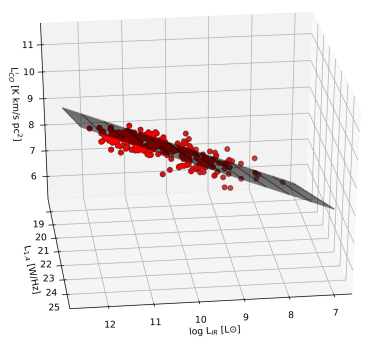
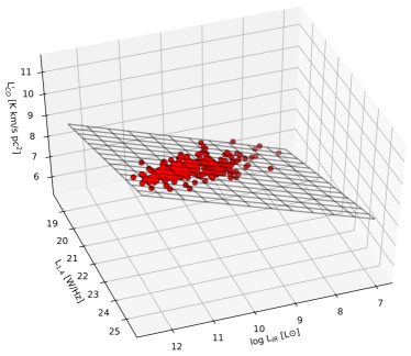
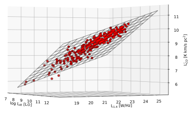
Figure 5: Different views of the plane for $L^{{}^{\prime}}_{\rm CO}$—$L_{\rm 1.4GHz}$—$L_{\rm IR}$. The red circles are the galaxies from the final sample and the black plane is the best fit shown in eq. 8.

References

- Adler et al. (1991) Adler D. S., Allen R. J., Lo K. Y., 1991, ApJ, 382, 475
- Amorín et al. (2016) Amorín, R., Muñoz-Tuñón, C., Aguerri, J. A. L., et al. 2016, A&A, 588, A23
- Arimoto et al. (1996) Arimoto, N., Sofue, Y., & Tsujimoto, T. 1996, PASJ, 48, 275
- Barone et al. (2000) Barone, L. T., Heithausen, A., Hüttemeister, S., et al. 2000, MNRAS, 317, 649
- Behroozi et al. (2013) Behroozi, P. S., Wechsler, R. H., et al. 2013, ApJ, 770, 57
- Bell (2003) Bell, E. F. 2003, ApJ, 586, 794
- Bianchi (2013) Bianchi, S. 2013, A&A, 552, A89
- Bigiel et al. (2008) Bigiel, F., Leroy, A., Walter, F., et al. 2008, AJ, 136, 2846
- Bolatto et al. (2013) Bolatto, A. D., Wolfire, M., et al. 2013, ARA&A, 51, 207
- Boselli et al. (2002) Boselli, A., Lequeux, J., & Gavazzi, G. 2002, Ap&SS, 281, 127
- Bothwell et al. (2013) Bothwell, M. S., Smail, I., et al. 2013, MNRAS, 429, 3047
- Cappellari et al. (2011) Cappellari, M., Emsellem, E., et al. 2011, MNRAS, 413, 813
- Carilli Walter (2013) Carilli C. L., Walter F., 2013, ARAA, 51, 105
- Casasola et al. (2020) Casasola, V., Bianchi, S., De Vis, P., et al. 2020, A&A, 633, A100
- Casasola et al. (2017) Casasola, V., Cassarà, L. P., Bianchi, S., et al. 2017, A&A, 605, A18
- Casasola et al. (2015) Casasola, V., Hunt, L., Combes, F., et al. 2015, A&A, 577, A135
- Calzetti et al. (2007) Calzetti, D., Kennicutt, R. C., Engelbracht, C. W., et al. 2007, ApJ, 666, 870
- Cheng et al. (2018) Cheng, C., Ibar, E., et al. 2018, MNRAS, 475, 248
- Chung et al. (2009) Chung, A., van Gorkom, J. H., Kenney, J. D. P., et al. 2009, AJ, 138, 1741
- Cicone et al. (2017) Cicone, C., Bothwell, M., Wagg, J., et al. 2017, A&A, 604, A53
- Clark et al. (2015) Clark, C. J. R., Dunne, L., Gomez, H. L., et al. 2015, MNRAS, 452, 397
- Clemens et al. (2013) Clemens, M. S., Negrello, M., De Zotti, G., et al. 2013, MNRAS, 433, 695
- Cluver et al. (2014) Cluver, M. E., Jarrett, T. H., et al. 2014, ApJ, 782, 90
- Condon et al. (1998) Condon, J. J., Cotton, W. D., et al. 1998, AJ, 115, 1693
- Condon (1992) Condon, J. J. 1992, ARA&A, 30, 575
- Cram et al. (1998) Cram, L., Hopkins, A., Mobasher, B., et al. 1998, ApJ, 507, 155
- Daddi et al. (2010) Daddi, E., Elbaz, D., et al. 2010, ApJ, 714, L118
- Davies et al. (2017) Davies, J. I., Baes, M., Bianchi, S., et al. 2017, PASP, 129, 044102
- Davies et al. (2019) Davies, L. J. M., Lagos, C. del P., Katsianis, A., et al. 2019, MNRAS, 483, 1881
- Decarli et al. (2016) Decarli, R., Walter, F., et al. 2016, ApJ, 833, 69
- Devereux & Young (1990) Devereux, N. A., & Young, J. S. 1990, ApJ, 359, 42
- Devereux, & Young (1991) Devereux, N. A., & Young, J. S. 1991, ApJ, 371, 515
- Draine et al. (2007) Draine, B. T., Dale, D. A., Bendo, G., et al. 2007, ApJ, 663, 866
- Driver et al. (2016) Driver, S. P., Wright, A. H., et al. 2016, MNRAS,455, 3911
- Dumas et al. (2011) Dumas, G., Schinnerer, E., Tabatabaei, F. S., et al. 2011, AJ, 141, 41
- Dunne & Eales (2001) Dunne, L., & Eales, S. A. 2001, MNRAS, 327, 697
- Dunne et al. (2011) Dunne, L., Gomez, H. L., da Cunha, E., et al. 2011, MNRAS, 417, 1510
- Eales et al. (2010) Eales, S., Dunne, L., Clements, D., et al. 2010, PASP, 122, 499
- Filho et al. (2019) Filho, M. E., Tabatabaei, F. S., Sánchez Almeida, J., et al. 2019, MNRAS, 484, 543
- Ford et al. (2013) Ford, G. P., Gear, W. K., Smith, M. W. L., et al. 2013, ApJ, 769, 55
- Freundlich et al. (2019) Freundlich, J., Combes, F., Tacconi, L. J., et al. 2019, A&A, 622, A105
- Gao & Solomon (2004) Gao, Y., & Solomon, P. M. 2004, ApJ, 606, 271
- Genzel et al. (2010) Genzel, R., Tacconi, L. J., et al. 2010, MNRAS, 407, 2091
- Genzel et al. (2015) Genzel, R., Tacconi, L. J., Lutz, D., et al. 2015, ApJ, 800, 20
- Helfer et al. (2003) Helfer, T. T., Thornley, M. D., Regan, M. W., et al. 2003, ApJS, 145, 259
- Helou, & Bicay (1993) Helou, G., & Bicay, M. D. 1993, ApJ, 415, 93
- Helou et al. (1985) Helou, G., Soifer, B. T., & Rowan-Robinson, M. 1985, ApJ, 298, L7
- Hughes et al. (2017a) Hughes, T. M., Ibar, E., et al. 2017, A&A, 602, A49
- Hughes et al. (2017b) Hughes, T. M., Ibar, E., Villanueva, V., et al. 2017, MNRAS, 468, L103
- Hunt et al. (2015) Hunt, L. K., García-Burillo, S., Casasola, V., et al. 2015, A&A, 583, A114
- Ibar et al. (2008) Ibar, E., Cirasuolo, M., Ivison, R., et al. 2008, MNRAS, 386, 953
- Ibar et al. (2009) Ibar, E., Ivison, R. J., et al. 2009, MNRAS, 397, 281
- Israel, & Rowan-Robinson (1984) Israel, F., & Rowan-Robinson, M. 1984, ApJ, 283, 81
- Israel (2000) Israel, F. 2000, Molecular Hydrogen in Space, 293
- Ivison et al. (2010) Ivison, R. J., Magnelli, B., Ibar, E., et al. 2010, A&A, 518, L31
- Ivison et al. (2011) Ivison, R. J., Papadopoulos, P. P., Smail, I., et al. 2011, MNRAS, 412, 1913
- Jarrett et al. (2011) Jarrett, T. H., Cohen, M., Masci, F., et al. 2011, ApJ, 735, 112
- Kennicutt & Evans (2012) Kennicutt, R. C., & Evans, N. J. 2012, ARA&A, 50, 531
- Kennicutt et al. (2011) Kennicutt, R. C., Calzetti, D., Aniano, G., et al. 2011, PASP, 123, 1347
- Kennicutt (1998) Kennicutt R. C., 1998, ApJ, 498, 541
- Kennicutt et al. (2007) Kennicutt, R. C., Calzetti, D., Walter, F., et al. 2007, ApJ, 671, 333
- Kuno et al. (2007) Kuno, N., Sato, N., Nakanishi, H., et al. 2007, PASJ, 59, 117
- Lacki et al. (2010) Lacki, B. C., Thompson, T. A., & Quataert, E. 2010, ApJ, 717, 1
- Lagos et al. (2018) Lagos, C. d. P., Tobar, R. J., et al. 2018, MNRAS, 481, 3573
- Leroy et al. (2005) Leroy A., Bolatto A. D., Simon J. D., Blitz L., 2005, ApJ, 625, 763
- Lisenfeld et al. (1996) Lisenfeld, U., Voelk, H. J., & Xu, C. 1996, A&A, 306, 677
- Liu et al. (2015) Liu, L., Gao, Y., & Greve, T. R. 2015, ApJ, 805, 31
- Liu & Gao (2010) Liu, F., & Gao, Y. 2010, ApJ, 713, 524
- Madau & Dickinson (2014) Madau, P., & Dickinson, M. 2014, ARA&A, 52, 415
- Madau et al. (1996) Madau, P., Ferguson, H. C., Dickinson, M. E., et al. 1996, MNRAS, 283, 1388
- Magnelli et al. (2015) Magnelli, B., Ivison, R. J., Lutz, D., et al. 2015, A&A, 573, A45
- Magrini et al. (2011) Magrini, L., Bianchi, S., Corbelli, E., et al. 2011, A&A, 535, A13
- Mauch et al. (2007) Mauch, T., & Sadler, E. M. 2007, MNRAS, 375, 931
- Markwardt (2009) Markwardt, C. B. 2009, Astronomical Data Analysis Software and Systems XVIII, 411, 251
- McMullin et al. (2007) McMullin, J. P., Waters, B., et al. 2007, Astronomical Data Analysis Software and Systems XVI, 376, 127
- Molina et al. (2019) Molina, J., Ibar, E., Villanueva, V., et al. 2019, MNRAS, 482, 1499
- Momose et al. (2013) Momose, R., Koda, J., Kennicutt, R. C., et al. 2013, ApJ, 772, L13
- Moshir & et al. (1990) Moshir, M., & et al. 1990, IRAS Faint Source Catalogue (ver. 2.0; Pasadena: IPAC)
- Murgia et al. (2005) Murgia M., Helfer T. T., Ekers R., Blitz L., Moscadelli L., Wong T., Paladino R., 2005, A&A, 437, 389
- Murgia et al. (2002) Murgia M., Crapsi A., Moscadelli L., Gregorini L., 2002, A&A, 385, 412
- Neugebauer et al. (1984) Neugebauer, G., Habing, H. J., et al. 1984, ApJ, 278, L1
- Niklas, & Beck (1997) Niklas, S., & Beck, R. 1997, A&A, 320, 54
- Novak et al. (2017) Novak, M., Smolčić, V., Delhaize, J., et al. 2017, A&A, 602, A5
- Orellana et al. (2017) Orellana, G., Nagar, N. M., et al. 2017, A&A, 602, A68
- Padovani et al. (2011) Padovani, P., Miller, N., et al. 2011, ApJ, 740, 20
- Paladino et al. (2006) Paladino, R., Murgia, M., Helfer, T. T., et al. 2006, A&A, 456, 847