Casimir forces on deformed fermionic chains

Abstract

We characterize the Casimir forces for the Dirac vacuum on free-fermionic chains with smoothly varying hopping amplitudes, which correspond to (1+1)D curved spacetimes with a static metric in the continuum limit. The first-order energy potential for an obstacle on that lattice corresponds to the Newtonian potential associated to the metric, while the finite-size corrections are described by a curved extension of the conformal field theory predictions, including a suitable boundary term. We show that, for weak deformations of the Minkowski metric, Casimir forces measured by a local observer at the boundary are metric-independent. We provide numerical evidence for our results on a variety of (1+1)D deformations: Minkowski, Rindler, anti-de Sitter (the so-called rainbow system) and sinusoidal metrics.

I Introduction

The quantum vacuum on a static spacetime is nothing but the ground state (GS) of a certain Hamiltonian. Therefore, it is subject to quantum fluctuations which help minimize its energy. Yet, these fluctuations are clamped near the boundaries, giving rise to the celebrated Casimir effect Casimir.48 , see Klimchitskaya.06 for experimental confirmations. Its relevance extends away from the quantum realm, with applications to thermal fluctuations in fluids Kardar.99 . Its initial description required two infinite parallel plates, giving rise to an attractive force between them. In fact, this attraction was rigorously proved for identical plates by Kenneth and Klich Kenneth.06 , yet the force can become repulsive or even cancel out when the boundary conditions do not match Asorey.13 . The special features of fermionic 1D systems have also been considered Sundberg.04 ; Zhabinskaya.08 .

For fields subject to conformal invariance, the Casimir force is associated to the conformal anomaly, measured by the central charge in 2D conformal field theory (CFT), $c$ Cardy.84 ; Cardy.86 ; DiFrancesco ; Mussardo . The expression for the energy contains a non-universal contribution proportional to the system size, plus finite-size corrections of order $O(1/N)$ which are fixed by conformal invariance. Moreover, conformal invariance is strong enough to yield an analytical expression for the Casimir forces in presence of arbitrarily shaped boundaries Bimonte.13 .

The peculiarities of Casimir forces in curved spacetimes have been considered by several authors DeWitt.75 . The problem is already difficult for static spacetimes and weak gravitational fields Sorge.05 ; Sorge.19 ; Nouri.10 ; Nazari.12 . The Casimir force takes the same form on weak static gravitational fields at first-order, when coordinate differences are substituted by actual distances, although with non-trivial second-order corrections. Interestingly, the Casimir effect has been put forward as a possible explanation of the cosmological constant, making use of Lifshitz theory Leonhardt.19 ; Leonhardt.20 .

Even if our technological abilities do not allow us to access direct measurements of the Casimir effect in curved spacetimes, we are aware of possible strategies to develop quantum simulators using current technologies, such as ultracold atoms in optical lattices Lewenstein.12 . Concretely, it has been shown that the Dirac vacuum on certain static spacetimes can be characterized in such a quantum simulator Boada.11 , and an application has been devised to measure the Unruh radiation, including its non-trivial dimensional dependence Laguna_unruh.17 ; Takagi.86 ; Louko.18 . The key insight is the use of curved optical lattices, in which fermionic atoms are distributed on a flat optical lattice with inhomogeneous hopping amplitudes, thus simulating a position-dependence index of refraction or, in other terms, an optical metric.

Dirac vacua in such curved optical lattices present quite novel properties. When the background metric is negatively curved, i.e.: (1+1)D anti-de Sitter (AdS), the entanglement entropy (EE) may violate maximally the area law Eisert.10 , forming the so-called rainbow state Vitagliano.10 ; Ramirez.14 ; Ramirez.15 . Interestingly, the EE of blocks within the GS of a (1+1)D system with conformal invariance is fixed by CFT Holzhey.94 ; Vidal.03 ; Calabrese.04 ; Calabrese.09 . Such conformal arguments can be extended to a statically deformed (1+1)D system, and the EE of the rainbow system was successfully predicted Laguna.17 , along with other interesting magnitudes, such as the entanglement spectrum, entanglement contour and entanglement Hamiltonian Tonni.18 ; MacCormack.18 .

The aim of this article is to extend the aforementioned (1+1)D CFT predictions on curved backgrounds to characterize the Casimir force for the fermionic vacuum on curved optical lattices. This article is organized as follows. In Sec. II we describe our physical system and summarize the CFT techniques employed to evaluate the EE on curved backgrounds, providing some examples. Sec. III characterizes the Casimir forces on curved optical lattices, using the same example backgrounds, emphasizing the role of universality in the finite-size corrections. The article closes with a series of conclusions and proposals for further work.

II Fermions on curved optical lattices

Let us consider an open fermionic chain with (even) $N$ sites, whose Hilbert space is spanned by creation operators $c^{\dagger}_{m}$, $m\in\{1,\cdots,N\}$ following standard anticommutation relations. We can define an inhomogeneous hopping Hamiltonian,

$$H(\textbf{J})_{N}=-\sum_{m=1}^{N-1}J_{m}c^{\dagger}_{m}c_{m+1}+\text{h.c.},$$ (1)

where $\textbf{J}=\{J_{m}\}_{m=1}^{N-1}$ are the hopping amplitudes, $J_{m}\in{\mathbb{R}}^{+}$ referring to the link between sites $m$ and $m+1$, see Fig. 1 (a). In order to obtain some physical intuition, let us remember that the set of $\{J_{m}\}$ constitutes a position-dependent Fermi velocity, i.e.: a signal takes a time of order $J_{m}^{-1}$ to travel between sites $m$ and $m+1$. If the $\{J_{m}\}$ are smooth enough, we can assume $J_{m}=J(x_{m})$ for a certain smooth function $J(x)$, with $x_{m}=m\Delta x$. Unless otherwise specified, we will use $\Delta x=1$.

It can be proved that Eq. (1) is a discretized version of the Hamiltonian for a Dirac fermion on a curved (1+1)D spacetime with a static metric of the form Boada.11 ; Ramirez.15 ; Laguna.17

$$ds^{2}=-J^{2}(x)dt^{2}+dx^{2},$$ (2)

i.e. a spacetime metric with a position dependent speed of light or, equivalently, a modulated index of refraction. Defining $\tilde{x}(x)$ such that

$$d\tilde{x}=\frac{dx}{J(x)},$$ (3)

we have

$$ds^{2}=J^{2}(x)(-dt^{2}+d\tilde{x}^{2}),$$ (4)

which is conformally equivalent to the Minkowski metric. This deformation is illustrated in Fig. 1 (b): sites get closer when the $J_{m}$ associated to their link is large, giving rise to an homogeneous effective hopping amplitude.

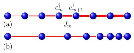
Figure 1: (a) Illustration of an inhomogeneous chain with $N=8$ sites. (b) Corresponding positions after the deformed coordinates $\tilde{x}$.

Conformal equivalence between metrics (4) and the Minkowski metric suggests that conformal field theory (CFT) techniques might describe the universal properties of low-energy eigenstates of Hamiltonian (1). Indeed, we will show that this is the case, once those universal properties have been ascertained.

Some interesting metrics fall into this category. If $J(x)=J_{0}$ is a constant, we recover Minkowski spacetime on a finite spatial interval. The Rindler metric, which is the spacetime structure perceived by an observer moving with constant acceleration $a$ in a Minkowski metric, is described by

$$J(x)=J_{0}+ax.$$ (5)

Notice that it presents an horizon at $x_{h}=-J_{0}/a$, where the local speed of light vanishes. Information can not cross this point, thus separating spacetime into two Rindler wedges Wald . We will consider some other choices for the hopping amplitudes, such as the sine metric,

$$J(x)=J_{0}+A\sin\left(kx\right),$$ (6)

or a rainbow metric given by

$$J(x)=J_{0}\exp\left(-h\left|x-\frac{N}{2}\right|\right),$$ (7)

for $h\geq 0$, with $h=0$ corresponding to the Minkowski case. This metric has constant negative curvature except at the center, $x=N/2$, thus resembling an anti-de Sitter (adS) space, and has been considered recently because its vacuum presents volumetric entanglement Vitagliano.10 ; Ramirez.14 ; Ramirez.15 ; Laguna.17 ; Tonni.18 ; MacCormack.18 . Unless otherwise stated, we will always assume $J_{0}=1$.

II.1 Free fermions on the lattice

The exact diagonalization of Hamiltonian (1) is a straightforward procedure which only involves the solution of the associated single-body problem. Let us define the hopping matrix, $T_{ij}=T_{ji}=-J_{i}\delta_{i,j+1}$, such that

$$H(\textbf{J})_{N}=-\sum_{i,j}T_{ij}c^{\dagger}_{i}c_{j},$$ (8)

then we can diagonlize the hopping matrix, $T_{ij}=\sum_{k}U_{i,k}\epsilon_{k}\bar{U}_{j,k}$, where $\epsilon_{k}$ are the single-body energies and the columns of $U_{i,k}$ represent the single-body modes. The GS of Hamiltonian (1) can be written as $\left|\Psi\right>=\prod_{k=1}^{N/2}b^{\dagger}_{k}\left|0\right>$, where $\left|0\right>$ is the Fock vacuum and $b^{\dagger}_{k}=\sum_{i}U_{i,k}c^{\dagger}_{i}$.

The system presents particle-hole symmetry, $\epsilon_{k}=-\epsilon_{N+1-k}$, with $U_{i,k}=(-1)^{i}U_{i,N+1-k}$. At half-filling the local density is always homogeneous, $\left<c^{\dagger}_{n}c_{n}\right>=1/2$ for all $n$, independently of the metric. For the Minkowski metric,

$$\left<c^{\dagger}_{n}c_{n+1}\right>=\sum_{k=1}^{N/2}\bar{U}_{n,k}U_{n+1,k}\approx{c_{0}\over 2}\equiv{1\over\pi},$$ (9)

plus a correction term presenting parity oscillations, related to the fact that the Fermi momentum is $k_{F}=\pi/2$.

II.2 CFT and entanglement for curved lattice fermions

Let us provide a cursory summary of the application of CFT techniques to the characterization of the entanglement structure of the fermionic vacuum on curved optical lattices.

The von Neumann entanglement entropy (EE) of a block $A$ of a pure state $\left|\Psi\right>$ is defined as

$$S_{A}=-\text{\rm Tr}\left[\rho\log\rho_{A}\right],$$ (10)

where $\rho_{A}=\text{\rm Tr}_{\bar{A}}\left|\Psi\right>\left<\Psi\right|$ is the reduced density matrix for block $A$. In the case of Gaussian states, which follow Wick’s theorem, this magnitude can be determined from the two-point correlation function with low computational effort Peschel.03 . Following Calabrese.04 ; Calabrese.09 , the EE of a lateral block $A=\{1,\cdots,\ell\}$ of the GS of a conformal system with central charge $c$ on a chain with $N$ sites can be written as

$$S(\ell)={c\over 6}\log\left({N\over\pi\Delta x}\sin\left({\pi\ell\over N}\right)\right)+S_{\text{non-univ}}.$$ (11)

where $c=1$ for free fermions, $\Delta x$ is the UV cutoff and $S_{\text{non-univ}}$ is a non-universal contribution containing a constant term and parity oscillations which has been explicitly computed for the free-fermionic case Jin.04 ; Fagotti.11 .

Expression (11) has been successfully extended to evaluate entanglement entropies on the GS of Hamiltonian (1) Laguna.17 ; Tonni.18 . When Dirac fermions are inserted in a smooth static optical metric of the type (2), the EE deforms appropriately, i.e. the block lengths must be transformed via Eq. (3),

$$\ell\to\tilde{\ell}=\tilde{x}(\ell\Delta x)=\int_{x_{0}}^{\ell\Delta x}{dx\over J(x)}\approx\sum_{p=1}^{\ell-1}{\Delta x\over J_{p}},$$ (12)

while $\tilde{N}=\tilde{x}(N\Delta x)$. We must also take into account the transformation of the UV cutoff,

$$\Delta x\;\to\;\Delta\tilde{x}(\ell)=\frac{\Delta x}{J(\ell)}.$$ (13)

Thus, we obtain

$$S(\ell)={c\over 6}\log\left({\tilde{N}\over\pi\Delta\tilde{x}}\sin\left({\pi\tilde{\ell}\over\tilde{N}}\right)\right)+S_{\text{non-univ}}.$$ (14)

Concretely, in Laguna.17 ; Tonni.18 the EE for lateral blocks within the GS of the rainbow Hamiltonian (1) using (7) was obtained using

$$\Delta\tilde{x} =e^{-h|N/2-\ell|}\Delta x,$$ (15)

$$h\tilde{N} =2(e^{hN/2}-1)\Delta x,$$ (16)

$$h\tilde{\ell} =\begin{cases}\left(e^{hN/2}-e^{h(N/2-\ell)}\right)\Delta x,&\text{if }\ell\leq N/2,\\ \left(e^{hN/2}+e^{h(\ell-N/2)}\right)\Delta x,&\text{if }\ell\geq N/2.\\ \end{cases}$$ (17)

In the limit $h\ell\gg 1$, the EE of a block of size $\ell\leq N/2$ becomes

$$S(\ell)\approx{ch\over 6}\ell+S_{\text{non-univ}},$$ (18)

i.e. it yields a volume law for entanglement Tonni.18 , violating maximally the so-called area law of entanglement Eisert.10 . We can also apply Eq. (14) to the case of the Rindler metric, where we find

$$S(\ell)={1\over 6}\log\left({\ell\log N\over\pi\Delta x}\sin\left({\pi\log(N/\ell)\over\log N}\right)\right)+S_{\text{non-univ}}.$$ (19)

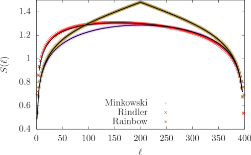
Figure 2: Entanglement entropy of the GS of free fermionic systems on a optical chain with $N=400$ for three different metrics: Minkowski, rainbow (Eq. (7) with $h=0.01$) and Rindler (Eq. (5) with $a=2$), using the procedures of Peschel.03 The continuous lines are the CFT prediction, given by Eq. (14), with a non-universal constant term added.

The validity of these expressions can be checked in Fig. 2, where we have plotted the entropy $S_{A}$ as a function of the block size $l$ for three systems using $N=400$: the Minkowski case, Eq. (11), the rainbow case with $h=0.01$, Eq. (14) with (17), and the Rindler case with $a=2$, via Eq. (19). Indeed, the non-universal terms are present, which also carry parity oscillations, but they are a small correction to the entanglement entropy as predicted by the CFT.

The accuracy of the CFT prediction allows us to conjecture that free Dirac fermions on curved optical lattices can be characterized by a suitable deformation of a conformal field theory, expecting that the non-universal terms will be small enough. We will put this conjecture to the test in the next section.

III Casimir forces on curved optical lattices

Let us characterize the Casimir forces on curved optical lattices in successive approximations. First of all, we will show that the GS energy of Hamiltonian (1) is proportional to the sum of the hoppings in first-order perturbation theory. This will lead us to show that the force felt by a classical obstacle immerse in that state will be similar to the Newtonian gravitational force in the corresponding metric. Then, we will reach the main result of this work: the finite-size corrections to the Casimir energy are universal, and the corresponding expressions are a deformed variant of the general CFT form.

III.1 Potential energy and correlator rigidity

Let us consider a free fermionic chain of $N$ sites on a deformed metric, following Eq. (1). The exact vacuum energy can be written as

$$E_{N}=-2\sum_{p=1}^{N-1}J_{p}\;\textrm{Re}\langle c^{\dagger}_{p}c_{p+1}\rangle.$$ (20)

We can estimate this expression via perturbation theory, if we assume that $J_{p}=J_{0}+\delta J_{p}$ and make use of Eq. (9). The result at first-order is

$$E_{0}\approx-c_{0}S_{N},\qquad\text{where }S_{N}\equiv\sum_{p=1}^{N-1}J_{p}.$$ (21)

The validity of this approximation can be checked in the top panel of Fig. 3, for four different metrics: Minkowski, Rindler, Sine and Rainbow. The accuracy of our conjecture suggests that the local correlators in the deformed vacuum are still homogeneous. In fact, we will make the further claim that the local correlators are rigid, i.e. $\langle c^{\dagger}_{p}c_{p+1}\rangle\approx c_{0}/2$ for a weakly deformed metric. This claim has been checked independently in the bottom panel of Fig. 3, where the local correlators are shown for different deformations. Indeed, their average values are still very close to $c_{0}=2/\pi$, and the only substantial deviation is provided by the expected parity oscillations which are well known in the Minkowski case.

A heuristic argument to understand correlator rigidity may be as follows. For fermionic fields in Minkowski spacetime we have $\left<\psi(x)\psi(x+\Delta x)\right>\sim\Delta x^{-1}$. After a deformation, $\Delta x\to\Delta\tilde{x}=\Delta x/J(x)$. Yet, the fields transform also as $\tilde{\psi}(x)=J^{1/2}(x)\psi(x)$, and the local correlator remains invariant.

Let us consider a classical particle standing between sites $p$ and $p+1$, which acts like an obstacle inhibiting the local hopping by a factor $\gamma<1$, $J_{p}\to\gamma J_{p}$. Let us now evaluate the excess energy of the deformed GS as a function of $p$, $V(p)=E_{0}(p)-E_{0}$, which acts as a potential energy function for the obstacle. The results are shown in Fig. 4, where we plot $V(p)$ for the same four different situations, using $N=100$ and both $\gamma=0.01$ and $\gamma=0.75$. As $\gamma$ approaches 1 the trivial case is recovered, i.e. the potential energy is equivalent to $E_{0}$.

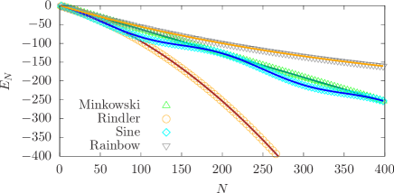
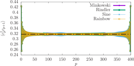
Figure 3: Top: Check of the bulk prediction for the energy, $E_{0}\approx-c_{0}S_{N}$ for four metrics: Minkowski, Rindler ($a=0.01$), Sine ($A=0.5$, $k=\pi/100$) and Rainbow ($h=5\cdot 10^{-3}$. Numerical values are given in dots, while the theoretical prediction is provided in the full line. Bottom: Illustration of the correlator rigidity. Local correlators, $\langle c^{\dagger}_{p}c_{p+1}\rangle$ as a function of the position $p$ for the same four metrics.

The first salient feature of Fig. 4 is that the potential energy $V(p)$ resembles the hopping function $J(x)$, with some strong parity oscillations. We are thus led to conjecture that a classical particle moving on a static metric in (1+1)D would be dragged by a force similar to the graviational pull. Making use of Hellmann-Feynman’s theorem, we see that

$$V(p)\approx-2J_{p}\textrm{Re}\left<c^{\dagger}_{p}c_{p+1}\right>\approx-2J_{p}c_{0}.$$ (22)

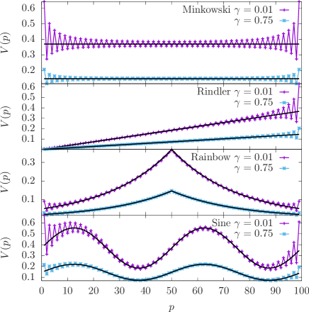
Figure 4: Potential energy $V(p)$ obtained by inhibiting the $p$-th hopping by a factor $\gamma$, $J_{p}\to\gamma J_{p}$, for four different metrics: Minkowski, Rindler ($a=0.01$), rainbow ($h=0.04$) and sinusoidal ($A=0.5$ and $k=2\pi/50$), always using $N=100$ and two values of $\gamma=0.01$ and $0.75$. In continuous line, we plot $J(x)$ mutiplied by a factor which only depends on $\gamma$.

III.2 Finite-Size Corrections

The GS of a finite open chain of $N$ sites in Minkowski spacetime is given by Cardy’s expression Cardy.84 ; Cardy.86 ; DiFrancesco ; Mussardo

$$E_{N}=-c_{0}(N-1)-c_{B}-\dfrac{c\pi v_{F}}{24N}+O(N^{-2}),$$ (23)

where $c$ is the associated central charge, $v_{F}$ is the Fermi velocity and $c_{0}$ and $c_{B}$ are non-universal constants, which correspond to the bulk energy per link and the boundary energy. Notice that the last term is universal, since its form is fixed by conformal invariance Cardy.84 ; Cardy.86 ; DiFrancesco ; Mussardo , but the bulk and boundary terms are not. The GS energy of Hamiltonian (1) with $J_{n}=1$ follows Eq. (23) very accurately, using $c=1$ for Dirac fermions, $v_{F}=2$, $c_{0}=2/\pi$ and $c_{B}=4/\pi-1$.

Our main target is to generalize expression (23) to the case of deformed backgrounds. Indeed, we may follow the guidelines of Sec. II.2 and attempt a substitution $x\to\tilde{x}$, such that $d\tilde{x}/dx=J(x)^{-1}$, but it will not work for the bulk and boundary terms. In that case, the bulk energy would become proportional to $\tilde{N}$. Thus, in the rainbow case we should obtain an energy term which grows exponentially with $N$ for any fixed $h>0$, which is not found. Indeed, as we will show, that transformation is only relevant for the universal term.

Let us propose an extension of Eq. (23) to curved backgrounds based on physical arguments, term by term.

• The term $c_{0}(N-1)$ stands for the bulk energy, which should be replaced by $c_{0}S_{N}$, i.e. the sum of the $N-1$ first hopping amplitudes, multiplied by the local correlator term.

• The boundary term, $c_{B}$ should be proportional to the terminal hoppings, thus generalizing to $c_{B}(J_{1}+J_{N-1})/2$.

• The conformal correction is universal. Thus, it must be naturally deformed, changing $N^{-1}$ into $\tilde{N}^{-1}$, where $\tilde{N}$ is the effective length in deformed coordinates, given by $\tilde{N}=\sum_{i=1}^{N-1}J_{i}^{-1}$ (we let $\Delta x=1$).

Thus, we claim that the correct generalization of Eq. (23) to curved optical lattices is given by

$$E_{N}=-c_{0}S_{N}-{c_{B}\over 2}\left(J_{1}+J_{N-1}\right)-\dfrac{c\pi v_{F}}{24\tilde{N}}+O(N^{-2}).$$ (24)

This expression can be more rigorously justified through a careful analysis of the conformal field theory origin of Eq. (23), and this is discussed in Appendix A.

The inverse of the deformed length $\tilde{N}^{-1}$ can be given an interesting physical interpretation. Indeed, it is easy to recognize $(N-1)\tilde{N}^{-1}$ as the harmonic average of the local speeds of light, which can be understood as an effective Fermi velocity, $\bar{v}_{F}$. Yet, for small deformations, the harmonic average is similar (and lower than) the arithmetical average. Thus, for the sake of simplicity, we approximate $\bar{v}_{F}\approx 2S_{N}/(N-1)$. Thus, we may provide an approximate version of Eq. (24) for a weakly deformed (1+1)D lattice,

$$E_{N}\approx-c_{0}S_{N}-{c_{B}\over 2}(J_{1}+J_{N-1})-{\pi S_{N}\over 12N^{2}}.$$ (25)

III.3 Universality of Casimir forces in curved backgrounds

Numerical checks of Eqs. (24) or (25) must be subtle, because the finite-size correction is typically much smaller than the bulk energy term. Let us consider an alternative observable: the Casimir force measured by a local observer located at the boundary. Since energy is associated to a frequency, local energy measurements at site $x$ will be given by

$$E(x)={E_{N}\over g_{00}^{1/2}(x)}={E_{N}\over J_{N}}.$$ (26)

Such an observer will measure a force given by the covariant spatial derivative of $F=-D_{x}E(x)$, taking the lattice spacing $\Delta x=1$ (see Appendix B for details) and changing the sign for convenience, we define

$$F_{N}\equiv{E_{N}-E_{N-2}\over J_{N-1}+J_{N-2}}.$$ (27)

Assuming smoothly varying hopping amplitudes we obtain

$$F_{N}\equiv-c_{0}-{c_{B}\over 2}\left({J^{\prime}_{N}\over J_{N}}\right)-{\pi\over 12N^{2}}+{\pi S_{N}\over 6J_{N}N^{3}}.$$ (28)

Let us consider the terms individually. The first, $c_{0}=2/\pi$, is simply associated to the bulk energy. The second is a boundary force, which is absent from the homogeneous case, and will take a leading role in some cases. For very weak deformations, $J_{N}\approx J_{0}+\delta J_{N}$ is a small deformation, we can assume that $S_{N}\approx NJ_{N}$, and we obtain

$$F_{N}\approx-c_{0}-{c_{B}\over 2}\left({J^{\prime}_{N}\over J_{N}}\right)+{\pi\over 12N^{2}}.$$ (29)

Thus, we are led to the following claim: Casimir forces on a weakly curved background are metric-independent when measured by a local observer at the boundary. Indeed, consider an observer on a classical obstacle located at site $p$. It will be subject both to a left and a right Casimir forces. The bulk and boundary parts will cancel out, and only the universal finite-size correction will survive, yielding

$$F(p)=F_{N-p}-F_{p}={\pi\over 12}\left({1\over(N-p)^{2}}-{1\over p^{2}}\right).$$ (30)

The validity of expression (29) can be checked in Fig. 5. In all cases, the black continuous line is the theoretical prediction, Eq. (29). The top panel shows the forces $F_{N}+c_{0}$ as a function of $N$ for Rindler metrics of different sizes, varying both $J_{0}$ and the acceleration $a$. We have included the Minkowski case, which corresponds to $J_{0}=1$ and $a=0$, as one of the limits. We notice that $F_{N}+c_{0}$ can be both positive and negative, depending on the values of $J_{0}$ and the acceleration $a$. This behavior is explained through our expression (29): the boundary term scales like $N^{-1}$ and it is always negative. Meanwhile, the universal conformal term scales like $N^{-2}$ and is always positive. Thus, the prevalence of one or the other explains the global behavior, but for large enough $N$ the boundary term is always dominant. This trade-off can be visualized in the inset, where we plot the absolute value $|F_{N}+c_{0}|$ as a function of $N$ in log-log scale. For Minkowski, $J_{0}=1$ and $a=0$, the $1/N^{2}$ behavior extends for all sizes, but as soon as $a>0$ we observe a small-$N$ behavior like $N^{-2}$ which performs a crossover into the dominant $N^{-1}$ term beyond a finite size which scales as $(J_{0}/a)^{1/2}$.

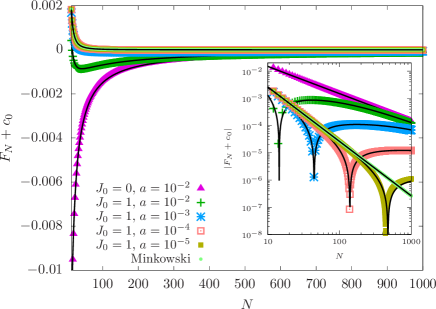
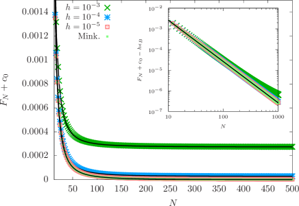
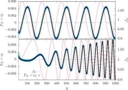
Figure 5: Casimir forces, $F_{N}+c_{0}$, for different metrics. Top: Rindler metric. Inset, log-log plot of $|F_{N}+c_{0}|$ as a function of $N$, in log-log scale. Notice most small systems are dominated by the CFT correction, while for larger sizes the boundary term $N^{-1}$ dominates. Center: Rainbow metric, we observe that $F+c_{0}$ tends to $\epsilon_{B}h$. Inset: log-log plot of $F_{N}+c_{0}-\epsilon_{B}h$. Bottom: Sinusoidal metric (top) and modulated frequency metric (bottom).

The central panel of Fig. 5 shows the case of the Casimir forces in the rainbow state, for which the boundary term is constant: $J^{\prime}_{N}/J_{N}=-h$ for all $N$. Thus, the behavior of $F_{N}+c_{0}$ corresponds merely to the CFT term, Eq. (23) with a constant additive correction. This behavior is further clarified when this constant is removed, and we observe the nearly perfect collapse of all the forces in the inset of Fig. 5 (center).

We have also considered is the sinusoidal metric, Eq. (6), where the boundary term dominates the force for large $N$, while the CFT term dominates for low $N$, as we can see in the bottom panel of Fig. 5. There, we can observe the behavior of the hoppings (in pale pink), along with the forces and their fit to expression (29). Indeed, the force behaves like the derivative of the hopping function. In order to highlight this behavior, we have considered yet another metric, given by

$$J_{N}=1+A\sin(kN^{2}),$$ (31)

i.e. a modulated frequency sinusoidal. The results are shown in the bottom panel of Fig. 5, showing again an excellent agreement between the theory and the numerical experiments.

IV Casimir force in the inhomogeneous Heisenberg model

We may wonder whether these results are only valid for free fermions or if, instead, they can be applied to other CFT. Thus, we have considered one of the simplest critical interacting systems, the (inhomogenous) spin-1/2 Heisenberg model in 1D, defined by

$$H=-\sum_{i=1}^{L-1}J_{i}\;\vec{S}_{i}\cdot\vec{S}_{i+1},$$ (32)

Using the Jordan-Wigner transformation we may rewrite it in fermionic language as

$$H=-\sum_{i=1}^{L-1}J_{i}\left(c^{\dagger}_{i}c_{i+1}+\text{h.c.}\right)+2\sum_{i=1}^{L}J_{i}\,n_{i}n_{i+1},$$ (33)

where we can see that fermionic particles at nearby sites repel each other, making it impossible to use free-fermion techniques. Yet, the GS energy of this Hamiltonian can be accurately obtained using the density matrix renormalization group (DMRG) algorithm White_92 ; White_93 ; Details . The results for the Rindler couplings, Eq. (5) are shown in Fig. 6. The maximal size that we have reached is lower than in the previous case, $N=100$, because the numerical computation is more demanding. Yet, the results show that a straightforward extension of Eq. (29) predicts the force values with a remarkable accuracy using $c_{0}=0.4431$, $c_{B}=0.2618$ and $v_{F}=1.319$, through

$$F_{N}\approx-c_{0}-{c_{B}\over 2}\left({J^{\prime}_{N}\over J_{N}}\right)+{\pi v_{F}\over 24N^{2}}.$$ (34)

Fig. 6 shows $|F_{N}+c_{0}|$ in logarithmic scale as a function of $N$ for different Rindler deformations of the Heisenberg Hamiltonian, along with the theoretical prediction, Eq. (29). These plots can be compared with the inset of Fig. 5 (top).

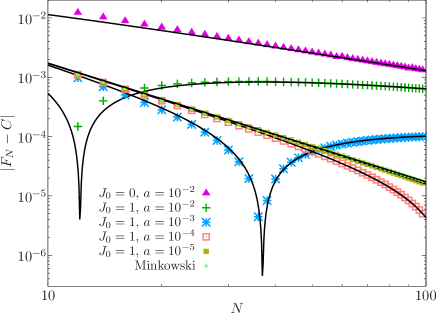
Figure 6: Casimir forces for the spin-1/2 Heisenberg chain with Rindler couplings. The black lines correspond to the theoretical prediction, given by Eq. (34). Compare to the inset of Fig. 5 (top).

V Conclusions and further work

We have derived an expression for the ground-state energy of the discretized version of the Dirac equation in a deformed (1+1)D medium, which corresponds to the vacuum state in static curved metrics. We can model a classical particle navigating through the system depressing a local hopping, and then it can be readily checked that the classical particle moves approximately in a potential which corresponds to the classical gravitational potential associated with the metric. The quantum corrections to this semi-classical result can be obtained by suitably deforming the predictions of conformal field theory (CFT). Indeed, we have checked that the finite-size corrections are dominated by two terms: a boundary term related to the derivative of the local hopping amplitude at the edge of the system, and a naturally deformed version of the CFT force, where the central charge is preserved. The conformal correction can be interpreted in two complementary ways: either the Fermi velocity is substituted by the (harmonic) average value of the hopping terms, or the system size is transformed by its deformed value.

In any case, we should emphasize that the finite-size corrections to the vacuum energy are, indeed, universal. Moroever, we have shown that an observer at a boundary measuring the Casimir forces will obtain a metric-independent value.

It is relevant to ask whether our results extend to other conformal field theories, both interacting, such as Heisenberg, or non-interacting, such as the Ising model in a transverse field. Even more challenging will be to extend these results to (2+1)D field theories and to consider non-static metrics, where the dynamical effects will be relevant, linking them to the dynamical Casimir effect Nation.12 . Even if the energy is not defined in those cases, a force can still be found acting on classical particles. It is also interesting to consider chains under strong inhomogeneity or randomness Ramirez.random.14 ; Laguna.16 ; Alba.19 ; Samos.19b .

As a natural next step, we intend also to develop protocols in order to confirm these results in the laboratory employing ultra-cold atoms in optical lattices, where similar curved-metric problems have been addressed in the past, such as the measurement of the Unruh effect Boada.11 ; Laguna_unruh.17 .

Appendix A CFT derivation of the Casimir energy in curved backgrounds

Let us provide a theoretical justification for our deformed extension of expression (23), given in Eq. (24). The two first terms are non-universal: $c_{0}(N-1)\mapsto c_{0}S_{N}$, while $c_{B}\mapsto(c_{B}/2)(J_{1}+J_{N})$ are just a consequence of first-order perturbation theory. Yet, the finite-size correction term ($c\pi v_{F}/24N$) is universal, i.e. fixed by conformal invariance, and requires further explanation. In what follows we will assume that the Fermi velocity (the speed of light) is $v_{F}=1$.

According to CFT, the variation of the energy-momentum tensor $T$ under a local conformal transformation, $z\rightarrow w(z)$, in flat spacetime is given by DiFrancesco

$$T^{\prime}(w)=\left(\dfrac{dw}{dz}\right)^{-2}\left[T(z)-\dfrac{c}{12}\{w;z\}\right],$$ (35)

where $c$ is the central charge of the CFT and $\{w;z\}$ is the Schwarzian derivative,

$$\{w;z\}=\dfrac{d^{3}w/dz^{3}}{dw/dz}-\dfrac{3}{2}\left(\dfrac{d^{2}w/dz^{2}}{dw/dz}\right)^{2}.$$ (36)

Let us consider a CFT defined on the whole complex plane, with vanishing energy density $\left<T(z)\right>\sim 0$. Now, we would like to map it into a strip of width $L$, using

$$z\rightarrow w=\dfrac{L}{\pi}\ln{z}.$$ (37)

This yields a nonzero vacuum energy density on the strip

$$\left<T_{\text{strip}}(w)\right>=-\dfrac{c\pi^{2}}{24\,L^{2}}.$$ (38)

Now, the energy density can be evaluated (check Eq. (5.40) of DiFrancesco ),

$$\left<T^{00}\right>=\left<T_{zz}\right>+\left<T_{\bar{z}\bar{z}}\right>=-{1\over\pi}\left<T\right>={\pi c\over 24L^{2}},$$ (39)

which corresponds to the universal term in Eq. (23). Yet, our $z$ variable is composed of a deformed space variable and time, $z=\tilde{x}+it$, so the length appearing in this expression is, in fact, $\tilde{L}$, as required.

Let us provide an alternative derivation, only valid for infinitesimal deformations of the metric, $g_{\mu\nu}\mapsto g_{\mu\nu}+\delta g_{\mu\nu}$. The free energy density of a conformal system, $F$, varies as

$$\delta F=-\dfrac{1}{2}\int d^{2}x\;\sqrt{g}\;\delta g_{\mu\nu}\left<T^{\mu\nu}\right>,$$ (40)

where $\sqrt{g}=\det\left(g_{\mu\nu}\right)^{1/2}$ is required by the invariance of the spacetime integration measure. Let consider the Minkowski energy density, given by

$$T^{00}=\dfrac{\pi c}{24\,L^{2}},$$ (41)

and deform the metric, mapping $g_{00}=-1$ to $g_{00}+\delta g_{00}=-J^{2}(x)\approx-1-2\delta J(x)$. This leads to a new free energy,

$$\delta F=\int d^{2}x\;\delta J(x){\pi c\over 24\,L^{2}},$$ (42)

where the integration must be performed on a strip $[0,L]\times{\mathbb{R}}$, where the vertical direction is trivial. The total energy is given by the new free energy per unit length (in the transverse direction),

$$E=F_{L}+\delta F_{L}=\left({1\over L}\int_{0}^{L}dx\,(1+\delta J(x))\right){\pi c\over 24\,L},$$ (43)

i.e. the energy gets corrected by a new Fermi velocity, which is equal to the average value of $J(x)$ in the interval. This is the main result of Eq. (25).

Of course, this result is only valid for very small deformations, $J(x)\approx 1+\delta J(x)$. The full expression (24) can be obtained by integrating it, $F=\int\delta F$. We may parametrize the change from $g_{00}=-1$ to $g_{00}=-J^{2}(x)$ in a continuous way, considering a one-parameter metric family, $g_{00}(s)=J^{2}(x,s)$ such that $J^{2}(x,0)=-1$ and $J^{2}(x,1)=J^{2}(x)$, so that the final energy correction takes the form

$$\Delta F=\int_{0}^{1}ds\int dx\sqrt{g(s)}\left(\dfrac{\pi c}{24L(s)^{2}}\right){\partial J(x,s)\over\partial s},$$ (44)

where $L(s)$ and $\sqrt{g(s)}$ correspond respectively to the effective length and the volume factor at each stage of the deformation process.

Appendix B Casimir force measured by local observer

Let $E$ be the Casimir energy for the whole system. When it is measured by a local observer at site $x$ will be given by $E(x)=E/g_{00}(x)^{1/2}=E/J(x)$, following Eq. (26). Let us remember that the energy is not a scalar, but a vector pointing along the time axis: $(E(x),0)$. The force is defined as the spatial component of the covariant derivative of the energy,

$$F(x)=-D_{x}E(x),$$ (45)

where the covariant derivative of a vector is defined as

$$D_{\mu}V^{\alpha}=\partial_{\mu}V^{\alpha}+\Gamma^{\alpha}_{\mu\nu}V^{\nu},$$ (46)

where the $\Gamma^{\alpha}_{\mu\nu}$ are the Christoffel symbols, given by

$$\Gamma^{\alpha}_{\mu\nu}={1\over 2}g^{\alpha\beta}\left(g_{\beta\mu,\nu}+g_{\beta\nu,\mu}-g_{\mu\nu,\beta}\right).$$ (47)

for the metric connection. In the case of an optical metric, Eq. (2), the only relevant Christoffel symbol is

$$\Gamma^{0}_{10}={J^{\prime}(x)\over J(x)}.$$ (48)

Thus, we can find the force

$$F(x)=-{\partial_{x}E(x)\over J(x)}+{J^{\prime}(x)\over J(x)}E(x)-{J^{\prime}(x)\over J(x)}E(x)=-{\partial_{x}E(x)\over J(x)}.$$ (49)

And from this equation we can find a possible definition of the Casimir force felt by a local observer at the boundary,

$$F_{N}\approx-{E_{N}-E_{N-1}\over J_{N}\Delta x},$$ (50)

where we set $\Delta x=1$, since it is arbitrary. Yet, the strong parity oscillations suggest that a better alternative is to take the discrete derivative over two lattice spacings,

$$F_{N}\equiv-{E_{N}-E_{N-2}\over J_{N-2}+J_{N-1}}.$$ (51)

References

- (1) HBG Casimir, D Polder, The Influence of Retardation on the London-van der Waals Forces, Phys. Rev. 73, 360 (1948).
- (2) GL Klimchitskaya, VM Mostepanenko, Experiment and theory in the Casimir effect, Contemp. Phys. 47, 131 (2006).
- (3) M Kardar, R Golestanian, The friction of vacuum, and other fluctuation-induced forces, Rev. Mod. Phys. 71, 1233 (1999).
- (4) O Kenneth, Israel Klich, Opposites Attract: A Theorem about the Casimir Force, Phys. Rev. Lett. 97, 160401 (2006).
- (5) M Asorey, JM Muñoz-Castañeda, Attractive and repulsive Casimir vacuum energy with general boundary conditions, Nucl. Phys. B 874, 852 (2013).
- (6) P Sundberg, RL Jaffe, The Casimir effect for fermions in one dimension, Ann. Phys. 309, 442 (2004).
- (7) D Zhabinskaya, JM Kinder, EJ Mele, Casimir effect for massless fermions in one dimension: A force-operator approach, Phys. Rev. A 78, 060103 (2008).
- (8) JL Cardy, Conformal invariance and universality in finite-size scaling, J. Phys. A: Math. Gen. 17, L385 (1984).
- (9) HWJ Blöte, JL Cardy, MP Nightingale, Conformal Invariance, the Central Charge, and the Universal Finite-Size Amplitudes at Criticality, Phys. Rev. Lett. 56, 742 (1986).
- (10) P di Francesco, P Matthieu, D Sénéchal, Conformal Field Theory, Springer (1997).
- (11) G. Mussardo, Statistical Field Theory, Oxford Graduate Texts (2010).
- (12) G Bimonte, T Emig, M Kardar, Conformal field theory of critical Casimir interactions in 2D, EPL 104, 21001 (2013).
- (13) B DeWitt, Quantum field theory in curved spacetime, Phys. Rep. 19, 295 (1975).
- (14) F Sorge, Casimir effect in a weak gravitational field, Class. Quantum Grav. 22, 5109 (2005).
- (15) F Sorge, Casimir effect in weak gravitational field: Schwinger’s approach,
- (16) M Nouri-Zonoz, B Nazari, Vacuum energy and the spacetime index of refraction: A new synthesis, Phys. Rev. D 82, 044047 (2010).
- (17) B Nazari, M Nouri-Zonoz, Electromagnetic Casimir effect and the spacetime index of refraction, Phys. Rev. D 85, 044060 (2012).
- (18) U Leonhardt, Lifshitz theory of the cosmological constant, Ann. Phys. 411, 167973 (2019).
- (19) U Leonhardt, The case for a Casimir cosmology, Phil. Trans. R. Soc. A 378, 20190229 (2020).
- (20) M Lewenstein, A Sanpera, V Ahufinger, Ultracold atoms in optical lattices, Oxford University Press (2012).
- (21) O Boada, A Celi, JI Latorre, M Lewenstein, Dirac equation for cold atoms in artificial curved spacetimes, New J. Phys. 13, 035002 (2011).
- (22) J Rodríguez-Laguna, L Tarruell, M Lewenstein, A Celi, Synthetic Unruh effect in cold atoms, Phys. Rev. A 95, 013627 (2017).
- (23) S Takagi, Vacuum noise and stress induced by uniform acceleration, Prog. Theor. Phys. Supp. 88, 1 (1986).
- (24) J Louko, Thermality from a Rindler quench, Class. Quant. Grav. 35 205006 (2018).
- (25) J Eisert, M Cramer, MB Plenio, Colloquium: Area laws for the entanglement entropy, Rev. Mod. Phys. 82, 277 (2010).
- (26) G Vitagliano, A Riera, JI Latorre, Volume-law scaling for the entanglement entropy in spin-1/2 chains, New J. of Phys. 12, 113049 (2010).
- (27) G Ramirez, J Rodriguez-Laguna, G Sierra, From conformal to volume-law for the entanglement entropy in exponentially deformed critical spin 1/2 chains, JSTAT P10004 (2014).
- (28) G Ramirez, J Rodriguez-Laguna, G Sierra, Entanglement over the rainbow, JSTAT P06002 (2015).
- (29) C Holzhey, F Larsen, F Wilczek, Geometric and renormalized entropy in conformal field theory, Nucl. Phys. B 424, 443 (1994).
- (30) G Vidal, JI Latorre, E Rico, A Kitaev, Entanglement in quantum critical phenomena, Phys. Rev. Lett. 90 227902 (2003).
- (31) P Calabrese, JL Cardy, Entanglement entropy and quantum field theory, JSTAT P06002 (2004).
- (32) P Calabrese, J Cardy, Entanglement entropy and conformal field theory, J. Phys. A 42, 504005 (2009).
- (33) J Rodríguez-Laguna, J Dubaîl, G Ramírez, P Calabrese, G Sierra, More on the rainbow chain: entanglement, space-time geometry and thermal states, J. Phys. A 50, 164001 (2017).
- (34) E Tonni, J Rodríguez-Laguna, G Sierra, Entanglement hamiltonian and entanglement contour in inhomogeneous 1D critical systems, JSTAT 043105 (2018).
- (35) I MacCormack, AL Liu, M Nozaki, S Ryu, Holographic Duals of Inhomogeneous Systems: The Rainbow Chain and the Sine-Square Deformation Model, J. Phys. A: Math. and Theor. 52, 505401 (2019).
- (36) RM Wald, General relativity, The University of Chicago Press (1984).
- (37) B-Q Jin, VE Korepin, Quantum Spin Chain, Toeplitz Determinants and the Fisher—Hartwig Conjecture, J. Stat. Phys. 116, 79 (2004).
- (38) M Fagotti, P Calabrese, JE Moore, Entanglement spectrum of random-singlet quantum critical points, Phys. Rev. B 83, 045110 (2011).
- (39) SR White, Density matrix formulation for quantum renormalization groups, Phys. Rev. Lett. 69, 2863 (1992).
- (40) SR White, Density matrix algorithms for quantum renormalization groups, Phys. Rev. B 48, 10345 (1993).
- (41) We employ the finite-size DMRG algorithm with preservation, with an adaptive number of retained states so that the discarded weight in the density matrix is always under .
- (42) PD Nation, JR Johansson, MP Blencowe, F Nori, Stimulating uncertainty: Amplifying the quantum vacuum with superconducting circuits, Rev. Mod. Phys. 84, 1 (2012).
- (43) G Ramírez, J Rodríguez-Laguna, G Sierra, Entanglement in low-energy states of the random-hopping model, JSTAT P07003 (2014).
- (44) J Rodríguez-Laguna, SN Santalla, G Ramírez, G Sierra, Entanglement in correlated random spin-chains, RNA folding and kinetic roughening, New J. Phys. 18, 073025 (2016).
- (45) V Alba, SN Santalla, P Ruggiero, J Rodríguez-Laguna, P Calabrese, G Sierra, Unusual area-law violation in random inhomogeneous systems, JSTAT 023105 (2019).
- (46) N. Samos Sáenz de Buruaga, S.N. Santalla, J. Rodríguez-Laguna, G. Sierra, Piercing the rainbow: entanglement on an inhomogeneous spin chain with a defect, Phys. Rev. B 101, 205121 (2020).
- (47) I. Peschel, Calculation of reduced density matrices from correlation functions, J. Phys. A: Math. Gen. 36, L205 (2003).