Engineering Dynamical Sweet Spots to Protect Qubits from 1/$f$ Noise

Abstract

Protecting superconducting qubits from low-frequency noise is essential for advancing superconducting quantum computation. Based on the application of a periodic drive field, we develop a protocol for engineering dynamical sweet spots which reduce the susceptibility of a qubit to low-frequency noise. Using the framework of Floquet theory, we prove rigorously that there are manifolds of dynamical sweet spots marked by extrema in the quasi-energy differences of the driven qubit. In particular, for the example of fluxonium biased slightly away from half a flux quantum, we predict an enhancement of pure-dephasing by three orders of magnitude. Employing the Floquet eigenstates as the computational basis, we show that high-fidelity single- and two-qubit gates can be implemented while maintaining dynamical sweet-spot operation. We further confirm that qubit readout can be performed by adiabatically mapping the Floquet states back to the static qubit states, and subsequently applying standard measurement techniques. Our work provides an intuitive tool to encode quantum information in robust, time-dependent states, and may be extended to alternative architectures for quantum information processing.

I Introduction

Low-frequency noise has been a limiting factor for dephasing times of many solid-state based qubits [1, 2, 3, 4, 5, 6, 7, 8, 9, 10, 11, 12, 13, 14, 15, 16, 17, 18, 19, 20, 21, 22, 23, 24, 25, 26, 27, 28, 29, 30, 31, 32, 33, 34, 35, 36]. Superconducting qubits especially suffer from 1/$f$ charge and flux noise [1, 2, 3, 4, 5, 6, 10, 11, 12, 13, 7, 14, 8, 15, 16, 17, 18, 9, 19, 21, 20, 22]. A conventional way to improve dephasing times is to operate the qubit at so-called sweet spots [5, 6, 7, 8, 9]. These sweet spots correspond to extrema of the qubit’s transition frequency [5], see Fig. 1(a) for an example. Another established method for improving dephasing times is dynamical-decoupling (DD) [18, 37, 38, 39, 40, 41], which is well-known in the context of NMR echo sequences [42, 43, 44], and has been successfully applied to superconducting qubits [18, 38].

In this paper, we propose a qubit protection protocol based on dynamical sweet spots [20, 21, 22, 19, 23, 24]. Inspired by static sweet-spot operation and dynamical decoupling, this protocol employs a periodic drive to mitigate the dephasing usually induced by $1/f$ noise. Utilizing Floquet theory, we show that dynamical sweet spots represent extrema in the qubit’s quasi-energy difference, and thus generalize the concept of static sweet spots [Fig. 1(b)]. Notably, dynamical sweet spots are generally not isolated points, but rather form extended sweet-spot manifolds in parameter space. The multi-dimensional nature of dynamical sweet spots provides additional freedom to tune qubit properties such as the transition frequency while maintaining dynamical protection. We show that dynamical sweet-spot operation can simultaneously yield both long depolarization ($T_{1}$) and pure-dephasing times ($T_{\phi}$).

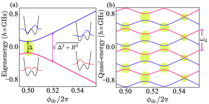
Figure 1: (a) Static fluxonium spectrum as a function of magnetic flux. Insets show the qubit eigenfunctions at the sweet spot and slightly away from it ($\phi_{\mathrm{dc}}/2\pi=0.52$). The parameters used are: $E_{\mathrm{C}}/h=0.5\,\text{GHz}$, $E_{\mathrm{J}}/h=4.0\,\text{GHz}$ and $E_{\mathrm{L}}/h=1.3\,\text{GHz}$ for the capacitive, Josephson and inductive energy, respectively. (b) Quasi-energy spectrum of the driven qubit for flux $\phi_{\mathrm{ac}}/2\pi=0.028$ and drive frequency $\omega_{\mathrm{d}}/2\pi=490\,$MHz. The highlighted regions in both panels mark the flux sweet spots. The drive produces numerous dynamical sweet spots at different dc flux values, as opposed to only one in the static case.

This protection scheme can also be interpreted as a continuous version of DD [45]. Here, the sequences of ultra-short pulses widely used in many DD experiments are replaced by a periodic drive on the qubit, which is much easier to realize experimentally. In addition to earlier explorations in this direction [5, 23, 46, 47, 48, 49, 27, 24, 26, 25, 20, 21, 22, 19], we here provide a systematic and general framework for locating dynamical sweet-spot manifolds in the control parameter space. This framework is general enough to cover a variety of qubit systems beyond the specific example discussed here, and can be adapted to different types of drives as well as noise environments. Indeed, some of the previously developed protection schemes [5, 19, 20, 21, 22, 46, 47, 23, 48, 49] based on qubit-frequency modulation or on-resonant Rabi drives, can be understood as special limits of the framework presented here (see Supplemental Material [50] for details). The theoretical approach we develop allows us not only to predict the improvement of pure-dephasing times, but also to assess how dynamical depolarization times are affected by the driving. We further show that the protection scheme is compatible with concurrent single- and two-qubit gate operations, thus making it suitable for both quantum information storage and processing. In a companion experimental paper [51], our theoretical results are demonstrated to lead to a significant improvement in the dephasing time of a flux-modulated fluxonium qubit.

The paper is structured as follows. Throughout this paper, we consider the superconducting fluxonium qubit [52, 53, 17, 54, 13, 12, 7, 8, 34, 14] a platform for illustrating the dynamical-protection protocol. We begin in Section II, with a description of this qubit and discuss its static coherence times in the absence of external driving. In Section III, we employ Floquet theory to derive expressions for the dynamical coherence times of the driven qubit. We then evaluate these expressions numerically in Section IV, and discuss the nature of the observed dynamical sweet spots associated with increases in coherence times. We illustrate how to perform gate operations and readout on such a driven qubit (Floquet qubit) in Section V, and further show how to implement a Floquet two-qubit gate in Section VI. Finally, we present our conclusions in Section VII.

II Two-level system subject to $\mathbf{1/f}$ noise

For concreteness, we discuss the application of the protection scheme to the most recent genereation of fluxonium qubits [52, 53, 17, 54, 13, 12, 7, 8, 34, 14], though the general theoretical framework is not limited to this choice. Fluxonium qubits biased close to half-integer flux exhibit attractive properties including increased coherence times as compared to other superconducting qubits [13, 12, 7, 8, 51, 53]. When the external flux bias in the circuit loop is tuned to the sweet spot at half a flux quantum, both depolarization and dephasing times of the fluxonium circuit exceed 100$\,\mu$s and is strongly anharmonic [7, 8, 51]. However, this sweet spot is point-like, and the qubit regains sensitivity to 1/$f$ flux noise when the external flux is tuned slightly away from the half-integer point [12, 13, 7, 8, 17, 14]. This sensitivity leads to increased pure dephasing of the fluxonium qubit. We note that in multi-loop circuits with shared inductance, the local nature of 1/$f$ flux noise produces further constraints on the existence of static flux sweet spots [17]. It is thus desirable to find alternative means of protection from 1/$f$ flux noise, in order to improve coherence times, and advance the promising direction of quantum-information processing with fluxonium qubits.

Our protection scheme is based on introducing a modulation of the external flux close to the static sweet spot, i.e., $\phi_{\text{ext}}(t)=\phi_{\mathrm{ac}}\cos(\omega_{\mathrm{d}}t)+\phi_{\mathrm{dc}}$. Here, $\phi_{\mathrm{ext}}=2\pi\Phi_{\text{ext}}/\Phi_{0}$ denotes the reduced external flux, $\Phi_{0}$ is the flux quantum, and $\phi_{\mathrm{ac}}$, $\phi_{\mathrm{dc}}$ are its ac modulation amplitude and dc offset, respectively. Upon truncation to two levels, the effective Hamiltonian of the driven fluxonium circuit is given by

$$\hat{H}_{\mathrm{q}}(t)=\frac{\Delta}{2}\hat{\sigma}_{x}+\left(A\cos\omega_{\mathrm{d}}t+\frac{B}{2}\right)\hat{\sigma}_{z},$$ (1)

see Appendix A for details. Here, $\Delta$ denotes the qubit splitting at $\phi_{\mathrm{dc}}=\pi$, and $A\propto\phi_{\mathrm{ac}}$ and $B\propto\delta\phi_{\mathrm{dc}}=\phi_{\mathrm{dc}}-\pi$ are the effective drive amplitude and dc bias away from the static sweet spot. Note that we also set $\hbar=1$ in this expression. The resulting eigenenergies of the static qubit ($\phi_{\mathrm{ac}}=0$) are plotted in Fig. 1(a) as a function of $\phi_{\mathrm{dc}}$. The full Hamiltonian including the qubit-bath coupling is given by $\hat{H}=\hat{H}_{\mathrm{q}}(t)+\hat{H}_{\mathrm{B}}+\hat{H}_{\mathrm{int}}$, where $H_{\mathrm{B}}$ and $H_{\mathrm{int}}$ denote the Hamiltonian of the bath and the qubit-bath interaction. We consider two major noise sources that often limit fluxonium coherence times: 1/$f$ flux noise and dielectric loss [13, 7, 14, 15, 8, 16]. The corresponding interaction Hamiltonian thus takes the form $\hat{H}_{\text{int}}=(\hat{\eta}_{\mathrm{f}}+\hat{\eta}_{\mathrm{d}})\hat{\sigma}_{z}$, where $\hat{\eta}_{\mathrm{f}}$ and $\hat{\eta}_{\mathrm{d}}$ are the bath operators through which 1/$f$ flux noise and dielectric loss are induced. The noise spectra characterizing these channels are given by $S_{\mathrm{f}}(\omega)=\mathcal{A}^{2}_{\mathrm{f}}|\omega/2\pi|^{-1}$ and $S_{\mathrm{d}}(\omega)=\alpha(\omega,T)\mathcal{A}_{\mathrm{d}}(\omega/2\pi)^{2}$ [55]. Here, $\alpha(\omega,T)=|\coth(\omega/2k_{\mathrm{B}}T)+1|/2$ is a thermal factor, $k_{\mathrm{B}}$ and $T$ denote the Boltzmann constant and temperature, and $\mathcal{A}_{\mathrm{f}}$ and $\mathcal{A}_{\mathrm{d}}$ denote the noise amplitudes.

As reference for our discussion of dynamical coherence times in Secs. III and IV, we first briefly review the static coherence times of the undriven qubit. The decoherence rates depend on the matrix elements of the qubit operator coupling to the noise as well as the noise spectra. For a non-singular noise spectrum $S(\omega)$, the rates for relaxation, excitation and pure dephasing are

$$\gamma_{\mp}= \,|\sigma_{z}^{ge}|^{2}\,S(\pm\Omega_{ge}),$$ (2)

$$\gamma_{\phi}= \,|\sigma_{z}^{ee}-\sigma_{z}^{gg}|^{2}\,S(0)/2.$$ (3)

As usual, these expressions are derived within Bloch-Redfield theory. Here, $|g\rangle$ and $|e\rangle$ denote the qubit ground and first excited state, $\Omega_{ge}=\sqrt{\Delta^{2}+B^{2}}$ the corresponding eigenenergy difference, and $\sigma_{z}^{ll^{\prime}}\equiv\langle l|\hat{\sigma}_{z}|l^{\prime}\rangle$ ($l,l^{\prime}=g,e$) the relevant matrix elements. (Since these matrix elements will appear rather frequently, we choose to introduce this slightly more compact notation.) The quantity $|\sigma_{z}^{ee}-\sigma_{z}^{gg}|$ governing the pure-dephasing rate $\gamma_{\phi}$ turns out to be proportional to the flux dispersion of the eigenenergy difference $|\partial\Omega_{ge}/\partial\phi_{\mathrm{dc}}|$, in agreement with the well-known proportionality $\gamma_{\phi}\propto(\partial\Omega_{ge}/\partial\phi_{\mathrm{dc}})^{2}$ [5, 6]. For the realistic noise spectrum $S(\omega)=S_{\mathrm{d}}(\omega)+S_{\mathrm{f}}(\omega)$, however, there is a divergence at $\omega=0$ from the $1/f$ flux noise. In this case, our evaluation of dephasing times includes careful consideration of frequency cutoffs, see Refs. [5, 56, 6, 20].

The resulting coherence times differ characteristically according to the flux bias. Away from the flux sweet spot, the qubit has wavefunctions with disjoint support [insets of Fig. 1(a)]. This leads to a suppression of the coefficient $|\sigma_{z}^{ge}|^{2}$ relevant for relaxation and excitation, and hence to a relatively long depolarization time of $T_{1}=770\,\mu\text{s}$ (see Table 1 caption for our specific choice of parameters). The pure-dephasing time of $T_{\phi}=0.88\,\mu\text{s}$ is rather short, on the other hand, since the flux dispersion $\partial\Omega_{ge}/\partial\phi_{\mathrm{dc}}$ is significant away from the flux sweet spot. At the flux sweet spot, the situation changes: disjointness of eigenfunctions is lost and depolarization times are correspondingly shorter, $T_{1}=360\,\mu$s. Since the flux dispersion $\partial\Omega_{ge}/\partial\phi_{\mathrm{dc}}$ vanishes at the sweet spot, the qubit is less sensitive to 1/$f$ noise, resulting in a pure-dephasing time exceeding $10\,$ms [7, 57], limited only by second-order contributions from 1/$f$ flux noise. In realistic settings, the pure-dephasing times will be limited by other sources including photon shot noise, critical current noise, etc [58, 59, 35, 36].

III Dynamical coherence times of the driven qubit

The analysis of coherence times must be modified when including a periodic drive acting on the qubit. Based on an open-system Floquet theory [60, 61], the coherence times are most conveniently characterized in the basis formed by the qubit’s Floquet states. The quasi-energies $\epsilon_{j}$ and time-periodic Floquet states $|w_{j}(t)\rangle$ of the driven qubit, labeled by index $j$, are the counterparts of the ordinary eigenstates and eigenenergies in the undriven case [62, 63, 64, 61]. They are obtained as solutions of the Floquet equation

$$\left[\hat{H}_{\mathrm{q}}(t)-i\frac{\partial}{\partial t}\right]|w_{j}(t)\rangle=\epsilon_{j}|w_{j}(t)\rangle.$$ (4)

In the absence of noise, the evolution operator $U_{\mathrm{q}}(t,0)=\sum_{j=0,1}|w_{j}(t)\rangle\langle w_{j}(0)|\exp(-i\epsilon_{j}t)$ governs the evolution of the driven qubit. As a result, the population in each Floquet state remains invariant, while the relative phase accumulates at a rate given by the quasi-energy difference $\epsilon_{01}\equiv\epsilon_{1}-\epsilon_{0}$.

The matrix elements and noise frequencies relevant for the decoherence of the driven qubit crucially differ from the undriven case. By casting the expression for the decoherence rates into the form

$$\gamma_{\mu}=\int^{\infty}_{-\infty}F_{\mu}(\omega)S(\omega)\mathrm{d}\omega,$$ (5)

these differences are conveniently captured as a change in the filter function $F_{\mu}(\omega)$ [15, 65]. Here, $\mu=\mp,\phi$ denotes the different noise channels corresponding to relaxation, excitation and pure dephasing.

For the undriven qubit, $F_{\mu}(\omega)$ is strongly peaked at the filter frequencies $\omega=\pm\Omega_{ge}$ and $\omega=0$. The integrated peak areas, referred to as weights, are given by the quantities $|\sigma_{z}^{ge}|^{2}$, $|\sigma_{z}^{eg}|^{2}$ and $|\sigma_{z}^{ee}-\sigma_{z}^{gg}|^{2}/2$ associated with the three noise channels. By contrast, for the driven qubit, $F_{\mu}(\omega)\sim\sum_{k}|g_{k\mu}|^{2}\delta(\omega-\bar{\omega}_{k\mu})$ develops additional sideband peaks, resulting in filter frequencies $\bar{\omega}_{k\mp}=\pm\epsilon_{01}+k\omega_{\mathrm{d}}$ and $\bar{\omega}_{k\phi}=k\omega_{\mathrm{d}}$ ($k\in\mathbb{Z}$). The corresponding weights are $|g_{k\mp}|^{2}$ and $2|g_{k\phi}|^{2}$, where

$$g_{k+}= \frac{\omega_{\mathrm{d}}}{2\pi}\int_{0}^{2\pi/\omega_{\mathrm{d}}}dt\,e^{ik\omega_{\mathrm{d}}t}\,\operatorname{Tr}\left(\sigma_{z}|w_{0}(t)\rangle\langle w_{1}(t)|\right),$$ (6)

and similar expressions hold for $g_{k,-}$ and $g_{k,\phi}$ (see Appendix B). Expressed in terms of these weights, the decoherence rates are given by

$$\gamma_{\mp}= \,\sum_{k\in\mathbb{Z}}|g_{k\mp}|^{2}S(k\omega_{\mathrm{d}}\pm\epsilon_{01}),$$ (7)

$$\gamma_{\phi}= \,\mathcal{A}_{f}|2g_{0\phi}|\sqrt{|\ln\omega_{\text{ir}}t_{\mathrm{m}}|}+\sum_{k\neq 0}2|g_{k\phi}|^{2}S(k\omega_{\mathrm{d}}),$$ (8)

where the infrared cutoff $\omega_{\text{ir}}$ and a finite measurement time $t_{\mathrm{m}}$ are introduced to regularize the singular behavior of the $1/f$ noise spectrum (see Appendix C). We note that Eqs. (7) and (8) are based on the rotating-wave approximation described in Appendix B. Further, it is instructive to mention that the expressions for the dynamical rates [Eqs. (7) and (8)] reduce to the rates obtained for the static case when the drive is switched off $(A=0)$. To see this, note that the Floquet states are time-independent for $A=0$. As a result, the filter weights vanish for $k\not=0$ [see, for example, Eq. (6)]. The remaining quantities to be identified are simply: $\pm\Omega_{ge}\leftrightarrow\bar{\omega}_{0\mp}$, $0\leftrightarrow\bar{\omega}_{0\phi}$, and $|\sigma_{z}^{ge}|^{2}$, $|\sigma_{z}^{eg}|^{2},\,|\sigma_{z}^{ee}-\sigma_{z}^{gg}|^{2}/2\;\leftrightarrow\;|g_{0\mp}|^{2}$ and $2|g_{0\phi}|^{2}$.

IV Dynamical sweet spots

We numerically calculate the dynamical coherence times as a function of drive frequency and amplitude, for a flux bias fixed close to the half-integer point. Results of pure-dephasing times are presented in Fig. 2 (a), and show broad regions where $T_{\phi}=\gamma_{\phi}^{-1}$ remains close to the value of the undriven qubit, but also exhibit well-defined maxima where pure-dephasing times exceed $1\,$ms. (This value is based on the noise sources included in our analysis, but may ultimately be limited by other noise channels.) Fig. 2(b) shows the corresponding depolarization times $T_{1}=(\gamma_{+}+\gamma_{-})^{-1}$. While there are point-like dropouts of $T_{1}$ for certain drive parameters, the majority of the predicted $T_{1}$’s are well over $100\,\mu$s. Table 1 summarizes the coherence times for two example working points \raisebox{-.9pt} {1}⃝ and \raisebox{-.9pt} {2}⃝ aligned with local maxima of $T_{\phi}$. The pure-dephasing times for both points exceed $1\,$ms, much longer than those of the undriven qubit. The depolarization times at those two points are around $500\,\mu$s, which are favorable compared to the static sweet-spot value.

Table 1: Calculated coherence times for four operating points. Without a drive and operated away from the sweet spot ($\delta\phi_{\mathrm{dc}}=0.02$), the qubit has the longest $T_{1}$ but the shortest $T_{\phi}$. At the sweet spot, this behavior reverses: the static $T_{1}$ reaches maximum values, but $T_{\phi}$ becomes relatively short. By comparison, Floquet operation at dynamical sweet spots yields $T_{1}$ and $T_{\phi}$ values that do not exceed the static maximal values, but are well above the minimal ones. [Underlying parameter choices: The noise amplitudes used are $\mathcal{A}_{\mathrm{d}}=\pi^{2}\tan\delta_{\mathrm{C}}|\tilde{\varphi}_{ge}|^{2}/E_{\mathrm{C}}$ and $\mathcal{A}_{\mathrm{f}}=2\pi\delta_{\mathrm{f}}E_{\mathrm{L}}|\tilde{\varphi}_{ge}|$, where $\tilde{\varphi}_{ge}=\langle g|\hat{\varphi}|e\rangle$ is evaluated at $\phi_{\mathrm{dc}}/2\pi=0.5$, and $\hat{\varphi}$ is the phase operator. We assume the loss tangent $\tan\delta_{\mathrm{C}}=1.1\times 10^{-6}$, flux-noise amplitude $\delta_{\mathrm{f}}=1.8\times 10^{-6}$, and a temperature of $15\,$mK. The noise parameters used here are typical for recent fluxonium experiments, see e.g., Ref. [7, 8].]

Working points	$T_{1}$ ($\mu$s)	$T_{\phi}$ ($\mu$s)
Away from the static sweet spot	770	0.88
Dynamical sweet spot \raisebox{-.9pt} {1}⃝	590	1200
Dynamical sweet spot \raisebox{-.9pt} {2}⃝	490	1750
Static sweet spot	360	$>\!\textbf{10}^{\textbf{4}}$

IV.1 Asymptotic behavior of sweet manifolds for weak and strong drive

The regions where $T_{\phi}$ becomes maximal, form curves in the plane spanned by the drive frequency and amplitude, with distinct behavior in the two regimes of weak driving, $A\ll\Omega_{ge}$ [bottom of Fig. 2(a)], and strong driving, $A\gtrsim\Omega_{ge}$ [top of Fig. 2(a)]. These curves are the cross-sections of the sweet-spot manifolds at a fixed dc flux value $\delta\phi_{\text{dc}}$, see Fig. 2(c). The curves of maximal pure-dephasing times show simple asymptotic behavior in these two limits, where they approach fixed-frequency intercepts in the $A$–$\omega_{\text{d}}$ plane. In the strong-drive limit, these curves are interrupted by cuts (see white arrows) where the width of the peak in $T_{\phi}(\omega_{\text{d}})|_{A=\text{const}}$ goes to zero. No such cuts are present in the weak-drive regime; rather, the peak width gradually decreases as drive amplitude $A$ is lowered.

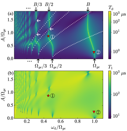
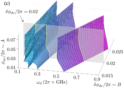
Figure 2: (a) Dynamical pure-dephasing time $T_{\phi}$ (color-coded) as a function of drive frequency $\omega_{\mathrm{d}}$ (horizontal axis) and drive amplitude $A$ (vertical axis). Results are calculated via Eq. (8) for flux $\delta\phi_{\mathrm{dc}}/2\pi=0.02$. The curves visible by their bright-yellow coloring are the dynamical sweet spots characterized by large $T_{\phi}$. In the weak ($A\ll\Omega_{ge}$) and strong drive limit ($A\gtrsim\Omega_{ge}$) these curves asymptotically line up with $\omega_{\mathrm{d}}=\Omega_{ge}/m$ and $\omega_{\mathrm{d}}=B/m$ (black arrows). The curves formed by the dynamical sweet spots are interrupted by cuts marked by white arrows. The overlaid white dotted curves depict the ac dynamical sweet spots corresponding to $\partial\epsilon_{01}/\partial\phi_{\mathrm{ac}}=0$. (b) Depolarization time $T_{1}$ calculated by Eq. (7). The majority of the obtained $T_{1}$ values are at the order of 500$\,\mu$s, except for point-like dropouts shown by the dark-blue coloring. The red star and triangle specify the dynamical sweet spots \raisebox{-.9pt} {1}⃝ and \raisebox{-.9pt} {2}⃝. The noise parameters used for the calculation are given in the caption of Table 1. (c) Sweet-spot manifolds embedded in the 3d parameter space, with axes corresponding to $\omega_{\mathrm{d}}$, $\delta\phi_{\mathrm{dc}}$ and $\phi_{\mathrm{ac}}$. The semi-transparent plane given by $\delta\phi_{\mathrm{dc}}/2\pi=0.02$, intersects the manifolds and thus yields the sweet-spot curves shown in (a) as cross sections (bright-yellow coloring).

This behavior of pure-dephasing times of the driven qubit can be explained and approximated analytically using Floquet theory. Away from dynamical sweet manifolds, $T_{\phi}$ is limited by contributions from the (regularized) pole of the $1/f$ spectrum, see the first term on the right-hand side of Eq. (8). Thus, $\gamma_{\phi}\propto|g_{0\phi}|$ which in turn can be shown to be proportional to $\partial\epsilon_{01}/\partial\phi_{\text{dc}}$ (see derivation in Appendix D), i.e., the dynamical flux-noise sensitivity given by the flux dispersion of the Floquet quasi-energy difference. We emphasize that this result is analogous to the more familiar case of the undriven qubit, where the pure-dephasing rate is proportional to the static flux dispersion $\partial\Omega_{ge}/\partial\phi_{\text{dc}}$, with quasi-energies replaced by eigenenergies.

Pure-dephasing times are maximal whenever

$$\frac{\partial\epsilon_{01}}{\partial\phi_{\mathrm{dc}}}\propto|g_{0\phi}|=0,$$ (9)

which generically occurs at avoided crossings in the extended quasi-energy spectrum [Fig. 1(b)]. The latter, analogous to the extended Brillouin zone in spatially periodic systems, consists of the extended set of quasi-energies $\epsilon_{j,n}=\epsilon_{j}+n\omega_{\mathrm{d}}$ ($n\in\mathbb{Z}$) [61, 62, 66]. This extended spectrum shows numerous avoided level crossings, and hence a multitude of regions of maximal $T_{\phi}$. These operation points are called dynamical sweet spots; see Refs. [19, 23, 24] for previous studies of this concept. Here, we specifically use this term to refer to the working points where the derivative of $\epsilon_{01}$ with respect to the noise parameter vanishes.

As shown in Fig. 2(a), these spots form a set of curves with maximal $T_{\phi}$ in the $A$-$\omega_{\text{d}}$ plane. Once we account for the additional perpendicular axis representing $B$, we find that each curve is the cross-section of a continuous surface of sweet spots, which we refer to as a sweet-spot manifold. The locations of sweet spots can be predicted in the limits of weak and strong drive, by treating either the drive $A\cos\omega_{\mathrm{d}}t\,\hat{\sigma}_{z}$ or the transverse qubit Hamiltonian $\Delta\,\hat{\sigma}_{x}/2$ perturbatively.

Weak-drive limit.— For $A\ll\Omega_{ge}$, the unperturbed quasi-energies are the static eigenenergies up to the addition of integer multiples of the drive frequency, $\epsilon_{\pm,n}=\pm\Omega_{ge}/2+n\omega_{\mathrm{d}}\,(n\in\mathbb{Z})$. Two levels exhibit a crossing, $\epsilon_{+,n}=\epsilon_{-,n^{\prime}}$, whenever the qubit frequency is an integer multiple of the drive frequency, $\Omega_{ge}=m\omega_{\mathrm{d}}$ where $m=n^{\prime}-n\in\mathbb{N}$. The perturbation lifts these degeneracies and generates avoided crossings. As a result, the sweet spots observed towards the bottom of Fig. 2(a) asymptotically take the form of vertical lines at drive frequencies set by $\omega_{\mathrm{d}}=\Omega_{ge}/m$. The width of maxima in $T_{\phi}(\omega_{\mathrm{d}})$ is significant for the issue of parameter deviations: the wider the maximum, the larger is the robustness of the coherence-time increase with respect to small detunings from the dynamical sweet spot. This width is proportional to the gap size of the avoided crossing and given by $\Delta_{m}\approx A^{m}|\sin\theta\cos^{m-1}\theta|/\omega_{\mathrm{d}}^{m-1}(m-1)!$ in the weak-drive limit, where $\theta=\tan^{-1}(\Delta/B)$ (see derivation in Appendix D). For decreasing drive strength $A$, the width narrows with $\sim A^{m}$ consistent with the behavior observed in Fig. 2(a).

Strong-drive limit.— For $A\gtrsim\Omega_{ge}$, the unperturbed quasi-energies are given by $\epsilon_{\pm,n}=\pm B/2+n\omega_{\mathrm{d}}$ ($n\in\mathbb{Z}$) and cross whenever $B=m\omega_{\mathrm{d}}$ ($m\in\mathbb{N}$) [62, 67, 64, 68]. The perturbation $\Delta\hat{\sigma}_{x}/2$ generically opens up gaps. The resulting sweet spots asymptotically line up with vertical intercepts $\omega_{\mathrm{d}}=B/m$, as shown in Fig. 2(a). The proportionality between the width of the maximal $T_{\phi}$ and the gap size also holds in this limit, with the latter given by $\Delta_{m}\approx\Delta|J_{m}(2A/\omega_{\mathrm{d}})|$ (see derivation in Appendix D). Whenever $\Delta_{m}=0$, i.e., $2A/\omega_{\mathrm{d}}$ is one of the roots of the Bessel function $J_{m}$, the width goes to zero and the sweet-spot curve is interrupted with a cut.

The dropouts of $T_{1}$ visible in Fig. 2(b) are similarly related to the vanishing gap size of the avoided crossings. If the gap opening of the avoided crossing, i.e., the quasi-energy difference of the qubit at the dynamical sweet spot becomes smaller, the terms $|g_{0\mp}|^{2}S(\pm\epsilon_{01})$ in Eq. (7) rapidly increase in magnitude as the regularized divergence of $S(\omega)$ is sampled. In other words, the low-frequency 1/$f$ noise significantly suppresses the dynamical $T_{1}$ whenever $\epsilon_{01}$ vanishes. Therefore, the low-$T_{1}$ features observed in Fig. 2(b) match the locations of strong narrowing of the maximal $T_{\phi}$ regions in Fig. 2(a) ($\Delta_{m}\to 0$), including the discussed cuts in the strong-drive limit, as well as the gradual narrowing in the weak-drive limit. In our example, the widths of $T_{\phi}$ peaks surrounding the sweet-spot manifolds are generally sufficiently wide and, hence, gap sizes sufficiently large, such that 1/$f$ flux noise does not limit the dynamical $T_{1}$.

Driving the qubit, as discussed above, efficiently decouples it from the low-frequency dc flux noise. Recent experimental evidence points to the relevance of additional noise in the ac drive amplitude [20, 21, 22, 19, 51]. While the magnitude and power spectrum of this noise are not well established, it is useful to note that there exist simultaneous sweet spots for the dc and ac flux amplitude, $\partial\epsilon_{01}/\partial\phi_{\mathrm{dc}}=\partial\epsilon_{01}/\partial\phi_{\mathrm{ac}}=0$. These doubly-sweet spots correspond to intersection points of the white dotted curves ($\partial\epsilon_{01}/\partial\phi_{\mathrm{ac}}=0$) and the underlying dc sweet-spot curves obtained for $\partial\epsilon_{01}/\partial\phi_{\mathrm{dc}}=0$ [see Fig. 2(a)] [69]. Depending on the magnitude of this ac noise, we expect such doubly-sweet spots to form the optimal working points.

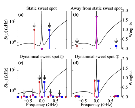
Figure 3: Noise spectra and filter weights centered at the corresponding filter frequencies. The panels refer to four different working points: (a) the static sweet spot, (b) static operation away from the sweet spot ($\phi_{\mathrm{dc}}/2\pi=0.52$), (c)-(d)dynamical sweet-spot operation at the working points \raisebox{-.9pt} {1}⃝ and \raisebox{-.9pt} {2}⃝. The symbols represent relaxation (blue squares), excitation (red diamonds), and pure dephasing (purple dots). The noise spectrum is plotted concurrently in (a)-(d). The positions of filter frequencies and the associated filter weights determine which components of the noise spectrum contribute significantly to the rates $\gamma_{\pm}$ and $\gamma_{\phi}$ [see Eqs. (7) and (8)]. (See the main text for the discussion of filter frequencies marked by arrows.)

IV.2 Interpretation of coherence times in terms of filter functions

We observe that, although the obtained dynamical $T_{1}$ and $T_{\phi}$ times in the sweet manifolds do not exceed the maximal values at the two static working points (see Table 1), they are well above the corresponding static minimal values. To understand this behavior, it is instructive to interpret the decoherence rates in terms of the sampling of the noise spectrum by the filter function [Eq. (5)]. For that purpose, Fig. 3 shows the noise spectrum $S(\omega)$ along with information characterizing the filter function $F_{\mu}(\omega)$ in terms of the relevant filter frequencies and weights. The noise spectrum (black curve) is peaked at $\omega=0$ due to the $1/f$ flux noise; away from that peak, dielectric loss dominates. For each filter frequency, the value of the corresponding filter weight is shown and marked by symbols distinguishing between depolarization and pure-dephasing channels. While there are only three filter frequencies in the static case, the dynamical case in principle produces an infinite number of filter frequencies $\bar{\omega}_{k\mu}$. The appearance of additional filter frequencies corresponds to the sampling of the noise spectral density at sideband frequencies, a point previously discussed for weakly driven systems in Refs. [48, 47, 49].

We first interpret the behavior of pure-dephasing times. The weight related to filter frequency $\bar{\omega}_{0\phi}$ is suppressed to zero for both static and dynamical sweet spots [see Fig. 3(a),(c),(d)], but is large for the working point away from sweet spot [see Fig. 2(b)]. This weight reflects the qubit’s sensitivity to $1/f$ flux noise. Therefore, the $T_{\phi}$ times at the sweet spots (both static and dynamical) are significantly longer than the one at the non-sweet spot. Compared with $T_{\phi}$ at the static sweet spot, the dynamical sweet spots exhibit somewhat lower values of $T_{\phi}$. This is related to the small but nonzero pure-dephasing weights at filter frequencies $\bar{\omega}_{k\phi}\neq 0$, absent for static sweet spots. Figure 3(c) illustrates this for the working point \raisebox{-.9pt} {1}⃝, where the relevant weights resulting in the dynamical $T_{\phi}\approx 1\,$ms are marked by single-headed arrows. (The same reasoning applies to the other working point \raisebox{-.9pt} {2}⃝.)

The behavior of depolarization times $T_{1}$ at and away from sweet spots is reversed relative to that of $T_{\phi}$. Specifically, $T_{1}$ is longest at the static non-sweet spot, where disjoint support of wave functions leads to the strongly suppressed weights marked by double-headed arrows in Fig. 3(b). By contrast, depolarization weights for sweet spots [both static and dynamical, Figs. 3(a),(c)] are not subject to this suppression and produce correspondingly lower $T_{1}$. [The $T_{1}$ trend obtained from the analysis of weight suppression is partially offset by the fact that $S(\omega)$ is filtered at different frequencies in the sweet-spot vs. non-sweet-spot case.] Next, the comparison shows that the static depolarization time at the sweet spot is smaller than the dynamical $T_{1}$. The reason for this can be traced to the difference in filter frequencies and corresponding magnitudes of the noise power spectrum, see Fig. 3(a) vs. (c). In the static case, the filter frequencies for depolarization are $\pm\Omega_{ge}$, and $S(\pm\Omega_{ge})$ is relatively large compared to the dynamical case in 3(c) where the dominant contributions arise from $S(\bar{\omega}_{0\pm})$. Indeed, these latter contributions closely match the minima of the noise power spectrum – a situation which can be established simply by tuning the drive parameters.

Inspection of Tab. 1 reveals a trend of $T_{1}$ and $T_{\phi}$ being anti-correlated: larger $T_{1}$ tend to coincide with with smaller $T_{\phi}$ and vice versa. This trend originates from the conservation of the cumulative filter weight,

$$(W_{+}+W_{-})+W_{\phi}=2,$$ (10)

where $W_{\pm}=\sum_{k}|g_{k\pm}|^{2}$ governs depolarization and $W_{\phi}=\sum_{k}2|g_{k\phi}|^{2}$ pure dephasing. (A proof of this conservation law is given in Appendix C.) Increases in depolarization weights thus go along with decreases in the pure-dephasing weight, creating a tendency for trade-off between depolarization and dephasing which is exact only in the special case of white noise. This conservation rule is analogous to the sum rule that emerges in the context of dynamical decoupling [39, 18]. It is crucial that the conservation rule applies to filter weights rather than the rates. This enables one to manipulate the distribution of weights and filter frequencies to our advantage, putting the largest weights at or near minima in the noise spectrum.

For simplicity, our discussion has been based exclusively on a two-level approximation of the fluxonium qubit. In general, the presence of higher qubit levels can induce leakage to states outside the computational subspace. This concern is less significant for qubits with relatively large anharmonicity like the fluxonium circuit considered here. Through numerical calculations including higher levels we have confirmed that this leads to quantitative changes of the dynamical decoherence rates above, but does not affect the results reported above qualitatively.

V Gates and Readout of a single Floquet qubit

The above results suggest that use of the driven Floquet states as computational qubit states can be advantageous due to the long coherence times reached at the dynamical sweet spots. We refer to this dynamically protected qubit as the Floquet qubit, which belongs to the broader class of dressed-state qubits. A host of previous work has studied gate operations on such dynamically encoded qubits [70, 25, 26, 71, 72]. Here, we specifically discuss how to maintain dynamical-sweet-spot operation while performing gates in order to maximize protection from $1/f$ noise. In the following, we show that Floquet qubits can easily be integrated into gate and readout protocols necessary for quantum-information processing.

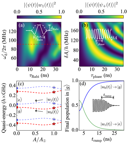
Figure 4: Concurrent gates for the Floquet qubit and adiabatic mapping protocol for readout. (a) Adding a secondary pulse (inset) to the Floquet drive induces Rabi oscillations, which are sufficient for implementing $X$ gate operations. The plot shows the final population in Floquet eigenstate $|w_{1}(t)\rangle$ as a function of pulse duration $\tau_{\mathrm{Rabi}}$ and carrier frequency $\omega_{\mathrm{d}}^{\prime}$, for the initial state $|w_{0}(t)\rangle$. Full Rabi oscillations are observed when the secondary drive frequency matches the quasi-energy difference $\epsilon_{01}$ (dashed line) (b) Phase gates can be realized by a temporary increase in the Floquet drive strength (inset). The change in drive strength modulates the quasi-energy and thus enables phase gates such as $S\,(\pi/2)$ and $T\,(\pi/4)$. The plot shows the final population in $|\psi_{+}(t)\rangle$, as a function of the pulse duration $\tau_{\mathrm{phase}}$ and the drive amplitude variation $\delta A$, with the qubit initialized in $|\psi_{-}(t)\rangle$ (see main text for definition for $|\psi_{\pm}(t)\rangle$). (c) shows the quasi-energy spectrum as a function of $A$ (from 0 to $A_{\scriptsize{\raisebox{0.5pt}{\raisebox{-.9pt} {1}⃝}{}}}$), with Floquet drive frequency fixed at $\omega_{\mathrm{d}\scriptsize{\raisebox{0.5pt}{\raisebox{-.9pt} {1}⃝}{}}}$. ($A_{\scriptsize{\raisebox{0.5pt}{\raisebox{-.9pt} {1}⃝}{}}}$ and $\omega_{\mathrm{d}\scriptsize{\raisebox{0.5pt}{\raisebox{-.9pt} {1}⃝}{}}}$ are the drive parameters at working point \raisebox{-.9pt} {1}⃝.) Red and blue star symbols mark the two Floquet states at point \raisebox{-.9pt} {1}⃝, whereas dots of the same color represent the states $|g\rangle$ and $|e\rangle$ of the undriven fluxonium. An adiabatic mapping from Floquet states to static qubit eigenstates can by realized with a sufficiently slow switch-off of the drive from $A_{\scriptsize\raisebox{0.5pt}{\raisebox{-.9pt} {1}⃝}{}}$ to 0, given the nonzero gap between the quasi-energies. (d) Simulation of the adiabatic mapping achieved by continuously switching off the drive (ramp-down in inset). The final population in $|g\rangle$ is plotted as a function of the ramp time $t_{\mathrm{ramp}}$, with the qubit initiated in $|w_{0}(t)\rangle$ (blue) or $|w_{1}(t)\rangle$ (green). The results confirm the feasibility of an adiabatic mapping with high fidelity, thus enabling readout of the Floquet states.

V.1 Gate operations

We show that we can realize direct single-qubit gates on the Floquet qubit. For example, $X$ and $\sqrt{X}$ gates can be realized by inducing Rabi oscillations among Floquet eigenstates. This is accomplished by applying an additional pulse with carrier frequency $\omega_{\mathrm{d}}^{\prime}\approx\epsilon_{01}$, duration $\tau_{\mathrm{Rabi}}$, and maximal amplitude $d_{\mathrm{Rabi}}$, see inset of Fig. 4(a). We verify the presence of Rabi oscillations numerically by simulating the time evolution for the working point \raisebox{-.9pt} {1}⃝. For a fixed initial state $|w_{0}(t)\rangle$, the final population of $|w_{1}(t)\rangle$ shows oscillatory behavior as a function of $\tau_{\mathrm{Rabi}}$ and $\omega^{\prime}_{\mathrm{d}}$, see Fig. 4(a). Full Rabi cycles only occur when $\omega^{\prime}_{\mathrm{d}}$ matches $\epsilon_{01}$. Computation of the gate fidelities for the examples of $X$ and $\sqrt{X}$ gates yields a value of $99.99\%$ in both cases.

Single-qubit phase gates can be implemented by modulating the quasi-energy difference $\epsilon_{01}$ through a temporary increase $\delta A$ of the drive amplitude [see inset of Fig. 4(b)]. This modifies the dynamical phase acquired over the gate duration $\tau_{\text{phase}}$, enabling $S$ and $T$ gates, for example. For numerical verification, we initialize the qubit in one of the Floquet superposition states $|\psi_{\pm}(t)\rangle=[|w_{0}(t)\rangle\pm|w_{1}(t)\rangle\mathrm{e}^{-i\epsilon_{01}t}]/\sqrt{2}$ (equator of the Bloch sphere) and monitor the population in the orthogonal state as a function of $\tau_{\text{phase}}$ and $\delta A$. The observed oscillations [Fig. 4(b)] in this population indicates that the computational states accumulate a relative phase as expected. The computed fidelity for $S$ ($\pi/2$) and $T$ ($\pi/4$) gates realized both exceed $99.99\%$.

V.2 Readout

Floquet states can be adiabatically mapped [73, 63] to the eigenstates of the driven qubit by slowly ramping down the flux modulation, provided that gaps in the quasi-energy spectrum are sufficiently large. For \raisebox{-.9pt} {1}⃝, Fig. 4(c) shows that quasi-energy gaps do not close as $A$ is decreased to 0, thus enabling the adiabatic state transfer. We verify this mapping numerically by simulating the closed-system evolution with either of the driven Floquet qubit eigenstates $|w_{0(1)}(t)\rangle$ as the initial state and a smooth ramp-down of duration $t_{\text{ramp}}$. Fig. 4(d) shows the calculated population in the undriven qubit eigenstates $|g(e)\rangle$ as a function of time. The resulting state-transfer fidelity is high for ramp times of the order of tens of ns, ($99.6\%$ for $t_{\mathrm{ramp}}=30\,$ns). Conventional dispersive readout techniques, applicable to fluxonium qubits [13, 12, 14, 7, 8], can then be employed subsequently in order to infer the original dynamical state.

In future work, it may be interesting to explore alternative readout protocols similar to the one presented in [8]. In an extension of that scheme, a higher fluxonium level that produces a large dispersive shift on the readout resonator would be excited conditionally, based on the occupied computational Floquet state.

VI Floquet two-qubit gates

The fact that dynamical sweet spots form entire manifolds in the control-parameter space provides sufficient flexibility to perform two-qubit gates among Floquet qubits without ever giving up the dynamical protection. Thanks to the one-to-one relation between quasi-energies and Floquet states on one hand, and ordinary eigenenergies and eigenstates on the other hand, it is possible to transfer existing protocols for two-qubit gates to the case of Floquet qubits. In the following, we present a protocol for implementing a $\sqrt{i\textrm{SWAP}}$ gate between two Floquet qubits, again based on flux-modulated fluxonium qubits. Related protocols for implementing two-qubit gates with dynamical protection have been discussed for slightly different systems involving either near-adiabatic parametric modulation of the qubit frequency [19, 20, 21, 23] or requiring a tunable coupler between qubits [74, 75]. The two-qubit gate proposed here is designed for the protected Floquet regime discussed above. It is compatible with direct driving of the qubit and circumvents the need for tunable coupling, thus providing a relatively simple scheme for future experimental realization.

VI.1 Analytical description

A simple method of implementing $\sqrt{i\textrm{SWAP}}$ gates, for example among two transmon qubits, consists of bringing the pair of weakly coupled qubits into resonance for a certain gate duration. For two Floquet qubits, we show that $\sqrt{i\textrm{SWAP}}$ gates can realized in a similar manner by tuning the quasi-energy differences into and out of resonance. An important advantage of the Floquet two-qubit gate is the ability to keep both qubits within the dynamical sweet manifolds for the complete duration of the gate, thus reducing the error due to the qubits’ coupling to 1/$f$ noise.

We establish this Floquet-gate protocol for a composite system of two coupled fluxonium qubits, each of which is flux-modulated, described by

$$\hat{H}_{\mathrm{LR}}(t)=\hat{H}_{\mathrm{L}}(t)+\hat{H}_{\mathrm{R}}(t)+\hat{H}_{\mathrm{int}}.$$ (11)

Here, $\hat{H}_{\mathrm{L}}(t)$ and $\hat{H}_{\mathrm{R}}(t)$ denote the Hamiltonians of the two periodically driven fluxonium qubits, and $\hat{H}_{\mathrm{int}}$ is the time-independent coupling between them. The flux-modulation frequencies associated with the two qubits are given by $\omega^{\mathrm{L}}_{\mathrm{d}}$ and $\omega^{\mathrm{R}}_{\mathrm{d}}$, respectively. As appropriate for a fluxonium with large anharmonicity, we may simplify the description by truncating the Hilbert space to a two-level subspace. We propose to induce the necessary qubit-qubit interaction $H_{\mathrm{int}}$ via a mutual inductance between the two fluxonium loops. In this case, the coupling term takes the form $\hat{H}_{\mathrm{int}}=J\hat{\sigma}^{\mathrm{L}}_{z}\hat{\sigma}^{\mathrm{R}}_{z}$, with $J$ denoting the coupling strength. For later convenience, we introduce the abbreviation $\hat{H}_{0}(t)=\hat{H}_{\mathrm{L}}(t)+\hat{H}_{\mathrm{R}}(t)$ for the bare qubit Hamiltonian.

When the two Floquet qubits are in resonance, i.e., their quasi-energies are degenerate, then the static coupling induces excitation swapping between the Floquet states (rather than between bare qubit eigenstates). To describe this process, we move to the interaction picture using the time-dependent unitary $\hat{U}_{0}(t)=\,\mathcal{T}\exp[-i\int_{0}^{t}\hat{H}_{0}(t^{\prime})dt^{\prime}]=\hat{U}^{\mathrm{L}}_{\mathrm{q}}(t)\otimes\hat{U}^{\mathrm{R}}_{\mathrm{q}}(t)$. Here, $\hat{U}^{\mathrm{L(R)}}_{\mathrm{q}}(t)=\sum_{j=0,1}|w^{\mathrm{L(R)}}_{j}(t)\rangle\langle w^{\mathrm{L(R)}}_{j}(0)|\exp[-i\epsilon^{\mathrm{L(R)}}_{j}t]$, and $|w_{j}^{\mathrm{L(R)}}(t)\rangle$ and $\epsilon^{\mathrm{L(R)}}_{j}$ denote the $j$-th Floquet state and corresponding quasi-energy of the left (right) qubit. In this interaction picture, the Hamiltonian is given by

$$\tilde{H}_{\mathrm{LR}}(t)= J\,\hat{U}^{\dagger}_{0}(t)\hat{\sigma}^{\mathrm{L}}_{z}\hat{\sigma}^{\mathrm{R}}_{z}\hat{U}_{0}(t)$$

$$= J\!\sum_{k,k^{\prime}\in\mathbb{Z}}\sum_{\mu,\mu^{\prime}=\pm,\phi}\!g^{\mathrm{L}}_{k\mu}g^{\mathrm{R}}_{k^{\prime}\mu^{\prime}}\hat{c}^{\mathrm{L}}_{\mu}\hat{c}^{\mathrm{R}}_{\mu^{\prime}}$$

$$\times\exp\!\left[-i(\bar{\omega}^{\mathrm{L}}_{k\mu}\!+\!\bar{\omega}^{\mathrm{R}}_{k^{\prime}\mu^{\prime}})t\right]\!,$$ (12)

where $\bar{\omega}^{\mathrm{L(R)}}_{k\mu}$ and $g^{\mathrm{L(R)}}_{k\mu}$ are the filter frequencies and the Fourier coefficients of the $\hat{\sigma}^{\mathrm{L(R)}}_{z}$’s matrix elements in the Floquet basis, associated with the left (right) qubit, respectively. The operators $\hat{c}^{\mathrm{L(R)}}_{\mu}$ denote the Pauli matrices defined in the Floquet basis (see Appendix B for details).

Following the conventional strategy, we perform a $\sqrt{i\textrm{SWAP}}$ gate by bringing the Floquet qubits into resonance ($\epsilon^{\mathrm{L}}_{01}=\epsilon^{\mathrm{R}}_{01}$) through an suitable change of the drive parameters. After rotating-wave approximation, the effective Hamiltonian at the degeneracy point reduces to

$$\tilde{H}^{\prime}=J\,g^{\mathrm{L}}_{0+}g^{\mathrm{R}}_{0-}\hat{c}^{\mathrm{L}}_{+}\hat{c}^{\mathrm{R}}_{-}+\mathrm{h.c.},$$ (13)

which is the flip-flop interaction necessary for the $\sqrt{i\textrm{SWAP}}$ gate. We note that the term proportional to $g^{\mathrm{L}}_{0\phi}g^{\mathrm{R}}_{0\phi}\hat{c}^{\mathrm{L}}_{\phi}\hat{c}^{\mathrm{R}}_{\phi}$ corresponds to an unwanted $Z\!Z$ interaction between Floquet qubits. This term exactly vanishes as soon as at least one of the qubits is at a dynamical sweet spot where $g_{0\phi}^{\mathrm{L,R}}=0$ [Eq. (9)].

Based on the full interaction Hamiltonian (VI.1), we next verify numerically that this simple strategy indeed yields high-fidelity two-qubit gates.

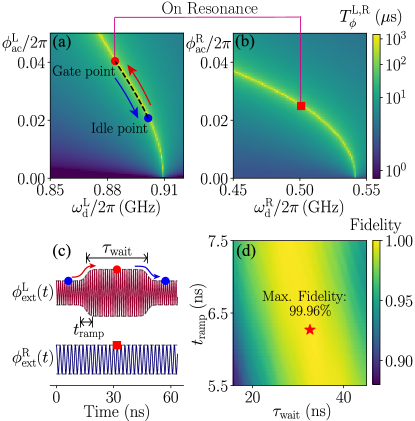
Figure 5: Simulation of a Floquet-$\sqrt{i\textrm{SWAP}}$ gate for two inductively coupled fluxonium qubits. (a) and (b) show the dynamical sweet manifolds corresponding to the two driven fluxonium qubits, at given dc flux biases. The red and blue dots in (a) indicate the gate and idle points for the left fluxonium, which is tuned along the path marked by the black-dashed curve. The red square in (b) represents the operating point for the right fluxonium qubit. (c) shows the drive pulses realizing this gate operation with $\tau_{\mathrm{wait}}$ and $t_{\mathrm{ramp}}$ denoting gate duration and ramp time, respectively. (d) depicts the calculated gate fidelity as a function of ramp time and gate duration, where the red star marks the position of maximal gate fidelity. (Parameters are as follows: left fluxonium – $E_{\mathrm{C}}^{\mathrm{L}}/h=1.2\,$GHz, $E_{\mathrm{J}}^{\mathrm{L}}/h=6.0\,$GHz; right fluxonium – $E_{\mathrm{L}}^{\mathrm{L}}/h=0.95\,$ GHz, while $E_{\mathrm{C}}^{\mathrm{R}}/h=1.0\,$GHz, $E_{\mathrm{J}}^{\mathrm{R}}/h=4.1\,$GHz, and $E_{\mathrm{L}}^{\mathrm{R}}/h=0.7\,$ GHz. The interaction strength is set by $J/h=4.8\,$MHz. The dc fluxes are fixed to $\phi^{\mathrm{L(R)}}_{\mathrm{dc}}/2\pi=0.529(0.520)$, and noise parameters are the same as in Table 1.)

VI.2 Numerical simulation

To construct our $\sqrt{i\textrm{SWAP}}$ gate, we first identify appropriate drive parameters for sweet-spot operation and for bringing the qubits into and out of resonance. Fig. 5(a) and (b) show the relevant sweet-spot manifolds for the two fluxonium qubits. Within these manifolds, the quasi-energy difference $\epsilon^{\mathrm{L,R}}_{01}$ varies continuously, making it possible to establish degeneracy of the two Floquet qubit quasi-energies, $\epsilon^{\mathrm{L}}_{01}=\epsilon^{\mathrm{R}}_{01}$. In the example we selected, the right qubit is maintained at a fixed dynamical sweet spot [Fig. 5(b), red square] while the left qubit can be tuned within its sweet-spot manifold from an idle point (blue dot) into resonance at the gate point (red dot) and back [Fig. 5(a)].

The detailed pulse shapes of the drives enacting the gate are shown in Fig. 5(c). For the left fluxonium qubit, amplitude and frequency of the flux modulation are adjusted in a way to smoothly tune the qubit from its idle point to the gate point (within the ramp time $t_{\mathrm{ramp}}$). Pulse shaping allows one to choose a path (black-dashed curve) that keeps the Floquet qubit within the sweet manifold [Fig. 5(a)]. After leaving the qubit at the gate point for a suitable waiting time $\tau_{\mathrm{wait}}$, the drive parameters are tuned back to the idle point. We calculate the $\sqrt{i\textrm{SWAP}}$-gate fidelity by an open-system simulation of this composite system (again taking into account of $1/f$ flux noise and dielectric loss). The results in Fig. 5(d) show a broad region of gate parameters $\tau_{\mathrm{wait}}$ and $t_{\mathrm{ramp}}$ with high gate fidelities up to $99.96\%$. (The discussion of the effect of stray two-qubit interactions at the idle point is beyond the scope of this paper, but see Refs. [76, 75, 77, 78, 79] for mitigation strategies.)

VII Conclusions

Operation of superconducting qubits at static sweet spots is a well-established means to reducing 1/$f$ noise sensitivity. However, one limitation is the abrupt symmetry-induced change in the nature of wavefunctions at the sweet spot, which can negatively impact depolarization times at the sweet spot. We have presented a protocol for engineering dynamical sweet spots which partially overcome this limitation. In contrast to static sweet-spot operation, the Floquet scheme can yield long dynamical $T_{\phi}$ and $T_{1}$ simultaneously. The possibility to directly perform both single- and two-qubit gate operations as well as readout on Floquet qubits makes them promising for both quantum information storage and processing. A companion experimental work has implemented this proposed protocol using a flux-modulated fluxonium qubit [51], and a 40-fold improvement in dephasing time due to dynamical sweet-spot operation is reported.

Although the example we have demonstrated only makes use of the simplest single-tone drives, it is possible that non-sinusoidal or multichromatic drives could further expand the sweet-spot manifolds and yield even higher qubit coherence times. Future work may explore building networks of larger numbers of Floquet qubits, which could be particularly beneficial for quantum information processing thanks to enhanced dynamical coherence times and tunability.

Appendix A Effective model for fluxonium, and coupling to noise sources

The Hamiltonian describing a flux-modulated fluxonium is given by [80]

$$H_{\mathrm{q,full}}(t)=4E_{\mathrm{C}}\hat{n}^{2}+\frac{1}{2}E_{\mathrm{L}}[\hat{\varphi}+\phi_{\mathrm{ext}}(t)]^{2}-E_{\mathrm{J}}\cos\hat{\varphi},$$ (14)

where $E_{\mathrm{C}}$, $E_{\mathrm{L}}$ and $E_{\mathrm{J}}$ represent the capacitive, inductive and Josephson energies of the fluxonium qubit, and $\phi_{\mathrm{ext}}(t)=\phi_{\mathrm{dc}}+\phi_{\mathrm{ac}}\cos(\omega_{\mathrm{d}}t)$. We use $\hat{\varphi}$ and $\hat{n}$ to denote the flux and conjugate charge operator of the qubit, respectively.

The static eigenenergies $\Omega_{l}$ and corresponding eigenstates $|l\rangle$ ($l=g,e,f,\cdots$) are obtained by diagonalizing $H_{\mathrm{q,full}}$, and depend on the dc flux component $\phi_{\text{dc}}$. We will refer to the specific solutions at the static sweet spot $\phi_{\mathrm{dc}}=\pi$ by $\widetilde{\Omega}_{l}$ and $\big{|}\tilde{l}\big{\rangle}$. These eigenstates, expressed in the phase basis, have alternating parities (for example, $|\tilde{g}\rangle$ and $|\tilde{e}\rangle$ have even and odd parities respectively).

To avoid leakage into higher fluxonium states under flux modulation, we choose fluxonium parameters resulting in a large anharmonicity at half-integer flux, $\widetilde{\Omega}_{f}-\widetilde{\Omega}_{e}\gg\widetilde{\Omega}_{e}-\widetilde{\Omega}_{g}$. If we limit the external flux $\phi_{\mathrm{ext}}(t)$ to values in the vicinity of $\phi_{\mathrm{dc}}=\pi$, and avoid resonance with the $e-f$ transition, $\omega_{\mathrm{d}}\ll\widetilde{\Omega}_{f}-\widetilde{\Omega}_{e}$, then Eq. (14) can be approximated by the effective two-level Hamiltonian (1). In that Hamiltonian, $\Delta=\widetilde{\Omega}_{e}-\widetilde{\Omega}_{g}$, $A=E_{\mathrm{L}}\phi_{\mathrm{ac}}\tilde{\varphi}_{ge}$, $B=2E_{\mathrm{L}}(\phi_{\mathrm{dc}}-\pi)\tilde{\varphi}_{ge}$; here, $\tilde{\varphi}_{ge}=|\langle\tilde{g}|\hat{\varphi}|\tilde{e}\rangle|$. Different from the usual convention, we define the Pauli matrices as

$$\sigma_{x}=|\tilde{e}\rangle\langle\tilde{e}|-|\tilde{g}\rangle\langle\tilde{g}|,\quad\sigma_{z}=|\tilde{g}\rangle\langle\tilde{e}|+|\tilde{e}\rangle\langle\tilde{g}|,$$ (15)

which is a common choice in the context of flux qubits [62, 63].

Given this effective model, it is important to revisit the question of how the fluxonium qubit couples to the limiting environment degrees of freedom. In Section II, it is posited that the noise sources of interest couple to the qubit through its $\sigma_{z}$ operator which can be motivated as follows. The fluxonium’s interaction with the $1/f$ flux noise source can be modeled as mutual inductance between the fluxonium’s inductor and the bath, hence the coupling to the noise is via the qubit operator $\hat{\varphi}$. Experimental results are further consistent with dielectric noise coupling to the qubit’s phase operator [7, 13, 14, 8, 16]. Note that operator $\hat{\varphi}$ only couples states with different parities. Therefore, based on Eq. (15), it is projected to $\sigma_{z}$ in the two-level subspace, which results in the $H_{\mathrm{int}}$ used in our model.

Appendix B Floquet master equation

This appendix sketches the derivation of the Floquet master equation [60, 61, 64] which we use in the subsequent appendix to calculate the dynamical decoherence rates. The full Hamiltonian is given by $H(t)=H_{\mathrm{q}}(t)+H_{\mathrm{B}}+H_{\mathrm{int}}$ with time-periodic qubit Hamiltonian, and time-independent bath and interaction Hamiltonian. The latter is taken to be of the form $H_{\mathrm{int}}=\hat{\sigma}\hat{\eta}$, where $\hat{\sigma}$ and $\hat{\eta}$ are qubit and bath operators, respectively.

We start from the Redfield equation of the driven qubit

$$\frac{\mathrm{d}\tilde{\rho}_{\mathrm{q}}(t)}{\mathrm{d}t}\!=\!-\!\int_{0}^{t}d\tau\text{Tr}_{\mathrm{B}}\!\left[\tilde{H}_{\mathrm{int}}(t),\left[\tilde{H}_{\mathrm{int}}(t-\tau),\tilde{\rho}_{\mathrm{q}}(t)\!\otimes\!\tilde{\rho}_{\mathrm{B}}\right]\right]\!,$$ (16)

which describes the evolution of the qubit density matrix $\tilde{\rho}_{\mathrm{q}}$ (in the interaction picture). Here, $\mathrm{Tr}_{\mathrm{B}}$ denotes a partial trace on the bath degrees of freedom, and $\tilde{\rho}_{\mathrm{B}}$ is the density matrix of the bath in the interaction picture, which is assumed to stay in thermal equilibrium. The term $\tilde{H}_{\mathrm{int}}(t)=U_{0}^{\dagger}(t)H_{\mathrm{int}}U_{0}(t)$ is the qubit-bath coupling expressed in the interaction picture, where $U_{0}(t)=U_{\mathrm{q}}(t)U_{\mathrm{B}}(t)$, $U_{\mathrm{q}}(t)=\sum_{j=0,1}|w_{j}(t)\rangle\langle w_{j}(0)|\exp(-i\epsilon_{j}t)$, and $U_{\mathrm{B}}(t)=\exp(-iH_{\mathrm{B}}t)$. The interaction term can be further expressed as $\tilde{H}_{\mathrm{int}}(t)=\tilde{\sigma}(t)\tilde{\eta}(t)$, where $\tilde{\sigma}(t)=U^{\dagger}_{\mathrm{q}}(t)\hat{\sigma}U_{\mathrm{q}}(t)$ and $\tilde{\eta}(t)=U^{\dagger}_{\mathrm{B}}(t)\hat{\eta}U_{\mathrm{B}}(t)$.

Eq. (16) is an integro-differential equation, and not convenient for reading off decoherence rates. To derive expressions for $\gamma_{\mu}$ ($\mu=\pm,\phi$), we first simplify this equation by employing the rotating-wave approximation. In order to identify the fast-rotating terms, we decompose $\tilde{\sigma}(t)$ into different frequency components,

$$\tilde{\sigma}(t)=\,\sum_{k\in\mathbb{Z},\mu=\pm,\phi}g_{k\mu}\hat{c}_{\mu}(0)\exp(-i\bar{\omega}_{k\mu}t).$$ (17)

Here, we define the Floquet counterparts of the Pauli matrices by

$$\hat{c}_{+}(t)= \,|w_{1}(t)\rangle\langle w_{0}(t)|,$$

$$\hat{c}_{-}(t)= \,|w_{0}(t)\rangle\langle w_{1}(t)|,$$

$$\hat{c}_{\phi}(t)= \,|w_{1}(t)\rangle\langle w_{1}(t)|-|w_{0}(t)\rangle\langle w_{0}(t)|.$$ (18)

The frequencies $\bar{\omega}_{k,\mu}$ appearing in Eq. (17) are the filter frequencies defined in the Section III, namely $\bar{\omega}_{k\pm}=\mp\epsilon_{01}+k\omega_{\mathrm{d}}$ and $\bar{\omega}_{k\phi}=k\omega_{\mathrm{d}}$. Furthermore, the Fourier-transformed coupling matrix elements are given by

$$g_{k,\pm}= \frac{\omega_{\mathrm{d}}}{2\pi}\int_{0}^{2\pi/\omega_{\mathrm{d}}}\mathrm{d}t\,e^{ik\omega_{\mathrm{d}}t}\,\operatorname{Tr}_{\mathrm{q}}\left[\hat{\sigma}\hat{c}_{\mp}(t)\right],$$

$$g_{k,\phi}= \frac{\omega_{\mathrm{d}}}{4\pi}\int_{0}^{2\pi/\omega_{\mathrm{d}}}\mathrm{d}t\,e^{ik\omega_{\mathrm{d}}t}\,\operatorname{Tr}_{\mathrm{q}}\left[\hat{\sigma}\hat{c}_{\phi}(t)\right],$$ (19)

where $\operatorname{Tr}_{\mathrm{q}}$ is the partial trace over the qubit degrees of freedom.

The qubit interaction operator $\tilde{\sigma}(t)$, expanded in this way, is substituted into Eq. (16) resulting in a sum terms each involving the coefficient $\exp[-i(\bar{\omega}_{k^{\prime}\mu^{\prime}}-\bar{\omega}_{k\mu})t]$. Under certain conditions, every term with $\bar{\omega}_{k^{\prime}\mu^{\prime}}-\bar{\omega}_{k\mu}\neq 0$ can be treated as fast-rotating and be neglected. This strategy is appropriate if both the minimal quasi-energy difference and the drive frequency $\omega_{\mathrm{d}}$ are much larger than the inverse of the relevant time scale, i.e., the coherence time. With this Eq. (16) is cast into the simplified form

$$\frac{\mathrm{d}\tilde{\rho}_{\mathrm{q}}(t)}{\mathrm{d}t}=\sum_{\mu=\pm,\phi}\zeta_{\mu}\left[\int_{-\infty}^{\infty}{\mathrm{d}\omega}F_{\mu}(\omega,t)S(\omega)\right]\mathbb{D}[\hat{c}_{\mu}]\tilde{\rho}_{\mathrm{q}}(t),$$ (20)

where

$$F_{\mu}(\omega,t)=\zeta^{-1}_{\mu}\sum_{k}\pi^{-1}t\,\textrm{sinc}[(\omega-\bar{\omega}_{k\mu})t]|g_{k\mu}|^{2}$$ (21)

denotes the filter functions from Section III, $\mathbb{D}[L]\tilde{\rho}_{\mathrm{q}}=L\tilde{\rho}_{\mathrm{q}}L^{\dagger}-(L^{\dagger}L\tilde{\rho}_{\mathrm{q}}+\tilde{\rho}_{\mathrm{q}}L^{\dagger}L)/2$ is the usual damping superoperator, and $S(\omega)=\int_{-\infty}^{\infty}\mathrm{d}t\,e^{i\omega t}\operatorname{Tr}_{\mathrm{B}}[\tilde{\eta}(t)\tilde{\eta}(0)\tilde{\rho}_{\mathrm{B}}]$ is the noise spectrum. We have further introduced the abbreviations $\zeta_{\pm}\equiv 1$ and $\zeta_{\phi}\equiv 1/2$, and used $\hat{c}_{\mu}(0)\to\hat{c}_{\mu}$. [We note that terms contributing to the Lamb shift have been omitted in Eq. (20).]

The simplified Redfield equation (20) is reminiscent of the Lindblad form, and includes three distinct terms $\mu=\pm$ and $\mu=\phi$ that describe relaxation, excitation and pure dephasing of the Floquet qubit. However, in place of fixed rates associated with the individual jump terms, Eq. (20) still involves time-dependent rate coefficients given by

$$K_{\mu}(t)=\int_{-\infty}^{\infty}\mathrm{d}\omega F_{\mu}(\omega,t)S(\omega).$$ (22)

We discuss in the subsequent appendix how to evaluate these rate coefficients for concrete choices of the noise spectrum $S(\omega)$.

Appendix C Evaluation of decoherence rates

This appendix discusses the evaluation of the decoherence rate coefficients associated with the simplified Redfield equation (20), focusing on the specific noise spectrum $S(\omega)$ adopted in the main text. To simplify the integral $K_{\mu}(t)$, we first inspect the structure of the filter functions $F_{\mu}(\omega,t)$ defined in Eq. (21). These functions are peaked at the filter frequencies $\bar{\omega}_{k,\mu}$, with the peak width given by $2\pi t^{-1}$. We distinguish two separate scenarios: (1) the case of noise spectra that can be approximated as constant within each peak width, and (2) the case of noise spectra, such as $1/f$ spectra, where this approximation does not hold for all peaks.

Case (1).—If the spectrum $S(\omega)$ is sufficiently flat within each peak-width frequency range, we can approximate $(t/\pi)\,\mathrm{sinc}(\omega t)\approx\delta(\omega)$ in Eq. (21), and arrive at the Markovian Floquet master equation

$$\frac{\mathrm{d}\tilde{\rho}_{\mathrm{q}}(t)}{\mathrm{d}t}=\sum_{k\in\mathbb{Z},\mu=\pm,\phi}|g_{k\mu}|^{2}S(\bar{\omega}_{k\mu})\mathbb{D}[\hat{c}_{\mu}]\tilde{\rho}_{\mathrm{q}}(t).$$ (23)

This form allows one to directly read off the resulting rates which are given by $\gamma_{\pm}=\sum_{k}|g_{k\mu}|^{2}S(\bar{\omega}_{k\pm})$ and $\gamma_{\phi}=\sum_{k}2|g_{k\phi}|^{2}S(\bar{\omega}_{k\phi})$.

Case (2).—On the other hand, the noise spectrum $S(\omega)$ at depolarization filter frequencies $\bar{\omega}_{k\pm}$ is considered flat, therefore the resulting expressions of $\gamma_{\pm}$ is the same as shown in Case (1). Finally, we arrive at the results shown in Eqs. (7) and (8) in the main text.

Whenever the noise spectrum varies significantly across one filter-function peak width, the above approximation fails. This is, in particular, the case for $1/f$ noise near $\omega=0$ where $S(\omega)$ is purely dominated by the contribution $S_{\mathrm{f}}(\omega)=\mathcal{A}_{f}^{2}|\omega/2\pi|^{-1}$. For filter frequencies away from $\omega=0$, we continue treating $S(\omega)$ as sufficiently flat. Zero and nonzero filter frequencies hence play distinct roles. For depolarization, relevant filter frequencies $\bar{\omega}_{k\pm}$ are non-zero and the discussion of Case (1) carries over, yielding Eq. (7) for the depolarization rates.

The appearance of a zero filter frequency for dephasing motivates us to separate the integral $K_{\phi}(t)$ [Eq. (22)] into a low-frequency and a high-frequency part. We focus on the low-frequency part first, which is given by

$$I(t)=2|g_{0\phi}|^{2}\int_{-\pi/t}^{\pi/t}\mathrm{d}\omega\,\frac{t}{\pi}\,\mathrm{sinc}(\omega t)S_{\mathrm{f}}(\omega),$$ (24)

where the integration range is set by the peak width $2\pi/t$. To regularize the logarithmic divergence of this integral, we employ infrared cutoffs $\pm\omega_{\mathrm{ir}}$ [5, 17, 20, 56]. The cutoff is of the order of $1\,$Hz [17], much smaller than the inverse of the measurement time. In this case, the integral can be approximated by

$$I(t)\approx 8\mathcal{A}^{2}_{\mathrm{f}}t|\ln\omega_{\mathrm{ir}}t||g_{0\phi}|^{2}.$$ (25)

For the integral over the remaining high-frequency range, the $\delta$-function approximation we made in Case (1) is again valid. After combining the low and high-frequency contributions, the approximated $K_{\phi}(t)$ is a time-dependent function, given by

$$K_{\phi}(t)\approx I(t)+2\sum_{k\neq 0}|g_{k\phi}|^{2}S(\bar{\omega}_{k\phi}).$$ (26)

According to this, $K_{\phi}(t)$ is reminiscent of a time-dependent rate for pure dephasing that grows linearly in time (up to logarithmic corrections). Consequently, the off-diagonal elements of the density matrix do not follow an exponential decay. Instead, the decay is given by

$$\tilde{\rho}_{\mathrm{q},01}\sim\,\exp\Big{[} -4\mathcal{A}^{2}_{\mathrm{f}}|g_{0\phi}|^{2}t^{2}|\ln\omega_{\mathrm{ir}}t|$$

$$-\sum_{k\neq 0}2|g_{k\phi}|^{2}S(\bar{\omega}_{k\phi})t\Bigg{]},$$ (27)

which is a product of a Gaussian (again, up to logrithmic corrections) and pure exponential. (Note that to estimate the pure-dephasing rate, the contribution of depolarization to the decay of $\tilde{\rho}_{\mathrm{q},01}$ is excluded in the expression above.) Based on the $1/e$ decay time, we obtain

$$\gamma_{\phi}\simeq\mathcal{A}_{\mathrm{f}}|2g_{0\phi}|\sqrt{|\ln\omega_{\mathrm{ir}}t_{\mathrm{m}}|}+\sum_{k\neq 0}2|g_{k\phi}|^{2}S(\bar{\omega}_{k\phi}),$$ (28)

as a simple approximation bounding the pure-dephasing rate from above. Here, $t_{\mathrm{m}}$ is the characteristic measurement time; a representative value of the factor $\sqrt{|\ln\omega_{\mathrm{ir}}t_{\mathrm{m}}|}$ found in a recent experiment [17] is close to 4.

As discussed in Section IV.B, there exists an interrelation constraining the depolarization and pure-dephasing rates. This constraint originates from the conservation rule (10) for the filter weights which we prove in the following. Without loss of generality, we take the qubit coupling operator $\hat{\sigma}$ in $H_{\mathrm{int}}=\hat{\sigma}\hat{\eta}$ to be traceless with eigenvalues $\pm 1$. (Any trace contribution renormalizes the bath Hamiltonian, and the scale factor rendering the eigenvalues $\pm 1$ can be absorbed into $\hat{\eta}$.) Employing the decomposition of the identity in terms of the Floquet states, $\openone=\sum_{j={0,1}}|w_{j}(t)\rangle\langle w_{j}(t)|$, and making use of Eqs. (18) and (19), we find

$$\operatorname{Tr}_{\mathrm{q}}(\hat{\sigma}^{2})= \,\operatorname{Tr}_{\mathrm{q}}(\hat{\sigma}\openone\hat{\sigma}\openone)=\sum_{j,j^{\prime}=0,1}|\langle w_{j}(t)|\hat{\sigma}|w_{j^{\prime}}(t)\rangle|^{2}$$

$$= \,\frac{1}{2}\big{|}\operatorname{Tr}_{\mathrm{q}}[\hat{\sigma}\hat{c}_{z}(t)]\big{|}^{2}+\sum_{\mu=\pm}\big{|}\operatorname{Tr}_{\mathrm{q}}[\hat{\sigma}\hat{c}_{\pm}(t)]\big{|}^{2}$$

$$= \,\sum_{\mu=\pm,\phi}\zeta^{-1}_{\mu}\Bigg{|}\sum_{k\in\mathbb{Z}}g_{k\mu}\,e^{-ik\omega_{\mathrm{d}}t}\Bigg{|}^{2}=2.$$ (29)

Time averaging this expression over one drive period $2\pi/\omega_{\mathrm{d}}$ finally yields the claimed conservation rule

$$W_{+}+W_{-}+W_{\phi}=\sum_{k\in\mathbb{Z}}\left(|g_{k+}|^{2}+|g_{k-}|^{2}+2|g_{k\phi}|^{2}\right)=2.$$ (30)

We further note that Eq. (30) also imposes a constraint on the filter functions, namely

$$\sum_{\mu=\pm,\phi}\int_{-\infty}^{\infty}\mathrm{d}\omega F_{\mu}(\omega,t)=2.$$ (31)

Appendix D Analytical approach for solving Floquet equations

In this appendix, we first introduce a framework useful for solving the Floquet equation, and later employ this framework to derive several results discussed in Sections III and IV.

Solutions $|w_{j}(t)\rangle$ of the Floquet equation (4) are required to be time-periodic in $2\pi/\omega_{\mathrm{d}}$. Each such wavefunction can be considered an element in the vector space $\mathcal{F}$ of $2\pi/\omega_{\mathrm{d}}$-periodic functions of the type $f:\,\mathbb{R}\to\mathbb{C}^{2}$. We choose the basis vectors of $\mathcal{F}$ to be $|f_{\sigma,k}(t)\rangle=|\sigma\rangle\exp(-ik\omega_{\mathrm{d}}t)$, where $|\sigma=z^{\pm}\rangle$ are the eigenvectors of the operator $\hat{\sigma}_{z}$ and $k\in\mathbb{Z}$. In this basis, the Floquet state $|w_{j}(t)\rangle$ has the decomposition

$$|w_{j}(t)\rangle= \,\sum_{k\in\mathbb{Z}}\sum_{\sigma=z^{\pm}}u_{j\sigma k}|\sigma\rangle e^{-ik\omega_{\mathrm{d}}t},$$ (32)

which is the Fourier expansion of $|w_{j}(t)\rangle$ with $u_{j\sigma k}$ as Fourier coefficients. It is useful to define an inner product for elements of $\mathcal{F}$ via the time average of their product over one drive period. Based on this definition, the basis $\{|f_{\sigma,k}(t)\rangle\}$ is orthonormal, since

$$\frac{\omega_{\mathrm{d}}}{2\pi}\int_{0}^{2\pi/\omega_{\mathrm{d}}}\mathrm{d}t\,\langle f_{\sigma,k}(t)|f_{\sigma^{\prime},k^{\prime}}(t)\rangle=\delta_{\sigma\sigma^{\prime}}\delta_{kk^{\prime}}.$$ (33)

The decomposition (32) maps the periodic function $|w_{j}(t)\rangle\in\mathcal{F}$ to a vector $\vec{\mathbf{u}}_{j}\in\mathcal{V}=\mathbb{C}^{2}\otimes\mathbb{C}^{\infty}$. Here, the basis vectors $|f_{\sigma,k}(t)\rangle$ of $\mathcal{F}$ are mapped to the canonical unit vectors $(\vec{\mathbf{u}})_{\sigma^{\prime},k^{\prime}}=\delta_{\sigma\sigma^{\prime}}\delta_{kk^{\prime}}$ which we also denote by $|\sigma,k\rangle$. Following this basis change, the Floquet state Eq. (32) is now represented as a vector in $\mathcal{V}$,

$$|\bar{w}_{j}\rangle=\sum_{\sigma=z^{\pm}}\sum_{k\in\mathbb{Z}}u_{j\sigma k}|\sigma,k\rangle.$$ (34)

Applying the basis change to the Floquet equation, one finds that it converts to an ordinary eigenvalue problem. To carry out this step, we consider the two operators $H_{\mathrm{q}}(t)$ and $-i\partial/\partial t$ acting on $|w_{j}(t)\rangle$ on the left-hand side of Eq. (4). Both of them map basis functions $|f_{\sigma,k}(t)\rangle$ to other time-periodic functions in $\mathcal{F}$, and hence correspond to matrices acting on elements in $\mathcal{V}$. Specifically, we have

$$H_{\mathrm{q}}(t)|f_{\sigma,k}(t)\rangle= \sum_{\sigma,\sigma^{\prime}=z^{\pm}}\sum_{k^{\prime}\in\mathbb{Z}}h_{\sigma^{\prime}\sigma k^{\prime}}|f_{\sigma^{\prime},k+k^{\prime}}(t)\rangle,$$

$$-i\frac{\partial}{\partial t}|f_{\sigma,k}(t)\rangle= -k\omega_{\mathrm{d}}|f_{\sigma,k}(t)\rangle,$$ (35)

where

$$h_{\sigma^{\prime}\sigma k^{\prime}}=\frac{\omega_{\mathrm{d}}}{2\pi}\int_{0}^{2\pi/\omega_{\mathrm{d}}}\mathrm{d}t\,e^{ik^{\prime}\omega_{\mathrm{d}}t}\langle\sigma^{\prime}|H_{\mathrm{q}}(t)|\sigma\rangle.$$

Using Eq. (D), we can easily express the matrices representing $H_{\mathrm{q}}(t)$ and $-i\partial/\partial t$ as

$$\bar{H}_{\mathrm{q}}= \sum_{\sigma,\sigma^{\prime}=z^{\pm}}\sum_{k,k^{\prime}\in\mathbb{Z}}h_{\sigma^{\prime}\sigma^{\prime}k^{\prime}}|\sigma^{\prime},k+k^{\prime}\rangle\langle\sigma,k|,$$ (36)

$$\bar{\Lambda}= -\sum_{\sigma=z^{\pm}}\sum_{k\in\mathbb{Z}}k\omega_{\mathrm{d}}|\sigma,k\rangle\langle\sigma,k|.$$

With this the Floquet equation takes on the form

$$\bar{H}|\bar{w}_{j}\rangle=\epsilon_{j}|\bar{w}_{j}\rangle,$$ (37)

where $\bar{H}=\bar{H}_{\mathrm{q}}+\bar{\Lambda}$.

Solving this eigenvalue equation yields an infinite number of eigenvectors and corresponding eigenvalues (quasi-energies). The structure of this equation is such that any given eigenpair $|\bar{w}_{j}\rangle$, $\epsilon_{j}$ generates an infinite set of solutions defined via

$$|\bar{w}_{j,n}\rangle= \,\sum_{\sigma=z^{\pm}}\sum_{k\in\mathbb{Z}}u_{j\sigma,k}|\sigma,k-n\rangle,$$

$$\epsilon_{j,n}= \,\epsilon_{j}+n\omega_{\mathrm{d}}\,\,(n\in\mathbb{Z}).$$ (38)

Reverting back to the function space $\mathcal{F}$, the above states have the form $|w_{j,n}(t)\rangle=|w_{j}(t)\rangle\exp(-in\omega_{\mathrm{d}}t)$. Accordingly, at the level of the underlying Hilbert space of quantum states, only two of these states ($j=0,1$) are linearly independent.

In the following, we employ this Floquet framework to the specific Hamiltonian (1). For this analysis, it is useful to provide explicit expressions for the transformed $\bar{H}_{\mathrm{q}}$ from $H_{\mathrm{q}}(t)$. $H_{\mathrm{q}}(t)$ involves three distinct operations: $\hat{\sigma}_{x}$, $\hat{\sigma}_{z}$, and $\hat{\sigma}_{z}\cos\omega_{\mathrm{d}}t$ which are all valid linear operators on the function space $\mathcal{F}$. Applying again the basis transformation that led from Eq. (D) to Eq. (36), these operators are transformed to the following matrices in the $|\sigma,k\rangle$ basis:

$$\bar{\sigma}_{x}= \,\sum_{k\in\mathbb{Z}}|z^{+},k\rangle\langle z^{-},k|+|z^{-},k\rangle\langle z^{+},k|,$$

$$\bar{\sigma}_{z}= \,\sum_{k\in\mathbb{Z}}|z^{+},k\rangle\langle z^{+},k|-|z^{-},k\rangle\langle z^{-},k|,$$ (39)

$$\bar{\sigma}_{z,\mathrm{d}}\!= \,\frac{1}{2}\!\sum_{k^{\prime}=\pm 1}\sum_{k\in\mathbb{Z}}|z^{+},k+k^{\prime}\rangle\langle z^{+},k|-|z^{-},k+k^{\prime}\rangle\langle z^{-},k|.$$

The resulting $\bar{H}_{\mathrm{q}}$ can then be compactly written as

$$\bar{H}_{\mathrm{q}}=\frac{\Delta}{2}\bar{\sigma}_{x}+\left(A\bar{\sigma}_{z,\mathrm{d}}+\frac{B}{2}\bar{\sigma}_{z}\right).$$ (40)

D.1 Relating $\partial\epsilon_{01}/\partial B$ to $g_{k\mu}$

Here, we establish the relation between the derivative $\partial\epsilon_{01}/\partial B\sim\partial\epsilon_{01}/\partial\phi_{\mathrm{dc}}$ and the coefficients $g_{k\mu}$. We consider a small perturbation affecting the Floquet Hamiltonian (40) of the type $\bar{H}_{\mathrm{q}}\to\bar{H}_{\mathrm{q}}+\delta B\,\bar{\sigma}_{z}/2$. The first-order correction to the quasi-energy difference $\epsilon_{01}$ is given by

$$\delta\epsilon_{01}^{(1)}=\frac{\delta B}{2}\left(\langle\bar{w}_{1}|\bar{\sigma}_{z}|\bar{w}_{1}\rangle-\langle\bar{w}_{0}|\bar{\sigma}_{z}|\bar{w}_{0}\rangle\right).$$ (41)

Making use of the definition of $\bar{\sigma}_{z}$ in Eq. (39) and the inner product, we find

$$\langle\bar{w}_{j}|\bar{\sigma}_{z}|\bar{w}_{j^{\prime}}\rangle=\frac{\omega_{\mathrm{d}}}{2\pi}\int_{0}^{2\pi/\omega_{\mathrm{d}}}\mathrm{d}t\,\langle w_{j}(t)|\hat{\sigma}_{z}|w_{j^{\prime}}(t)\rangle,$$ (42)

and thus arrive at the identity

$$\delta\epsilon_{01}^{(1)}= \,\frac{\delta B}{2}\times\frac{\omega_{\mathrm{d}}}{2\pi}\int_{0}^{2\pi/\omega_{\mathrm{d}}}\mathrm{d}t\,\operatorname{Tr}_{\mathrm{q}}[\hat{\sigma}_{z}\hat{c}_{z}(t)]=\delta B\,g_{0\phi},$$ (43)

where the last step uses the definition of $g_{0\phi}$ from Eq. (19). We thus conclude that $\partial\epsilon_{01}/\partial B=g_{0\phi}$.

D.2 Avoided crossings in the strong-drive limit

In this and the following subsections, we employ perturbation theory to estimate the gap sizes of avoided crossings, in the strong-drive ($A\gtrsim\Omega_{ge}$) and weak-drive ($A\ll\Omega_{ge}$) limit. In the strong-drive limit, we treat the first term $\bar{V}=\Delta\bar{\sigma}_{x}/2$ in (40) perturbatively while $\bar{H}_{0}=\bar{H}-\bar{V}$ acts as the unperturbed Hamiltonian. The exact eigenstates and eigenvalues of $\bar{H}_{0}$ are [62, 63]

$$\big{|}\bar{w}^{(0)}_{\pm,n}\big{\rangle}=\sum_{k\in\mathbb{Z}}J_{k}\left(\mp\frac{A}{\omega_{\mathrm{d}}}\right)|z^{\pm},k-n\rangle,$$ (44)

$$\epsilon_{\pm,n}=\pm B/2+n\omega_{\mathrm{d}}.$$

Here, we have chosen to adjuster notation according to $j=0,1\to\pm$ which helps keep expressions in the following more compact, but should not be confused with the notation $z^{\pm}$.

Whenever the drive frequency matches $\omega_{\mathrm{d}}=B/m$ ($m\in\mathbb{N}$), one finds that the unperturbed quasi-energies $\epsilon_{+,n}$ become $\epsilon_{-,n+m}$ degenerate. This degeneracy is lifted when including corrections of first order in $\Delta$. Perturbation theory yields

$$\Delta^{(1)}_{m}= \,2\big{|}\big{\langle}\bar{w}^{(0)}_{+,0}\big{|}\bar{V}\big{|}\bar{w}^{(0)}_{-,m}\rangle\big{|}=\Delta\big{|}\big{\langle}\bar{w}^{(0)}_{+,0}\big{|}\bar{\sigma}_{x}\big{|}\bar{w}^{(0)}_{-,m}\rangle\big{|}.$$

To proceed, we convert the Floquet states back into the time domain via

$$\big{|}w^{(0)}_{\pm,n}(t)\big{\rangle}=\exp\left(\mp i\frac{A}{\omega_{\mathrm{d}}}\sin\omega_{\mathrm{d}}t+in\omega_{\mathrm{d}}t\right)|z^{\pm}\rangle.$$ (45)

(Note that Eqs. (44) and (45) are related through the Jacobi-Anger expansion.) This enables the evaluation of the leading-order gap size:

$$\Delta^{(1)}_{m}= \,\Delta\left|\frac{\omega_{\mathrm{d}}}{2\pi}\int^{2\pi/\omega_{\mathrm{d}}}_{0}\mathrm{d}t\,\big{\langle}w^{(0)}_{+,0}(t)\big{|}\hat{\sigma}_{x}\big{|}w^{(0)}_{-,m}(t)\big{\rangle}\right|$$

$$= \,\Delta\left|J_{m}\left(\frac{2A}{\omega_{\mathrm{d}}}\right)\right|.$$ (46)

D.3 Avoided crossings in the weak-drive limit

In the weak-drive limit ($A\ll\Omega_{ge}$), we instead treat the drive-related term $\bar{V}=A\,\bar{\sigma}_{z,\mathrm{d}}$ perturbatively. The unperturbed eigenvalues and eigenstates of $\bar{H}_{0}=\bar{H}-\bar{V}$ are given by

$$\big{|}\bar{w}^{(0)}_{\pm,n}\big{\rangle} =\cos\frac{\theta}{2}\,|z^{\pm},-n\rangle\pm\sin\frac{\theta}{2}\,|z^{\mp},-n\rangle,$$ (47)

$$\epsilon_{\pm,n} =\pm\Omega_{ge}/2+n\omega_{\mathrm{d}}.$$ (48)

These are closely related to the eigenstates and eigenvalues of the undriven qubit. Here, we employ the definitions $\theta=\tan^{-1}(\Delta/B)$, and $\Omega_{ge}=\sqrt{\Delta^{2}+B^{2}}$.

Whenever the drive frequency obeys $\omega_{\mathrm{d}}=\Omega_{ge}/m$ ($m\in\mathbb{N}$), the quasi-energies $\epsilon_{+,n}=\epsilon_{-,n+m}$ become degenerate. Again, this degeneracy is lifted by the perturbation $\bar{V}$. For $m=1$, the calculation resembles the one for the strong-drive limit and results in a leading-order gap size of

$$\Delta^{(1)}_{m=1}= \,2\big{|}\big{\langle}\bar{w}^{(0)}_{+,0}\big{|}\bar{V}\big{|}\bar{w}^{(0)}_{-,1}\rangle\big{|}=A|\sin\theta|.$$ (49)

The calculation of the gap sizes for $m>1$ requires higher-order degenerate perturbation theory, which we perform using Brillouin-Wigner expansion. This approach converts Eq. (37) into a reduced equation that only involves the degenerate eigenvector pair $|\bar{w}^{(0)}_{+,0}\rangle$ and $|\bar{w}^{(0)}_{-,m}\rangle$.

To facilitate the derivation of the reduced equation, we define the projection operators

$$\bar{P}=\big{|}\bar{w}^{(0)}_{+,0}\big{\rangle}\big{\langle}\bar{w}^{(0)}_{+,0}\big{|}+\big{|}\bar{w}^{(0)}_{-,m}\big{\rangle}\big{\langle}\bar{w}^{(0)}_{-,m}\big{|}$$

and $\bar{Q}=\bar{\openone}-\bar{P}$, which project vectors in $\mathcal{V}$ onto the degenerate subspace, and onto the subspace orthogonal to it, respectively. Here, $\bar{\openone}$ is the identity operator on $\mathcal{V}$. According to Brillouin-Wigner theory, the two exact eigenvectors $|\bar{w}_{j}\rangle$ with quasi-energy $\epsilon_{j}$ obey the equation

$$\bar{H}_{\mathrm{deg}}|\bar{w}_{j}\rangle=\epsilon_{j}|\bar{w}_{j}\rangle,$$ (50)

where

$$\bar{H}_{\mathrm{deg}}=\bar{P}(\bar{V}+\bar{V}\bar{T}\bar{V}+\bar{V}\bar{T}\bar{V}\bar{T}\bar{V}+\cdots)\bar{P},$$ (51)

and

$$\bar{T}=\frac{\bar{Q}}{\epsilon_{j}-\bar{H}_{0}}.$$ (52)

Note that despite its appearance, Eq. (50) is not an ordinary eigenvalue problem, since both sides contain the eigenvalue $\epsilon_{j}$. It is possible to find a solution for the eigenvalues iteratively. To avoid excessive notation, we focus on the $j=0$ eigenvalue and omit unnecessary subscripts in the following. In the first iteration, we insert the unperturbed quasi-energy $\epsilon^{(0)}=\epsilon_{+,0}$ into the left-hand side of Eq. (50), and solve for $\epsilon^{(1)}$ on the right-hand side. Using the new quasi-energy approximation, we then repeat these steps to include higher-order corrections. With this procedure, we find that, to leading order in $A$, the gap size is given by

$$\Delta_{m}\approx|\sin\theta\cos^{m-1}\theta|\frac{A^{m}}{(m-1)!\,\omega^{m-1}_{\mathrm{d}}}.$$ (53)

D.4 Gap size and the width of $T_{\phi}$ peaks surrounding sweet-spot manifolds

In this subsection, we establish the relation between the gap size $\Delta_{m}$ and the width of the $T_{\phi}$ peaks along the drive-frequency axis surrounding sweet-spot manifolds. We derive this relation only for the strong-drive limit; the derivation for the weak-drive limit is analogous.

Generically, the pure-dephasing rate of a Floquet qubit is likely to be dominated by the $1/f$ noise contributions away from sweet spots. In our case, that noise correspond to flux noise which limits the system, whenever the derivative of the quasi-energy difference with respect to flux is nonzero, $\partial\epsilon_{01}/\partial B\neq 0$. Under these conditions, Eq. (8) implies that $T_{\phi}$ is inversely proportional to $|\partial\epsilon_{01}/\partial B|$. Therefore, to find the drive-frequency width of the $T_{\phi}$ peaks, it is useful to first explore how $|\partial\epsilon_{01}/\partial B|$ depends on $\omega_{\mathrm{d}}$.

For a dynamical sweet spot in the strong-drive limit, $A_{0}\gg\Omega_{ge}$, the drive parameters satisfy $\omega_{\mathrm{d},m}=B_{0}/m$. At the sweet spot, the quasi-energy derivative vanishes, $\partial\epsilon_{01}/\partial B=0$. Let us consider values $B$ and $\omega_{\mathrm{d}}$ in the vicinity of the sweet-spot point given by $B_{0}$ and $\omega_{\mathrm{d},m}$. Using Eq. (44), we see that the Hamiltonian in the relevant subspace is

$$\bar{H} =\bar{H}_{0}+\bar{V}$$ (54)

$$=\epsilon_{+,0}|\bar{w}_{+,0}^{(0)}\rangle\langle\bar{w}_{+,0}^{(0)}|+\epsilon_{-,m}|\bar{w}_{-,m}^{(0)}\rangle\langle\bar{w}_{-,m}^{(0)}|+\Delta\bar{\sigma}_{x}/2,$$

which results in the quasi-energy difference

$$\epsilon_{01}\approx\sqrt{\Delta_{m}^{2}+(B-m\omega_{\mathrm{d}})^{2}}.$$ (55)

The derivative of $\epsilon_{01}$ with respect to $B$ is thus

$$\frac{\partial\epsilon_{01}}{\partial B}\approx\frac{B-m\omega_{\mathrm{d}}}{\epsilon_{01}}.$$ (56)

Since we are interested in the width of the sweet manifold along the $\omega_{\mathrm{d}}$-axis, we set $B=B_{0}$, and consider variations of $\omega_{\mathrm{d}}$ around $\omega_{\mathrm{d},m}$. As a function of $\omega_{\mathrm{d}}$, the derivative $|\partial\epsilon_{01}/\partial B|$ takes on its minimum value of zero at $\omega_{\mathrm{d}}=\omega_{\mathrm{d},m}$. Away from this sweet spot, $|\partial\epsilon_{01}/\partial B|$ has an upper bound of 1, which is reached asymptotically in the limit $m|\omega_{\mathrm{d}}-\omega_{\mathrm{d},m}|\gg\Delta_{m}$. Based on this, we can use the full width at half minimum (FWHm) of $|\partial\epsilon_{01}/\partial B|$ as an estimate of the peak width of $T_{\phi}$. The condition $|\partial\epsilon_{01}/\partial B|=1/2$ for reaching the half-minimum value, results in the equation

$$\frac{m|\omega_{\mathrm{d}}-\omega_{\mathrm{d},m}|}{\sqrt{\Delta^{2}_{m}+m^{2}(\omega_{\mathrm{d}}-\omega_{\mathrm{d},m})^{2}}}=\frac{1}{2}.$$ (57)

The corresponding two solutions $\omega_{\text{d}}^{(1,2)}$ yield the FWHm $|\omega_{\text{d}}^{(2)}-\omega_{\text{d}}^{(1)}|$. Due the dependence of $\Delta_{m}$ on $\omega_{\text{d}}$ involving a Bessel function [Eq. (D.2)], the above equation (57) is transcendental. We can obtain analytical approximations as follows. We rewrite Eq. (57) in the form $\sqrt{3}m|\omega_{\mathrm{d}}-\omega_{\mathrm{d},m}|=\Delta_{m}$, and expanding the latter in $\omega_{\text{d}}$ around $\omega_{\text{d},m}$. The result of this is another transcendental equation, in which the problematic Bessel function term can, however, be neglected if $\partial\Delta_{m}/\partial\omega_{\mathrm{d}}\ll\sqrt{3}m$ holds. We have verified the validity of this inequality for our parameters numerically, and this way finally obtain the approximate FWHm

$$\Delta\omega_{\text{FWHm}}=2\Delta_{m,0}/\sqrt{3}m,$$ (58)

where $\Delta_{m,0}=\Delta|J_{m}(2A_{0}/\omega_{\mathrm{d},m})|$.

References

- van der Wal et al. [2000] C. H. van der Wal, A. C. J. ter Haar, F. K. Wilhelm, R. N. Schouten, C. J. P. M. Harmans, T. P. Orlando, S. Lloyd, and J. E. Mooij, Quantum Superposition of Macroscopic Persistent-Current States, Science 290, 773 (2000).
- Nakamura et al. [2002] Y. Nakamura, Y. A. Pashkin, T. Yamamoto, and J. S. Tsai, Charge Echo in a Cooper-Pair Box, Phys. Rev. Lett. 88, 047901 (2002).
- Yoshihara et al. [2006] F. Yoshihara, K. Harrabi, A. O. Niskanen, Y. Nakamura, and J. S. Tsai, Decoherence of Flux Qubits Due to Flux Noise, Phys. Rev. Lett. 97, 167001 (2006).
- Anton et al. [2012] S. M. Anton, C. Müller, J. S. Birenbaum, S. R. O’Kelley, A. D. Fefferman, D. S. Golubev, G. C. Hilton, H.-M. Cho, K. D. Irwin, F. C. Wellstood, G. Schön, A. Shnirman, and J. Clarke, Pure Dephasing in Flux Qubits Due to Flux Noise with Spectral Density Scaling as , Phys. Rev. B 85, 224505 (2012).
- Ithier et al. [2005] G. Ithier, E. Collin, P. Joyez, P. J. Meeson, D. Vion, D. Esteve, F. Chiarello, A. Shnirman, Y. Makhlin, J. Schriefl, and G. Schön, Decoherence in a Superconducting Quantum Bit Circuit, Phys. Rev. B 72, 134519 (2005).
- Koch et al. [2007] J. Koch, T. M. Yu, J. Gambetta, A. A. Houck, D. I. Schuster, J. Majer, A. Blais, M. H. Devoret, S. M. Girvin, and R. J. Schoelkopf, Charge-Insensitive Qubit Design Derived from the Cooper Pair Box, Phys. Rev. A 76, 042319 (2007).
- Nguyen et al. [2019] L. B. Nguyen, Y.-H. Lin, A. Somoroff, R. Mencia, N. Grabon, and V. E. Manucharyan, High-Coherence Fluxonium Qubit, Phys. Rev. X 9, 041041 (2019).
- [8] H. Zhang, S. Chakram, T. Roy, N. Earnest, Y. Lu, Z. Huang, D. Weiss, J. Koch, and D. I. Schuster, Universal Fast Flux Control of a Coherent, Low-Frequency Qubit, arXiv:2002.10653 .
- Sete et al. [2017] E. A. Sete, M. J. Reagor, N. Didier, and C. T. Rigetti, Charge- and Flux-Insensitive Tunable Superconducting Qubit, Phys. Rev. Applied 8, 024004 (2017).
- Hutchings et al. [2017] M. D. Hutchings, J. B. Hertzberg, Y. Liu, N. T. Bronn, G. A. Keefe, M. Brink, J. M. Chow, and B. L. T. Plourde, Tunable Superconducting Qubits with Flux-Independent Coherence, Phys. Rev. Applied 8, 044003 (2017).
- Barends et al. [2013] R. Barends, J. Kelly, A. Megrant, D. Sank, E. Jeffrey, Y. Chen, Y. Yin, B. Chiaro, J. Mutus, C. Neill, P. O’Malley, P. Roushan, J. Wenner, T. C. White, A. N. Cleland, and J. M. Martinis, Coherent Josephson Qubit Suitable for Scalable Quantum Integrated Circuits, Phys. Rev. Lett. 111, 080502 (2013).
- Earnest et al. [2018] N. Earnest, S. Chakram, Y. Lu, N. Irons, R. K. Naik, N. Leung, L. Ocola, D. A. Czaplewski, B. Baker, J. Lawrence, J. Koch, and D. I. Schuster, Realization of a System with Metastable States of a Capacitively Shunted Fluxonium, Phys. Rev. Lett. 120, 150504 (2018).
- Lin et al. [2018] Y.-H. Lin, L. B. Nguyen, N. Grabon, J. San Miguel, N. Pankratova, and V. E. Manucharyan, Demonstration of Protection of a Superconducting Qubit from Energy Decay, Phys. Rev. Lett. 120, 150503 (2018).
- Hazard et al. [2019] T. M. Hazard, A. Gyenis, A. Di Paolo, A. T. Asfaw, S. A. Lyon, A. Blais, and A. A. Houck, Nanowire Superinductance Fluxonium Qubit, Phys. Rev. Lett. 122, 010504 (2019).
- Martinis et al. [2003] J. M. Martinis, S. Nam, J. Aumentado, K. M. Lang, and C. Urbina, Decoherence of a Superconducting Qubit Due to Bias Noise, Phys. Rev. B 67, 094510 (2003).
- Quintana et al. [2017] C. M. Quintana, Y. Chen, D. Sank, A. G. Petukhov, T. C. White, D. Kafri, B. Chiaro, A. Megrant, R. Barends, B. Campbell, Z. Chen, A. Dunsworth, A. G. Fowler, R. Graff, E. Jeffrey, J. Kelly, E. Lucero, J. Y. Mutus, M. Neeley, C. Neill, P. J. J. O’Malley, P. Roushan, A. Shabani, V. N. Smelyanskiy, A. Vainsencher, J. Wenner, H. Neven, and J. M. Martinis, Observation of Classical-Quantum Crossover of Flux Noise and Its Paramagnetic Temperature Dependence, Phys. Rev. Lett. 118, 057702 (2017).
- Kou et al. [2017] A. Kou, W. C. Smith, U. Vool, R. T. Brierley, H. Meier, L. Frunzio, S. M. Girvin, L. I. Glazman, and M. H. Devoret, Fluxonium-Based Artificial Molecule with a Tunable Magnetic Moment, Phys. Rev. X 7, 031037 (2017).
- Bylander et al. [2011] J. Bylander, S. Gustavsson, F. Yan, F. Yoshihara, K. Harrabi, G. Fitch, D. G. Cory, Y. Nakamura, J.-S. Tsai, and W. D. Oliver, Noise Spectroscopy Through Dynamical Decoupling with a Superconducting Flux Qubit, Nat. Phys. 7, 565 (2011).
- [19] N. Didier, Flux Control of Superconducting Qubits at Dynamical Sweet Spots, arXiv:1912.09416 .
- Didier et al. [2019] N. Didier, E. A. Sete, J. Combes, and M. P. da Silva, ac Flux Sweet Spots in Parametrically Modulated Superconducting Qubits, Phys. Rev. Applied 12, 054015 (2019).
- Hong et al. [2020] S. S. Hong, A. T. Papageorge, P. Sivarajah, G. Crossman, N. Didier, A. M. Polloreno, E. A. Sete, S. W. Turkowski, M. P. da Silva, and B. R. Johnson, Demonstration of a Parametrically Activated Entangling Gate Protected from Flux Noise, Phys. Rev. A 101, 012302 (2020).
- [22] E. S. Fried, P. Sivarajah, N. Didier, E. A. Sete, M. P. da Silva, B. R. Johnson, and C. A. Ryan, Assessing the Influence of Broadband Instrumentation Noise on Parametrically Modulated Superconducting Qubits, arXiv:1908.11370 .
- Frees et al. [2019] A. Frees, S. Mehl, J. K. Gamble, M. Friesen, and S. N. Coppersmith, Adiabatic Two-Qubit Gates in Capacitively Coupled Quantum Dot Hybrid Qubits, npj Quantum Inform. 5, 73 (2019).
- Pirkkalainen et al. [2013] J. M. Pirkkalainen, S. U. Cho, J. Li, G. S. Paraoanu, P. J. Hakonen, and M. A. Sillanpää, Hybrid Circuit Cavity Quantum Electrodynamics with a Micromechanical Resonator, Nature 494, 211 (2013).
- Timoney et al. [2011] N. Timoney, I. Baumgart, M. Johanning, A. F. Varón, M. B. Plenio, A. Retzker, and C. Wunderlich, Quantum Gates and Memory Using Microwave-Dressed States, Nature 476, 185 (2011).
- Wölk and Wunderlich [2017] S. Wölk and C. Wunderlich, Quantum Dynamics of Trapped Ions in a Dynamic Field Gradient Using Dressed States, New J. Phys. 19, 083021 (2017).
- Yang et al. [2019] Y.-C. Yang, S. N. Coppersmith, and M. Friesen, Achieving High-Fidelity Single-Qubit Gates in a Strongly Driven Charge Qubit with Charge Noise, npj Quantum Inf. 5, 12 (2019).
- Petta et al. [2005] J. R. Petta, A. C. Johnson, J. M. Taylor, E. A. Laird, A. Yacoby, M. D. Lukin, C. M. Marcus, M. P. Hanson, and A. C. Gossard, Coherent Manipulation of Coupled Electron Spins in Semiconductor Quantum Dots, Science 309, 2180 (2005).
- Koppens et al. [2008] F. H. L. Koppens, K. C. Nowack, and L. M. K. Vandersypen, Spin Echo of a Single Electron Spin in a Quantum Dot, Phys. Rev. Lett. 100, 236802 (2008).
- Bluhm et al. [2011] H. Bluhm, S. Foletti, I. Neder, M. Rudner, D. Mahalu, V. Umansky, and A. Yacoby, Dephasing Time of GaAs Electron-Spin Qubits Coupled to a Nuclear Bath Exceeding 200 s, Nat. Phys. 2, 109 (2011).
- Safavi-Naini et al. [2011] A. Safavi-Naini, P. Rabl, P. F. Weck, and H. R. Sadeghpour, Microscopic Model of Electric-Field-Noise Heating in Ion Traps, Phys. Rev. A 84, 023412 (2011).
- Daniilidis et al. [2011] N. Daniilidis, S. Narayanan, S. A. Möller, R. Clark, T. E. Lee, P. J. Leek, A. Wallraff, S. Schulz, F. Schmidt-Kaler, and H. Häffner, Fabrication and Heating Rate Study of Microscopic Surface Electrode Ion Traps, New J. Phys. 13, 013032 (2011).
- Brownnutt et al. [2015] M. Brownnutt, M. Kumph, P. Rabl, and R. Blatt, Ion-Trap Measurements of Electric-Field Noise near Surfaces, Rev. Mod. Phys. 87, 1419 (2015).
- Kalashnikov et al. [2020] K. Kalashnikov, W. T. Hsieh, W. Zhang, W.-S. Lu, P. Kamenov, A. Di Paolo, A. Blais, M. E. Gershenson, and M. Bell, Bifluxon: Fluxon-Parity-Protected Superconducting Qubit, PRX Quantum 1, 010307 (2020).
- Constantin and Yu [2007] M. Constantin and C. C. Yu, Microscopic Model of Critical Current Noise in Josephson Junctions, Phys. Rev. Lett. 99, 207001 (2007).
- Mück et al. [2005] M. Mück, M. Korn, C. G. A. Mugford, J. B. Kycia, and J. Clarke, Measurements of Noise in Josephson Junctions at Zero Voltage: Implications for Decoherence in Superconducting Quantum Bits, Appl. Phys. Lett. 86, 012510 (2005), https://doi.org/10.1063/1.1846157 .
- Khodjasteh and Lidar [2005] K. Khodjasteh and D. A. Lidar, Fault-Tolerant Quantum Dynamical Decoupling, Phys. Rev. Lett. 95, 180501 (2005).
- Pokharel et al. [2018] B. Pokharel, N. Anand, B. Fortman, and D. A. Lidar, Demonstration of Fidelity Improvement Using Dynamical Decoupling with Superconducting Qubits, Phys. Rev. Lett. 121, 220502 (2018).
- Cywiński et al. [2008] L. Cywiński, R. M. Lutchyn, C. P. Nave, and S. Das Sarma, How to Enhance Dephasing Time in Superconducting Qubits, Phys. Rev. B 77, 174509 (2008).
- Viola et al. [1999] L. Viola, E. Knill, and S. Lloyd, Dynamical Decoupling of Open Quantum Systems, Phys. Rev. Lett. 82, 2417 (1999).
- Uhrig [2007] G. S. Uhrig, Keeping a Quantum Bit Alive by Optimized -Pulse Sequences, Phys. Rev. Lett. 98, 100504 (2007).
- Hahn [1950] E. L. Hahn, Spin Echoes, Phys. Rev. 80, 580 (1950).
- Carr and Purcell [1954] H. Y. Carr and E. M. Purcell, Effects of Diffusion on Free Precession in Nuclear Magnetic Resonance Experiments, Phys. Rev. 94, 630 (1954).
- Meiboom and Gill [1958] S. Meiboom and D. Gill, Modified Spin-Echo Method for Measuring Nuclear Relaxation Times, Rev. Sci. Instrum. 29, 688 (1958).
- Viola and Knill [2003] L. Viola and E. Knill, Robust Dynamical Decoupling of Quantum Systems with Bounded Controls, Phys. Rev. Lett. 90, 037901 (2003).
- Guo et al. [2018] Q. Guo, S.-B. Zheng, J. Wang, C. Song, P. Zhang, K. Li, W. Liu, H. Deng, K. Huang, D. Zheng, X. Zhu, H. Wang, C.-Y. Lu, and J.-W. Pan, Dephasing-Insensitive Quantum Information Storage and Processing with Superconducting Qubits, Phys. Rev. Lett. 121, 130501 (2018).
- Yan et al. [2013] F. Yan, S. Gustavsson, J. Bylander, X. Jin, F. Yoshihara, D. G. Cory, Y. Nakamura, T. P. Orlando, and W. D. Oliver, Rotating-Frame Relaxation as a Noise Spectrum Analyser of a Superconducting Qubit Undergoing Driven Evolution, Nat. Commun. 4, 2337 (2013).
- Jing et al. [2014] J. Jing, P. Huang, and X. Hu, Decoherence of an Electrically Driven Spin Qubit, Phys. Rev. A 90, 022118 (2014).
- Smirnov [2003] A. Y. Smirnov, Decoherence and Relaxation of a Quantum Bit in the Presence of Rabi Oscillations, Phys. Rev. B 67, 155104 (2003).
- [50] See Supplemental Material attached below for comparison between our theory and previously developed protection schemes [19, 20, 21, 46, 47, 23, 48, 22].
- Mundada et al. [2020] P. S. Mundada, A. Gyenis, Z. Huang, J. Koch, and A. A. Houck, Floquet-Engineered Enhancement of Coherence Times in a Driven Fluxonium Qubit, Phys. Rev. Applied 14, 054033 (2020).
- Manucharyan et al. [2009] V. E. Manucharyan, J. Koch, L. I. Glazman, and M. H. Devoret, Fluxonium: Single Cooper-Pair Circuit Free of Charge Offsets, Science 326, 113 (2009).
- Pop et al. [2014] I. M. Pop, K. Geerlings, G. Catelani, R. J. Schoelkopf, L. I. Glazman, and M. H. Devoret, Coherent Suppression of Electromagnetic Dissipation due to Superconducting Quasiparticles, Nature 508, 369 (2014).
- Grünhaupt et al. [2019] L. Grünhaupt, M. Spiecker, D. Gusenkova, N. Maleeva, S. T. Skacel, I. Takmakov, F. Valenti, P. Winkel, H. Rotzinger, W. Wernsdorfer, A. V. Ustinov, and I. M. Pop, Granular Aluminium as a Superconducting Material for High-Impedance Quantum Circuits, Nature Materials 18, 816 (2019).
- [55] At low frequencies , the asymmetry in the spectrum is negligible and a symmetric 1/f noise spectrum may be used.
- Groszkowski et al. [2018] P. Groszkowski, A. Di Paolo, A. L. Grimsmo, A. Blais, D. I. Schuster, A. A. Houck, and J. Koch, Coherence Properties of the 0- Qubit, New J. Phys. 20, 043053 (2018).
- Smith et al. [2020] W. Smith, A. Kou, X. Xiao, U. Vool, and M. Devoret, Superconducting Circuit Protected by Two-Cooper-Pair Tunneling, npj Quantum Inf. 6, 8 (2020).
- Rigetti et al. [2012] C. Rigetti, J. M. Gambetta, S. Poletto, B. L. T. Plourde, J. M. Chow, A. D. Córcoles, J. A. Smolin, S. T. Merkel, J. R. Rozen, G. A. Keefe, M. B. Rothwell, M. B. Ketchen, and M. Steffen, Superconducting Qubit in a Waveguide Cavity with a Coherence Time Approaching 0.1 ms, Phys. Rev. B 86, 100506 (2012).
- Sears et al. [2012] A. P. Sears, A. Petrenko, G. Catelani, L. Sun, H. Paik, G. Kirchmair, L. Frunzio, L. I. Glazman, S. M. Girvin, and R. J. Schoelkopf, Photon Shot Noise Dephasing in the Strong-Dispersive Limit of Circuit QED, Phys. Rev. B 86, 180504 (2012).
- Kohler et al. [1997] S. Kohler, T. Dittrich, and P. Hänggi, Floquet-Markovian Description of the Parametrically Driven, Dissipative Harmonic Quantum Oscillator, Phys. Rev. E 55, 300 (1997).
- Breuer and Petruccione [2007] H. Breuer and F. Petruccione, The Theory of Open Quantum Systems (Oxford University Press, New York, 2007).
- Son et al. [2009] S.-K. Son, S. Han, and S.-I. Chu, Floquet Formulation for the Investigation of Multiphoton Quantum Interference in a Superconducting Qubit Driven by a Strong ac Field, Phys. Rev. A 79, 032301 (2009).
- Deng et al. [2015] C. Deng, J.-L. Orgiazzi, F. Shen, S. Ashhab, and A. Lupascu, Observation of Floquet States in a Strongly Driven Artificial Atom, Phys. Rev. Lett. 115, 133601 (2015).
- Hausinger and Grifoni [2010] J. Hausinger and M. Grifoni, Dissipative Two-Level System Under Strong ac Driving: A Combination of Floquet and Van Vleck Perturbation Theory, Phys. Rev. A 81, 022117 (2010).
- [65] Due to the non-exponential decay for noise, the relationship between rate and filter function has to be modified (see Appendix C).
- Stehlik et al. [2016] J. Stehlik, Y.-Y. Liu, C. Eichler, T. R. Hartke, X. Mi, M. J. Gullans, J. M. Taylor, and J. R. Petta, Double Quantum Dot Floquet Gain Medium, Phys. Rev. X 6, 041027 (2016).
- Ashhab et al. [2007] S. Ashhab, J. R. Johansson, A. M. Zagoskin, and F. Nori, Two-Level Systems Driven by Large-Amplitude Fields, Phys. Rev. A 75, 063414 (2007).
- Silveri et al. [2017] M. P. Silveri, J. A. Tuorila, E. V. Thuneberg, and G. S. Paraoanu, Quantum Systems Under Frequency Modulation, Rep. Prog. Phys. 80, 056002 (2017).
- [69] The stability of the doubly sweet spots with respect to the dc flux bias can be estimated by the second derivative of the quasi-energy difference. We have verified numerically that our protection scheme does not significantly deteriorate the sweet-spot stability.
- Li et al. [2013] J. Li, M. P. Silveri, K. S. Kumar, J. M. Pirkkalainen, A. Vepsäläinen, W. C. Chien, J. Tuorila, M. A. Sillanpää, P. J. Hakonen, E. V. Thuneberg, and G. S. Paraoanu, Motional Averaging in A Superconducting Qubit, Nat. Commun. 4, 1420 (2013).
- Tan et al. [2013] T. R. Tan, J. P. Gaebler, R. Bowler, Y. Lin, J. D. Jost, D. Leibfried, and D. J. Wineland, Demonstration of a Dressed-State Phase Gate for Trapped Ions, Phys. Rev. Lett. 110, 263002 (2013).
- Mikelsons et al. [2015] G. Mikelsons, I. Cohen, A. Retzker, and M. B. Plenio, Universal Set of Gates for Microwave Dressed-State Quantum Computing, New J. Phys. 17, 053032 (2015).
- Guérin [1997] S. Guérin, Complete Dissociation by Chirped Laser Pulses Designed by Adiabatic Floquet Analysis, Phys. Rev. A 56, 1458 (1997).
- Yang et al. [2020] Y.-C. Yang, S. N. Coppersmith, and M. Friesen, High-Fidelity Entangling Gates for Quantum-Dot Hybrid Qubits Based on Exchange Interactions, Phys. Rev. A 101, 012338 (2020).
- Yan et al. [2018] F. Yan, P. Krantz, Y. Sung, M. Kjaergaard, D. L. Campbell, T. P. Orlando, S. Gustavsson, and W. D. Oliver, Tunable Coupling Scheme for Implementing High-Fidelity Two-Qubit Gates, Phys. Rev. Applied 10, 054062 (2018).
- Chen et al. [2014] Y. Chen, C. Neill, P. Roushan, N. Leung, M. Fang, R. Barends, J. Kelly, B. Campbell, Z. Chen, B. Chiaro, A. Dunsworth, E. Jeffrey, A. Megrant, J. Y. Mutus, P. J. J. O’Malley, C. M. Quintana, D. Sank, A. Vainsencher, J. Wenner, T. C. White, M. R. Geller, A. N. Cleland, and J. M. Martinis, Qubit Architecture with High Coherence and Fast Tunable Coupling, Phys. Rev. Lett. 113, 220502 (2014).
- [77] Y. Xu, J. Chu, J. Yuan, J. Qiu, Y. Zhou, L. Zhang, X. Tan, Y. Yu, S. Liu, J. Li, F. Yan, and D. Yu, High-Fidelity, High-Scalability Two-Qubit Gate Scheme for Superconducting Qubits, arXiv:2006.11860 .
- Mundada et al. [2019] P. Mundada, G. Zhang, T. Hazard, and A. Houck, Suppression of Qubit Crosstalk in a Tunable Coupling Superconducting Circuit, Phys. Rev. Applied 12, 054023 (2019).
- Srinivasan et al. [2011] S. J. Srinivasan, A. J. Hoffman, J. M. Gambetta, and A. A. Houck, Tunable Coupling in Circuit Quantum Electrodynamics Using a Superconducting Charge Qubit with a -Shaped Energy Level Diagram, Phys. Rev. Lett. 106, 083601 (2011).
- You et al. [2019] X. You, J. A. Sauls, and J. Koch, Circuit Quantization in the Presence of Time-Dependent External Flux, Phys. Rev. B 99, 174512 (2019).