St. Petersburg paradox for quasiperiodically hypermeandering spiral waves

Abstract

It is known that quasiperiodic hypermeander of spiral waves almost certainly produces a bounded trajectory for the spiral tip. We analyse the size of this trajectory. We show that this deterministic question does not have a physically sensible deterministic answer and requires probabilistic treatment. In probabilistic terms, the size of the hypermeander trajectory proves to have an infinite expectation, despite being finite with probability one. This can be viewed as a physical manifestation of the classical “St. Petersburg paradox” from probability theory and economics.

Rotating spiral waves are a class of self-organized patterns observed in a large variety of spatially extended thermodynamically nonequilibrium systems with oscillatory or excitable local dynamics, of physical, chemical or biological nature Zhabotinsky and Zaikin (1971); Allessie et al. (1973); Alcantara and Monk (1974); Carey et al. (1978); Gorelova and Bures (1983); Murray et al. (1986); Schulman and Seiden (1986); Madore and Freedman (1987); Jakubith et al. (1990); Lechleiter et al. (1991); Frisch et al. (1994); Yu et al. (1999); Agladze and Steinbock (2000); Kastberger et al. (2008). Of particular practical importance are spiral waves of electrical excitation in the heart muscle, where they underlie dangerous arrhythmias Alonso et al. (2016). Very soon after their experimental discovery in Belousov-Zhabotinsky reaction, it was noticed that rotation of spiral waves is not necessarily steady, but their tip can describe a complicated trajectory, “meander” Winfree (1973). Subsequent mathematical modelling allowed a more detailed classification of possible types of rotation of spiral waves in ideal conditions: steady rotation like a rigid body, when the tip of the spiral travels along a perfect circle; meander, when the solution is two-periodic and the tip traces a trajectory resembling a roulette (hypocycloid or epicyloid) trajectory; and more complicated patterns, dubbed “hypermeander”Rössler and Kahlert (1979); Zykov (1986); Winfree (1991). Often different types of meander may be observed in the same model at different values of parameters Winfree (1991), including cardiac excitation models (see fig. 1). The question of the spatial extent of the spiral tip path can be of practical importance. Here we discuss this question for quasiperiodic hypermeander.

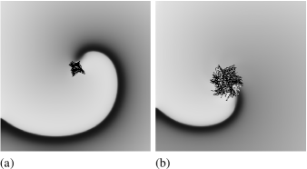
Figure 1: Snapshots of anticlockwise rotating spiral waves of electrical excitation, together with traces of their tips, in a reaction-diffusion model of guinea pig ventricular tissue, (a) classical meander in a model with standard parameters Biktashev and Holden (1996), (b) hypermeander in the same model with parameters changed to represent Long QT syndrome Biktashev and Holden (1998a).

The equations of motion of the meandering spiral tip

may be derived by the standard procedure of rewriting the underlying partial differential equations as a skew product Barkley (1994); Fiedler et al. (1996); Biktashev et al. (1996); Sandstede et al. (1997); Biktashev and Holden (1998b); Golubitsky et al. (2000); Nicol et al. (2001); Ashwin et al. (2001); Roberts et al. (2002); Beyn and Thümmler (2004); Foulkes and Biktashev (2010); Hermann and Gottwald (2010); Gottwald and Melbourne (2013). Consider the ${\color[rgb]{0,0,1}\ell}$-component reaction-diffusion system on the plane,

$$\partial_{\color[rgb]{0,0,1}t}{\color[rgb]{0,0,1}u}={\color[rgb]{0,0,1}D}\nabla^{2}{\color[rgb]{0,0,1}u}+{\color[rgb]{0,0,1}f}({\color[rgb]{0,0,1}u}),\quad{\color[rgb]{0,0,1}u}({\color[rgb]{0,0,1}\mathbf{r}},{\color[rgb]{0,0,1}t})\in\mathbb{R}^{\color[rgb]{0,0,1}\ell},\quad{\color[rgb]{0,0,1}\mathbf{r}}\in\mathbb{R}^{2},$$

as a flow in the phase space which is an infinite-dimensional space of functions $\mathbb{R}^{2}\to\mathbb{R}^{\color[rgb]{0,0,1}\ell}$. The symmetry group is the Euclidean group ${\color[rgb]{0,0,1}\mathcal{G}}$ of transformations of the plane ${\color[rgb]{0,0,1}g}:\mathbb{R}^{2}\to\mathbb{R}^{2}$ acting on $\mathbb{R}^{2}$ by translations and rotations and thereby acting on functions ${\color[rgb]{0,0,1}u}:\mathbb{R}^{2}\to\mathbb{R}^{\color[rgb]{0,0,1}\ell}$ by ${\color[rgb]{0,0,1}u}({\color[rgb]{0,0,1}\mathbf{r}})\mapsto{\color[rgb]{0,0,1}u}({\color[rgb]{0,0,1}g}^{-1}{\color[rgb]{0,0,1}\mathbf{r}})$.

Such systems with symmetry, or “equivariant dynamical systems” can be cast into a skew product form

$$\dot{\color[rgb]{0,0,1}X}={\color[rgb]{0,0,1}\eta}({\color[rgb]{0,0,1}X}),\qquad\dot{\color[rgb]{0,0,1}g}={\color[rgb]{0,0,1}g}{\color[rgb]{0,0,1}\xi}({\color[rgb]{0,0,1}X}),$$

on ${\color[rgb]{0,0,1}\mathcal{X}}\times{\color[rgb]{0,0,1}\mathcal{G}}$, where the dynamics on the symmetry group ${\color[rgb]{0,0,1}\mathcal{G}}$ is driven by the “shape dynamics” on a cross-section ${\color[rgb]{0,0,1}\mathcal{X}}$ transverse to the group directions. Here, ${\color[rgb]{0,0,1}g}{\color[rgb]{0,0,1}\xi}({\color[rgb]{0,0,1}X})$ denotes the action of the group element ${\color[rgb]{0,0,1}g}\in{\color[rgb]{0,0,1}\mathcal{G}}$ on vectors ${\color[rgb]{0,0,1}\xi}({\color[rgb]{0,0,1}X})$ lying in the Lie algebra of ${\color[rgb]{0,0,1}\mathcal{G}}$; ${\color[rgb]{0,0,1}\eta}$ and ${\color[rgb]{0,0,1}\xi}$ are defined by components of the vector field along ${\color[rgb]{0,0,1}\mathcal{X}}$ and orbits of ${\color[rgb]{0,0,1}\mathcal{G}}$ respectively.

The shape dynamics $\dot{\color[rgb]{0,0,1}X}={\color[rgb]{0,0,1}\eta}({\color[rgb]{0,0,1}X})$ on the cross-section ${\color[rgb]{0,0,1}\mathcal{X}}$ is a dynamical system devoid of symmetries. Substituting the solution ${\color[rgb]{0,0,1}X}({\color[rgb]{0,0,1}t})$ for the shape dynamics into the $\dot{\color[rgb]{0,0,1}g}$ equation yields the nonautonomous finite-dimensional equation $\dot{\color[rgb]{0,0,1}g}={\color[rgb]{0,0,1}g}{\color[rgb]{0,0,1}\xi}({\color[rgb]{0,0,1}X}({\color[rgb]{0,0,1}t}))$ to be solved for the group dynamics.

For the Euclidean group ${\color[rgb]{0,0,1}\mathcal{G}}$ consisting of planar translations ${\color[rgb]{0,0,1}p}$ and rotations ${\color[rgb]{0,0,1}\varphi}$, the equations become

$$\dot{\color[rgb]{0,0,1}X}={\color[rgb]{0,0,1}\eta}({\color[rgb]{0,0,1}X}),\qquad\dot{\color[rgb]{0,0,1}\varphi}={\color[rgb]{0,0,1}h}({\color[rgb]{0,0,1}X}),\qquad\dot{\color[rgb]{0,0,1}p}={\color[rgb]{0,0,1}v}({\color[rgb]{0,0,1}X})\;e^{i{\color[rgb]{0,0,1}\varphi}}.$$ (1)

The variables ${\color[rgb]{0,0,1}p}$ and ${\color[rgb]{0,0,1}\varphi}$ can be interpreted as position and orientation of the tip of the spiral, then ${\color[rgb]{0,0,1}X}({\color[rgb]{0,0,1}t})$ describes the evolution in the frame comoving with the tip Biktashev et al. (1996); Foulkes and Biktashev (2010). Standard low-dimensional attractors in ${\color[rgb]{0,0,1}\mathcal{X}}$ produce the classical tip meandering patterns through the $\dot{\color[rgb]{0,0,1}p}$ equation, namely an equilibrium produces stationary rotation, a limit cycle produces the two-frequency flower-pattern meander, and more complicated attractors produce “hypermeander”. Hypermeander produced by chaotic base dynamics is asymptotically a deterministic Brownian motion Biktashev and Holden (1998b); Nicol et al. (2001). Quasiperiodic base dynamics produce another kind of hypermeander, with tip trajectories almost certainly bounded, but exhibiting unlimited directed motion at a dense set of parameter values Nicol et al. (2001). Similar dynamics may be observed when a spiral with two-periodic meander is subject to periodic external forcing Mantel and Barkley (1996).

Our aim is to characterize the size of a quasiperiodic meandering trajectory when it is finite.

The mathematical problem.

We assume ${\color[rgb]{0,0,1}m}$-frequency quasiperiodic dynamics in the base system, ${\color[rgb]{0,0,1}m}\geq 2$, with ${\color[rgb]{0,0,1}X}={\color[rgb]{0,0,1}\theta}\in\mathbb{T}^{\color[rgb]{0,0,1}m}=(\mathbb{R}/2\pi\mathbb{Z})^{\color[rgb]{0,0,1}m}$ being coordinates on the invariant ${\color[rgb]{0,0,1}m}$-torus, so that the shape dynamics $\dot{\color[rgb]{0,0,1}X}={\color[rgb]{0,0,1}\eta}({\color[rgb]{0,0,1}X})$ becomes

$$\dot{\color[rgb]{0,0,1}\theta}={\color[rgb]{0,0,1}\omega},$$ (2)

where ${\color[rgb]{0,0,1}\omega}\in\mathbb{R}^{\color[rgb]{0,0,1}m}$ is a set of irrationally related frequencies . The $\dot{\color[rgb]{0,0,1}g}$ equations become

$$\dot{\color[rgb]{0,0,1}\varphi}={\color[rgb]{0,0,1}h}({\color[rgb]{0,0,1}\theta}),\qquad\dot{\color[rgb]{0,0,1}p}={\color[rgb]{0,0,1}v}({\color[rgb]{0,0,1}\theta})\;e^{i{\color[rgb]{0,0,1}\varphi}}.$$ (3)

Equations (2,3) comprise a closed system describing the trajectory of the quasiperiodic meandering spiral tip.

The $\mathbb{R}^{1}$-extension of the quasiperiodic dynamics.

First we illustrate our main idea for the simpler case where the orientation angle ${\color[rgb]{0,0,1}\varphi}$ is absent and the position ${\color[rgb]{0,0,1}p}$ is one-dimensional. The shape dynamics remains as in (2) with ${\color[rgb]{0,0,1}\theta}\in\mathbb{T}^{\color[rgb]{0,0,1}k}$, ${\color[rgb]{0,0,1}k}\geq 2$. Then a point with coordinate ${\color[rgb]{0,0,1}p}\in\mathbb{R}^{1}$ moves according to

$$\dot{\color[rgb]{0,0,1}p}={\color[rgb]{0,0,1}s}({\color[rgb]{0,0,1}\theta})=\sum\limits_{{\color[rgb]{0,0,1}n}\in\mathbb{Z}^{\color[rgb]{0,0,1}k}}{\color[rgb]{0,0,1}s}_{\color[rgb]{0,0,1}n}e^{i{\color[rgb]{0,0,1}n}\cdot{\color[rgb]{0,0,1}\theta}},\qquad\dot{\color[rgb]{0,0,1}\theta}={\color[rgb]{0,0,1}\omega}.$$ (4)

Termwise integration gives

$${\color[rgb]{0,0,1}p}({\color[rgb]{0,0,1}t})={\color[rgb]{0,0,1}p}(0)+{\color[rgb]{0,0,1}s}_{0}{\color[rgb]{0,0,1}t}+\sideset{}{{}^{\prime}}{\sum}\limits_{{\color[rgb]{0,0,1}n}\in\mathbb{Z}^{\color[rgb]{0,0,1}k}}\frac{-i{\color[rgb]{0,0,1}s}_{\color[rgb]{0,0,1}n}}{{\color[rgb]{0,0,1}n}\cdot{\color[rgb]{0,0,1}\omega}}\left(e^{i{\color[rgb]{0,0,1}n}\cdot{\color[rgb]{0,0,1}\omega}{\color[rgb]{0,0,1}t}}-1\right),$$

where the prime denotes summation over ${\color[rgb]{0,0,1}n}\neq 0$. Consider the infinite sum here, defining the deviation of ${\color[rgb]{0,0,1}p}$ from steady motion, ${\color[rgb]{0,0,1}\Delta}_{\color[rgb]{0,0,1}t}({\color[rgb]{0,0,1}\omega})={\color[rgb]{0,0,1}p}({\color[rgb]{0,0,1}t})-{\color[rgb]{0,0,1}p}(0)-{\color[rgb]{0,0,1}s}_{0}{\color[rgb]{0,0,1}t}$. For an arbitrarily chosen ${\color[rgb]{0,0,1}\omega}$, its components are almost certainly incommensurate, and, moreover, Diophantine. So the denominators in the infinite sum are nonzero, but many of them are very small; nevertheless they decay slowly with $\left\lVert{\color[rgb]{0,0,1}n}\right\rVert=\left({\color[rgb]{0,0,1}n}_{1}^{2}+\dots+{\color[rgb]{0,0,1}n}_{\color[rgb]{0,0,1}k}^{2}\right)^{1/2}$. This is compensated by the fact that if the function ${\color[rgb]{0,0,1}s}({\color[rgb]{0,0,1}\theta})$ is sufficiently smooth, its Fourier coefficients ${\color[rgb]{0,0,1}s}_{\color[rgb]{0,0,1}n}$ in the numerators quickly decay with $\left\lVert{\color[rgb]{0,0,1}n}\right\rVert$. As a result, the infinite sum remains bounded for ${\color[rgb]{0,0,1}t}\geq 0$, for ${\color[rgb]{0,0,1}s}({\color[rgb]{0,0,1}\theta})$ sufficiently smooth and almost all ${\color[rgb]{0,0,1}\omega}$ Nicol et al. (2001).

So if we consider the trajectories in the frame moving with the velocity ${\color[rgb]{0,0,1}s}_{0}$, we know they are typically confined to a finite space. Now we ask how large they can be. The size of a finite piece of trajectory may be measured in various ways, say by the departure from the initial point ${\color[rgb]{0,0,1}\Delta}_{\color[rgb]{0,0,1}t}({\color[rgb]{0,0,1}\omega})={\color[rgb]{0,0,1}p}({\color[rgb]{0,0,1}t})-{\color[rgb]{0,0,1}p}(0)$, its time average, ${\color[rgb]{0,0,1}\mu_{{\color[rgb]{0,0,1}T}}}({\color[rgb]{0,0,1}\omega})={\color[rgb]{0,0,1}T}^{-1}\int_{0}^{\color[rgb]{0,0,1}T}{\color[rgb]{0,0,1}\Delta}_{\color[rgb]{0,0,1}t}({\color[rgb]{0,0,1}\omega})\,\mathrm{d}{\color[rgb]{0,0,1}t}$, and the corresponding variance, ${\color[rgb]{0,0,1}\sigma_{{\color[rgb]{0,0,1}T}}^{2}}({\color[rgb]{0,0,1}\omega})={\color[rgb]{0,0,1}T}^{-1}\int_{0}^{\color[rgb]{0,0,1}T}\left\lvert{\color[rgb]{0,0,1}\Delta}_{\color[rgb]{0,0,1}t}({\color[rgb]{0,0,1}\omega})-{\color[rgb]{0,0,1}\mu_{{\color[rgb]{0,0,1}T}}}({\color[rgb]{0,0,1}\omega})\right\rvert^{2}\,\mathrm{d}{\color[rgb]{0,0,1}t}$. For instance, as ${\color[rgb]{0,0,1}T}\to\infty$ we obtain

$${\color[rgb]{0,0,1}\sigma_{\infty}^{2}}({\color[rgb]{0,0,1}\omega})=\sideset{}{{}^{\prime}}{\sum}\limits_{{\color[rgb]{0,0,1}n}\in\mathbb{Z}^{\color[rgb]{0,0,1}k}}\frac{\left\lvert{\color[rgb]{0,0,1}s}_{{\color[rgb]{0,0,1}n}}\right\rvert^{2}}{({\color[rgb]{0,0,1}n}\cdot{\color[rgb]{0,0,1}\omega})^{2}}.$$ (5)

By the above arguments, for almost any vector ${\color[rgb]{0,0,1}\omega}$, this expression is finite. However, as typically all ${\color[rgb]{0,0,1}s}_{\color[rgb]{0,0,1}n}$ are nonzero, expression (5) is infinite for all ${\color[rgb]{0,0,1}\omega}$ for which the denominator is zero, and for ${\color[rgb]{0,0,1}k}\geq 2$, this is a dense set. That is, the function ${\color[rgb]{0,0,1}\sigma_{\infty}}({\color[rgb]{0,0,1}\omega})$ is almost everywhere defined and finite, but is everywhere discontinuous. The latter property implies that for any physical purpose, questions about the value of the function at a particular point are meaningless, as any uncertainty in the arguments, no matter how small, causes a non-small, in fact infinite, uncertainty in the value of the function.

Hence, a deterministic view on the function ${\color[rgb]{0,0,1}\sigma_{\infty}}({\color[rgb]{0,0,1}\omega})$ is inadequate, and we are forced to adopt a probabilistic view. Suppose we know ${\color[rgb]{0,0,1}\omega}$ approximately, say, its probability density is uniformly distributed in ${\color[rgb]{0,0,1}B}={\color[rgb]{0,0,1}B}_{{\color[rgb]{0,0,1}\delta}}({\color[rgb]{0,0,1}\omega}_{0})$, a ball of radius ${\color[rgb]{0,0,1}\delta}$ centered at ${\color[rgb]{0,0,1}\omega}_{0}$ . The expectation of the trajectory size is then

$$\mathrm{E}\left[{\color[rgb]{0,0,1}\sigma_{\infty}}\right]=\frac{1}{{\color[rgb]{0,0,1}\beta}}\int\limits_{{\color[rgb]{0,0,1}B}}{\color[rgb]{0,0,1}\sigma_{\infty}}({\color[rgb]{0,0,1}\omega})\;\mathrm{d}{\color[rgb]{0,0,1}\omega}=\frac{1}{{\color[rgb]{0,0,1}\beta}}\int\limits_{{\color[rgb]{0,0,1}B}}\left(\sideset{}{{}^{\prime}}{\sum}\limits_{{\color[rgb]{0,0,1}n}\in\mathbb{Z}^{\color[rgb]{0,0,1}k}}\frac{\left\lvert{\color[rgb]{0,0,1}s}_{{\color[rgb]{0,0,1}n}}\right\rvert^{2}}{({\color[rgb]{0,0,1}n}\cdot{\color[rgb]{0,0,1}\omega})^{2}}\right)^{1/2}\mathrm{d}{\color[rgb]{0,0,1}\omega},$$

where ${\color[rgb]{0,0,1}\beta}=\mathop{\mathrm{Vol}}_{{\color[rgb]{0,0,1}k}}({\color[rgb]{0,0,1}B})$. The set of hyperplanes ${\color[rgb]{0,0,1}n}\cdot{\color[rgb]{0,0,1}\omega}=0$, ${\color[rgb]{0,0,1}n}\in\mathbb{Z}^{\color[rgb]{0,0,1}k}$ is dense so there is an infinite set of ${\color[rgb]{0,0,1}n}\in\mathbb{Z}^{\color[rgb]{0,0,1}k}$ whose hyperplanes ${\color[rgb]{0,0,1}n}\cdot{\color[rgb]{0,0,1}\omega}=0$ cut through ${\color[rgb]{0,0,1}B}$. For any such ${\color[rgb]{0,0,1}n}$, we have

$$\mathrm{E}\left[{\color[rgb]{0,0,1}\sigma_{\infty}}\right]\geq\frac{1}{{\color[rgb]{0,0,1}\beta}}\int\limits_{{\color[rgb]{0,0,1}B}}\left\lvert\frac{{\color[rgb]{0,0,1}s}_{{\color[rgb]{0,0,1}n}}}{{\color[rgb]{0,0,1}n}\cdot{\color[rgb]{0,0,1}\omega}}\right\rvert\mathrm{d}{\color[rgb]{0,0,1}\omega}.$$

Then, for some ${\color[rgb]{0,0,1}A},{\color[rgb]{0,0,1}\epsilon}>0$ depending on ${\color[rgb]{0,0,1}n}$, we have

$$\int_{{\color[rgb]{0,0,1}B}}\frac{\mathrm{d}{\color[rgb]{0,0,1}\omega}}{|{\color[rgb]{0,0,1}n}\cdot{\color[rgb]{0,0,1}\omega}|}>{\color[rgb]{0,0,1}A}\int_{-{\color[rgb]{0,0,1}\epsilon}}^{{\color[rgb]{0,0,1}\epsilon}}\,\frac{\mathrm{d}{{\color[rgb]{0,0,1}z}}}{|{\color[rgb]{0,0,1}z}|}=+\infty.$$

Typically, $\left\lvert{\color[rgb]{0,0,1}s}_{{\color[rgb]{0,0,1}n}}\right\rvert>0$ for all such ${\color[rgb]{0,0,1}n}$, therefore we have $\mathrm{E}\left[{\color[rgb]{0,0,1}\sigma_{\infty}}\right]=+\infty$.

That is, the deviation from steady motion is almost certainly finite, but its average expected value is infinite.

The quasiperiodic hypermeander trajectories.

We now return to the equations (2,3) governing quasiperiodic hypermeander. Consider first the $\dot{\color[rgb]{0,0,1}\theta}$, $\dot{\color[rgb]{0,0,1}\varphi}$ subsystem

$$\dot{\color[rgb]{0,0,1}\theta}={\color[rgb]{0,0,1}\omega},\qquad\dot{\color[rgb]{0,0,1}\varphi}={\color[rgb]{0,0,1}h}({\color[rgb]{0,0,1}\theta}).$$ (6)

This has the form of (4) with ${\color[rgb]{0,0,1}k}={\color[rgb]{0,0,1}m}$, ${\color[rgb]{0,0,1}p}={\color[rgb]{0,0,1}\varphi}$, ${\color[rgb]{0,0,1}s}={\color[rgb]{0,0,1}h}$. Proceeding as for $\mathbb{R}^{1}$-extensions, we obtain ${\color[rgb]{0,0,1}\varphi}={\color[rgb]{0,0,1}\varphi}_{0}+{\color[rgb]{0,0,1}h}_{0}{\color[rgb]{0,0,1}t}+{\color[rgb]{0,0,1}\Phi}({\color[rgb]{0,0,1}\theta})$, where ${\color[rgb]{0,0,1}\Phi}({\color[rgb]{0,0,1}\theta})=-i\sideset{}{{}^{\prime}}{\sum}_{{\color[rgb]{0,0,1}n}\in\mathbb{Z}^{\color[rgb]{0,0,1}m}}{\color[rgb]{0,0,1}h}_{\color[rgb]{0,0,1}n}\left(e^{i{\color[rgb]{0,0,1}n}\cdot{\color[rgb]{0,0,1}\theta}}-1\right)/{\color[rgb]{0,0,1}n}\cdot{\color[rgb]{0,0,1}\omega}$. Substituting into the $\dot{\color[rgb]{0,0,1}p}$ equation, we obtain

$$\dot{\color[rgb]{0,0,1}p}={\color[rgb]{0,0,1}v}({\color[rgb]{0,0,1}\theta})e^{i{\color[rgb]{0,0,1}\varphi}_{0}+{\color[rgb]{0,0,1}\Phi}({\color[rgb]{0,0,1}\theta})}e^{i{\color[rgb]{0,0,1}h}_{0}{\color[rgb]{0,0,1}t}}={\color[rgb]{0,0,1}v}({\color[rgb]{0,0,1}\theta})e^{i({\color[rgb]{0,0,1}\varphi}_{0}+{\color[rgb]{0,0,1}\Phi}({\color[rgb]{0,0,1}\theta})+{\color[rgb]{0,0,1}\theta}_{{\color[rgb]{0,0,1}m}+1})},$$

where ${\color[rgb]{0,0,1}\theta}_{{\color[rgb]{0,0,1}m}+1}\in\mathbb{T}^{1}$ satisfies the equation $\dot{\color[rgb]{0,0,1}\theta}_{{\color[rgb]{0,0,1}m}+1}={\color[rgb]{0,0,1}h}_{0}$. Hence the evolution of $\dot{\color[rgb]{0,0,1}p}$ is governed by the skew product equations

$$\dot{\color[rgb]{0,0,1}\tilde{{\color[rgb]{0,0,1}\theta}}}={\color[rgb]{0,0,1}\tilde{{\color[rgb]{0,0,1}\omega}}},\qquad\dot{\color[rgb]{0,0,1}p}={\color[rgb]{0,0,1}\tilde{v}}({\color[rgb]{0,0,1}\tilde{{\color[rgb]{0,0,1}\theta}}}),$$ (7)

where ${\color[rgb]{0,0,1}\tilde{{\color[rgb]{0,0,1}\omega}}}=({\color[rgb]{0,0,1}\omega},{\color[rgb]{0,0,1}h}_{0})\in\mathbb{R}^{{\color[rgb]{0,0,1}m}+1}$, ${\color[rgb]{0,0,1}\tilde{{\color[rgb]{0,0,1}\theta}}}=({\color[rgb]{0,0,1}\theta},{\color[rgb]{0,0,1}{\color[rgb]{0,0,1}\theta}_{{\color[rgb]{0,0,1}m}+1}})\in\mathbb{T}^{{\color[rgb]{0,0,1}m}+1}$ and

$${\color[rgb]{0,0,1}\tilde{v}}({\color[rgb]{0,0,1}\tilde{{\color[rgb]{0,0,1}\theta}}})={\color[rgb]{0,0,1}v}({\color[rgb]{0,0,1}\theta})\,e^{i({\color[rgb]{0,0,1}\varphi}_{0}+{\color[rgb]{0,0,1}\Phi}({\color[rgb]{0,0,1}\theta})+{\color[rgb]{0,0,1}{\color[rgb]{0,0,1}\theta}_{{\color[rgb]{0,0,1}m}+1}})}.$$ (8)

System (7) has a similar form to (4) (separately for the real and imaginary parts of ${\color[rgb]{0,0,1}p}$), except that now ${\color[rgb]{0,0,1}k}={\color[rgb]{0,0,1}m}+1$, ${\color[rgb]{0,0,1}\theta}\in\mathbb{T}^{\color[rgb]{0,0,1}m}$ and ${\color[rgb]{0,0,1}\tilde{{\color[rgb]{0,0,1}\theta}}}\in\mathbb{T}^{{\color[rgb]{0,0,1}m}+1}$ Also, we notice that due to (8), Fourier components ${\color[rgb]{0,0,1}\tilde{v}}_{\color[rgb]{0,0,1}n}$ are nonzero only for ${\color[rgb]{0,0,1}n}_{{\color[rgb]{0,0,1}m}+1}=\pm 1$, which implies that ${\color[rgb]{0,0,1}\tilde{v}}_{0}=0$. Physically speaking, due to the rotation of the meandering tip, its average spatial velocity is always zero. Hence, the function ${\color[rgb]{0,0,1}\sigma_{\infty}}({\color[rgb]{0,0,1}\tilde{{\color[rgb]{0,0,1}\omega}}})$ in this case is just the size of the trajectory, defined as the root mean square of the distance of the tip from the centroid of the trajectory.

Based on the results of the previous paragraph, we conclude from here our main result: for hypermeandering spirals, the long-term average of the displacement of the tip from its centroid is a random quantity, which takes finite values with probability one, but has an infinite expectation. This result is proved rigorously in Biktashev and Melbourne (2020). The rest of our results below are at the physical level of rigour.

The asymptotic distribution of the trajectory size

is fairly generic for typical systems. Consider when the trajectory size

$${\color[rgb]{0,0,1}\sigma_{\infty}}({\color[rgb]{0,0,1}\tilde{{\color[rgb]{0,0,1}\omega}}})=\left(\sideset{}{{}^{\prime}}{\sum}\limits_{{\color[rgb]{0,0,1}n}\in\mathbb{Z}^{{\color[rgb]{0,0,1}m}+1}}\frac{\left\lvert{\color[rgb]{0,0,1}v}_{{\color[rgb]{0,0,1}n}}({\color[rgb]{0,0,1}\tilde{{\color[rgb]{0,0,1}\omega}}})\right\rvert^{2}}{({\color[rgb]{0,0,1}n}\cdot{\color[rgb]{0,0,1}\tilde{{\color[rgb]{0,0,1}\omega}}})^{2}}\right)^{1/2}$$ (9)

is large. This requires that at least one of the terms in the infinite sum is large. It is most likely that the largest term by far exceeds all the others. So, the tail of the distribution of ${\color[rgb]{0,0,1}\sigma_{\infty}}$ can be understood via the distribution of individual terms ${\color[rgb]{0,0,1}S}_{\color[rgb]{0,0,1}n}({\color[rgb]{0,0,1}\tilde{{\color[rgb]{0,0,1}\omega}}})=\left\lvert{\color[rgb]{0,0,1}v}_{{\color[rgb]{0,0,1}n}}({\color[rgb]{0,0,1}\tilde{{\color[rgb]{0,0,1}\omega}}})\right\rvert^{2}/({\color[rgb]{0,0,1}n}\cdot{\color[rgb]{0,0,1}\tilde{{\color[rgb]{0,0,1}\omega}}})^{2}$. Clearly, $\mathbb{P}\left[{\color[rgb]{0,0,1}S}_{\color[rgb]{0,0,1}n}>{\color[rgb]{0,0,1}x}^{2}\right]\propto{\color[rgb]{0,0,1}x}^{-1}$ as ${\color[rgb]{0,0,1}x}\to+\infty$ as long as $\{{\color[rgb]{0,0,1}n}\cdot{\color[rgb]{0,0,1}\tilde{{\color[rgb]{0,0,1}\omega}}}=0\}\cap{\color[rgb]{0,0,1}B}\neq\emptyset$, and the distribution of ${\color[rgb]{0,0,1}\sigma_{\infty}}$ corresponds to the distribution of the square root of the largest of such terms. Hence, for a typical continuous distribution of ${\color[rgb]{0,0,1}\tilde{{\color[rgb]{0,0,1}\omega}}}$, we expect

$${\color[rgb]{0,0,1}F}({\color[rgb]{0,0,1}x})\equiv\mathbb{P}\left[{\color[rgb]{0,0,1}\sigma_{\infty}}>{\color[rgb]{0,0,1}x}\right]\propto{\color[rgb]{0,0,1}x}^{-1},\quad\textrm{as}\quad{\color[rgb]{0,0,1}x}\to+\infty.$$ (10)

Growth rate of the trajectory size.

In practice we can observe the trajectory only for a finite, even if large, time interval ${\color[rgb]{0,0,1}T}$. Let us see how the expectation of the trajectory size grows with ${\color[rgb]{0,0,1}T}$. Consider, for instance, the departure from the initial point, ${\color[rgb]{0,0,1}\Delta}_{\color[rgb]{0,0,1}T}$. The exact expression for its square is

$$\left\lvert{\color[rgb]{0,0,1}\Delta}_{\color[rgb]{0,0,1}T}({\color[rgb]{0,0,1}\tilde{{\color[rgb]{0,0,1}\omega}}})\right\rvert^{2} =\sideset{}{{}^{\prime}}{\sum}\limits_{{\color[rgb]{0,0,1}{\color[rgb]{0,0,1}n}^{\prime}},{\color[rgb]{0,0,1}{\color[rgb]{0,0,1}n}^{\prime\prime}}\in\mathbb{Z}^{{\color[rgb]{0,0,1}m}+1}}\frac{{{\color[rgb]{0,0,1}v}}^{*}_{{\color[rgb]{0,0,1}{\color[rgb]{0,0,1}n}^{\prime}}}{\color[rgb]{0,0,1}v}_{{\color[rgb]{0,0,1}{\color[rgb]{0,0,1}n}^{\prime\prime}}}}{({\color[rgb]{0,0,1}{\color[rgb]{0,0,1}n}^{\prime}}\cdot{\color[rgb]{0,0,1}\tilde{{\color[rgb]{0,0,1}\omega}}})({\color[rgb]{0,0,1}{\color[rgb]{0,0,1}n}^{\prime\prime}}\cdot{\color[rgb]{0,0,1}\tilde{{\color[rgb]{0,0,1}\omega}}})}$$

$$\mbox{}\times\left(e^{-i{\color[rgb]{0,0,1}{\color[rgb]{0,0,1}n}^{\prime}}\cdot{\color[rgb]{0,0,1}\tilde{{\color[rgb]{0,0,1}\omega}}}{\color[rgb]{0,0,1}T}}-1\right)\left(e^{i{\color[rgb]{0,0,1}{\color[rgb]{0,0,1}n}^{\prime\prime}}\cdot{\color[rgb]{0,0,1}\tilde{{\color[rgb]{0,0,1}\omega}}}{\color[rgb]{0,0,1}T}}-1\right).$$

Secular growth of the expectation of this series is due to resonant terms, i.e. those with ${\color[rgb]{0,0,1}{\color[rgb]{0,0,1}n}^{\prime}}$ parallel to ${\color[rgb]{0,0,1}{\color[rgb]{0,0,1}n}^{\prime\prime}}$. If ${\color[rgb]{0,0,1}\tilde{v}}({\color[rgb]{0,0,1}\tilde{{\color[rgb]{0,0,1}\omega}}})$ is smooth and ${\color[rgb]{0,0,1}v}_{\color[rgb]{0,0,1}n}$ quickly decay, then the main contribution is by principal resonances ${\color[rgb]{0,0,1}{\color[rgb]{0,0,1}n}^{\prime}}={\color[rgb]{0,0,1}{\color[rgb]{0,0,1}n}^{\prime\prime}}$. This gives an approximation

$$\left\lvert{\color[rgb]{0,0,1}\Delta}_{\color[rgb]{0,0,1}T}\right\rvert^{2}\approx\sideset{}{{}^{\prime}}{\sum}\limits_{{\color[rgb]{0,0,1}n}\in\mathbb{Z}^{{\color[rgb]{0,0,1}m}+1}}\frac{2\left\lvert{\color[rgb]{0,0,1}v}_{{\color[rgb]{0,0,1}n}}\right\rvert^{2}}{({\color[rgb]{0,0,1}n}\cdot{\color[rgb]{0,0,1}\tilde{{\color[rgb]{0,0,1}\omega}}})^{2}}\left[1-\cos\left({\color[rgb]{0,0,1}n}\cdot{\color[rgb]{0,0,1}\tilde{{\color[rgb]{0,0,1}\omega}}}{\color[rgb]{0,0,1}T}\right)\right].$$

To evaluate the corresponding expectation,

$$\mathrm{E}\left[\left\lvert{\color[rgb]{0,0,1}\Delta}_{\color[rgb]{0,0,1}T}\right\rvert^{2}\right]=\frac{1}{{\color[rgb]{0,0,1}\beta}}\int\limits_{{\color[rgb]{0,0,1}\tilde{{\color[rgb]{0,0,1}\omega}}}\in{\color[rgb]{0,0,1}B}}\left\lvert{\color[rgb]{0,0,1}\Delta}_{\color[rgb]{0,0,1}T}\right\rvert^{2}\,\mathrm{d}{\color[rgb]{0,0,1}\tilde{{\color[rgb]{0,0,1}\omega}}},$$

where ${\color[rgb]{0,0,1}\beta}=\mathop{\mathrm{Vol}}_{{\color[rgb]{0,0,1}m}+1}({\color[rgb]{0,0,1}B})$, we substitute ${\color[rgb]{0,0,1}z}={\color[rgb]{0,0,1}n}\cdot{\color[rgb]{0,0,1}\tilde{{\color[rgb]{0,0,1}\omega}}}{\color[rgb]{0,0,1}T}$ and let ${\color[rgb]{0,0,1}\chi}_{\color[rgb]{0,0,1}n}=\mathop{\mathrm{Vol}}_{{\color[rgb]{0,0,1}m}}\left(\{{\color[rgb]{0,0,1}\tilde{{\color[rgb]{0,0,1}\omega}}}\,|\,{\color[rgb]{0,0,1}n}\cdot{\color[rgb]{0,0,1}\tilde{{\color[rgb]{0,0,1}\omega}}}=0\}\cap{\color[rgb]{0,0,1}B}\right)$. This leads to

$$\mathrm{E}\left[{\color[rgb]{0,0,1}\Delta}_{\color[rgb]{0,0,1}T}^{2}\right]\approx{\color[rgb]{0,0,1}C}_{1}{\color[rgb]{0,0,1}T},\quad{\color[rgb]{0,0,1}C}_{1}=\frac{2\pi}{{\color[rgb]{0,0,1}\beta}}\sideset{}{{}^{\prime}}{\sum}\limits_{{\color[rgb]{0,0,1}n}\in\mathbb{Z}^{{\color[rgb]{0,0,1}m}+1}}\frac{\left\lvert{\color[rgb]{0,0,1}v}_{{\color[rgb]{0,0,1}n}}\right\rvert^{2}{\color[rgb]{0,0,1}\chi}_{{\color[rgb]{0,0,1}n}}}{\left\lVert{\color[rgb]{0,0,1}n}\right\rVert}.$$ (11)

Detailed calculations are given in the Supplementary materials, where we also show that under similar assumptions,

$$\mathrm{E}\left[{\color[rgb]{0,0,1}\sigma_{{\color[rgb]{0,0,1}T}}^{2}}\right]\approx{\color[rgb]{0,0,1}C}_{2}{\color[rgb]{0,0,1}T},\quad{\color[rgb]{0,0,1}C}_{2}=\frac{\pi}{3{\color[rgb]{0,0,1}\beta}}\sideset{}{{}^{\prime}}{\sum}\limits_{{\color[rgb]{0,0,1}n}\in\mathbb{Z}^{{\color[rgb]{0,0,1}m}+1}}\frac{\left\lvert{\color[rgb]{0,0,1}v}_{{\color[rgb]{0,0,1}n}}\right\rvert^{2}{\color[rgb]{0,0,1}\chi}_{{\color[rgb]{0,0,1}n}}}{\left\lVert{\color[rgb]{0,0,1}n}\right\rVert}.$$ (12)

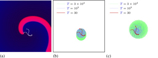
Figure 2: (colour online) (a) Spiral wave and a piece of meander tip trajectory in FitzHugh-Nagumo model (13). (b) Longer pieces of the same tip trajectory. (c) Pieces of trajectory of different lengths generated by the caricature model (14) for ${\color[rgb]{0,0,1}\omega}_{2}=0.49777$.

Numerical illustration.

Fig. 2(a) shows a snapshot of a spiral wave solution, together with a piece of the corresponding tip trajectory, for the FitzHugh-Nagumo model ,

$$u_{\color[rgb]{0,0,1}t}=20(u-u^{3}/3-v)+\nabla^{2}u,$$

$$v_{\color[rgb]{0,0,1}t}=0.05(u+1.2-0.5v).$$ (13)

Fig. 2(b) shows longer pieces of the tip trajectory, which illustrates the key feature of hypermeander: the area occupied by the trajectory can keep growing for a very long time. We have crudely emulated these dynamics by a system (1,2,3) with

$${\color[rgb]{0,0,1}m}=2,\quad{\color[rgb]{0,0,1}v}({\color[rgb]{0,0,1}\theta})=\left(0.6-0.2\beta-0.2\alpha\beta\right)^{-1}-1,$$

$${\color[rgb]{0,0,1}h}({\color[rgb]{0,0,1}\theta})=\left(0.675+0.1\alpha+0.05\beta+0.5\alpha^{2}+0.5\alpha\beta\right.$$

$$\hskip 30.00005pt\left.\mbox{}+0.2\alpha^{3}+0.6\alpha^{2}\beta\right)^{-1}-1,$$

$$\alpha=\cos({\color[rgb]{0,0,1}\theta}_{1})+0.05\tanh(30\cos({\color[rgb]{0,0,1}\theta}_{2})),\quad\beta=\sin({\color[rgb]{0,0,1}\theta}_{1}),$$

$${\color[rgb]{0,0,1}\omega}_{1}=0.354,\quad{\color[rgb]{0,0,1}\omega}_{2}\in[0.475,0.525].$$ (14)

This was done in the spirit of Ashwin et al. (2001) with the base dynamics replaced by an explicit two-periodic flow, but with the view to (i) mimic the actual meander pattern in the PDE model, and (ii) provide sufficient nonlinearity to ensure abundance of combination harmonics in (9). Fig. 2(c) shows pieces of a trajectory of this “caricature” model. One can see the same key feature, that the apparent size of the trajectory very much depends on the interval of observation; however the details are very sensitive to the choice of parameters, including ${\color[rgb]{0,0,1}\omega}_{2}$.

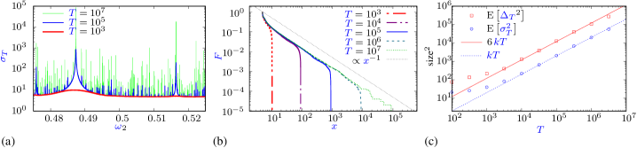
Figure 3: (colour online)(a) Sizes ${\color[rgb]{0,0,1}\sigma_{{\color[rgb]{0,0,1}T}}}$ of trajectories of different length ${\color[rgb]{0,0,1}T}$, as functions of ${\color[rgb]{0,0,1}\omega}_{2}$, semilog plot. (b) Distribution functions ${\color[rgb]{0,0,1}F}({\color[rgb]{0,0,1}x})=\mathbb{P}\left[{\color[rgb]{0,0,1}\sigma_{{\color[rgb]{0,0,1}T}}}({\color[rgb]{0,0,1}\omega}_{2})>{\color[rgb]{0,0,1}x}\right]$, for the trajectory sizes ${\color[rgb]{0,0,1}\sigma_{{\color[rgb]{0,0,1}T}}}$ for lengths ${\color[rgb]{0,0,1}T}$, log-log plot. The straight line is the asymptotic (10). (c) Mean square of trajectory size as function of the time interval, log-log plot. The straight lines are the asymptotics (11) and (12) with a fitted ${\color[rgb]{0,0,1}k}={\color[rgb]{0,0,1}C}_{2}={\color[rgb]{0,0,1}C}_{1}/6$.

Fig. 3(a) illustrates the approach of ${\color[rgb]{0,0,1}\sigma_{{\color[rgb]{0,0,1}T}}}({\color[rgb]{0,0,1}\omega}_{2})$ to an everywhere discontinuous function as ${\color[rgb]{0,0,1}T}\to\infty$. This was obtained for $10^{5}$ values of ${\color[rgb]{0,0,1}\omega}_{2}$ randomly chosen in the shown interval. For smaller ${\color[rgb]{0,0,1}T}$ one can see well shaped individual peaks associated with the poles of ${\color[rgb]{0,0,1}\sigma_{\infty}}({\color[rgb]{0,0,1}\omega}_{2})$ corresponding to the resonances with the highest ${\color[rgb]{0,0,1}v}_{{\color[rgb]{0,0,1}n}}$; for larger ${\color[rgb]{0,0,1}T}$, more of such peaks become pronounced, and they grow stronger. Fig. 3(b) shows the empirical distribution of the trajectory sizes for the pieces of trajectories of the same $10^{5}$ simulations, of different lengths. We see that for larger ${\color[rgb]{0,0,1}T}$, the distribution approaches the theoretical prediction (10). Finally, fig. 3(c) shows the growth of two empirical estimates of trajectory size with time, in agreement with (12) and (11), including the predicted approximate ratio of 6 between them.

In conclusion,

quasiperiodic hypermeander of spiral waves has paradoxical properties. Even though described by deterministic equations, with no chaos involved, the question of the size of the tip trajectory does not have a meaningful deterministic answer and requires probabilistic treatment. In probabilistic terms, although the tip trajectory is confined with probability one, the expectation of its size, however measured, is infinite. There it is similar to the “St. Petersburg lottery”, in which a win is almost certainly finite, but its expectation is infinite Bernoulli (1738); Sommer (1954). The realistic price for a ticket in this lottery is nevertheless finite and modest; the resolution of this pardox relevant to us is that high wins require unrealistically long games (Feller, 1968, Section X.4). In our case, the dependence of the trajectory size, whether defined via mean square displacement $\left\lvert{\color[rgb]{0,0,1}\Delta}_{\color[rgb]{0,0,1}T}\right\rvert^{2}$ or variance ${\color[rgb]{0,0,1}\sigma_{{\color[rgb]{0,0,1}T}}^{2}}$, on any parameter affecting the frequency ratios becomes more and more irregular as ${\color[rgb]{0,0,1}T}\to\infty$, and the expectations $\mathrm{E}\left[\left\lvert{\color[rgb]{0,0,1}\Delta}_{\color[rgb]{0,0,1}T}\right\rvert^{2}\right]$ and $\mathrm{E}\left[{\color[rgb]{0,0,1}\sigma_{{\color[rgb]{0,0,1}T}}^{2}}\right]$ defined as averages over parameter variations, grow linearly in ${\color[rgb]{0,0,1}T}$ even though the individual trajectories are bounded. Note that this is different from the linear growth for the mean square displacement of chaotically hypermeandering spirals Biktashev and Holden (1998b); Ashwin et al. (2001) which is for averages over initial conditions.

Practical applications of the theory are most evident for re-entrant waves in cardiac tissue, underlying dangerous cardiac arrhythmias. However implications may be also expected in any physics where the theory involves differential equations with quasiperiodic coefficients. One example may be provided by evolution of tracers in quasi-periodic fluid flows Boatto and Pierrehumbert (1999). On a more speculative level, extension from ODEs in time to PDEs in spatial variables may provide insights into properties of quasicrystals Janssen and Janner (2014) or quasiperiodic dissipative structures Subramanian et al. (2016). Note that properties of quasicrystals, among other things, include superlubricity Koren and Duerig (2016) and superconductivity Kamiya et al. (2018), still awaiting full theoretical treatment.

Acknowledgements VNB was supported by EPSRC Grant EP/N014391/1 (UK), NSF Grant PHY-1748958, NIH Grant R25GM067110, and the Gordon and Betty Moore Foundation Grant 2919.01 (USA). IM was supported by European Advanced Grant ERC AdG 320977 (EU).

Appendix A Supplementary material for
“”
by V. N. Biktashev and I. Melbourne

A.1 Details of the derivation of the trajectory size asymptotics

The exact expression for the square of the departure from the initial point is

$$\left\lvert{\color[rgb]{0,0,1}\Delta}_{\color[rgb]{0,0,1}T}({\color[rgb]{0,0,1}\tilde{{\color[rgb]{0,0,1}\omega}}})\right\rvert^{2}=\left\lvert{\color[rgb]{0,0,1}p}({\color[rgb]{0,0,1}T})-{\color[rgb]{0,0,1}p}(0)\right\rvert^{2}=\left\lvert\sideset{}{{}^{\prime}}{\sum}\limits_{{\color[rgb]{0,0,1}n}\in\mathbb{Z}^{{\color[rgb]{0,0,1}m}+1}}\frac{-i{\color[rgb]{0,0,1}v}_{{\color[rgb]{0,0,1}n}}}{{\color[rgb]{0,0,1}n}\cdot{\color[rgb]{0,0,1}\tilde{{\color[rgb]{0,0,1}\omega}}}}\left(e^{i{\color[rgb]{0,0,1}n}\cdot{\color[rgb]{0,0,1}\tilde{{\color[rgb]{0,0,1}\omega}}}{\color[rgb]{0,0,1}T}}-1\right)\right\rvert^{2}.$$

Then for its expectation we have

$$\mathrm{E}\left[\left\lvert{\color[rgb]{0,0,1}\Delta}_{\color[rgb]{0,0,1}T}\right\rvert^{2}\right]=\frac{1}{{\color[rgb]{0,0,1}\beta}}\int\limits_{\color[rgb]{0,0,1}B}\left\lvert{\color[rgb]{0,0,1}\Delta}_{\color[rgb]{0,0,1}T}({\color[rgb]{0,0,1}\tilde{{\color[rgb]{0,0,1}\omega}}})\right\rvert^{2}\,\mathrm{d}{\color[rgb]{0,0,1}\tilde{{\color[rgb]{0,0,1}\omega}}}=\frac{1}{{\color[rgb]{0,0,1}\beta}}\sideset{}{{}^{\prime}}{\sum}\limits_{{\color[rgb]{0,0,1}{\color[rgb]{0,0,1}n}^{\prime}},{\color[rgb]{0,0,1}{\color[rgb]{0,0,1}n}^{\prime\prime}}}{\color[rgb]{0,0,1}v}_{{\color[rgb]{0,0,1}{\color[rgb]{0,0,1}n}^{\prime}}}{{\color[rgb]{0,0,1}v}}^{*}_{{\color[rgb]{0,0,1}{\color[rgb]{0,0,1}n}^{\prime\prime}}}{\color[rgb]{0,0,1}D}_{{\color[rgb]{0,0,1}{\color[rgb]{0,0,1}n}^{\prime}}{\color[rgb]{0,0,1}{\color[rgb]{0,0,1}n}^{\prime\prime}}}({\color[rgb]{0,0,1}T}),$$

where

$${\color[rgb]{0,0,1}D}_{{\color[rgb]{0,0,1}{\color[rgb]{0,0,1}n}^{\prime}}{\color[rgb]{0,0,1}{\color[rgb]{0,0,1}n}^{\prime\prime}}}({\color[rgb]{0,0,1}T})=\int\limits_{\color[rgb]{0,0,1}B}\frac{e^{-i{\color[rgb]{0,0,1}{\color[rgb]{0,0,1}n}^{\prime}}\cdot{\color[rgb]{0,0,1}\tilde{{\color[rgb]{0,0,1}\omega}}}{\color[rgb]{0,0,1}T}}-1}{{\color[rgb]{0,0,1}{\color[rgb]{0,0,1}n}^{\prime}}\cdot{\color[rgb]{0,0,1}\tilde{{\color[rgb]{0,0,1}\omega}}}}\,\frac{e^{i{\color[rgb]{0,0,1}{\color[rgb]{0,0,1}n}^{\prime\prime}}\cdot{\color[rgb]{0,0,1}\tilde{{\color[rgb]{0,0,1}\omega}}}{\color[rgb]{0,0,1}T}}-1}{{\color[rgb]{0,0,1}{\color[rgb]{0,0,1}n}^{\prime\prime}}\cdot{\color[rgb]{0,0,1}\tilde{{\color[rgb]{0,0,1}\omega}}}}\,\mathrm{d}{\color[rgb]{0,0,1}\tilde{{\color[rgb]{0,0,1}\omega}}}.$$

Let us investigate the behaviour of the coefficients ${\color[rgb]{0,0,1}D}_{{\color[rgb]{0,0,1}{\color[rgb]{0,0,1}n}^{\prime}}{\color[rgb]{0,0,1}{\color[rgb]{0,0,1}n}^{\prime\prime}}}({\color[rgb]{0,0,1}T})$ in the limit ${\color[rgb]{0,0,1}T}\to\infty$. We have to consider separately the cases when the two zero-denominator hyperplanes cut or do not cut through ${\color[rgb]{0,0,1}B}$. Recall that ${\color[rgb]{0,0,1}\chi}_{\color[rgb]{0,0,1}n}\equiv\mathop{\mathrm{Vol}}_{{\color[rgb]{0,0,1}m}}\{{\color[rgb]{0,0,1}\tilde{{\color[rgb]{0,0,1}\omega}}}\,|\,{\color[rgb]{0,0,1}\tilde{{\color[rgb]{0,0,1}\omega}}}\in{\color[rgb]{0,0,1}B}\;\&\;{\color[rgb]{0,0,1}n}\cdot{\color[rgb]{0,0,1}\tilde{{\color[rgb]{0,0,1}\omega}}}=0\}$, and $\left\lVert{\color[rgb]{0,0,1}n}\right\rVert\equiv\left(\sum\limits_{{\color[rgb]{0,0,1}j}=1}^{{\color[rgb]{0,0,1}m}+1}{\color[rgb]{0,0,1}n}_{\color[rgb]{0,0,1}j}^{2}\right)^{1/2}$. We write ${\color[rgb]{0,0,1}n}^{\prime}\parallel{\color[rgb]{0,0,1}n}^{\prime\prime}$ when vectors $n^{\prime}$ and $n^{\prime\prime}$ are parallel (linearly dependent), and ${\color[rgb]{0,0,1}n}^{\prime}\nparallel{\color[rgb]{0,0,1}n}^{\prime\prime}$ otherwise.

• For ${\color[rgb]{0,0,1}\chi}_{{\color[rgb]{0,0,1}{\color[rgb]{0,0,1}n}^{\prime}}}=0$, ${\color[rgb]{0,0,1}\chi}_{{\color[rgb]{0,0,1}{\color[rgb]{0,0,1}n}^{\prime\prime}}}=0$, the coefficients are bounded:

  $$\left\lvert{\color[rgb]{0,0,1}D}_{{\color[rgb]{0,0,1}{\color[rgb]{0,0,1}n}^{\prime}}{\color[rgb]{0,0,1}{\color[rgb]{0,0,1}n}^{\prime\prime}}}({\color[rgb]{0,0,1}T})\right\rvert\leq 4{\color[rgb]{0,0,1}\beta}\left(\min\limits_{{\color[rgb]{0,0,1}\tilde{{\color[rgb]{0,0,1}\omega}}}\in{\color[rgb]{0,0,1}B}}\left\lvert{\color[rgb]{0,0,1}{\color[rgb]{0,0,1}n}^{\prime}}\cdot{\color[rgb]{0,0,1}\tilde{{\color[rgb]{0,0,1}\omega}}}\right\rvert\right)^{-1}\left(\min\limits_{{\color[rgb]{0,0,1}\tilde{{\color[rgb]{0,0,1}\omega}}}\in{\color[rgb]{0,0,1}B}}\left\lvert{\color[rgb]{0,0,1}{\color[rgb]{0,0,1}n}^{\prime\prime}}\cdot{\color[rgb]{0,0,1}\tilde{{\color[rgb]{0,0,1}\omega}}}\right\rvert\right)^{-1}=O\left(1\right).$$

• For ${\color[rgb]{0,0,1}\chi}_{{\color[rgb]{0,0,1}{\color[rgb]{0,0,1}n}^{\prime\prime}}}=0$, ${\color[rgb]{0,0,1}\chi}_{{\color[rgb]{0,0,1}{\color[rgb]{0,0,1}n}^{\prime}}}\neq 0$, we use a change of variables in the space $\left\{{\color[rgb]{0,0,1}\tilde{{\color[rgb]{0,0,1}\omega}}}\right\}=\mathbb{R}^{{\color[rgb]{0,0,1}m}+1}$; namely, ${\color[rgb]{0,0,1}z}={\color[rgb]{0,0,1}{\color[rgb]{0,0,1}n}^{\prime}}\cdot{\color[rgb]{0,0,1}\tilde{{\color[rgb]{0,0,1}\omega}}}{\color[rgb]{0,0,1}T}\in\mathbb{R}$, and ${\color[rgb]{0,0,1}\zeta}\in\mathbb{R}^{{\color[rgb]{0,0,1}m}}$ for the unscaled coordinates in ${\color[rgb]{0,0,1}{\color[rgb]{0,0,1}n}^{\prime}}^{\perp}$. In coordinates $({\color[rgb]{0,0,1}z},{\color[rgb]{0,0,1}\zeta})$, the domain ${\color[rgb]{0,0,1}B}$ is stretched in the ${\color[rgb]{0,0,1}z}$ direction and, as ${\color[rgb]{0,0,1}T}\to\infty$, tends to an infinite cylinder with the axis along the ${\color[rgb]{0,0,1}z}$ axis and the base of measure ${\color[rgb]{0,0,1}\chi}_{\color[rgb]{0,0,1}{\color[rgb]{0,0,1}n}^{\prime}}$. This gives

  $$\left\lvert{\color[rgb]{0,0,1}D}_{{\color[rgb]{0,0,1}{\color[rgb]{0,0,1}n}^{\prime}}{\color[rgb]{0,0,1}{\color[rgb]{0,0,1}n}^{\prime\prime}}}({\color[rgb]{0,0,1}T})\right\rvert\leq\left(\min\limits_{{\color[rgb]{0,0,1}\tilde{{\color[rgb]{0,0,1}\omega}}}\in{\color[rgb]{0,0,1}B}}\left\lvert{\color[rgb]{0,0,1}{\color[rgb]{0,0,1}n}^{\prime\prime}}\cdot{\color[rgb]{0,0,1}\tilde{{\color[rgb]{0,0,1}\omega}}}\right\rvert\right)^{-1}\int\limits_{\color[rgb]{0,0,1}B}\left\lvert\frac{e^{i{\color[rgb]{0,0,1}{\color[rgb]{0,0,1}n}^{\prime}}\cdot{\color[rgb]{0,0,1}\tilde{{\color[rgb]{0,0,1}\omega}}}{\color[rgb]{0,0,1}T}}-1}{{\color[rgb]{0,0,1}{\color[rgb]{0,0,1}n}^{\prime}}\cdot{\color[rgb]{0,0,1}\tilde{{\color[rgb]{0,0,1}\omega}}}}\right\rvert\,\mathrm{d}{\color[rgb]{0,0,1}\tilde{{\color[rgb]{0,0,1}\omega}}}=\left(\min\limits_{{\color[rgb]{0,0,1}\tilde{{\color[rgb]{0,0,1}\omega}}}\in{\color[rgb]{0,0,1}B}}\left\lvert{\color[rgb]{0,0,1}{\color[rgb]{0,0,1}n}^{\prime\prime}}\cdot{\color[rgb]{0,0,1}\tilde{{\color[rgb]{0,0,1}\omega}}}\right\rvert\right)^{-1}\iint\limits_{{\color[rgb]{0,0,1}\tilde{{\color[rgb]{0,0,1}\omega}}}\in{\color[rgb]{0,0,1}B}}\left\lvert\frac{e^{i{\color[rgb]{0,0,1}z}}-1}{{\color[rgb]{0,0,1}z}/{\color[rgb]{0,0,1}T}}\right\rvert\frac{\mathrm{d}{\color[rgb]{0,0,1}z}}{\left\lVert{\color[rgb]{0,0,1}{\color[rgb]{0,0,1}n}^{\prime}}\right\rVert{\color[rgb]{0,0,1}T}}\,\mathrm{d}{\color[rgb]{0,0,1}\zeta}$$

  $$=\left(\min\limits_{{\color[rgb]{0,0,1}\tilde{{\color[rgb]{0,0,1}\omega}}}\in{\color[rgb]{0,0,1}B}}\left\lvert{\color[rgb]{0,0,1}{\color[rgb]{0,0,1}n}^{\prime\prime}}\cdot{\color[rgb]{0,0,1}\tilde{{\color[rgb]{0,0,1}\omega}}}\right\rvert\right)^{-1}\frac{{\color[rgb]{0,0,1}\chi}_{{\color[rgb]{0,0,1}{\color[rgb]{0,0,1}n}^{\prime}}}}{\left\lVert{\color[rgb]{0,0,1}{\color[rgb]{0,0,1}n}^{\prime}}\right\rVert}\int\limits_{-O\left({\color[rgb]{0,0,1}T}\right)}^{O\left({\color[rgb]{0,0,1}T}\right)}\left\lvert\frac{e^{i{\color[rgb]{0,0,1}z}}-1}{{\color[rgb]{0,0,1}z}}\right\rvert\,\mathrm{d}{\color[rgb]{0,0,1}z}=O\left(\ln({\color[rgb]{0,0,1}T})\right),$$

  and similarly for ${\color[rgb]{0,0,1}\chi}_{{\color[rgb]{0,0,1}{\color[rgb]{0,0,1}n}^{\prime}}}=0$, ${\color[rgb]{0,0,1}\chi}_{{\color[rgb]{0,0,1}{\color[rgb]{0,0,1}n}^{\prime\prime}}}\neq 0$.

• For ${\color[rgb]{0,0,1}\chi}_{{\color[rgb]{0,0,1}{\color[rgb]{0,0,1}n}^{\prime}}}\neq 0$, ${\color[rgb]{0,0,1}\chi}_{{\color[rgb]{0,0,1}{\color[rgb]{0,0,1}n}^{\prime\prime}}}\neq 0$, and ${\color[rgb]{0,0,1}{\color[rgb]{0,0,1}n}^{\prime}}\nparallel{\color[rgb]{0,0,1}{\color[rgb]{0,0,1}n}^{\prime\prime}}$, we use variables ${\color[rgb]{0,0,1}{\color[rgb]{0,0,1}z}^{\prime}}={\color[rgb]{0,0,1}{\color[rgb]{0,0,1}n}^{\prime}}\cdot{\color[rgb]{0,0,1}\tilde{{\color[rgb]{0,0,1}\omega}}}{\color[rgb]{0,0,1}T}\in\mathbb{R}$, ${\color[rgb]{0,0,1}{\color[rgb]{0,0,1}z}^{\prime\prime}}={\color[rgb]{0,0,1}{\color[rgb]{0,0,1}n}^{\prime\prime}}\cdot{\color[rgb]{0,0,1}\tilde{{\color[rgb]{0,0,1}\omega}}}{\color[rgb]{0,0,1}T}\in\mathbb{R}$, and ${\color[rgb]{0,0,1}\zeta}\in\mathbb{R}^{{\color[rgb]{0,0,1}m}-1}$ for the unscaled coordinates in $\mathop{\mathrm{span}}({\color[rgb]{0,0,1}{\color[rgb]{0,0,1}n}^{\prime}},{\color[rgb]{0,0,1}{\color[rgb]{0,0,1}n}^{\prime\prime}})^{\perp}$. Then

  $${\color[rgb]{0,0,1}D}_{{\color[rgb]{0,0,1}{\color[rgb]{0,0,1}n}^{\prime}}{\color[rgb]{0,0,1}{\color[rgb]{0,0,1}n}^{\prime\prime}}}({\color[rgb]{0,0,1}T})=\iiint\limits_{{\color[rgb]{0,0,1}\tilde{{\color[rgb]{0,0,1}\omega}}}\in{\color[rgb]{0,0,1}B}}\dfrac{e^{-i{\color[rgb]{0,0,1}{\color[rgb]{0,0,1}z}^{\prime}}}-1}{{\color[rgb]{0,0,1}{\color[rgb]{0,0,1}z}^{\prime}}/{\color[rgb]{0,0,1}T}}\,\dfrac{e^{i{\color[rgb]{0,0,1}{\color[rgb]{0,0,1}z}^{\prime\prime}}}-1}{{\color[rgb]{0,0,1}{\color[rgb]{0,0,1}z}^{\prime\prime}}/{\color[rgb]{0,0,1}T}}\,\dfrac{\mathrm{d}{\color[rgb]{0,0,1}{\color[rgb]{0,0,1}z}^{\prime}}\mathrm{d}{\color[rgb]{0,0,1}{\color[rgb]{0,0,1}z}^{\prime\prime}}}{\left\lVert{\color[rgb]{0,0,1}{\color[rgb]{0,0,1}n}^{\prime}}\right\rVert\left\lVert{\color[rgb]{0,0,1}{\color[rgb]{0,0,1}n}^{\prime\prime}}\right\rVert\sin\left(\widehat{{\color[rgb]{0,0,1}{\color[rgb]{0,0,1}n}^{\prime}},{\color[rgb]{0,0,1}{\color[rgb]{0,0,1}n}^{\prime\prime}}}\right){\color[rgb]{0,0,1}T}^{2}}\,\mathrm{d}{\color[rgb]{0,0,1}\zeta}=O\left(1\right).$$

  Here $\widehat{{\color[rgb]{0,0,1}{\color[rgb]{0,0,1}n}^{\prime}},{\color[rgb]{0,0,1}{\color[rgb]{0,0,1}n}^{\prime\prime}}}$ is the angle between vectors ${\color[rgb]{0,0,1}{\color[rgb]{0,0,1}n}^{\prime}}$ and ${\color[rgb]{0,0,1}{\color[rgb]{0,0,1}n}^{\prime\prime}}$.

• For ${\color[rgb]{0,0,1}\chi}_{{\color[rgb]{0,0,1}{\color[rgb]{0,0,1}n}^{\prime}}}\neq 0$, ${\color[rgb]{0,0,1}\chi}_{{\color[rgb]{0,0,1}{\color[rgb]{0,0,1}n}^{\prime\prime}}}\neq 0$, and ${\color[rgb]{0,0,1}{\color[rgb]{0,0,1}n}^{\prime}}\parallel{\color[rgb]{0,0,1}{\color[rgb]{0,0,1}n}^{\prime\prime}}$, we set ${\color[rgb]{0,0,1}{\color[rgb]{0,0,1}n}^{\prime}}={\color[rgb]{0,0,1}\alpha^{\prime}}{\color[rgb]{0,0,1}n}$, ${\color[rgb]{0,0,1}{\color[rgb]{0,0,1}n}^{\prime\prime}}={\color[rgb]{0,0,1}\alpha^{\prime\prime}}{\color[rgb]{0,0,1}n}$, where ${\color[rgb]{0,0,1}n}\in\mathbb{Z}^{{\color[rgb]{0,0,1}m}+1}$ is their GCD vector and ${\color[rgb]{0,0,1}\alpha^{\prime}},{\color[rgb]{0,0,1}\alpha^{\prime\prime}}\in\mathbb{Z}\setminus\{0\}$ (see Proposition 1 below). In this case the hyperplanes ${\color[rgb]{0,0,1}{\color[rgb]{0,0,1}n}^{\prime}}\cdot{\color[rgb]{0,0,1}\tilde{{\color[rgb]{0,0,1}\omega}}}=0$, ${\color[rgb]{0,0,1}{\color[rgb]{0,0,1}n}^{\prime\prime}}\cdot{\color[rgb]{0,0,1}\tilde{{\color[rgb]{0,0,1}\omega}}}=0$ and ${\color[rgb]{0,0,1}n}\cdot{\color[rgb]{0,0,1}\tilde{{\color[rgb]{0,0,1}\omega}}}=0$ coincide, and correspondingly ${\color[rgb]{0,0,1}\chi}_{\color[rgb]{0,0,1}{\color[rgb]{0,0,1}n}^{\prime}}={\color[rgb]{0,0,1}\chi}_{\color[rgb]{0,0,1}{\color[rgb]{0,0,1}n}^{\prime\prime}}={\color[rgb]{0,0,1}\chi}_{\color[rgb]{0,0,1}n}$.

  We use ${\color[rgb]{0,0,1}z}={\color[rgb]{0,0,1}n}\cdot{\color[rgb]{0,0,1}\tilde{{\color[rgb]{0,0,1}\omega}}}{\color[rgb]{0,0,1}T}\in\mathbb{R}$, and ${\color[rgb]{0,0,1}\zeta}\in\mathbb{R}^{{\color[rgb]{0,0,1}m}}$ for the unscaled coordinates in ${\color[rgb]{0,0,1}n}^{\perp}$. That gives

  $${\color[rgb]{0,0,1}D}_{{\color[rgb]{0,0,1}{\color[rgb]{0,0,1}n}^{\prime}}{\color[rgb]{0,0,1}{\color[rgb]{0,0,1}n}^{\prime\prime}}}({\color[rgb]{0,0,1}T})=\iint\limits_{{\color[rgb]{0,0,1}\tilde{{\color[rgb]{0,0,1}\omega}}}\in{\color[rgb]{0,0,1}B}}\frac{\left(e^{i{\color[rgb]{0,0,1}\alpha^{\prime}}{\color[rgb]{0,0,1}z}}-1\right)\left(e^{-i{\color[rgb]{0,0,1}\alpha^{\prime\prime}}{\color[rgb]{0,0,1}z}}-1\right)}{{\color[rgb]{0,0,1}\alpha^{\prime}}{\color[rgb]{0,0,1}\alpha^{\prime\prime}}({\color[rgb]{0,0,1}z}/{\color[rgb]{0,0,1}T})^{2}}\,\dfrac{\mathrm{d}{\color[rgb]{0,0,1}z}\mathrm{d}{\color[rgb]{0,0,1}\zeta}}{\left\lVert{\color[rgb]{0,0,1}n}\right\rVert{\color[rgb]{0,0,1}T}}=\frac{{\color[rgb]{0,0,1}T}{\color[rgb]{0,0,1}\chi}_{\color[rgb]{0,0,1}n}}{{\color[rgb]{0,0,1}\alpha^{\prime}}{\color[rgb]{0,0,1}\alpha^{\prime\prime}}\left\lVert{\color[rgb]{0,0,1}n}\right\rVert}\int\limits_{-O\left({\color[rgb]{0,0,1}T}\right)}^{O\left({\color[rgb]{0,0,1}T}\right)}\left[e^{i({\color[rgb]{0,0,1}\alpha^{\prime}}-{\color[rgb]{0,0,1}\alpha^{\prime\prime}}){\color[rgb]{0,0,1}z}}-e^{i{\color[rgb]{0,0,1}\alpha^{\prime}}{\color[rgb]{0,0,1}z}}-e^{-i{\color[rgb]{0,0,1}\alpha^{\prime\prime}}{\color[rgb]{0,0,1}z}}+1\right]\frac{\mathrm{d}{\color[rgb]{0,0,1}z}}{{\color[rgb]{0,0,1}z}^{2}}.$$

  Now,

  $$\int\limits_{-\infty}^{\infty}\left[e^{i({\color[rgb]{0,0,1}\alpha^{\prime}}-{\color[rgb]{0,0,1}\alpha^{\prime\prime}}){\color[rgb]{0,0,1}z}}-e^{i{\color[rgb]{0,0,1}\alpha^{\prime}}{\color[rgb]{0,0,1}z}}-e^{-i{\color[rgb]{0,0,1}\alpha^{\prime\prime}}{\color[rgb]{0,0,1}z}}+1\right]\frac{\mathrm{d}{\color[rgb]{0,0,1}z}}{{\color[rgb]{0,0,1}z}^{2}}={\color[rgb]{0,0,1}I}({\color[rgb]{0,0,1}\alpha^{\prime}})+{\color[rgb]{0,0,1}I}({\color[rgb]{0,0,1}\alpha^{\prime\prime}})-{\color[rgb]{0,0,1}I}({\color[rgb]{0,0,1}\alpha^{\prime}}-{\color[rgb]{0,0,1}\alpha^{\prime\prime}}),$$ (15)

  where

  $${\color[rgb]{0,0,1}I}(\alpha)=\int\limits_{-\infty}^{\infty}(1-\cos(\alpha{\color[rgb]{0,0,1}z}))\,\frac{\mathrm{d}{{\color[rgb]{0,0,1}z}}}{{\color[rgb]{0,0,1}z}^{2}}=\pi\left\lvert\alpha\right\rvert,$$ (16)

  and therefore

  $${\color[rgb]{0,0,1}D}_{{\color[rgb]{0,0,1}{\color[rgb]{0,0,1}n}^{\prime}}{\color[rgb]{0,0,1}{\color[rgb]{0,0,1}n}^{\prime\prime}}}({\color[rgb]{0,0,1}T})\approx\frac{\pi{\color[rgb]{0,0,1}\chi}_{\color[rgb]{0,0,1}n}\left(\left\lvert{\color[rgb]{0,0,1}\alpha^{\prime}}\right\rvert+\left\lvert{\color[rgb]{0,0,1}\alpha^{\prime\prime}}\right\rvert-\left\lvert{\color[rgb]{0,0,1}\alpha^{\prime}}-{\color[rgb]{0,0,1}\alpha^{\prime\prime}}\right\rvert\right)}{\left\lVert{\color[rgb]{0,0,1}n}\right\rVert{\color[rgb]{0,0,1}\alpha^{\prime}}{\color[rgb]{0,0,1}\alpha^{\prime\prime}}}{\color[rgb]{0,0,1}T}\quad\textrm{as}\quad{\color[rgb]{0,0,1}T}\to\infty.$$

  For the principal resonances ${\color[rgb]{0,0,1}\alpha^{\prime}}={\color[rgb]{0,0,1}\alpha^{\prime\prime}}=1$ we have

  $${\color[rgb]{0,0,1}D}_{{\color[rgb]{0,0,1}n}{\color[rgb]{0,0,1}n}}({\color[rgb]{0,0,1}T})\approx 2\pi\frac{{\color[rgb]{0,0,1}\chi}_{\color[rgb]{0,0,1}n}}{\left\lVert{\color[rgb]{0,0,1}n}\right\rVert}{\color[rgb]{0,0,1}T}\quad\textrm{as}\quad{\color[rgb]{0,0,1}T}\to\infty,$$

  giving the estimate (11).

The computations for other statistics are similar in technique, if slightly longer. The raw second moment, i.e. the expectation of the time-average of the square departure from initial point, is

$$\mathrm{E}\left[{\color[rgb]{0,0,1}\varpi_{{\color[rgb]{0,0,1}T}}^{2}}\right]=\frac{1}{{\color[rgb]{0,0,1}T}{\color[rgb]{0,0,1}\beta}}\int\limits_{{\color[rgb]{0,0,1}B}}\int\limits_{0}^{{\color[rgb]{0,0,1}T}}\left\lvert{\color[rgb]{0,0,1}\Delta}_{\color[rgb]{0,0,1}t}({\color[rgb]{0,0,1}\tilde{{\color[rgb]{0,0,1}\omega}}})\right\rvert^{2}\,\mathrm{d}{\color[rgb]{0,0,1}t}\,\mathrm{d}{\color[rgb]{0,0,1}\tilde{{\color[rgb]{0,0,1}\omega}}}=\frac{1}{{\color[rgb]{0,0,1}\beta}}\sideset{}{{}^{\prime}}{\sum}\limits_{{\color[rgb]{0,0,1}{\color[rgb]{0,0,1}n}^{\prime}},{\color[rgb]{0,0,1}{\color[rgb]{0,0,1}n}^{\prime\prime}}\in\mathbb{Z}^{{\color[rgb]{0,0,1}m}+1}}{\color[rgb]{0,0,1}v}_{{\color[rgb]{0,0,1}{\color[rgb]{0,0,1}n}^{\prime}}}{{\color[rgb]{0,0,1}v}}^{*}_{{\color[rgb]{0,0,1}{\color[rgb]{0,0,1}n}^{\prime\prime}}}{\color[rgb]{0,0,1}P}_{{\color[rgb]{0,0,1}{\color[rgb]{0,0,1}n}^{\prime}},{\color[rgb]{0,0,1}{\color[rgb]{0,0,1}n}^{\prime\prime}}}({\color[rgb]{0,0,1}T}),$$

where, for ${\color[rgb]{0,0,1}{\color[rgb]{0,0,1}n}^{\prime}}\nparallel{\color[rgb]{0,0,1}{\color[rgb]{0,0,1}n}^{\prime\prime}}$,

$${\color[rgb]{0,0,1}P}_{{\color[rgb]{0,0,1}{\color[rgb]{0,0,1}n}^{\prime}}{\color[rgb]{0,0,1}{\color[rgb]{0,0,1}n}^{\prime\prime}}}({\color[rgb]{0,0,1}T})=\int\limits_{\color[rgb]{0,0,1}B}\frac{1}{({\color[rgb]{0,0,1}{\color[rgb]{0,0,1}n}^{\prime}}\cdot{\color[rgb]{0,0,1}\tilde{{\color[rgb]{0,0,1}\omega}}})({\color[rgb]{0,0,1}{\color[rgb]{0,0,1}n}^{\prime\prime}}\cdot{\color[rgb]{0,0,1}\tilde{{\color[rgb]{0,0,1}\omega}}})}\left[\frac{e^{i({\color[rgb]{0,0,1}{\color[rgb]{0,0,1}n}^{\prime}}-{\color[rgb]{0,0,1}{\color[rgb]{0,0,1}n}^{\prime\prime}})\cdot{\color[rgb]{0,0,1}\tilde{{\color[rgb]{0,0,1}\omega}}}{\color[rgb]{0,0,1}T}}-1}{i({\color[rgb]{0,0,1}{\color[rgb]{0,0,1}n}^{\prime}}-{\color[rgb]{0,0,1}{\color[rgb]{0,0,1}n}^{\prime\prime}})\cdot{\color[rgb]{0,0,1}\tilde{{\color[rgb]{0,0,1}\omega}}}{\color[rgb]{0,0,1}T}}-\frac{e^{i{\color[rgb]{0,0,1}{\color[rgb]{0,0,1}n}^{\prime}}\cdot{\color[rgb]{0,0,1}\tilde{{\color[rgb]{0,0,1}\omega}}}{\color[rgb]{0,0,1}T}}-1}{i{\color[rgb]{0,0,1}{\color[rgb]{0,0,1}n}^{\prime}}\cdot{\color[rgb]{0,0,1}\tilde{{\color[rgb]{0,0,1}\omega}}}{\color[rgb]{0,0,1}T}}-\frac{e^{-i{\color[rgb]{0,0,1}{\color[rgb]{0,0,1}n}^{\prime\prime}}\cdot{\color[rgb]{0,0,1}\tilde{{\color[rgb]{0,0,1}\omega}}}{\color[rgb]{0,0,1}T}}-1}{-i{\color[rgb]{0,0,1}{\color[rgb]{0,0,1}n}^{\prime\prime}}\cdot{\color[rgb]{0,0,1}\tilde{{\color[rgb]{0,0,1}\omega}}}{\color[rgb]{0,0,1}T}}+1\right]\,\,\mathrm{d}{\color[rgb]{0,0,1}\tilde{{\color[rgb]{0,0,1}\omega}}},$$

and for ${\color[rgb]{0,0,1}{\color[rgb]{0,0,1}n}^{\prime}}\parallel{\color[rgb]{0,0,1}{\color[rgb]{0,0,1}n}^{\prime\prime}}$, ${\color[rgb]{0,0,1}{\color[rgb]{0,0,1}n}^{\prime}}/{\color[rgb]{0,0,1}\alpha^{\prime}}={\color[rgb]{0,0,1}{\color[rgb]{0,0,1}n}^{\prime\prime}}/{\color[rgb]{0,0,1}\alpha^{\prime\prime}}={\color[rgb]{0,0,1}n}$,

$${\color[rgb]{0,0,1}P}_{{\color[rgb]{0,0,1}{\color[rgb]{0,0,1}n}^{\prime}}{\color[rgb]{0,0,1}{\color[rgb]{0,0,1}n}^{\prime\prime}}}({\color[rgb]{0,0,1}T})=\frac{1}{{\color[rgb]{0,0,1}\alpha^{\prime}}{\color[rgb]{0,0,1}\alpha^{\prime\prime}}{\color[rgb]{0,0,1}T}}\left[{\color[rgb]{0,0,1}I}({\color[rgb]{0,0,1}\alpha^{\prime}})+{\color[rgb]{0,0,1}I}(-{\color[rgb]{0,0,1}\alpha^{\prime\prime}})-{\color[rgb]{0,0,1}I}({\color[rgb]{0,0,1}\alpha^{\prime}}-{\color[rgb]{0,0,1}\alpha^{\prime\prime}})\right]$$

where

$${\color[rgb]{0,0,1}I}({\color[rgb]{0,0,1}\alpha})=\int\limits_{{\color[rgb]{0,0,1}B}}\frac{1+i{\color[rgb]{0,0,1}\alpha}{\color[rgb]{0,0,1}n}\cdot{\color[rgb]{0,0,1}\tilde{{\color[rgb]{0,0,1}\omega}}}{\color[rgb]{0,0,1}T}-\left({\color[rgb]{0,0,1}\alpha}{\color[rgb]{0,0,1}n}\cdot{\color[rgb]{0,0,1}\tilde{{\color[rgb]{0,0,1}\omega}}}{\color[rgb]{0,0,1}T}\right)^{2}/2-e^{i{\color[rgb]{0,0,1}\alpha}{\color[rgb]{0,0,1}n}\cdot{\color[rgb]{0,0,1}\tilde{{\color[rgb]{0,0,1}\omega}}}{\color[rgb]{0,0,1}T}}}{i{\color[rgb]{0,0,1}\alpha}({\color[rgb]{0,0,1}n}\cdot{\color[rgb]{0,0,1}\tilde{{\color[rgb]{0,0,1}\omega}}})^{3}}\,\mathrm{d}{\color[rgb]{0,0,1}\tilde{{\color[rgb]{0,0,1}\omega}}}.$$

Reasoning as in the previous case, we conclude that all the terms are $O\left(\ln({\color[rgb]{0,0,1}T})\right)$ as ${\color[rgb]{0,0,1}T}\to\infty$, except for those with ${\color[rgb]{0,0,1}{\color[rgb]{0,0,1}n}^{\prime}}\parallel{\color[rgb]{0,0,1}{\color[rgb]{0,0,1}n}^{\prime\prime}}$, ${\color[rgb]{0,0,1}\chi}_{\color[rgb]{0,0,1}n}\neq 0$, which grow as $O\left({\color[rgb]{0,0,1}T}\right)$. Using, as before, the variables ${\color[rgb]{0,0,1}z}={\color[rgb]{0,0,1}n}\cdot{\color[rgb]{0,0,1}\tilde{{\color[rgb]{0,0,1}\omega}}}{\color[rgb]{0,0,1}T}\in\mathbb{R}$ and ${\color[rgb]{0,0,1}\zeta}\in\mathbb{R}^{{\color[rgb]{0,0,1}m}}\sim{\color[rgb]{0,0,1}n}^{\perp}$, we get

$${\color[rgb]{0,0,1}I}({\color[rgb]{0,0,1}\alpha})=\frac{{\color[rgb]{0,0,1}\chi}_{\color[rgb]{0,0,1}n}{\color[rgb]{0,0,1}T}^{2}\left\lvert{\color[rgb]{0,0,1}\alpha}\right\rvert}{\left\lVert{\color[rgb]{0,0,1}n}\right\rVert}\int\limits_{-O\left({\color[rgb]{0,0,1}T}\right)}^{O\left({\color[rgb]{0,0,1}T}\right)}\frac{1+i{\color[rgb]{0,0,1}\alpha}{\color[rgb]{0,0,1}z}-\left({\color[rgb]{0,0,1}\alpha}{\color[rgb]{0,0,1}z}\right)^{2}/2-e^{i{\color[rgb]{0,0,1}\alpha}{\color[rgb]{0,0,1}z}}}{i{\color[rgb]{0,0,1}z}^{3}}\,\mathrm{d}{\color[rgb]{0,0,1}z}\approx\frac{{\color[rgb]{0,0,1}\chi}_{\color[rgb]{0,0,1}n}{\color[rgb]{0,0,1}T}^{2}\left\lvert{\color[rgb]{0,0,1}\alpha}\right\rvert}{\left\lVert{\color[rgb]{0,0,1}n}\right\rVert}\int\limits_{-\infty}^{\infty}\frac{{\color[rgb]{0,0,1}z}-\sin({\color[rgb]{0,0,1}z})}{{\color[rgb]{0,0,1}z}^{3}}\,\mathrm{d}{\color[rgb]{0,0,1}z}=\frac{{\color[rgb]{0,0,1}\chi}_{\color[rgb]{0,0,1}n}{\color[rgb]{0,0,1}T}^{2}\left\lvert{\color[rgb]{0,0,1}\alpha}\right\rvert}{\left\lVert{\color[rgb]{0,0,1}n}\right\rVert}\frac{\pi}{2},$$

so

$${\color[rgb]{0,0,1}P}_{{\color[rgb]{0,0,1}{\color[rgb]{0,0,1}n}^{\prime}}{\color[rgb]{0,0,1}{\color[rgb]{0,0,1}n}^{\prime\prime}}}\approx\frac{\pi{\color[rgb]{0,0,1}\chi}_{\color[rgb]{0,0,1}n}(\left\lvert{\color[rgb]{0,0,1}\alpha^{\prime}}\right\rvert+\left\lvert{\color[rgb]{0,0,1}\alpha^{\prime\prime}}\right\rvert-\left\lvert{\color[rgb]{0,0,1}\alpha^{\prime}}-{\color[rgb]{0,0,1}\alpha^{\prime\prime}}\right\rvert)}{2\left\lVert{\color[rgb]{0,0,1}n}\right\rVert{\color[rgb]{0,0,1}\alpha^{\prime}}{\color[rgb]{0,0,1}\alpha^{\prime\prime}}}{\color[rgb]{0,0,1}T}\quad\textrm{as}\quad{\color[rgb]{0,0,1}T}\to\infty.$$

For the principal resonances, ${\color[rgb]{0,0,1}\alpha^{\prime}}={\color[rgb]{0,0,1}\alpha^{\prime\prime}}=1$, this simplifies to

$${\color[rgb]{0,0,1}P}_{{\color[rgb]{0,0,1}n}{\color[rgb]{0,0,1}n}}\approx\pi\frac{{\color[rgb]{0,0,1}\chi}_{\color[rgb]{0,0,1}n}}{\left\lVert{\color[rgb]{0,0,1}n}\right\rVert}{\color[rgb]{0,0,1}T}\quad\textrm{as}\quad{\color[rgb]{0,0,1}T}\to\infty.$$

The expectation of the square of the time-averaged departure from initial point, i.e. of the length of the position vector of the apparent centroid in time ${\color[rgb]{0,0,1}T}$, is

$$\mathrm{E}\left[\left\lvert{\color[rgb]{0,0,1}\mu_{{\color[rgb]{0,0,1}T}}}\right\rvert^{2}\right]=\frac{1}{{\color[rgb]{0,0,1}\beta}}\int\limits_{\color[rgb]{0,0,1}B}\left\lvert\frac{1}{{\color[rgb]{0,0,1}T}}\int\limits_{0}^{\color[rgb]{0,0,1}T}{\color[rgb]{0,0,1}\Delta}_{\color[rgb]{0,0,1}T}({\color[rgb]{0,0,1}\tilde{{\color[rgb]{0,0,1}\omega}}})\,\mathrm{d}{\color[rgb]{0,0,1}T}\right\rvert^{2}\,\mathrm{d}{\color[rgb]{0,0,1}\tilde{{\color[rgb]{0,0,1}\omega}}}=\frac{1}{{\color[rgb]{0,0,1}\beta}}\sideset{}{{}^{\prime}}{\sum}\limits_{{\color[rgb]{0,0,1}{\color[rgb]{0,0,1}n}^{\prime}},{\color[rgb]{0,0,1}{\color[rgb]{0,0,1}n}^{\prime\prime}}\in\mathbb{Z}^{{\color[rgb]{0,0,1}m}+1}}{\color[rgb]{0,0,1}v}_{{\color[rgb]{0,0,1}{\color[rgb]{0,0,1}n}^{\prime}}}{{\color[rgb]{0,0,1}v}}^{*}_{{\color[rgb]{0,0,1}{\color[rgb]{0,0,1}n}^{\prime\prime}}}{\color[rgb]{0,0,1}M}_{{\color[rgb]{0,0,1}{\color[rgb]{0,0,1}n}^{\prime}},{\color[rgb]{0,0,1}{\color[rgb]{0,0,1}n}^{\prime\prime}}}({\color[rgb]{0,0,1}T}),$$

where

$${\color[rgb]{0,0,1}M}_{{\color[rgb]{0,0,1}{\color[rgb]{0,0,1}n}^{\prime}}{\color[rgb]{0,0,1}{\color[rgb]{0,0,1}n}^{\prime\prime}}}({\color[rgb]{0,0,1}T})=\int\limits_{{\color[rgb]{0,0,1}B}}\frac{\left(e^{i{\color[rgb]{0,0,1}{\color[rgb]{0,0,1}n}^{\prime}}\cdot{\color[rgb]{0,0,1}\tilde{{\color[rgb]{0,0,1}\omega}}}{\color[rgb]{0,0,1}T}}-1-i{\color[rgb]{0,0,1}{\color[rgb]{0,0,1}n}^{\prime}}\cdot{\color[rgb]{0,0,1}\tilde{{\color[rgb]{0,0,1}\omega}}}{\color[rgb]{0,0,1}T}\right)\left(e^{-i{\color[rgb]{0,0,1}{\color[rgb]{0,0,1}n}^{\prime\prime}}\cdot{\color[rgb]{0,0,1}\tilde{{\color[rgb]{0,0,1}\omega}}}{\color[rgb]{0,0,1}T}}-1+i{\color[rgb]{0,0,1}{\color[rgb]{0,0,1}n}^{\prime\prime}}\cdot{\color[rgb]{0,0,1}\tilde{{\color[rgb]{0,0,1}\omega}}}{\color[rgb]{0,0,1}T}\right)}{({\color[rgb]{0,0,1}{\color[rgb]{0,0,1}n}^{\prime}}\cdot{\color[rgb]{0,0,1}\tilde{{\color[rgb]{0,0,1}\omega}}})^{2}({\color[rgb]{0,0,1}{\color[rgb]{0,0,1}n}^{\prime\prime}}\cdot{\color[rgb]{0,0,1}\tilde{{\color[rgb]{0,0,1}\omega}}})^{2}{\color[rgb]{0,0,1}T}^{2}}\,\mathrm{d}{\color[rgb]{0,0,1}\tilde{{\color[rgb]{0,0,1}\omega}}}.$$

As before, important terms are those with ${\color[rgb]{0,0,1}{\color[rgb]{0,0,1}n}^{\prime}}/{\color[rgb]{0,0,1}\alpha^{\prime}}={\color[rgb]{0,0,1}{\color[rgb]{0,0,1}n}^{\prime\prime}}/{\color[rgb]{0,0,1}\alpha^{\prime\prime}}={\color[rgb]{0,0,1}n}$, ${\color[rgb]{0,0,1}\chi}_{\color[rgb]{0,0,1}n}\neq 0$, for which we use ${\color[rgb]{0,0,1}z}={\color[rgb]{0,0,1}n}\cdot{\color[rgb]{0,0,1}\tilde{{\color[rgb]{0,0,1}\omega}}}{\color[rgb]{0,0,1}T}$, ${\color[rgb]{0,0,1}\zeta}\in\mathbb{R}^{{\color[rgb]{0,0,1}m}}\sim{\color[rgb]{0,0,1}n}^{\perp}$, and get

$${\color[rgb]{0,0,1}M}_{{\color[rgb]{0,0,1}{\color[rgb]{0,0,1}n}^{\prime}}{\color[rgb]{0,0,1}{\color[rgb]{0,0,1}n}^{\prime\prime}}}({\color[rgb]{0,0,1}T})\approx\frac{{\color[rgb]{0,0,1}\chi}_{\color[rgb]{0,0,1}n}{\color[rgb]{0,0,1}T}}{\left\lVert{\color[rgb]{0,0,1}n}\right\rVert{\color[rgb]{0,0,1}\alpha^{\prime}}^{2}{\color[rgb]{0,0,1}\alpha^{\prime\prime}}^{2}}{\color[rgb]{0,0,1}M}({\color[rgb]{0,0,1}\alpha^{\prime}},{\color[rgb]{0,0,1}\alpha^{\prime\prime}})\quad\textrm{as}\quad{\color[rgb]{0,0,1}T}\to\infty,$$

where the integral

$${\color[rgb]{0,0,1}M}({\color[rgb]{0,0,1}\alpha^{\prime}},{\color[rgb]{0,0,1}\alpha^{\prime\prime}})=\int\limits_{-\infty}^{\infty}\left(e^{i{\color[rgb]{0,0,1}\alpha^{\prime}}{\color[rgb]{0,0,1}z}}-1-i{\color[rgb]{0,0,1}\alpha^{\prime}}{\color[rgb]{0,0,1}z}\right)\left(e^{-i{\color[rgb]{0,0,1}\alpha^{\prime\prime}}{\color[rgb]{0,0,1}z}}-1+i{\color[rgb]{0,0,1}\alpha^{\prime\prime}}{\color[rgb]{0,0,1}z}\right)\,\frac{\mathrm{d}{\color[rgb]{0,0,1}z}}{{\color[rgb]{0,0,1}z}^{4}}$$

can be calculated using differentiation by parameters. We have

$$\frac{\partial^{2}{\color[rgb]{0,0,1}M}}{\partial{\color[rgb]{0,0,1}\alpha^{\prime}}\partial{\color[rgb]{0,0,1}\alpha^{\prime\prime}}}=\int\limits_{-\infty}^{\infty}\left(e^{i{\color[rgb]{0,0,1}\alpha^{\prime}}{\color[rgb]{0,0,1}z}}-1\right)\left(e^{-i{\color[rgb]{0,0,1}\alpha^{\prime\prime}}{\color[rgb]{0,0,1}z}}-1\right)\,\frac{\mathrm{d}{\color[rgb]{0,0,1}z}}{{\color[rgb]{0,0,1}z}^{2}}=\pi\left(\left\lvert{\color[rgb]{0,0,1}\alpha^{\prime}}\right\rvert+\left\lvert{\color[rgb]{0,0,1}\alpha^{\prime\prime}}\right\rvert-\left\lvert{\color[rgb]{0,0,1}\alpha^{\prime}}-{\color[rgb]{0,0,1}\alpha^{\prime\prime}}\right\rvert\right),$$

using the result (15,16) obtained above. Hence,

$${\color[rgb]{0,0,1}M}({\color[rgb]{0,0,1}\alpha^{\prime}},{\color[rgb]{0,0,1}\alpha^{\prime\prime}})=\pi\iint\left(\left\lvert{\color[rgb]{0,0,1}\alpha^{\prime}}\right\rvert+\left\lvert{\color[rgb]{0,0,1}\alpha^{\prime\prime}}\right\rvert-\left\lvert{\color[rgb]{0,0,1}\alpha^{\prime}}-{\color[rgb]{0,0,1}\alpha^{\prime\prime}}\right\rvert\right)\,\mathrm{d}{\color[rgb]{0,0,1}\alpha^{\prime}}\mathrm{d}{\color[rgb]{0,0,1}\alpha^{\prime\prime}}$$

$$=\pi\left(\frac{1}{2}{\color[rgb]{0,0,1}\alpha^{\prime\prime}}{\color[rgb]{0,0,1}\alpha^{\prime}}\left\lvert{\color[rgb]{0,0,1}\alpha^{\prime}}\right\rvert+\frac{1}{2}{\color[rgb]{0,0,1}\alpha^{\prime}}{\color[rgb]{0,0,1}\alpha^{\prime\prime}}\left\lvert{\color[rgb]{0,0,1}\alpha^{\prime\prime}}\right\rvert+\frac{1}{6}({\color[rgb]{0,0,1}\alpha^{\prime}}-{\color[rgb]{0,0,1}\alpha^{\prime\prime}})^{2}\left\lvert{\color[rgb]{0,0,1}\alpha^{\prime}}-{\color[rgb]{0,0,1}\alpha^{\prime\prime}}\right\rvert\right)+{\color[rgb]{0,0,1}\phi}({\color[rgb]{0,0,1}\alpha^{\prime}})+{\color[rgb]{0,0,1}\psi}({\color[rgb]{0,0,1}\alpha^{\prime\prime}}),$$

where functions ${\color[rgb]{0,0,1}\phi}$ and ${\color[rgb]{0,0,1}\psi}$ can be determined from boundary conditions. Consider

$${\color[rgb]{0,0,1}M}({\color[rgb]{0,0,1}\alpha^{\prime}},0)=0=\frac{\pi}{6}{\color[rgb]{0,0,1}\alpha^{\prime}}^{2}\left\lvert{\color[rgb]{0,0,1}\alpha^{\prime}}\right\rvert+{\color[rgb]{0,0,1}\phi}({\color[rgb]{0,0,1}\alpha^{\prime}})+{\color[rgb]{0,0,1}\psi}(0),$$

$${\color[rgb]{0,0,1}M}(0,{\color[rgb]{0,0,1}\alpha^{\prime\prime}})=0=\dfrac{\pi}{6}{\color[rgb]{0,0,1}\alpha^{\prime\prime}}^{2}\left\lvert{\color[rgb]{0,0,1}\alpha^{\prime\prime}}\right\rvert+{\color[rgb]{0,0,1}\phi}(0)+{\color[rgb]{0,0,1}\psi}({\color[rgb]{0,0,1}\alpha^{\prime\prime}}).$$

We observe that ${\color[rgb]{0,0,1}\phi}(0)={\color[rgb]{0,0,1}\psi}(0)=0$ is an admissible choice, which leads to

$${\color[rgb]{0,0,1}M}({\color[rgb]{0,0,1}\alpha^{\prime}},{\color[rgb]{0,0,1}\alpha^{\prime\prime}})=\frac{\pi}{6}\left((3{\color[rgb]{0,0,1}\alpha^{\prime\prime}}-{\color[rgb]{0,0,1}\alpha^{\prime}}){\color[rgb]{0,0,1}\alpha^{\prime}}\left\lvert{\color[rgb]{0,0,1}\alpha^{\prime}}\right\rvert+(3{\color[rgb]{0,0,1}\alpha^{\prime}}-{\color[rgb]{0,0,1}\alpha^{\prime\prime}}){\color[rgb]{0,0,1}\alpha^{\prime\prime}}\left\lvert{\color[rgb]{0,0,1}\alpha^{\prime\prime}}\right\rvert+({\color[rgb]{0,0,1}\alpha^{\prime}}-{\color[rgb]{0,0,1}\alpha^{\prime\prime}})^{2}\left\lvert{\color[rgb]{0,0,1}\alpha^{\prime}}-{\color[rgb]{0,0,1}\alpha^{\prime\prime}}\right\rvert\right)$$

and consequently

$${\color[rgb]{0,0,1}M}_{{\color[rgb]{0,0,1}{\color[rgb]{0,0,1}n}^{\prime}}{\color[rgb]{0,0,1}{\color[rgb]{0,0,1}n}^{\prime\prime}}}({\color[rgb]{0,0,1}T})\approx\frac{1}{6}\pi{\color[rgb]{0,0,1}\chi}_{\color[rgb]{0,0,1}n}\frac{(3{\color[rgb]{0,0,1}\alpha^{\prime\prime}}-{\color[rgb]{0,0,1}\alpha^{\prime}}){\color[rgb]{0,0,1}\alpha^{\prime}}\left\lvert{\color[rgb]{0,0,1}\alpha^{\prime}}\right\rvert+(3{\color[rgb]{0,0,1}\alpha^{\prime}}-{\color[rgb]{0,0,1}\alpha^{\prime\prime}}){\color[rgb]{0,0,1}\alpha^{\prime\prime}}\left\lvert{\color[rgb]{0,0,1}\alpha^{\prime\prime}}\right\rvert+({\color[rgb]{0,0,1}\alpha^{\prime}}-{\color[rgb]{0,0,1}\alpha^{\prime\prime}})^{2}\left\lvert{\color[rgb]{0,0,1}\alpha^{\prime}}-{\color[rgb]{0,0,1}\alpha^{\prime\prime}}\right\rvert}{\left\lVert{\color[rgb]{0,0,1}n}\right\rVert{\color[rgb]{0,0,1}\alpha^{\prime}}^{2}{\color[rgb]{0,0,1}\alpha^{\prime\prime}}^{2}}{\color[rgb]{0,0,1}T}\quad\textrm{as}\quad{\color[rgb]{0,0,1}T}\to\infty.$$

For the principal resonances, ${\color[rgb]{0,0,1}\alpha^{\prime}}={\color[rgb]{0,0,1}\alpha^{\prime\prime}}=1$, this gives

$${\color[rgb]{0,0,1}M}_{{\color[rgb]{0,0,1}{\color[rgb]{0,0,1}n}^{\prime}}{\color[rgb]{0,0,1}{\color[rgb]{0,0,1}n}^{\prime\prime}}}({\color[rgb]{0,0,1}T})\approx\frac{2\pi}{3}\,\frac{{\color[rgb]{0,0,1}\chi}_{\color[rgb]{0,0,1}n}}{\left\lVert{\color[rgb]{0,0,1}n}\right\rVert}{\color[rgb]{0,0,1}T}\quad\textrm{as}\quad{\color[rgb]{0,0,1}T}\to\infty.$$

Hence the central second moment, i.e. the expectation of the time-average of the square departure from the apparent centroid is

$$\mathrm{E}\left[{\color[rgb]{0,0,1}\sigma_{{\color[rgb]{0,0,1}T}}^{2}}\right]=\frac{1}{{\color[rgb]{0,0,1}\beta}}\int\limits_{\color[rgb]{0,0,1}B}\left\lvert\frac{1}{{\color[rgb]{0,0,1}T}}\int\limits_{0}^{\color[rgb]{0,0,1}T}\left({\color[rgb]{0,0,1}\Delta}_{\color[rgb]{0,0,1}T}({\color[rgb]{0,0,1}\tilde{{\color[rgb]{0,0,1}\omega}}})-{\color[rgb]{0,0,1}\mu_{{\color[rgb]{0,0,1}T}}}({\color[rgb]{0,0,1}\tilde{{\color[rgb]{0,0,1}\omega}}})\right)\,\mathrm{d}{\color[rgb]{0,0,1}T}\right\rvert^{2}\,\mathrm{d}{\color[rgb]{0,0,1}\tilde{{\color[rgb]{0,0,1}\omega}}}=\mathrm{E}\left[{\color[rgb]{0,0,1}\varpi_{{\color[rgb]{0,0,1}T}}^{2}}-\left\lvert{\color[rgb]{0,0,1}\mu_{{\color[rgb]{0,0,1}T}}}\right\rvert^{2}\right]=\frac{1}{{\color[rgb]{0,0,1}\beta}}\sideset{}{{}^{\prime}}{\sum}\limits_{{\color[rgb]{0,0,1}{\color[rgb]{0,0,1}n}^{\prime}},{\color[rgb]{0,0,1}{\color[rgb]{0,0,1}n}^{\prime\prime}}\in\mathbb{Z}^{{\color[rgb]{0,0,1}m}+1}}{\color[rgb]{0,0,1}v}_{{\color[rgb]{0,0,1}{\color[rgb]{0,0,1}n}^{\prime}}}{{\color[rgb]{0,0,1}v}}^{*}_{{\color[rgb]{0,0,1}{\color[rgb]{0,0,1}n}^{\prime\prime}}}{\color[rgb]{0,0,1}S}_{{\color[rgb]{0,0,1}{\color[rgb]{0,0,1}n}^{\prime}},{\color[rgb]{0,0,1}{\color[rgb]{0,0,1}n}^{\prime\prime}}}({\color[rgb]{0,0,1}T}),$$

where for the principal resonances we have

$${\color[rgb]{0,0,1}S}_{{\color[rgb]{0,0,1}n}{\color[rgb]{0,0,1}n}}({\color[rgb]{0,0,1}T})={\color[rgb]{0,0,1}P}_{{\color[rgb]{0,0,1}n}{\color[rgb]{0,0,1}n}}({\color[rgb]{0,0,1}T})-{\color[rgb]{0,0,1}M}_{{\color[rgb]{0,0,1}n}{\color[rgb]{0,0,1}n}}({\color[rgb]{0,0,1}T})\approx\frac{\pi}{3}\,\frac{{\color[rgb]{0,0,1}\chi}_{\color[rgb]{0,0,1}n}}{\left\lVert{\color[rgb]{0,0,1}n}\right\rVert}{\color[rgb]{0,0,1}T},$$

which gives the estimate (12).

Proposition 1

Let ${\color[rgb]{0,0,1}{\color[rgb]{0,0,1}n}^{\prime}},{\color[rgb]{0,0,1}{\color[rgb]{0,0,1}n}^{\prime\prime}}\in\mathbb{Z}^{\color[rgb]{0,0,1}m}\setminus\{0\}$ be linearly dependent. Then there exist ${\color[rgb]{0,0,1}\alpha^{\prime}},{\color[rgb]{0,0,1}\alpha^{\prime\prime}}\in\mathbb{Z}\setminus\{0\}$ and ${\color[rgb]{0,0,1}n}\in\mathbb{Z}^{\color[rgb]{0,0,1}m}\setminus\{0\}$ such that ${\color[rgb]{0,0,1}\alpha^{\prime}}$ and ${\color[rgb]{0,0,1}\alpha^{\prime\prime}}$ are coprime and ${\color[rgb]{0,0,1}{\color[rgb]{0,0,1}n}^{\prime}}={\color[rgb]{0,0,1}\alpha^{\prime}}{\color[rgb]{0,0,1}n}$, ${\color[rgb]{0,0,1}{\color[rgb]{0,0,1}n}^{\prime\prime}}={\color[rgb]{0,0,1}\alpha^{\prime\prime}}{\color[rgb]{0,0,1}n}$.

Proof  Since both vectors are nonzero, we have ${\color[rgb]{0,0,1}{\color[rgb]{0,0,1}n}^{\prime\prime}}={\color[rgb]{0,0,1}\alpha}{\color[rgb]{0,0,1}{\color[rgb]{0,0,1}n}^{\prime}}$ for a nonzero scalar ${\color[rgb]{0,0,1}\alpha}$. We must have ${\color[rgb]{0,0,1}\alpha}\in\mathbb{Q}\setminus\{0\}$ since it is a ratio of the corresponding components of ${\color[rgb]{0,0,1}{\color[rgb]{0,0,1}n}^{\prime}}$ and ${\color[rgb]{0,0,1}{\color[rgb]{0,0,1}n}^{\prime\prime}}$. Let ${\color[rgb]{0,0,1}\alpha}={\color[rgb]{0,0,1}\alpha^{\prime\prime}}/{\color[rgb]{0,0,1}\alpha^{\prime}}$ with ${\color[rgb]{0,0,1}\alpha^{\prime}},{\color[rgb]{0,0,1}\alpha^{\prime\prime}}\in\mathbb{Z}\setminus\{0\}$ coprime. By writing ${\color[rgb]{0,0,1}\alpha^{\prime}}{\color[rgb]{0,0,1}{\color[rgb]{0,0,1}n}^{\prime\prime}}={\color[rgb]{0,0,1}\alpha^{\prime\prime}}{\color[rgb]{0,0,1}{\color[rgb]{0,0,1}n}^{\prime}}$ we observe that all components of ${\color[rgb]{0,0,1}{\color[rgb]{0,0,1}n}^{\prime\prime}}$ are divisible by ${\color[rgb]{0,0,1}\alpha^{\prime\prime}}$ and all components of ${\color[rgb]{0,0,1}{\color[rgb]{0,0,1}n}^{\prime}}$ are divisible by ${\color[rgb]{0,0,1}\alpha^{\prime}}$. Hence ${\color[rgb]{0,0,1}{\color[rgb]{0,0,1}n}^{\prime\prime}}/{\color[rgb]{0,0,1}\alpha^{\prime\prime}}={\color[rgb]{0,0,1}{\color[rgb]{0,0,1}n}^{\prime}}/{\color[rgb]{0,0,1}\alpha^{\prime}}={\color[rgb]{0,0,1}n}\in\mathbb{Z}^{\color[rgb]{0,0,1}m}\setminus\{0\}$, as required.

References

- Zhabotinsky and Zaikin (1971) A. M. Zhabotinsky and A. N. Zaikin, in Oscillatory processes in biological and chemical systems II, edited by E. E. Sel’kov, A. M. Zhabotinsky, and S. E. Shnoll (USSR Acad. Sci., Puschino on Oka, 1971) pp. 279–283, in Russian.
- Allessie et al. (1973) M. A. Allessie, F. I. M. Bonke, and F. J. G. Schopman, Circ. Res. 33, 54 (1973).
- Alcantara and Monk (1974) F. Alcantara and M. Monk, J. Gen. Microbiol. 85, 321 (1974).
- Carey et al. (1978) A. B. Carey, R. H. Giles, Jr., and R. G. Mclean, Am. J. Trop. Med. Hyg. 27, 573 (1978).
- Gorelova and Bures (1983) N. A. Gorelova and J. Bures, J. Neurobiol. 14, 353 (1983).
- Murray et al. (1986) J. D. Murray, E. A. Stanley, and D. L. Brown, Proc. Roy. Soc. Lond. ser. B 229, 111 (1986).
- Schulman and Seiden (1986) L. S. Schulman and P. E. Seiden, Science 233, 425 (1986).
- Madore and Freedman (1987) B. F. Madore and W. L. Freedman, Am. Sci. 75, 252 (1987).
- Jakubith et al. (1990) S. Jakubith, H. H. Rotermund, W. Engel, A. von Oertzen, and G. Ertl, Phys. Rev. Lett. 65, 3013 (1990).
- Lechleiter et al. (1991) J. Lechleiter, S. Girard, E. Peralta, and D. Clapham, Science 252 (1991).
- Frisch et al. (1994) T. Frisch, S. Rica, P. Coullet, and J. M. Gilli, Phys. Rev. Lett. 72, 1471 (1994).
- Yu et al. (1999) D. J. Yu, W. P. Lu, and R. G. Harrison, Journal of Optics B — Quantum and Semiclassical Optics 1, 25 (1999).
- Agladze and Steinbock (2000) K. Agladze and O. Steinbock, J.Phys.Chem. A 104 (44), 9816 (2000).
- Kastberger et al. (2008) G. Kastberger, E. Schmelzer, and I. Kranner, PLoS ONE 3, e3141 (2008).
- Alonso et al. (2016) S. Alonso, M. Bär, and B. Echebarria, Rep. Prog. Phys. 79, 096601 (2016).
- Winfree (1973) A. T. Winfree, Science 181, 937 (1973).
- Rössler and Kahlert (1979) O. E. Rössler and C. Kahlert, Z. Naturforsch. 34a, 565 (1979).
- Zykov (1986) V. S. Zykov, Biofizika 31, 862 (1986).
- Winfree (1991) A. T. Winfree, Chaos 1, 303 (1991).
- Biktashev and Holden (1996) V. N. Biktashev and A. V. Holden, Proc. Roy. Soc. Lond. ser. B 263, 1373 (1996).
- Biktashev and Holden (1998a) V. N. Biktashev and A. V. Holden, J. Physiol. 509P, P139 (1998a).
- Barkley (1994) D. Barkley, Phys. Rev. Lett. 72, 164 (1994).
- Fiedler et al. (1996) B. Fiedler, B. Sandstede, A. Scheel, and C. Wulff, Doc. Math. J. DMV 1, 479 (1996).
- Biktashev et al. (1996) V. N. Biktashev, A. V. Holden, and E. V. Nikolaev, Int. J. of Bifurcation and Chaos 6, 2433 (1996).
- Sandstede et al. (1997) B. Sandstede, A. Scheel, and C. Wulff, J. Differential Equations 141, 122 (1997).
- Biktashev and Holden (1998b) V. N. Biktashev and A. V. Holden, Physica D 116, 342 (1998b).
- Golubitsky et al. (2000) M. Golubitsky, V. G. LeBlanc, and I. Melbourne, J. Nonlinear Sci. 10, 69 (2000).
- Nicol et al. (2001) M. Nicol, I. Melbourne, and P. Ashwin, Nonlinearity 14, 275 (2001).
- Ashwin et al. (2001) P. Ashwin, I. Melbourne, and M. Nicol, Physica D 156, 364 (2001).
- Roberts et al. (2002) M. Roberts, C. Wulff, and J. S. W. Lamb, J. Differential Equations 179, 562 (2002).
- Beyn and Thümmler (2004) W.-J. Beyn and V. Thümmler, SIAM J. Appl. Dyn. Syst. 3, 85 (2004).
- Foulkes and Biktashev (2010) A. J. Foulkes and V. N. Biktashev, Phys. Rev. E 81, 046702 (2010).
- Hermann and Gottwald (2010) S. Hermann and G. A. Gottwald, SIAM J. Appl. Dyn. Syst. 9, 536 (2010).
- Gottwald and Melbourne (2013) G. A. Gottwald and I. Melbourne, Proc. Nat. Acad. Sci. , 8411 (2013).
- Mantel and Barkley (1996) R.-M. Mantel and D. Barkley, Phys. Rev. E 54 (1996).
- Note (1) As discussed earlier, various types of spiral behaviour are associated with various types of dynamics (steady-state, periodic, quasiperiodic, chaotic) in the base equation . All these types of dynamics are known to occur with positive probability. In particular, KAM theory predicts the existence of quasiperiodic dynamics. In this paper, we take the point of view that the base dynamics is known to be quasiperiodic (in accordance with the observations in Rössler and Kahlert (1979); Zykov (1986); Winfree (1991) and analyse the consequent behaviour in the full system of equations.
- Note (2) When quasiperiodicity arises via KAM theory, near onset, phaselocking leads to a complicated structure for the positive measure set of frequencies corresponding to quasiperiodic dynamics. The integration should then be over rather than the whole ball . However, writing to indicate dependence on a parameter , we have in this situation that and hence . So we obtain the same conclusion in the limit as as before.
- Biktashev and Melbourne (2020) V. N. Biktashev and I. Melbourne, “An estimate of the bounds of non-compact group extensions of quasiperiodic dynamics,” in preparation (2020).
- Note (3) This was simulated by second-order center space (), forward Euler in time () differencing in a box with Neumann boundaries. The tip of the spiral was defined by .
- Note (4) This was simulated with forward Euler, with . Crudeness of the method was required to make massive simulations; this does not affect the conclusions since this is a caricature model anyway.
- Bernoulli (1738) D. Bernoulli, Commentarii Academiae Scientiarum Imperialis Petropolitanae 5, 175 (1738).
- Sommer (1954) L. Sommer, Econometrica 22, 22 (1954).
- Feller (1968) W. Feller, An Introduction to Probability Theory and its Applications Volume I (John Wiley & Sons, Inc., New York, 1968).
- Boatto and Pierrehumbert (1999) S. Boatto and R. T. Pierrehumbert, J. Fluid Mech. 394, 137 (1999).
- Janssen and Janner (2014) T. Janssen and A. Janner, Acta Cryst. B70, 617 (2014).
- Subramanian et al. (2016) P. Subramanian, A. J. Archer, E. Knobloch, and A. M. Rucklidge, Phys. Rev. Lett. 117, 075501 (2016).
- Koren and Duerig (2016) E. Koren and U. Duerig, Phys. Rev. B 93, 201404(R) (2016).
- Kamiya et al. (2018) K. Kamiya, T. Takeuchi, N. Kabeya, N. Wada, T. Ishimasa, A. Ochiai, K. Deguchi, K. Imura, and N. Sato, Nature Communications 9, 154 (2018).