A new kernel-based approach for spectral estimation

Abstract

The paper addresses the problem to estimate the power spectral density of an ARMA zero mean Gaussian process. We propose a kernel based maximum entropy spectral estimator. The latter searches the optimal spectrum over a class of high order autoregressive models while the penalty term induced by the kernel matrix promotes regularity and exponential decay to zero of the impulse response of the corresponding one-step ahead predictor. Moreover, the proposed method also provides a minimum phase spectral factor of the process. Numerical experiments showed the effectiveness of the proposed method.

I Introduction

We consider the problem to estimate the power spectral density of an autoregressive and moving average (ARMA) zero mean Gaussian process. The latter has been successfully addressed by the so called “Tunable High REsolution” (THREE)-like methods for which a large body of literature is available [ByrnGeoLind2000, GeoLind2003, ferrante2008hellinger, ferrante2012time, zorzi2012estimation, zhu2018existence, Z-14rat, P-F-SIAM-REV] as well as for the multidimensional case [georgiou2006, ringh2018multidimensional, ringh2016multidimensional] and the case of dynamic networks [avventi2012arma, AlpZorzFer2018, ZORZI2019108516, zorzi2019graphical]. According to this approach, the output covariance of a bank of filters is used to extract information on the input power spectral density. More precisely, the estimated spectrum is the one maximizing a suitable entropy-like functional and matching the output covariance matrix. For a comprehensive analysis of the possible entropy-like functionals we refer to [zorzi2014, zorzi15]. In regard to the bank of filters, it has to be designed by the user and it fixes the model class in which we search the optimal spectrum [zorzi2015interpretation]. In general the design of such a bank is very challenging especially in the case that no a priori information about the process is available.

In the simple case that the bank is constituted by $n$ delays, then we obtain the maximum entropy (ME) estimator which is also known as Burg estimator [ulrych1975maximum]. The latter searches the optimal spectrum over the class of autoregressive (AR) processes of order $n$. The selection of $n$ (which is the unique parameter of the bank of filters) can be performed by resorting to complexity measures such as AIC and BIC, [1100705, schwarz1978estimating].

Since an (stable) ARMA processes can be approximated by an high order process, one could use the ME spectral estimator with $n$ large for ARMA process. However, the resulting estimator will be affected by high variance. In this paper we propose a kernel based ME spectral estimator which searches the optimal spectrum over the class of high order AR processes while the complexity (i.e. degrees of freedom) is controlled through a penalty term induced by kernel matrix. More precisely adopting the Bayesian perspective, the impulse response of the predictor (which is a “long” FIR) is modeled as a zero mean Gaussian vector with covariance matrix (i.e. kernel matrix) embedding impulse response regularity and the fact that it decays to zero in an exponential way. Then, we show that the estimated spectrum is given by solving a generalized version of the Yule-Walker equations whose solution leads to a minimum phase spectral factor of the process and thus the estimated spectrum is well defined. Such result is a natural extension of the proof by Stoica and Nehorai [1165162] for the usual Yule-Walker equations. Finally, the kernel matrix is not known: we propose an empirical Bayes approach to estimate it.

It is worth noting that spectral estimation can be performed using the kernel based method proposed in [bottegal2013regularized]. More precisely, it estimates the correlation function, however there is no theoretical guarantee that the corresponding spectrum is positive over the unit circle. An alternative is to consider kernel based prediction error methods (PEM), [NnAaaa, chen2012estimation]. However, it guarantees the predictor stability but it is not guaranteed the system stability [pillonetto2018identification], i.e. it is not guaranteed that the estimated spectrum is well defined.

The outline of the paper is as follows. In Section II we review the ME spectral estimator. In Section III we introduce the kernel based ME spectral estimator and in Section LABEL:sec:hyper we propose an empirical Bayes approach to estimate the kernel matrix from the data. In Section LABEL:sec:deg we provide a Fisherian interpretation of the proposed estimator. In Section LABEL:sec:ex we present some numerical experiments. Finally, in Section LABEL:sec:concl we draw the conclusions.

II Maximum Entropy Spectral Estimation

Let $y=\{y_{t},\;t\in\mathbb{Z}\}$ be a zero mean stationary Gaussian stochastic process. The latter is completely described by the (real-valued) power spectral density

$$\Phi(e^{j\vartheta})=\sum_{k\in\mathbb{Z}}r_{k}e^{j\vartheta k},\;\;\vartheta\in[0,2\pi]$$ (1)

where $r_{k}=\mathbb{E}[y_{t}y_{t+k}]$ is the $k$-th covariance lag. Notice that $\Phi(e^{j\vartheta})>0$ for any $\vartheta$. We consider the problem to estimate $\Phi$ given a finite length sequence $y^{N}:=\{y_{1}\ldots y_{N}\}$ extracted from a realization of $y$. Modern high resolution spectral estimators are given by maximizing a suitable entropy-like functional subject to some moment constraints, see [ByrnGeoLind2000]. Here, the model class of the process is characterized by a bank of filters, typically denoted by $G(z)$, which has to be designed by the user. However, the choice of $G(z)$ is difficult if no a priori information is available. In the special case that $G(z)=[\,1\;z^{-1}\ldots\,z^{-n}\,]^{T}$, with $n\leq N$, and the objective function is the entropy rate, we obtain the ME estimator

$$\hat{\Phi}= \underset{\Phi}{\mathrm{argmax}}\int_{-\pi}^{\pi}\log\det\Phi(e^{j\vartheta})\mathrm{d}\vartheta$$

$$\hbox{ s.t. }\int_{-\pi}^{\pi}\Phi(e^{j\vartheta})e^{j\vartheta k}\frac{\mathrm{d}\vartheta}{2\pi}=\hat{r}_{k},\;\;k=0\ldots n$$ (2)

where $\hat{r}_{k}=\frac{1}{N}\sum_{t=1}^{N-k}y_{t}y_{t+k}$ is the estimate of $r_{k}$ using data $y^{N}$. The latter searches the optimal spectrum over the class of AR models of order $n$

$$b(z)y_{t}=e_{t}$$ (3)

where $b(z)=\sum_{k=0}^{n}b_{k}z^{-k}$ and $e=\{e_{t},\;t\in\mathbb{Z}\}$ is white Gaussian noise with unit variance. Indeed $\hat{\Phi}=(\hat{b}_{ML}(z)\overline{\hat{b}_{ML}(z)})^{-1}$ where $\hat{b}_{ML}(z)$ is characterized as follows. If we define

$$\mathbf{b}=\left[\begin{array}[]{ccc}b_{0}&\ldots&b_{n}\end{array}\right]^{T},$$ (5)

then $\hat{b}_{ML}(z)$ corresponds to the maximum likelihood (ML) estimator

$$\hat{\mathbf{b}}_{ML}=\underset{\mathbf{b}\in\mathbb{R}^{n+1}}{\mathrm{argmin}}\;\ell(y^{N};\mathbf{b})$$ (6)

where $\ell(y^{N})$ is the so called Whittle log-likelihood

$$\ell(y^{N};\mathbf{b}):=\frac{N-n}{2}\left(-\log(\mathbf{b}^{T}vv^{T}\mathbf{b})+\mathbf{b}^{T}\hat{\Sigma}\mathbf{b}\right),$$ (7)

$$\hat{\Sigma}=\left[\begin{array}[]{ccccc}\hat{r}_{0}&\hat{r}_{1}&\ldots&\ldots&\hat{r}_{n}\\ \hat{r}_{1}&\hat{r}_{0}&\ddots&&\vdots\\ \vdots&\ddots&\ddots&&\vdots\\ \vdots&\ldots&&&\vdots\\ \hat{r}_{n}&\ldots&\ldots&\hat{r}_{1}&\hat{r}_{0}\end{array}\right],$$ (13)

$v=[\,1\;0\ldots\,0\,]^{T}$. Notice that, $\hat{\Sigma}$ is Toeplitz and positive definite with high probability. It is not difficult to prove that the solution of (6) is $\hat{\mathbf{b}}_{ML}=a/\sqrt{a_{0}}$ where $a=[\,a_{0}\;a_{1}\ldots\,a_{n}\,]^{T}$ is given by solving the Yule-Walker equations

$$a=\hat{\Sigma}^{-1}v.$$ (14)

It is well known that $\hat{b}_{ML}(z)$ has zeros inside the unit circle and thus $\hat{b}_{ML}(z)^{-1}$ is a minimum phase spectral factor of $\hat{\Phi}$. Moreover, $\hat{\Phi}>0$, i.e. the spectrum is well defined. Although in (II) the bank of filters is very simple, we need to choose $n$, that is the order of the AR model. The latter step is typically addressed by resorting to complexity measures such as AIC and BIC [1100705, schwarz1978estimating]. However, the selection of $n$ is not trivial and may compromise the optimality properties, in particular for shorter data records; moreover, it corresponds to a combinatorial optimization problem. In what follows we propose a kernel based maximum entropy estimator which searches the optimal over a large model class (i.e. high order AR models) while the complexity is controlled by a regularization term induced by the kernel matrix.

III Spectral estimation using a Gaussian prior

We address the problem to estimate the power spectral density $\Phi$ of a zero mean ARMA Gaussian stationary process $y$. Let $w(z)$ be a minimum phase rational spectral factor of $\Phi$, then

$$w(z)^{-1}y_{t}=e_{t}$$ (15)

where $e_{t}$ is white Gaussian noise with variance equal to one. Since $w(z)^{-1}$ is rational, we can rewrite it using the Laurent expansion:

$$w(z)^{-1}=\sum_{k=0}^{\infty}b_{k}z^{-k}.$$ (16)

Notice that $-b_{0}^{-1}b_{k}$, with $k\geq 1$, is the impulse response of the one-step ahead predictor (see equation (22) below). Since $w(z)$ is minimum phase, we have that the sequence $b_{k}$, with $k\geq 0$, belongs to $\ell_{1}$, i.e. $\sum_{k=0}^{\infty}|b_{k}|<\infty$. This implies that

$$w(z)^{-1}\approx b(z):=\sum_{k=0}^{n}b_{k}z^{-k}$$ (17)

where $n$ is sufficiently large. In other words, we can always approximate an ARMA process with an high order AR process. Let $\mathbf{b}$ be defined as in (5). Given the dataset $y^{N}$, then we could estimate it by solving (6). However, the corresponding estimator will be affected by high variance, i.e. the complexity of the model is not well controlled.

In order to counteract this aspect, we adopt the Bayesian perspective. More precisely, we model $\mathbf{b}$ as a Gaussian random vector with zero mean and covariance matrix $\lambda K$. $\lambda>0$ is called scale factor and $K>0$ is called kernel matrix. Therefore, its probability density is:

$$p(\mathbf{b})=\frac{1}{\sqrt{(2\pi)^{n+1}\det K}}\exp\left(-\frac{1}{2\lambda}\mathbf{b}^{T}K^{-1}\mathbf{b}\right).$$ (18)

The, the negative log-likelihood of $y^{N}$ and $\mathbf{b}$ is

$$\ell (y^{N},\mathbf{b})=-\log p(y^{N},\mathbf{b})=-\log p(y^{N}|\mathbf{b})-\log p(\mathbf{b})$$

$$=\frac{N-n}{2}\left(-\log(\mathbf{b}^{T}vv^{T}\mathbf{b})+\mathbf{b}^{T}\hat{\Sigma}\mathbf{b}\right)$$

$$\hskip 11.38092pt+\frac{1}{2}\log\det(\lambda K)+\frac{1}{2\lambda}\mathbf{b}^{T}K^{-1}\mathbf{b}+c_{1}$$ (19)

where $c_{1}$ is a constant term not depending on $\mathbf{b}$ and $K$. Assume that we have a preliminary estimate of $b_{0}$, say $\tilde{b}_{0}$, then

$$\log (\mathbf{b}^{T}vv^{T}\mathbf{b})=\log b_{0}^{2}=2\log b_{0}\approx 2\log\tilde{b}_{0}+\frac{2}{\tilde{b}_{0}}(b_{0}-\tilde{b}_{0})$$

$$=2\log\tilde{b}_{0}+\frac{2}{\tilde{b}_{0}}(\mathbf{b}^{T}v-\tilde{b}_{0})$$ (20)

accordingly

$$\ell (y^{N},\mathbf{b})\approx\frac{N-n}{2}\left(-\frac{2}{\tilde{b}_{0}}\mathbf{b}^{T}v+\mathbf{b}^{T}\hat{\Sigma}\mathbf{b}\right)$$

$$\hskip 11.38092pt+\frac{1}{2}\log\det(\lambda K)+\frac{1}{2\lambda}\mathbf{b}^{T}K^{-1}\mathbf{b}+c_{2}$$ (21)

where $c_{2}$ is a constant term not depending on $\mathbf{b}$ and $K$. It is worth noting that we can rewrite the AR model in (3) as

$$y_{t}=a(z)y_{t}+u_{t}$$ (22)

where $a(z)=1-b_{0}^{-1}b(z)$ and $u_{t}$ is white noise with variance equal to $b_{0}^{-2}$. As suggested in [148344], a simple an effective way to estimate $b_{0}^{-2}$ is to consider a low order AR model and solve (II). Then, notice that adding the constant term $(N-n)v^{T}\hat{\Sigma}^{-1}v/2\tilde{b}_{0}^{2}$ in (III) we obtain

$$\ell (y^{N},\mathbf{b})\approx\frac{1}{2}\|\tilde{v}-\Phi\mathbf{b}\|^{2}+\frac{1}{2}\log\det(\lambda K)+\frac{1}{2\lambda}\mathbf{b}^{T}K^{-1}\mathbf{b}+c_{3}$$

where

$$\tilde{v}=\frac{\sqrt{N-n}}{\tilde{b}_{0}}L^{-1}v,\;\;\Phi=\sqrt{N-n}L^{T},\;\;\hat{\Sigma}=LL^{T}$$ (23)

$c_{3}$ is a constant term not depending on $\mathbf{b}$ and $K$. Notice that $L$ is an arbitrary square root decomposition of $\hat{\Sigma}$, e.g. the Cholesky decomposition. Accordingly, the ML estimator for $\mathbf{b}$ is

$$\hat{\mathbf{b}}_{ML}=\underset{\mathbf{b}\in\mathbb{R}^{n+1}}{\mathrm{argmin}}\;\ell(y^{N},\mathbf{b})=\underset{\mathbf{b}\in\mathbb{R}^{n+1}}{\mathrm{argmin}}\|\tilde{v}-\Phi\mathbf{b}\|^{2}+\lambda^{-1}\|\mathbf{b}\|^{2}_{K^{-1}}.$$ (24)

Therefore, $\hat{\mathbf{b}}_{ML}$ is the solution to a regularized Least squares problem. In particular, it is not difficult to prove that

$$\hat{\mathbf{b}}_{ML} =\lambda K\Phi^{T}(\lambda\Phi K\Phi^{T}+I)^{-1}\tilde{v}$$

$$=\hat{b}_{0}^{-1}\left(\hat{\Sigma}+((N-n)\lambda K)^{-1}\right)^{-1}v.$$ (25)

Notice that $\hat{\mathbf{b}}_{ML}$ does not depends on the particular decomposition $\hat{\Sigma}=LL^{T}$. It is worth noting that the role of the penalty term $\lambda^{-1}\|\mathbf{b}\|^{2}_{K^{-1}}$ is to reduce the variance of the estimator since $n$ is chosen large. In case that $\lambda\rightarrow\infty$, i.e. there is no a priori information on $\mathbf{b}$, then we obtain the usual maximum entropy problem in (6).

It remains to design the kernel matrix $K$ that encodes the a priori information on $b(z)$. For instance, we want that $\hat{\mathbf{b}}_{ML}$ corresponds to a polynomial $\hat{b}_{ML}(z)$ whose zeros are inside the unit circle. Moreover, $b_{k}$ should decay to zero in an exponential way as $k$ increases because the latter are the coefficients of the Laurent expansion of a transfer function whose poles are inside the unit circle. In what follows we propose two kernel matrices satisfying such requirements. The latter has been already used in kernel based PEM methods in a successful way, see e.g. [NnAaaa, chen2012estimation].

III-A Diagonal (DI) kernel

We consider the kernel matrix defined as

$$K_{DI}=\mathrm{diag}(\beta,\beta^{2},\beta^{3}\ldots\beta^{n+1})$$ (26)

where $\beta\in(0,1)$. In Figure 1 (top panel) we show five realizations of $\mathbf{b}\sim\mathcal{N}(0,\lambda K_{DI})$ with $\lambda=1$ and $\beta=0.85$.

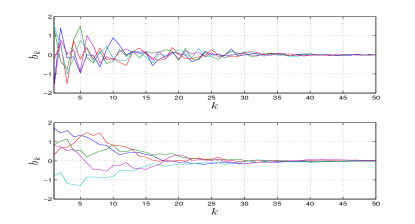
Figure 1: Top panel. Five realizations of $\mathbf{b}$ using the Diagonal kernel. Bottom panel. Five realizations of $\mathbf{b}$ using the Tuned-Correlated kernel.

As we see, in all these realizations $b_{k}$ decays in an exponential way. Indeed, for any realization of $\mathbf{b}$ we have that $\|\mathbf{b}\|^{2}_{K^{-1}}<\infty$ almost surely which implies that $b_{k}$ decays in an exponential way almost surely.

Proposition 1

Let $\hat{\mathbf{b}}_{ML}$ be the estimate using $K_{DI}$. If the corresponding polynomial $\hat{b}_{ML}(z)$ is nonnull, then it has zeros inside the unit circle.

Proof:

By (III) we have that

$$(\hat{\Sigma}+R)\hat{\mathbf{b}}_{ML}=\tilde{b}_{0}^{-1}v$$ (27)

where

$$R=((N-n)\lambda K)^{-1}:=\mathrm{diag}(r_{1},r_{2}\ldots r_{n+1})$$ (28)

and $r_{k}=((N-n)\lambda\beta^{k})^{-1}$. Thus, $r_{k+1}\geq r_{k}>0$. Let $\breve{z}$ be a zero of $\hat{b}_{ML}(z)$. If $\breve{z}=0$, then it is inside the unit circle and we have finished. Otherwise we have $\breve{z}\neq 0$. Define

$$u_{k}=\left\{\begin{array}[]{ll}\hat{b}_{0},&k=1\\ \breve{z}u_{k-1}+\hat{b}_{k-1},&k=2\ldots n\\ \end{array}\right.$$ (31)

where $\hat{\mathbf{b}}_{ML}=[\,\hat{b}_{0}\;\hat{b}_{1}\ldots\,\hat{b}_{n}\,]^{T}$. Accordingly,

$$u=\breve{z}\tilde{u}+\hat{\mathbf{b}}_{ML}$$ (32)

where $u=[\,u_{1}\;u_{2}\ldots\,u_{n}\;0\,]^{T}$ and $\tilde{u}=[\,0\;u_{1}\;u_{2}\ldots\,u_{n}\,]^{T}$. Using (32), we have

$$u^{*} (\hat{\Sigma}+R)u=(\overline{\breve{z}}\tilde{u}^{*}+\hat{\mathbf{b}}_{ML}^{T})(\hat{\Sigma}+R)(\breve{z}\tilde{u}+\hat{\mathbf{b}}_{ML})$$

$$=|\breve{z}|^{2}\tilde{u}^{*}(\hat{\Sigma}+R)\tilde{u}+\hat{\mathbf{b}}_{ML}^{T}(\hat{\Sigma}+R)\hat{\mathbf{b}}_{ML}+2\Re[\breve{z}\hat{\mathbf{b}}_{ML}^{T}(\hat{\Sigma}+R)\tilde{u}]$$

$$=|\breve{z}|^{2}\tilde{u}^{*}(\hat{\Sigma}+R)\tilde{u}+\hat{\mathbf{b}}_{ML}^{T}(\hat{\Sigma}+R)\hat{\mathbf{b}}_{ML}+2\tilde{b}_{0}^{-1}\Re[\breve{z}v^{T}\tilde{u}]$$ (33)

where in the last equality we exploited (27). Notice that $v^{T}\tilde{u}=0$, accordingly the last term on the right hand side is equal to zero. Moreover $u^{*}\hat{\Sigma}u=\tilde{u}^{*}\hat{\Sigma}\tilde{u}$ because $\hat{\Sigma}$ is a Toeplitz matrix. Therefore,

$$u^{*} (\hat{\Sigma}+R)u=|\breve{z}|^{2}u^{*}\hat{\Sigma}u+|\breve{z}|^{2}\tilde{u}^{*}R\tilde{u}+\hat{\mathbf{b}}_{ML}^{T}(\hat{\Sigma}+R)\hat{\mathbf{b}}_{ML}.$$ (34)

Finally notice that

$$\tilde{u}^{*}R\tilde{u}=\sum_{k=1}^{n}r_{k+1}|u_{k}|^{2}\geq\sum_{k=1}^{n}r_{k}|u_{k}|^{2}=u^{*}Ru.$$ (35)

Using the latter inequality in (34), we obtain

$$u^{*} (\hat{\Sigma}+R)u\geq|\breve{z}|^{2}u^{*}(\hat{\Sigma}+R)u+\hat{\mathbf{b}}_{ML}^{T}(\hat{\Sigma}+R)\hat{\mathbf{b}}_{ML}$$ (36)

and thus

$$(1-|\breve{z}|^{2})u^{*} (\hat{\Sigma}+R)u\geq\hat{\mathbf{b}}_{ML}^{T}(\hat{\Sigma}+R)\hat{\mathbf{b}}_{ML}.$$ (37)

The right hand side in (37) is positive because $\hat{\Sigma}+R>0$ and $\hat{\mathbf{b}}_{ML}\neq 0$ (otherwise $\hat{b}_{ML}(z)=0$). Moreover, $u^{*}(\hat{\Sigma}+R)u>0$ because $u\neq 0$ (otherwise $\hat{\mathbf{b}}_{ML}=0$). Accordingly, we have $1-|\breve{z}|^{2}>0$, that is $\breve{z}$ is inside the unit circle. ∎

It is worth noting the proof above is in the same spirit of the one in [1165162] for the Yule-Walker equations in (14).

III-B Tuned-Correlated (TC) kernel

We consider the kernel matrix $K_{TC}$ whose entry in position $(t,s)$ is defined as

$$[K_{TC}]_{ts}=\beta^{\max(t,s)}-\beta^{n+2},\;\;t,s=1\ldots n+1$$ (38)

where $\beta\in(0,1)$. It is worth noting that $K_{TC}$ in (38) is a modified version of the one proposed in [chen2012estimation]. Indeed, the latter is defined as

$$[\tilde{K}_{TC}]_{t,s}=\beta^{max(t,s)},\;\;t,s=1\ldots n+1.$$ (39)

However, for $n$ large the two kernel matrices $\tilde{K}_{TC}$ and $K_{TC}$ are very similar. In Figure 1 (bottom panel) we show five realizations of $\mathbf{b}\sim\mathcal{N}(0,\lambda K_{DI})$ with $\lambda=1$ and $\beta=0.85$. As we see, in all these realizations $b_{k}$ decays in an exponential way. Moreover, these impulse responses are more smooth than the ones using the diagonal kernel. Also in this case, for any realization of $\mathbf{b}$ we have that $b_{k}$ decays in an exponential way almost surely. It is not difficult to prove that

$$K_{TC}=(FDF^{T})^{-1}$$ (40)

where

$$F =\left[\begin{array}[]{ccccc}1&0&\ldots&\ldots&0\\ -1&1&\ddots&&\vdots\\ 0&\ddots&\ddots&&\vdots\\ \vdots&\ldots&&&\vdots\\ 0&\ldots&\ldots&-1&1\end{array}\right]$$ (46)

$$D =\frac{1}{\beta-\beta^{2}}\mathrm{diag}\left(1,\frac{1}{\beta},\frac{1}{\beta^{2}}\ldots\,\frac{1}{\beta^{n-1}},\frac{1}{\beta^{n}}\right).$$ (47)

Proposition 2

Let $\hat{\mathbf{b}}_{ML}$ be the estimate using $K_{TC}$. If the corresponding polynomial $\hat{b}_{ML}(z)$ is nonnull, then it has zeros inside the unit circle.