Science with the TianQin observatory: Preliminary results on stellar-mass binary black holes

Abstract

We study the prospect of using TianQin to detect stellar-mass binary black holes (SBBHs). We estimate the expected detection number as well as the precision of parameter estimation on SBBH inspirals, using five different population models. We note TianQin can possibly detect a few SBBH inspirals with signal to noise ratios greater than 12; lowering the threshold and combining multiple detectors can both boost the detection number. The source parameters can be recovered with good precision for most events above the detection threshold. For example, the precision of the merger time most likely occurs near 1s, making it possible to guide the detection of the ground-based detectors, the precision of the eccentricity $e_{0}$ most likely occurs near $10^{-4}$, making it possible to distinguish the formation channels, and the precision of the mass parameter is better than $10^{-6}$ in general and most likely occurs near $10^{-7}$. We note, in particular, that for a typical merger event, the error volume is likely to be small enough to contain only the host galaxy, which could greatly help in the study of gravitational wave cosmology and relevant studies through the multimessenger observation.

I Introduction

The gravitational collapse of massive stars can produce stellar-mass black holes with a mass range from a few to one hundred solar masses Burrows (1988); O’Connor and Ott (2011); Colpi and Sesana (2017). Other mechanism can also produce black holes with similar masses, for example, primordial black holes may result from the discontinuity or unevenness of matter distribution in the very early universe, and the PBHs channel for the formation of SBHs cannot yet be fully excluded by observations Bird et al. (2016); Carr et al. (2016); Sasaki et al. (2016); Ali-Haïmoud et al. (2017); Inomata et al. (2017); Ando et al. (2018); Chen and Huang (2018); Sasaki et al. (2018).

Before the first gravitational wave (GW) detection of stellar-mass binary black holes coalescence by the LIGO Scientific Collaboration and Virgo Collaboration (LVC) Abbott et al. (2016a), SBHs can only be observed by effects induced on their companions as well as through their accretion process with the electromagnetic (EM) observations. More specifically, with the EM channel, our understanding about SBHs came mostly from the investigations of x-ray binary (XRB), which consists of a stellar object and an accreting compact object. At present, 22 XRBs containing SBHs have been observed Abbott et al. (2016b), with most of the SBHs in these systems being lighter than $20M_{\odot}$. SBHs with higher masses have been claimed for detection, but mainly they remain under debate Liu et al. (2019). Observations of SBHs in EM channels indicated that there might be a gap between the most massive neutron stars Freire et al. (2008); Özel and Freire (2016); Margalit and Metzger (2017) and the lightest black holes with mass at about $5M_{\odot}$ Ozel et al. (2010); Farr et al. (2011); Kreidberg et al. (2012). It was proposed that the existence of this gap could be constrainted by GW observation Littenberg et al. (2015); Mandel et al. (2015, 2017); Kovetz et al. (2017)( cf. in the third observational run (O3) LVC reported possible observations of compact objects in this mass gap LIGO and scientific collaboration (2019a, b, c)). Before the GW detection, there were large uncertainties on the merger rates of SBBHs, ranging from $0.1$ to $\sim 300{\rm Gpc^{-3}yr^{-1}}$ Abadie et al. (2010); Downing et al. (2010, 2011); Mennekens and Vanbeveren (2014); Dominik et al. (2015); Rodriguez et al. (2015); Mandel and de Mink (2016).

The understanding of SBHs was revolutionized on September, 14^th, 2015, when the first GW signal from the merging stellar-mass binary black hole (BBH), later named as GW150914, was detected by the advanced LIGO (aLIGO) detectorsAbbott et al. (2016a, a, b, c, d, e, f, g, h, 2017a, i, j). A new window of GW has been opened to observe the Universe since. Further analysis reveals that the component masses of GW150914 are $35.6^{+4.8}_{-3.0}M_{\odot}$ and $30.6^{+3.0}_{-4.4}M_{\odot}$ respectively, with a redshift of $z=0.09^{+0.03}_{-0.03}$ Abbott et al. (2019a). The event, followed by nine other announced detections of SBBHs mergers and one announced detection of binary neutron star (BNS) merger by aLIGO and Virgo in the the first observational run (O1) and the second observational run (O2), marked the beginning of GW astronomy Abbott et al. (2016k, l, k, 2017b, 2017c, 2017d, 2017e, 2017f, 2017g, 2017h). In the O3, LVC published the detections of GW190412 and GW190425 Abbott et al. (2020a, b), and a list of compact binary coalescence alerts were released to public promptly. A more in-depth analysis is yet to be published. In the future, more detectors, like KAGRA Aso et al. (2013), are also aiming to join the collaboration and contribution.

The component masses of many SBHs observed by LVC are greater than $20M_{\odot}$, which is systematically larger than those in XRBs Abbott et al. (2019a, b). Meanwhile, the direct observation of BBH mergers greatly improve our understanding on their event rates. The observation of GW150914 alone constraints the rate to be $2-400{\rm Gpc^{-3}yr^{-1}}$ Abbott et al. (2016), while combining all events detected in O1 and O2 further shrinks the range to $25-109{\rm Gpc^{-3}yr^{-1}}$ Abbott et al. (2019b). All observed individual black holes masses are consistent with the theoretical upper limit of $\sim 50M_{\odot}$ induced by the pulsational pair-instability supernova (PPISN) and pair-instability supernova Heger and Woosley (2002); Belczynski et al. (2016); Woosley (2017); Spera and Mapelli (2017); Marchant et al. (2019).

The observation of SBBHs mergers poses two questions: how do SBHs form and how do they bind into binaries. SBHs may originate from three scenarios: (i) The collapse of massive stars, which depends strongly on the star’s metallicity, stellar rotation, and the microphysics of stellar evolution, which metallicity has the greatest impact. Lower metallicities lead to weaker stellar winds and can result in the formation of more massive SBHs Belczynski et al. (2010a); Mapelli et al. (2013); Spera et al. (2015). (ii) SBHs from PBHs Bird et al. (2016); Clesse and García-Bellido (2017); Sasaki et al. (2016); Kashlinsky (2016); Sasaki et al. (2018). PBHs can be formed through several mechanisms, the most popular being the gravitational collapse of overdensity regions Niemeyer and Jedamzik (1998); Shibata and Sasaki (1999); Musco et al. (2005); Polnarev and Musco (2007); Musco et al. (2009); Nakama et al. (2014); Harada et al. (2013). As the mass spectrum for this process can be quite wide, there will be no difficulty for massive SBHs formed through this channel Garcia-Bellido and Ruiz Morales (2017); Sasaki et al. (2018). (iii) SBHs could also be a product of former SBBH mergers O’Leary et al. (2016); Fishbach and Holz (2017); Gerosa and Berti (2017); Rodriguez et al. (2018); Veske et al. (2020) .

On the other hand, the binding of SBBHs can be largely categorized into two channels, where great progress has been made since the first GW detection, which is also reflected from the update of esitmated rates. (i) Coevolution of massive star binaries (e.g., (Vanbeveren, 2009; Belczynski et al., 2010b; Abbott et al., 2016b; Kruckow et al., 2018; Giacobbo and Mapelli, 2018)), with the corresponding merger rates ranging from $6$ to $240{\rm Gpc^{-3}yr^{-1}}$ (e.g., (Mapelli and Giacobbo, 2018; Buisson et al., 2020)). In this scenario, SBBHs will inherit the orbits and spins of their stellar progenitors; frictions within common envelope and other late stellar evolution process will shrink the eccentricities and align component of SBH spin to the orbital angular momentum. (ii) Dynamical process in dense stellar environments (e.g., (Portegies Zwart and McMillan, 2000; Gultekin et al., 2004, 2006; Abbott et al., 2016b; Chatterjee et al., 2017; Zevin et al., 2019; Tagawa et al., 2019; Samsing et al., 2019)), with a meger rate estimation within the range of $5-70{\rm Gpc^{-3}yr^{-1}}$ (e.g., (Rodriguez et al., 2016a, b; Park et al., 2017; Kumamoto et al., 2020)). The dynamical nature of their origin would implicate a relatively large orbital eccentricities as well as an isotropic distribution of the spins for the component SBHs Samsing et al. (2014); Antonini et al. (2016); Abbott et al. (2019b); Samsing and D’Orazio (2018); Kremer et al. (2019). Moreover, if SBBHs are composed of PBHs, then they are also expected to be formed through the dynamical encounter process Sasaki et al. (2016); Bird et al. (2016); the merger rates depend on the fraction of PBHs in dark matter and mass function (e.g., (Raidal et al., 2017; Chen and Huang, 2018; Raidal et al., 2019)). These SBBHs are also expected to have large orbital eccentricities Cholis et al. (2016).

While SBBHs merge at high frequencies where ground-based GW detectors are most sensitive, GW signals from their early inspiral could be observed by space-borne GW detectors with sensitive frequencies at millihertz range. By adopting a nominal detection threshold of signal-to-noise ratio (SNR) equal to 8, several studies claim that eLISA/LISA could individually resolve up to thousands of SBBHs Sesana (2016, 2017); Seto (2016); Kyutoku and Seto (2016), and the detection capability of Pre-DECIGO (recently renamed as B-DECIGO) has also been investigated Nakamura et al. (2016); Isoyama et al. (2018). New proposals for future generation space-borne GW detectors have also been proposed to better observe the SBBHs Sedda et al. (2019); Kuns et al. (2019).

With the expected SBBHs detections from space-borne GW detectors, a number of studies have explored their potential to distinguish the formation scenarios of SBBHs, by measuring the orbital eccentricities Nishizawa et al. (2016, 2017); Breivik et al. (2016), by using imprint of center of mass acceleration of SBBHs on the GW signals Inayoshi et al. (2017); Randall and Xianyu (2019), and by counting the detection rates Gerosa et al. (2019); Randall and Xianyu (2019). Furthermore, if the host galaxy of the SBBHs can be successfully identified, such systems could also provide a powerful laboratory for cosmology and fundamental physics. It is argued that SBBHs detections in millihertz band could be used to study cosmology as standard sirens Del Pozzo et al. (2018a). Reference Kyutoku and Seto (2017) proposes that LISA can use SBBHs detections to measure the Hubble parameter. Space-borne detectors could also constrain certain parameters of modified gravity theories with great precisions Barausse et al. (2016); Chamberlain and Yunes (2017).

Multiband GW astronomy is an important aspect of the science with SBBHs Sesana (2016); Seto (2016). The joint observation of space-borne and ground-based GW detectors could increase the scientific payoff, such as improving the constraint on the source parameters of SBBHs or on the consistency tests of general relativity Vitale (2016); Tso et al. (2019) and lowering the detection SNR threshold for space-based detectors by using information from ground-based detectors Wong et al. (2018).

The space-based GW observatory TianQin is expected to start operation around 2035 Luo et al. (2016). In this paper, we focus our attention on the detection ability as well as the precision of parameter estimation of TianQin on SBBHs. A collection of five different SBBHs mass distributions, with corresponding rates inferred from GW observations, is adopted. Based on the detection number as well as parameter estimation calculations, we further investigate the capability of TianQin to provide an early warning, and to explore its potential to multiband GW observations and multimessenger studies. We also discuss the potential of TianQin on astrophysics and fundamental physics with SBBHs, such as discriminating the formation channels of SBBHs, etc.

The paper is organised as follows. In Sec. II, we introduce the SBBH mass distribution models that we need in the study. In Sec. III, we describe the waveform and the statistical method employed. In Sec. IV, we present the main results of this work. In Sec. V, we conclude with a short summary. Throughout the paper, we use the geometrical units ($G=c=1$) unless otherwise stated.

II Mass distribution models

Prior to the GW detections of SBBH mergers, their mass distribution was derived by studying the evolution of massive stars. Observational evidence indicates that the initial mass function (IMF) for progenitors is well approximated by a single power law Salpeter (1955); the power-law model thus adopts the extreme assumptions that the mass distribution of SBHs follows closely with the IMF, while the other extreme model assumes a flat-in-log distribution. These two extreme models were adopted for relevant calculations Dominik et al. (2012); Fryer and Kalogera (2001); Fryer et al. (2012); Spera et al. (2015). During the calculation of merger rate, the selection bias makes the flat-in-log model a pessimistic prediction while the power law an optimistic model in terms of the SBBHs merger rate Dominik et al. (2012); Fryer and Kalogera (2001); Fryer et al. (2012); Spera et al. (2015). As GW observation results accumulate, several phenomenological mass distribution models of SBBHs are constructed and calibrated: models A, B, and C Abbott et al. (2019b), taking into consideration the SBH mass gaps Fishbach and Holz (2017) and an excess of SBHs with masses near $40M_{\odot}$ caused by PPISN Talbot and Thrane (2018). More details of the five models can be found in Appendix appendix a: mass distribution model. For the five models, the distributions of primary mass $m_{1}$ and the mass ratio $q$ are shown in Fig. 1. The obvious outlier is the flat-in-log model, showing a much steeper tail in heavier end.

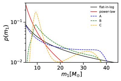
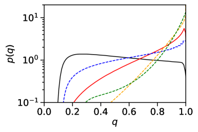
Figure 1: Distribution of the primary mass $m_{1}$ (left) and the mass ratio $q$ (right) for five mass models. The black and red solid lines represent models flat-in-log and power law; blue, green, and orange dashed lines denote models A, B, and C, respectively.

Previously, the merger rate of SBBHs $\mathcal{R}$ was mostly obtained through population synthesis, and it span 3 orders of magnitude Abadie et al. (2010). With the GW detection of SBBHs by LVC, by correcting the selection bias introduced by the assumed underlying mass distribution models, one can derive the corresponding merger rates. Currently the uncertainty of merger rate has been greatly reduced Abbott et al. (2016, 2019a, 2019b). The merger rate distributions in comoving volume of the five mass distribution models are listed in Table 1 in Appendix appendix a: mass distribution model and plotted in Fig. 2, respectively. All distributions roughly follow the log-normal distributions. We note that since the flat-in-log model assumes a much shallower tail than the remaining four models, combined with the selection bias of ground-based GW detectors toward higher mass SBBH mergers, the same amount of detections would translate into lower overall rates.

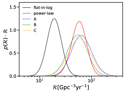
Figure 2: The distributions of merger rates $\mathcal{R}$ of the five mass models. The black and red solid lines represent models flat-in-log and power law; blue, green, and orange dashed lines denote models A, B, and C, respectively.

III Method

III.1 Waveform and response

Since in the mHz range where the space-borne GW detectors are most sensitive to, SBBHs locate well within the inspiral stage; thus, post-Newtonian (PN) waveform is sufficient to precisely describe the waveform Mangiagli et al. (2019). For a circular orbit SBBH system consisting of two SBHs with masses $m_{1}$ and $m_{2}$, the emitted inspiral GW in the detector frame can be described as Colpi and Sesana (2017)

$$h_{+}(t) =\frac{2\mathcal{M}^{5/3}(\pi f)^{2/3}(1+\cos^{2}\iota)}{d}\cos\left(\int{\rm d}t\,2\pi f\right),$$ (1a)

$$h_{\times}(t) =-\frac{4\mathcal{M}^{5/3}(\pi f)^{2/3}\cos\iota}{d}\sin\left(\int{\rm d}t\,2\pi f\right),$$ (1b)

where $f$ is the frequency of GW, $d$ is the distance between the detector and the SBBH, $\mathcal{M}=\eta^{3/5}M$ ($\eta=m_{1}m_{2}/M^{2}$ being the symmetric mass ratio and $M=m_{1}+m_{2}$ being the total mass) is the chirp mass, and $\iota=\arccos(\hat{\mathbf{n}}\cdot\hat{\mathbf{L}})$ is the inclination angle of the orbit to the line of sight. Notice that the redshift $z$ will modify the frequency/time by a factor of $1+z$. In practice, we replace distance $d$ with the luminosity distance $D_{L}$. Also, the chirp mass and total mass will be converted to the redshifted quantities in the observer frame Colpi and Sesana (2017),

$$\{\mathcal{M},M\}\rightarrow\{\mathcal{M}(1+z),M(1+z)\}.$$ (2)

Throughout the paper, relevant mass parameters are referred to the redshifted quantities.

The TianQin satellites are designed to follow a geocentric orbit, with arm length of about $L=\sqrt{3}\times 10^{5}$ km, performing laser interferometry to detect GW signals. The orientation of the orbital plane is fixed in space. To cope with the converse effect of the sunlight, the initial design of TianQin opts for a conservative strategy by observing only for every other three months. The three arms of the TianQin detector can be combined into two independent Michelson interferometers in the low frequency region ($f<f_{\ast}\equiv 1/(2\pi L)\approx 0.28{\rm Hz}$), which is generally valid for most of the SBBHs Hu et al. (2019, 2017).

For each Michelson interferometer, the detected signal $h(t)$ can be expressed as Klein et al. (2016)

$$h_{\alpha}(t) =\frac{\sqrt{3}}{2}\left[F^{+}_{\alpha}(t)h_{+}(t-t_{D})+F^{\times}_{\alpha}(t)h_{\times}(t-t_{D})\right],\qquad\alpha=1,2$$ (3)

$$t_{D} =R\sin\bar{\theta}_{S}\cos[\bar{\Phi}(t)-\bar{\phi}_{S}]\,,$$ (4)

where $t_{D}$ is the delay time between the interferometer and the solar system barycenter (SSB), $R=1$ AU and $\bar{\Phi}(t)=\bar{\phi}_{0}+2\pi t/T$, $T=1$ year is Earth’s orbital period around the Sun, and $\bar{\phi}_{0}$ is the initial location of TianQin at time $t=0$. Note the barred variables are quantities in the frame fixed on SSB and the unbarred variables are quantities in the detector frame. In the low frequency region, the antenna pattern functions $F_{\alpha}^{+,\times}(t)$ are Cutler (1998)

$$F_{1}^{+}(t) =\frac{1}{2}(1+\cos^{2}\theta_{S})\cos 2\phi_{S}\cos 2\psi_{S}-\cos\theta_{S}\sin 2\phi_{S}\sin 2\psi_{S},$$ (5a)

$$F_{1}^{\times}(t) =\frac{1}{2}(1+\cos^{2}\theta_{S})\cos 2\phi_{S}\sin 2\psi_{S}+\cos\theta_{S}\sin 2\phi_{S}\cos 2\psi_{S},$$ (5b)

$$F_{2}^{+}(t) =F_{1}^{+}(\theta_{S},\phi_{S}-\frac{\pi}{4},\psi_{S}),$$ (5c)

$$F_{2}^{\times}(t) =F_{1}^{\times}(\theta_{S},\phi_{S}-\frac{\pi}{4},\psi_{S}),$$ (5d)

where $\theta_{S}$ and $\phi_{S}$ are the altitude and azimuth angle, respectively, of the source. The polarization angle $\psi_{S}$ is defined as

$$\tan\psi_{S}=\frac{\mathbf{\hat{L}}\cdot\mathbf{\hat{z}}-(\mathbf{\hat{L}}\cdot\mathbf{\hat{n}})(\mathbf{\hat{z}}\cdot{\mathbf{\hat{n}}})}{\mathbf{\hat{n}}\cdot(\mathbf{\hat{L}}\times\mathbf{\hat{z}})},$$ (6)

where $\mathbf{\hat{z}}$ is the unit normal vector of the orbital plane of TianQin, $\mathbf{\hat{n}}$ is the unit vector to the source, and $\mathbf{\hat{L}}$ is the unit vector of the angular momentum of the source. Since we ignore the impact of BH spins, the polarization angle $\psi_{S}$ is fixed.

Away from the low frequency region, i.e. for $f>f_{\ast}$, the antenna pattern functions are frequency dependent and they are also complicated to calculate. In this study, we adopt a common simplification by absorbing such frequency dependence into the detector noise and use (5) for the whole frequency range targeted by TianQin.

As we will see in Sec. III.2, it is convenient to perform calculation in the frequency domain. We express the frequency domain signal $\widetilde{h}_{\alpha}(f)$ as the Fourier transform of the time domain signal

$$\widetilde{h}_{\alpha}(f)=\frac{\sqrt{3}}{2}\left\{\mathcal{F}[h_{+}(t-t_{D})F_{\alpha}^{+}(t)]+\mathcal{F}[h_{\times}(t-t_{D})F_{\alpha}^{\times}(t)]\right\},$$ (7)

with

$$\mathcal{F}[h_{+}(t-t_{D})F^{+}_{1}(t)] =\frac{1}{4}(1+\cos^{2}\theta_{S})\left[e^{2i\zeta_{1}(f-2f_{0})}\widetilde{h}_{+}(f-2f_{0})+e^{-2i\zeta_{2}(f+2f_{0})}\widetilde{h}_{+}(f+2f_{0})\right]\cos 2\psi_{S}$$

$$-\frac{i}{2}\cos\theta_{S}\left[-e^{2i\zeta_{1}(f-2f_{0})}\widetilde{h}_{+}(f-2f_{0})+e^{-2i\zeta_{2}(f+2f_{0})}\widetilde{h}_{+}(f+2f_{0})\right]\sin 2\psi_{S},$$ (8a)

$$\mathcal{F}[h_{\times}(t-t_{D})F^{\times}_{1}(t)] =\frac{1}{4}(1+\cos^{2}\theta_{S})\left[e^{2i\zeta_{1}(f-2f_{0})}\widetilde{h}_{\times}(f-2f_{0})+e^{-2i\zeta_{2}(f+2f_{0})}\widetilde{h}_{\times}(f+2f_{0})\right]\sin 2\psi_{S}$$

$$+\frac{i}{2}\cos\theta_{S}\left[-e^{2i\zeta_{1}(f-2f_{0})}\widetilde{h}_{\times}(f-2f_{0})+e^{-2i\zeta_{2}(f+2f_{0})}\widetilde{h}_{\times}(f+2f_{0})\right]\cos 2\psi_{S},$$ (8b)

$$\mathcal{F}[h_{+}(t-t_{D})F^{+}_{2}(t)] =\mathcal{F}[h_{+}(t-t_{D})F^{+}_{1}(\phi_{S0}-\frac{\pi}{4})],$$ (8c)

$$\mathcal{F}[h_{\times}(t-t_{D})F^{\times}_{2}(t)] =\mathcal{F}[h_{\times}(t-t_{D})F^{\times}_{1}(\phi_{S0}-\frac{\pi}{4})],$$ (8d)

where $\mathcal{F}[\dots]$ denotes the Fourier transformation, $\zeta_{1}(f)=\phi_{S0}-\pi ft_{D}$, $\zeta_{2}(f)=\phi_{S0}+\pi ft_{D}$, $f_{0}\approx 3.176\times 10^{-6}{\rm Hz}$ is the orbital frequency of the TianQin satellites around the Earth, $\phi_{S0}$ is the initial location of sources, and $\widetilde{h}_{+,\times}(f)$ are Fourier transform of ${h}_{+,\times}(t)$. For more details, please refer to Appendix appendix b: Frequency response for a signal. We emphasize that although we assume a circular orbit in Eq. (1), Eqs. (5) are applicable to general orbits, such as the eccentricity is not zero.

For the post-Newtonian waveform, it has been suggested that a waveform up to 2PN order is sufficiently accurate for the precise measurement of SBBH with space-based GW detectors Mangiagli et al. (2019). Therefore, we adopt the restricted 3PN waveform with and eccentricity for $\widetilde{h}_{+,\times}(f)$ throughout our calculation Królak et al. (1995); Buonanno et al. (2009); Feng et al. (2019). The choice of a higher order PN waveform is to be conservative, especially considering the better sensitivity of TianQin in higher frequencies. We ignore the spin of SBBHs as the effect is expected to be minor in low frequencies Nishizawa et al. (2016).

III.2 Signal-to-noise ratio

The recorded data $s(t)$ contains two parts: the noise $n(t)$ and the GW signal $h(t)$,

$$s(t)=h(t)+n(t).$$ (9)

For the analysis of GW signal, it is convenient to define the inner product between two waveforms $h_{1}(t)$ and $h_{2}(t)$ Cutler and Flanagan (1994)

$$(h_{1}|h_{2})=4\Re\int_{0}^{+\infty}{\rm d}f\,\frac{\widetilde{h}_{1}^{\ast}(f)\widetilde{h}_{2}(f)}{S_{n}(f)},$$ (10)

where $\widetilde{h}_{1}(f)$ and $\widetilde{h}_{2}(f)$ are the Fourier transform of $h_{1}(t)$ and $h_{2}(t)$, respectively, and ^∗ represents complex conjugate, $S_{n}(f)$ is the power spectral density of detector noise $n(t)$. The pure noise for TianQin is characterized with

$$S_{N}(f)=\frac{1}{L^{2}}\left[\frac{4S_{a}}{(2\pi f)^{4}}\Big{(}1+\frac{10^{-4}{\rm Hz}}{f}\Big{)}+S_{x}\right],$$ (11)

with $S_{a}^{1/2}=1\times 10^{-15}\,{\rm m}\,{\rm s}^{-2}\,{\rm Hz}^{-1/2}$, $S_{x}^{1/2}=1\times 10^{-12}\,{\rm m}\,{\rm Hz}^{-1/2}$ Luo et al. (2016). However, in higher frequencies, when the low frequency approximation fails, the detector response to a given source falls rapidly. Therefore, we instead use the effective sensitivity curve $S_{n}$ for the inner product in the actual calculation,

$$S_{n}(f)=\frac{3}{20}\frac{S_{N}(f)}{\overline{R}(2\pi f)}$$ (12)

where $\overline{R}(2\pi f)$ is the averaged response function,

$$\overline{R}(2\pi f)=\frac{3}{20}\times\frac{g(2\pi f\tau)}{1+0.6(2\pi f\tau)^{2}}$$ (13)

where $\tau=L$ is the light travel time for a TianQin arm length, and the function $g(x)$ approaches unit for the lowest order approximation, with the higher order approximation listed in Wang et al. (2019).

For a given detector, the optimal SNR $\rho$ of a signal $h(t)$ is defined as the square root of inner product of $h$ with itself Cutler and Flanagan (1994)

$$\rho=(h|h)^{1/2}=\sqrt{4\Re\int_{0}^{+\infty}{\rm d}f\,\frac{\widetilde{h}^{\ast}(f)\widetilde{h}(f)}{S_{n}(f)}}.$$ (14)

If multiple detectors observe the same event simultaneously, then the overall SNR is defined as the root sum square of the individual SNR for the $k$th detector $\rho_{k}$,

$$\rho=\sqrt{\sum_{k}\rho_{k}^{2}}.$$ (15)

The nominal configuration of the TianQin constellation as proposed in Luo et al. (2016) follows a “3 months on+3 months off” observation pattern, causing gaps in the recorded data. As a result, the PN waveform has to be set zero for certain range of frequencies in (10). The frequency boundaries can be found from the instantaneous frequency at the time $t$ before the merger time $t_{c}$,

$$f=(5/256)^{3/8}\frac{1}{\pi}\mathcal{M}^{-5/8}(t_{c}-t)^{-3/8}\,,$$ (16)

where the leading order of PN expansion is used. In practice, with a given merger time $t_{c}$, we perform cutoff on frequencies when the detector is not operating using Eq. (16) and then apply Eq. (8) upon the truncated waveforms.

In this paper, we also consider the so-called twin constellation configuration of TianQin, which involves 2 three-satellite constellations perpendicular to each other while both being nearly perpendicular to the ecliptic plane. The twin constellations could alleviate the data gap issue of the one constellation configuration through the relay of observation.

III.3 Fisher information matrix

For a GW signal $h(t,\bm{\lambda})$, where the true physical parameter are $\bm{\lambda}$, the contamination of noise in the data means that it is probable that the maximum likelihood parameter $\hat{\bm{\lambda}}$ would be shifted from the true parameter by $\Delta\bm{\lambda}$: $\hat{\bm{\lambda}}=\bm{\lambda}+\Delta\bm{\lambda}$. The Fisher information matrix (FIM) is a useful tool to assess the covariance matrix associated with the maximum likelihood estimate Cutler and Flanagan (1994),

$$p(\Delta\bm{\lambda})\approx\sqrt{{\rm det}(\Gamma/2\pi)}\exp(-\frac{1}{2}\Gamma_{ij}\Delta\lambda^{i}\Delta\lambda^{j}),$$ (17)

where $\Gamma_{ij}$ is the FIM,

$$\Gamma_{ij}=\left(\frac{\partial h}{\partial\lambda^{i}}\middle|\frac{\partial h}{\partial\lambda^{j}}\right),$$ (18)

and the Cramer-Rao bound of the covariance matrix $\Sigma$ is given by the inverse of $\Gamma$, $\Sigma=\Gamma^{-1}$. For a network of detectors, the overall FIM is the summation over component FIMs,

$$\Gamma_{ij}=\sum_{k}\Gamma_{ij}^{k}.$$ (19)

Therefore, one can estimate the uncertainty as the square root of the corresponding diagonal component of $\Sigma$,

$$(\Delta\lambda^{i})_{{\rm rms}}=\sqrt{\Sigma_{ii}}\,.$$ (20)

One exception is the precision on the sky localization $\Delta\bar{\Omega}_{S}$, which can be obtained by Berti et al. (2005)

$$\Delta\bar{\Omega}_{S}=2\pi|\sin\bar{\theta}_{S}|(\Sigma_{\bar{\theta}_{S}\bar{\theta}_{S}}\Sigma_{\bar{\phi}_{S}\bar{\phi}_{S}}-\Sigma_{\bar{\theta}_{S}\bar{\phi}_{S}}^{2})^{1/2}.$$ (21)

Notice that FIM is only an approximation on the statistical uncertainty; thus, it cannot give an assessment on systematic uncertainty. Also, the approximation would generally fail in low SNR scenarios Vallisneri (2008); Rodriguez et al. (2013).

IV Results

IV.1 Detection number

We first study the expected detection number of SBBHs. For each mass model, we generate 200 Monte Carlo simulations for the corresponding merger catalogs. A preset detection threshold on SNR would then be applied to identify the detectable sources.

For each catalog, we first determine the number of merger events by randomly drawing from the merger rate distribution. Then, for each event, we randomize over all possible parameters, including the component masses, redshift, coalescence time, sky location and orbital angular momentum. We choose $\bar{\phi}_{S}$ and $\bar{\phi}_{L}$ to be uniform in the range $[0,2\pi]$, $\cos\bar{\theta}_{S}$ and $\cos\bar{\theta}_{L}$ to be uniform in the range $[-1,1]$, and the spatial distribution is chosen to be uniform in the comoving volume. We limit the distance of sources to $0<z<2$, and we use the standard $\Lambda{\rm CDM}$ cosmological model ($h=0.679,\Omega_{\Lambda}=0.694,\Omega_{M}=0.306$ Ade et al. (2016)). The coalescence time is evenly distributed in the comoving frame. The choice of the redshift upper limit is to be large enough so that the most optimal configuration would not exceed a preset threshold. As we will see in Fig. 4, binaries with larger $t_{c}$ have less possibility to be detected; therefore, we also set an upper limit on $t_{c}$ to a large enough value so that the possibility of detecting event with higher $t_{c}$ is negligible.

The detection threshold for SNR is chosen to be 5, 8, and 12. The choice of 5/8 is consistent with ground-based GW detection traditions and was widely used for a number of similar studies in the field Sesana (2016, 2017); Kyutoku and Seto (2016); Nakamura et al. (2016); Isoyama et al. (2018); Wong et al. (2018). By inhereting such threshold, we are allowed to make direct comparisons with relevant literatures. We stress, however, that the threshold 5 is quite optimistic and should only be meaningful when considering a network of GW detectors. It has been suggested in Moore et al. (2019) that a search using template bank would require an SNR threshold of $\sim 15$ for LISA detection, and the threshold could be reduced to $\sim 9$ through multidetector observation. We apply a similar procedure and calculate the expected SNR threshold to be $\sim 12$ for TianQin . Therefore, for the following calculation, we stick with the choice of 5, 8, and 12 on the SNR threshold.

In order to draw better informed conclusions on the capability of TianQin, we consider four different observation scenarios with the following combination or single detectors:

1. TQ for the TianQin constellation.

2. TQ I+II for the putative twin constellation configuration of TianQin.

3. TQ + LISA for the joint observation of TianQin and a LISA type detector (hereafter shorten as LISA).

4. TQ I+II + LISA for the joint observation of TianQin I+II and LISA.

We assume 5 years of operation time for TianQin, and 4 years for LISA, and we assume the same starting time for all detectors. Finally, we adopt Robson et al. (2019); Berti et al. (2005) for the LISA power spectral density and orbit.

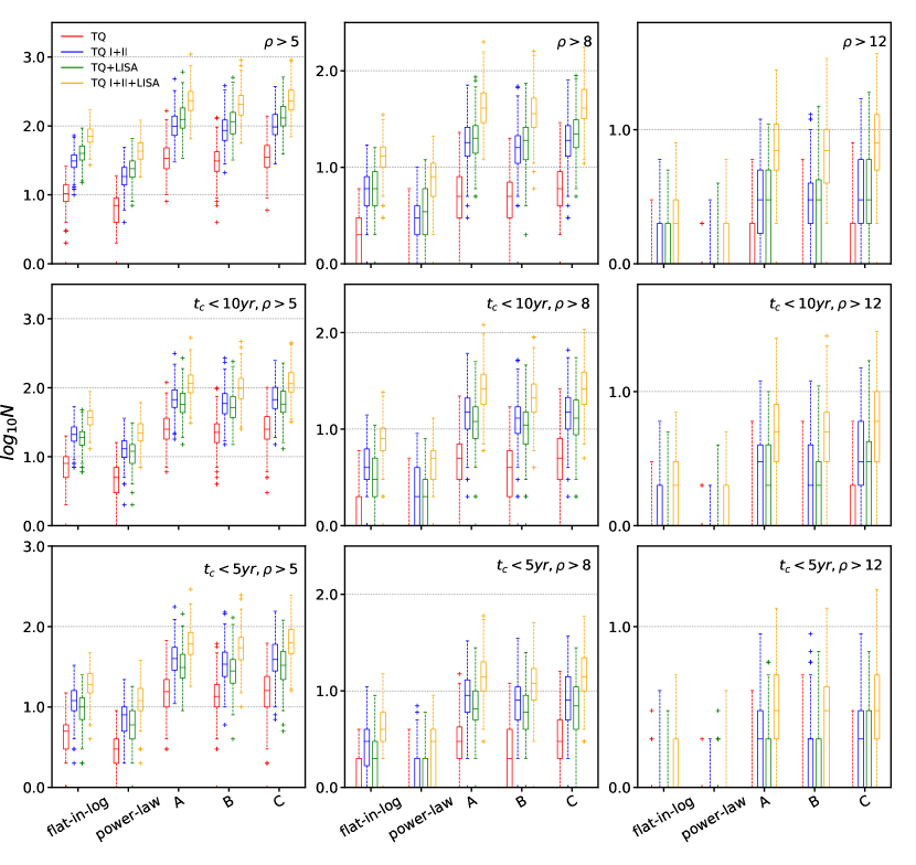
Figure 3: The box plots for detection number, under different mass distribution models (flat-in-log, power law, A, B, and C) and detector cases (TQ, TQ I+II, TQ+LISA, and TQ I+II + LISA). The left column setting $\rho_{\rm thr}=5$, the middle column $\rho_{\rm thr}=8$ and the right column $\rho_{\rm thr}=12$. The top panel shows number for all events, while the middle panel for events that will merge in 10 years after the operation of TianQin, and the bottom panel for 5 years.

The detection numbers over the whole mission lifetime for all detectors in all scenarios are shown as box plots in Fig. 3. For each case, a box plot illustrates the three quartiles with the middle line and the edges of the box; a whisker is used to indicate the extreme, or 1.5 times the box length when the furthest point is even further. The top, middle and bottom panels correspond to the expected detection numbers for all events, for events merged within 10 years, and for events merged within 5 years, respectively. The left, middle and right columns correspond to the detection threshold $\rho_{\rm thr}=5,8,$ and 12, respectively.

For the pessimistic scenarios, i.e., adopting a threshold of $\rho_{\rm thr}=12$, TianQin is expected to detect at most order 1 SBBH. With a network of detectors, like TQ I+II, TQ+LISA and TQ I+II+LISA, the detection number is expected to increase, and order 1 of such binaries would merge within 5$-$10 years. For the optimistic scenarios with $\rho_{\rm thr}=8$ for the detection threshold, adopting models A, B, and C for the mass models and considering all possible events, the expected detection number for TQ I+II, TQ+LISA, and TQ I+II+LISA could be a few dozens. For each case, the 90% credible interval spans 1 order of magnitude; for a given mass model, TQ I+II + LISA would have the most detections.

For a space-borne GW detector like TianQin, the detection rate from SBBHs is mostly affected by two factors, the overall merger rate and the normalized mass distribution. A more heavy-tailed SBBH distribution (with larger portion of more massive SBHs) produces louder events for TianQin, while a higher merger rate leads to more events, and so both can lead to a larger detection rate. We note that the mass distribution for the power-law model is significantly more heavy-headed (with larger portion of less massive SBHs) than all other models (Fig. 1), while the merger rate of flat-in-log model is significantly lower than all other models (Fig. 2). As a result, the flat-in-log and power law models expect comparable detection numbers, which are consistently lower than those from models A, B, and C.

By adding more detectors, naturally more detections are expected. This is reflected in Fig. 3 where green lines (TQ + LISA) and blue lines (TQ I+II) are always higher than red lines (TQ), while yellow lines (TQ I+II + LISA) are always the highest. We note TQ I+II and TQ+LISA have comparable detection numbers. This is caused by the fact that TianQin has both sensitivity in the high frequency region but less observation time compared to LISA.

By comparing the left and right columns in Fig. 3, one can see that a small difference in the SNR threshold can make a big difference in terms of the detection numbers. In the case $\rho_{\rm thr}=8$, almost all catalogs within all models predict a nonzero detection, with the most optimal cases predicting detection numbers to be reaching $\sim 100$. On the other hand, the case $\rho_{\rm thr}=12$ predicts much fewer detections. The fact that the detection number is quite sensitive to the choice of detection threshold is consistent with the result of Moore et al. (2019), where a threshold of $\rho_{\rm thr}\sim 15$ for LISA implies no detection at all. We remark that efficient detection algorithms are needed for relatively weak signals.

There is a difference between the detection numbers in the top, middle, and bottom panels, but they are of comparable orders, with those in the middle panel being about 60% of those in the top panel. As is obvious from Eq. (16), the instantaneous frequency is sensitive to the amount of time left before the final merger, and the frequency evolution is slower for those far away from the merger than those close to the merger. Limiting to sources that must merge within a certain amount of time will limit the frequency interval to be integrated in Eq. (14), hence leading to lower SNR and smaller detection numbers. Such fact indicates that for most mergers, a multiband GW observation can be expected to be performed within a short time.

IV.2 Parameters estimation

To study the precision of parameter estimation, we use the catalogs from the last subsection and focus on the test events that not only pass the detection threshold $\rho>8$ but also will merge within 5 years. We use the same 3PN waveform, but allowing a nonzero value of eccentricity $e_{0}$, which is defined as the instantaneous eccentricity for when GW frequency is 0.01Hz. Since most sources have a minimum frequency of about $10^{-3}$Hz, we expected their eccentricities to be smaller than 0.1 Nishizawa et al. (2016) due to GW circularization. We choose $e_{0}=0.01$ as a representative value Nishizawa et al. (2016).

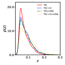
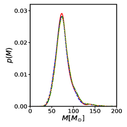
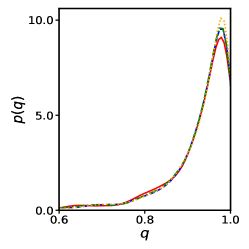
Figure 4: Parameters distributions for detectable events ($\rho>8$), assuming merge within 5 years (from left to right: redshift $z$, total mass $M$ and mass ratio $q$).

In Fig. 4, we present their distributions with respect to redshift $z$, total mass $M$ and symmetric mass ratio $\eta$. We notice that the difference between different mass models is very minor, and we show the result for model C as representatives. Since we distribute the events uniformly in comoving volume, the events follow a dependence on luminosity distance $p(D_{L})\propto D_{L}^{2}$, which is shown as rapidly rising below $z\sim 0.05$ in the redshift distribution. However, events with too far a distance would hardly pass the detection threshold. The two factors combined form a peak around $z\sim 0.05$ in the expected detected events. For a space-borne GW detector, all other factors being equal, a heavier SBBH always indicates a larger SNR. But the underlying distribution for SBH mass falls for larger masses. These two factors lead to a peak of $\sim 70M_{\odot}$ for total mass $M$. Finally, the mass ratio is heavily shifted toward unity; this is because the masses for SBHs have an upper limit, and an equally massive binary would form the heaviest binaries, meeting the preference of the detectors. We also note that different detector combinations would only change the redshift distribution, as more detectors means higher SNR, and the ability to detect more distant events.

We use the FIM method to study the precision on the parameter set $\bm{\lambda}=\{t_{c},\bar{\Omega}_{S},\ln\mathcal{M},\ln\eta,$ $\ln e_{0},\ln D_{L}\}$. Since the difference caused by different mass models is small, we still use model C as an example. The result is shown in Fig. 5. We notice that although the detection number differs quite a lot for different detector combinations, the normalized distribution for parameters is quite consistent for all parameters, and the spread of all parameter uncertainties are roughly about 1 order of magnitude, with those for the merger time and the luminosity distance being slightly narrower. This is mainly due to the fact that the uncertainty in parameter estimation is roughly proportional to the inverse of SNR, and applying a universal SNR threshold leads to the very similar distribution. More detectors mean larger numbers of high-SNR detections, but it does not necessarily mean high-SNR events have higher percentage. That being said, including LISA in the detector network does seem to help reduce the tail with $\Delta t_{c}$, i.e. the uncertainty in the estimation of the merger time.

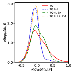
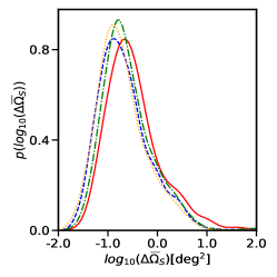
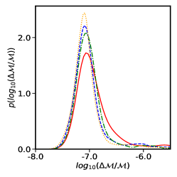
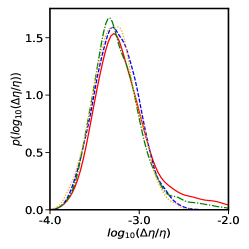
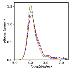
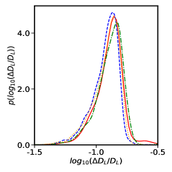
Figure 5: Estimation precision distributions of (a) coalescing time $t_{c}$, (b) sky localization $\bar{\Omega}_{S}$, (c) chirp mass $\mathcal{M}$, (d) symmetric mass ratio $\eta$ and (e) luminosity distance $D_{L}$. Red solid line, blue dashed line, green dash-dotted line, and orange dotted line represent TianQin, TianQin twin constellations, TianQin+LISA, and TianQin twin constellations+LISA, respectively.

The expected uncertainties for localization are remarkable. Using the most probable value from each plot as an indicator of TianQin’s capability to measure the corresponding parameter, one can see that TianQin can predict the merger time with a precision of $\Delta t_{c}\sim 1$s, and report the sky location as precise as $\Delta\bar{\Omega}_{S}\sim 0.1$ deg². This level of precision in space and time is good enough for EM telescopes as well as for ground-based GW observatories to prepare the examination toward the final merger moment.

Specifically, we remark the precise three-dimensional (3D) localization ability of TianQin, which is invaluable for multiband GW observation as well as multimessenger observations, as it can greatly help in the identification of the host galaxy, which could open a bright possibility on GW cosmology measurement. Combined with a $\Delta D_{L}/D_{L}\sim$ 20% relative error on luminosity distance, for a typical source located at redshift 0.05, the 3D error volume $\Delta V\sim D_{L}^{2}\Delta\bar{\Omega}_{s}\Delta D_{L}\sim$ 50Mpc³. For the loudest events, $\Delta V$ could be as small as $\sim 2{\rm Mpc^{3}}$. Note that when the detection threshold increases, $\Delta V$ of the worst localized events would be improved Del Pozzo et al. (2018b). For an average number density of Milky-Way-like galaxy of 0.01 Mpc^-3, this means that one could pinpoint the host galaxy for the event Abadie et al. (2010).

The mass parameters are among the most precise parameters to be measured. The chirp mass $\mathcal{M}$ has a huge effect on the phase of the PN waveform; a slight change in $\mathcal{M}$ could lead to a huge dephase. With a typical frequency of 0.01 Hz, and an observation duration of $\sim 10^{8}$s, an SBBH is expected to rotate $\sim 10^{6}$ cycles during the observation. Therefore, a relative error of $10^{-6}$ on frequency-related parameter can be expected, translating into a precise determination in the chirp mass relative error $\Delta\mathcal{M}/\mathcal{M}\sim 10^{-7}$. The phase evolution depends also on the symmetric mass ratio $\eta$, but only on higher order terms, so the precision is much lower than chirp mass, but still can reach a remarkable 0.1% relative error.

The eccentricity could also be very precisely determined, with the most probable relative uncertainty close to $\Delta e_{0}/e_{0}\sim 0.01\%$. So even if the eccentricity $e_{0}$ is as small as 0.01 at 0.01 Hz, TianQin can still precisely measure it and use it as a promising tool to help unveil the formation mechanisms of SBBHs.

To see how TianQin can join a network of detectors to improve on the precision of parameter estimation for future space-based GW missions, we use LISA as a reference mission and plot in Fig. 6 the distribution of the ratio $Q$ between the precision of parameter estimation with LISA alone and the precision of parameter estimation by two detector networks involving TianQin: TQ+LISA (green line) and TQ I+II + LISA (orange line). A larger value of $Q$ means a better improvement in precision. One can see that the precision of the coalescing time $t_{c}$, the sky localization $\bar{\Omega}_{S}$, the chirp mass $\mathcal{M}$, and symmetric mass ratio $\eta$ can all be significantly improved, and for some of them the improvement can be close to 1 order of magnitude. For parameters like the luminosity distance $D_{L}$, however, the improvement is less than 2, comparable to the improvement on the SNR. The reason is that the luminosity distance only affects the magnitude of GW, which is often measured with less accuracy than the GW phase.

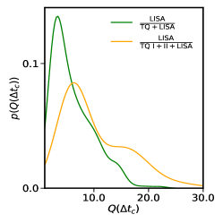
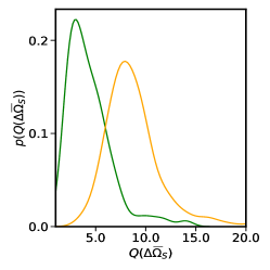
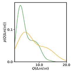
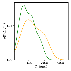
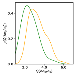
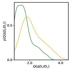
Figure 6: The improvement on the precision of parameter estimation of the (a) coalescing time $t_{c}$, (b) sky localization $\bar{\Omega}_{S}$, (c) chirp mass $\mathcal{M}$, (d) symmetric mass ratio $\eta$ and (e) eccentricity $e_{0}$, and (f) luminosity distance $D_{L}$, for TQ+LISA (green) and TQ I+II + LISA (brown), with LISA being the reference.

The orientation of the TianQin orbital plane is nearly fixed in space. We want to know how this feature will affect the precision of parameter estimation for sources located at different directions in space. For this purpose, we adopt a detector-based spherical coordinate system that uses the TianQin orbital plane as its equator. In this coordinate system, a celestial object would have a constantly changing azimuth, but a fixed altitude. We randomly choose $\phi_{S}$ and $\phi_{L}$ from the distribution $U(0,2\pi)$, $\cos\theta_{L}$ from the distribution $U(-1,1)$ and $t_{c}$ from $U(0,5)$ years for a group of SBBHs with $m_{1}=m_{2}=30M_{\odot}$ at $D_{L}$=200Mpc, and look at how the precision of parameter estimation varies with the altitude $\theta_{S}$. The result is shown in Fig. 7. One can see that precision for sources near the zenith and the nadir, corresponding to $\theta_{S}=0$ and $\theta_{S}=\pi$, is always better than that for sources near the equator, in the amount of about half to one decade. This is consistent with the general expectation that a GW detector has better sensitivity for sources near the zenith and nadir than for those near the equator. In the putative TianQin I+II network, a new constellation orthogonal to the initial TianQin constellation is introduced and the two constellations operate consecutively and repeatedly. We see in Fig. 7 that TianQin I+II has improved all sky response as expected.

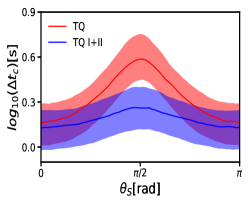
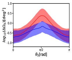
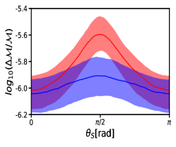
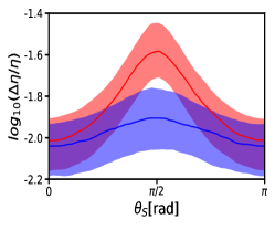
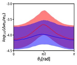
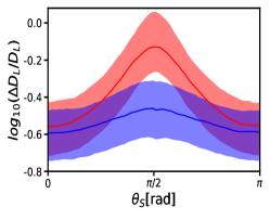
Figure 7: Parameter estimation precision dependence on altitude $\theta$ in the detector coordinate system, showing in (a) coalescing time $t_{c}$, (b) sky localization $\Omega_{S}$, (c) chirp mass $\mathcal{M}$, (d) symmetric mass ratio $\eta$, (e) eccentricity $e_{0}$, and (f) luminosity distance $D_{L}$. The line being the median while the shaded region reflects the central 50% credible interval.

The aforementioned calculations are all based on the method of FIM. As mentioned in Sec. III.3, it is expected that the validity of FIM will fade in low SNR cases. Therefore, we aim to investigate that to what extent can we trust the parameter estimation results from FIM. We follow Vallisneri to present the cumulative distribution for mismatch ratio $r$ over the isoprobability surface deduced from FIM method Vallisneri (2008). The mismatch ratio $r$ quantifies the difference from the exact value of likelihood and the derived value approximated by the FIM method. By adopting the mass parameter of GW150914, we present the cumulative distribution of logarithm of $r$ for different SNRs in Fig. 8. We notice that for events with an SNR of 8, for more than 90% of the randomly drawn points from the isoprobability surface, their actual likelihood deviates only slightly from the derived value, marking the validity of FIM in such SNR level. Furthermore, FIM conclusions can be largely trusted for events with SNRs as low as 4.

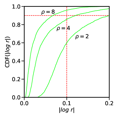
Figure 8: Cumulative distribution of logarithm of mismatch ratio $\log r$ for different SNRs, assuming the mass parameters of GW150914, to assess the validity of FIM. The curve of SNR 8 is higher than the 90% and $\log r=0.1$ point, meaning that the derived likelihood from FIM and the exact value are close enough and the results from FIM are trustworthy for SNR as low as 8.

V Summary

In this work, we carry out a systematic study on the capability of TianQin in terms of observing SBBH. We estimate the detection number of SBBHs as well as the precision of source parameter estimation with TianQin. In order to make the result as robust as possible, we use five models for the mass distribution and the corresponding merger rate of SBBH, i.e. the models flat-in-log, power law, A, B and C. In order to draw better informed conclusions on the capability of TianQin, we not only consider the detection capability of TianQin alone but also explore the detection capability of three detector networks containing TianQin: TQ I+II, TQ + LISA and TQ I+II + LISA.

We find that a network of multiple detectors is needed for the detection of SBBHs, for the pessimistic mass models (flat-in-log and power law) and the more strict SNR threshold, $\rho_{\rm thr}=12$. With the more optimistic mass models A, B and C, TianQin is expected to detect a few SBBHs. What’s more, if TianQin forms a detector network, such as TQ I+II, TQ + LISA and TQ I+II + LISA, the upper end of total expected detection number can reach over 10. When the SNR threshold is 8, the network of detectors is expected to detect $\sim 100$ at most.

Using the FIM method, we find that source parameters for the detected SBBHs events can be precisely determined. Using the most probable value from each plot in Fig. 5 as an indicator of TianQin’s capability to measure the corresponding parameter, we find that TianQin can measure the chirp mass to the order $10^{-7}$, measure the symmetric mass ratio $\eta$ better than the order $10^{-3}$, forecast the merger time $t_{c}$ with a precision of the order $\sim$1s, determine the sky location of the source with a precision of the order $\sim 0.1$ deg², determine the luminosity distance to $20\%$ level, and measure the eccentricity $e_{0}$ to the order $10^{-4}$. The high precision in the determination of the source parameters is of great importance for many scientific purposes. For example, a precise prediction for the final merger moment is important for the follow-up multimessenger observation using EM facilities and multiband GW observation with ground-based GW observatories; a high precision in the measurement of the eccentricity $e_{0}$ could help distinguish the formation channels of SBBHs and so on. A validity check for the FIM method is performed, and the corresponding conclusion is trustworthy for signals with an SNR as low as 8.

We highlight that the typical source localization error box has volume of the order $\Delta V\sim$ 50Mpc³, which is so small that it contains only one Milky-Way-like galaxy in average, and this could greatly help in the identification of the host galaxy and make possible a great deal of science Fan et al. (2014); Chassande-Mottin et al. (2011).

We note that if TianQin is operated within a network of detectors, such as TQ I+II, TQ + LISA, and TQ I+II + LISA, both the expected detection numbers and the precision of source parameter estimation can be significantly improved. This is true not only for TianQin but also for any other individual detector involved, such as LISA.

Compared to existing literature for similar space-based GW missions like LISA/eLISA Sesana (2016, 2017); Nishizawa et al. (2016); Tamanini et al. (2019)), our estimation of the detection number is smaller, but this is due less to the true difference between the detection capabilities of the detectors than to the mass models used in the study. In particular, we note larger high mass limits in the mass models have been used in earlier works, and this can significantly boost the expected detection numbers because space-borne GW detectors are more sensitive to heavier SBBHs. By adopting the same setup, the expected detection numbers can be as high as reported in previous studies with LISA.

In summary, TianQin can detect SBBH inspirals with good certainty and can measure the corresponding source parameters with impressive precisions. The analysis from TianQin data alone, as well as from multimessenger observation and multiband GW observation, promises great scientific return on astrophysics and fundamental physics related to SBBHs.

appendix a: mass distribution model

• Model flat-in-log

  The distribution of the masses of both SBBH components are independently flat on the logarithmic scale,
  

  $$p(m_{1},m_{2})\propto\frac{1}{m_{1}m_{2}},$$ (22)

  where $p(m_{1},m_{2})$ is the probability of SBBHs with component masses $m_{1}$ and $m_{2}$.

• Model power law

  The primary mass $m_{1}$ follows a power law distribution while the secondary mass $m_{2}$ follows a uniform distribution,

  $$p(m_{1},m_{2}) \propto\frac{m_{1}^{-\alpha}}{m_{1}-5M_{\odot}}\,,\quad\alpha=2.3\,.$$ (23)

In these two models, the component masses are bounded by $5M_{\odot}<m_{2}<m_{1}<50M_{\odot}$.

• Model A

  $$p(m_{1},m_{2}|\alpha,\beta_{q})\propto C(m_{1})m_{1}^{-\alpha}q^{\beta_{q}},$$ (24)

  where $5M_{\odot}\leqslant m_{2}\leqslant m_{1}\leqslant 41.6_{-4.3}^{+9.6}M_{\odot}$, $q=m_{2}/m_{1}$ is the mass ratio, $\alpha=0.4_{-1.9}^{+1.4}$ and $\beta_{q}=0$ are the power law index, and $C(m_{1})$ is a correction factor to make marginalized distribution of $m_{1}$ follow the power law with index of $\alpha$.

• Model B

  Model follows the same form as model A, but with $7.8_{-2.5}^{+1.2}M_{\odot}\leqslant m_{2}\leqslant m_{1}\leqslant 40.8_{-4.4}^{+11.8}M_{\odot}\,$ and $\alpha=1.3_{-1.7}^{+1.4},\beta_{q}=6.9_{-5.7}^{+4.6}\,$.

• Model C

  On top of Model B, the possible accumulation of SBH due to PPISN is characterized by a Gaussian component, and a smooth tail is included in the end, both making the model C more realistic,

  $$p(m_{1}|\theta) =\left[(1-\lambda_{m})A(\theta)m_{1}^{-\alpha}\Theta(m_{\rm max}-m_{1})+\lambda_{m}B(\theta)\exp\left(-\frac{(m_{1}-\mu_{m})^{2}}{2\sigma_{m}^{2}}\right)\right]$$

  $$\times S(m_{1},m_{\rm min},\delta m)$$ (25)

  $$p(q|m_{1},\theta) =C(m_{1},\theta)q^{\beta_{q}}S(m_{2},m_{\rm min},\delta m)$$ (26)

  Here $\theta=\{\alpha,m_{\rm max},m_{\rm min},\beta_{q},\lambda_{m},\mu_{m},\sigma_{m},\delta m\}$, whereas $\mu_{m}=29.8_{-7.3}^{+5.8}M_{\odot}$ and $\sigma_{m}=6.4_{-4.2}^{+3.2}M_{\odot}$ describe the mean and standard deviation of the Gaussian component; $\lambda_{m}=0.3^{+0.4}_{-0.2}$ is the fraction of primary black holes belonging to this Gaussian component; $\alpha=7.1_{-4.8}^{+4.4},\beta_{q}=4.5^{+6.6}_{-5.2},m_{\rm min}=6.9_{-2.8}^{+1.7}M_{\odot}$. Functions $A,B,C$ are normalized factors, and function $S(m,m_{min},\delta m)$, with $\delta m$ being the smooth scale, will smooth the low mass cutoff in the distribution Talbot and Thrane (2018).

Model	Flat-in-log	Power law	A	B	C
$\mathcal{R}$(Gpc-3yr-1)	$19.0_{-8.2}^{+13.0}$	$57.0_{-25.0}^{+40.0}$	$64.0_{-33.0}^{+73.5}$	$53.2_{-28.2}^{+55.8}$	$58.3_{-32.2}^{+72.3}$

Table 1: The table lists the estimates of merger rate of models flat-in-log, power law, A, B, and C from left to right.

appendix b: Frequency response for a signal

In the derivation of Eqs. (8a) and (8b), we consider the time domain signal induced by a gravitational wave strain, which is given by:

$$h_{1}(t)=\frac{\sqrt{3}}{2}\left[F^{+}_{1}(t)h_{+}(t-t_{D})+F^{\times}_{1}(t)h_{\times}(t-t_{D})\right].$$ (27)

Correspondingly, the frequency domain waveform is the Fourier transform,

$$\widetilde{h}_{1}(f) =\frac{\sqrt{3}}{2}\{\mathcal{F}[h_{+}(t-t_{D})F_{1}^{+}(t)]+\mathcal{F}[h_{\times}(t-t_{D})F_{1}^{\times}(t)]\}$$

$$=\frac{3}{2}\{\mathcal{F}[h_{+}(t-t_{D})]*\mathcal{F}[F_{1}^{+}(t)]+\mathcal{F}[h_{\times}(t-t_{D})]*\mathcal{F}[F_{1}^{\times}(t)]\},$$ (28)

where $\mathcal{F}[\dots]$ denotes the Fourier transformation and $*$ represents the convolution

$$\mathcal{F}[h_{+}(t-t_{D})] =\int_{-\infty}^{+\infty}{\rm d}t\,h_{+}(t-t_{D})e^{-i2\pi ft}$$

$$=e^{-i2\pi ft_{D}}\int_{-\infty}^{+\infty}{\rm d}(t-t_{D})\,h_{+}(t-t_{D})e^{-i2\pi f(t-t_{D})}$$

$$=e^{-i2\pi ft_{D}}\widetilde{h}_{+}(f),$$ (29a)

$$\mathcal{F}[h_{\times}(t-t_{D})] =e^{-i2\pi ft_{D}}\widetilde{h}_{\times}(f),$$ (29b)

$$\mathcal{F}[F_{1}^{+}(t)] =\frac{1}{2}(1+\cos^{2}\theta_{S})\mathcal{F}(\cos 2\phi_{S})\cos 2\psi_{S}-\cos\theta_{S}\mathcal{F}(\sin 2\phi_{S})\sin 2\psi_{S},$$ (29c)

$$\mathcal{F}[F_{1}^{\times}(t)] =\frac{1}{2}(1+\cos^{2}\theta_{S})\mathcal{F}(\sin 2\phi_{S})\cos 2\psi_{S}+\cos\theta_{S}\mathcal{F}(\sin 2\phi_{S})\cos 2\psi_{S},$$ (29d)

where,

$$\mathcal{F}(\cos 2\phi_{S}) =\mathcal{F}[\cos 2(2\pi f_{0}t+\phi_{S0})]$$

$$=\int_{-\infty}^{+\infty}{\rm d}t\,\cos(4\pi f_{0}t+2\phi_{S0})e^{-i2\pi ft}$$

$$=\frac{1}{2}e^{i2\phi_{S0}}\int_{\infty}^{+\infty}{\rm d}t\,e^{i2\pi(2f_{0}-f)t}+\frac{1}{2}e^{-i2\phi_{S0}}\int_{\infty}^{+\infty}{\rm d}t\,e^{-i2\pi(2f_{0}+f)t}$$

$$=\frac{1}{2}e^{i2\phi_{S0}}\delta(f-2f_{0})+\frac{1}{2}e^{-i2\phi_{S0}}\delta(f+2f_{0}),$$ (30a)

$$\mathcal{F}(\sin 2\phi_{S}) =\mathcal{F}[\sin 2(2\pi f_{0}t+\phi_{S0})]$$

$$=-\frac{i}{2}e^{i2\phi_{S0}}\delta(f-2f_{0})+\frac{i}{2}e^{-i2\phi_{S0}}\delta(f+2f_{0}).$$ (30b)

Substituting Eqs. (29) and (30) into the $\mathcal{F}[h_{+}(t-t_{D})]*\mathcal{F}[F_{1}^{+}(t)]$ and $\mathcal{F}[h_{\times}(t-t_{D})]*\mathcal{F}[F_{1}^{\times}(t)]$, we obtain

$$\mathcal{F}[h_{+}(t-t_{D})F^{+}_{1}(t)] =\frac{1}{4}(1+\cos^{2}\theta_{S})\left[e^{2i\zeta_{1}(f-2f_{0})}\widetilde{h}_{+}(f-2f_{0})+e^{-2i\zeta_{2}(f+2f_{0})}\widetilde{h}_{+}(f+2f_{0})\right]\cos 2\psi_{S}$$

$$-\frac{i}{2}\cos\theta_{S}\left[-e^{2i\zeta_{1}(f-2f_{0})}\widetilde{h}_{+}(f-2f_{0})+e^{-2i\zeta_{2}(f+2f_{0})}\widetilde{h}_{+}(f+2f_{0})\right]\sin 2\psi_{S},$$ (31a)

$$\mathcal{F}[h_{\times}(t-t_{D})F^{\times}_{1}(t)] =\frac{1}{4}(1+\cos^{2}\theta_{S})\left[e^{2i\zeta_{1}(f-2f_{0})}\widetilde{h}_{\times}(f-2f_{0})+e^{-2i\zeta_{2}(f+2f_{0})}\widetilde{h}_{\times}(f+2f_{0})\right]\sin 2\psi_{S}$$

$$+\frac{i}{2}\cos\theta_{S}\left[-e^{2i\zeta_{1}(f-2f_{0})}\widetilde{h}_{\times}(f-2f_{0})+e^{-2i\zeta_{2}(f+2f_{0})}\widetilde{h}_{\times}(f+2f_{0})\right]\cos 2\psi_{S},$$ (31b)

where $\zeta_{1}(f)=\phi_{S0}-\pi ft_{D}$, $\zeta_{2}(f)=\phi_{S0}+\pi ft_{D}$.

References

- Burrows (1988) A. Burrows, Astrophys. J. 334, 891 (1988).
- O’Connor and Ott (2011) E. O’Connor and C. D. Ott, Astrophys. J. 730, 70 (2011), arXiv:1010.5550 [astro-ph.HE] .
- Colpi and Sesana (2017) M. Colpi and A. Sesana, in An Overview of Gravitational Waves: Theory, Sources and Detection, edited by G. Auger and E. Plagnol (World Scientific Publishing, 2017) pp. 43–140, arXiv:1610.05309 [astro-ph.HE] .
- Bird et al. (2016) S. Bird, I. Cholis, J. B. Muñoz, Y. Ali-Haïmoud, M. Kamionkowski, E. D. Kovetz, A. Raccanelli, and A. G. Riess, Phys. Rev. Lett. 116, 201301 (2016), arXiv:1603.00464 [astro-ph.CO] .
- Carr et al. (2016) B. Carr, F. Kuhnel, and M. Sandstad, Phys. Rev. D94, 083504 (2016), arXiv:1607.06077 [astro-ph.CO] .
- Sasaki et al. (2016) M. Sasaki, T. Suyama, T. Tanaka, and S. Yokoyama, Phys. Rev. Lett. 117, 061101 (2016), [erratum: Phys. Rev. Lett.121,no.5,059901(2018)], arXiv:1603.08338 [astro-ph.CO] .
- Ali-Haïmoud et al. (2017) Y. Ali-Haïmoud, E. D. Kovetz, and M. Kamionkowski, Phys. Rev. D96, 123523 (2017), arXiv:1709.06576 [astro-ph.CO] .
- Inomata et al. (2017) K. Inomata, M. Kawasaki, K. Mukaida, Y. Tada, and T. T. Yanagida, Phys. Rev. D95, 123510 (2017), arXiv:1611.06130 [astro-ph.CO] .
- Ando et al. (2018) K. Ando, K. Inomata, M. Kawasaki, K. Mukaida, and T. T. Yanagida, Phys. Rev. D97, 123512 (2018), arXiv:1711.08956 [astro-ph.CO] .
- Chen and Huang (2018) Z.-C. Chen and Q.-G. Huang, Astrophys. J. 864, 61 (2018), arXiv:1801.10327 [astro-ph.CO] .
- Sasaki et al. (2018) M. Sasaki, T. Suyama, T. Tanaka, and S. Yokoyama, Class. Quant. Grav. 35, 063001 (2018), arXiv:1801.05235 [astro-ph.CO] .
- Abbott et al. (2016a) B. P. Abbott et al. (LIGO Scientific, Virgo), Phys. Rev. Lett. 116, 061102 (2016a), arXiv:1602.03837 [gr-qc] .
- Abbott et al. (2016b) B. P. Abbott et al. (LIGO Scientific, Virgo), Astrophys. J. 818, L22 (2016b), arXiv:1602.03846 [astro-ph.HE] .
- Liu et al. (2019) J. Liu, H. Zhang, A. W. Howard, Z. Bai, Y. Lu, R. Soria, S. Justham, X. Li, Z. Zheng, T. Wang, K. Belczynski, J. Casares, W. Zhang, H. Yuan, Y. Dong, Y. Lei, H. Isaacson, S. Wang, Y. Bai, Y. Shao, Q. Gao, Y. Wang, Z. Niu, K. Cui, C. Zheng, X. Mu, L. Zhang, W. Wang, A. Heger, Z. Qi, S. Liao, M. Lattanzi, W.-M. Gu, J. Wang, J. Wu, L. Shao, R. Shen, X. Wang, J. Bregman, R. Di Stefano, Q. Liu, Z. Han, T. Zhang, H. Wang, J. Ren, J. Zhang, J. Zhang, X. Wang, A. Cabrera-Lavers, R. Corradi, R. Rebolo, Y. Zhao, G. Zhao, Y. Chu, and X. Cui, Nature (London) 575, 618 (2019), arXiv:1911.11989 [astro-ph.SR] .
- Freire et al. (2008) P. C. C. Freire, S. M. Ransom, S. Begin, I. H. Stairs, J. W. T. Hessels, L. H. Frey, and F. Camilo, Astrophys. J. 675, 670 (2008), arXiv:0711.0925 [astro-ph] .
- Özel and Freire (2016) F. Özel and P. Freire, Ann. Rev. Astron. Astrophys. 54, 401 (2016), arXiv:1603.02698 [astro-ph.HE] .
- Margalit and Metzger (2017) B. Margalit and B. D. Metzger, Astrophys. J. 850, L19 (2017), arXiv:1710.05938 [astro-ph.HE] .
- Ozel et al. (2010) F. Ozel, D. Psaltis, R. Narayan, and J. E. McClintock, Astrophys. J. 725, 1918 (2010), arXiv:1006.2834 [astro-ph.GA] .
- Farr et al. (2011) W. M. Farr, N. Sravan, A. Cantrell, L. Kreidberg, C. D. Bailyn, I. Mandel, and V. Kalogera, Astrophys. J. 741, 103 (2011), arXiv:1011.1459 [astro-ph.GA] .
- Kreidberg et al. (2012) L. Kreidberg, C. D. Bailyn, W. M. Farr, and V. Kalogera, Astrophys. J. 757, 36 (2012), arXiv:1205.1805 [astro-ph.HE] .
- Littenberg et al. (2015) T. B. Littenberg, B. Farr, S. Coughlin, V. Kalogera, and D. E. Holz, Astrophys. J. 807, L24 (2015), arXiv:1503.03179 [astro-ph.HE] .
- Mandel et al. (2015) I. Mandel, C.-J. Haster, M. Dominik, and K. Belczynski, Mon. Not. Roy. Astron. Soc. 450, L85 (2015), arXiv:1503.03172 [astro-ph.HE] .
- Mandel et al. (2017) I. Mandel, W. M. Farr, A. Colonna, S. Stevenson, P. Tiňo, and J. Veitch, Mon. Not. Roy. Astron. Soc. 465, 3254 (2017), arXiv:1608.08223 [astro-ph.HE] .
- Kovetz et al. (2017) E. D. Kovetz, I. Cholis, P. C. Breysse, and M. Kamionkowski, Phys. Rev. D95, 103010 (2017), arXiv:1611.01157 [astro-ph.CO] .
- LIGO and scientific collaboration (2019a) LIGO and V. scientific collaboration, “Superevent info - S190924h,” https://gracedb.ligo.org/superevents/S190924h/view/ (2019a).
- LIGO and scientific collaboration (2019b) LIGO and V. scientific collaboration, “Superevent info - S190930s,” https://gracedb.ligo.org/superevents/S190930s/view/ (2019b).
- LIGO and scientific collaboration (2019c) LIGO and V. scientific collaboration, “Superevent info - S191216ap,” https://gracedb.ligo.org/superevents/S191216ap/view/ (2019c).
- Abadie et al. (2010) J. Abadie et al. (LIGO Scientific, VIRGO), Class. Quant. Grav. 27, 173001 (2010), arXiv:1003.2480 [astro-ph.HE] .
- Downing et al. (2010) J. M. B. Downing, M. J. Benacquista, M. Giersz, and R. Spurzem, Mon. Not. Roy. Astron. Soc. 407, 1946 (2010), arXiv:0910.0546 [astro-ph.SR] .
- Downing et al. (2011) J. M. B. Downing, M. J. Benacquista, M. Giersz, and R. Spurzem, Mon. Not. Roy. Astron. Soc. 416, 133 (2011), arXiv:1008.5060 [astro-ph.GA] .
- Mennekens and Vanbeveren (2014) N. Mennekens and D. Vanbeveren, Astron. Astrophys. 564, A134 (2014), arXiv:1307.0959 [astro-ph.SR] .
- Dominik et al. (2015) M. Dominik, E. Berti, R. O’Shaughnessy, I. Mandel, K. Belczynski, C. Fryer, D. E. Holz, T. Bulik, and F. Pannarale, Astrophys. J. 806, 263 (2015), arXiv:1405.7016 [astro-ph.HE] .
- Rodriguez et al. (2015) C. L. Rodriguez, M. Morscher, B. Pattabiraman, S. Chatterjee, C.-J. Haster, and F. A. Rasio, Phys. Rev. Lett. 115, 051101 (2015), [Erratum: Phys. Rev. Lett.116,no.2,029901(2016)], arXiv:1505.00792 [astro-ph.HE] .
- Mandel and de Mink (2016) I. Mandel and S. E. de Mink, Mon. Not. Roy. Astron. Soc. 458, 2634 (2016), arXiv:1601.00007 [astro-ph.HE] .
- Abbott et al. (2016a) B. P. Abbott et al., Phys. Rev. Lett. 116, 061102 (2016a), arXiv:1602.03837 [gr-qc] .
- Abbott et al. (2016b) B. P. Abbott et al., Phys. Rev. Lett. 116, 131103 (2016b), arXiv:1602.03838 [gr-qc] .
- Abbott et al. (2016c) B. P. Abbott et al., Phys. Rev. D 93, 122003 (2016c), arXiv:1602.03839 [gr-qc] .
- Abbott et al. (2016d) B. P. Abbott et al., Phys. Rev. Lett. 116, 241102 (2016d), arXiv:1602.03840 [gr-qc] .
- Abbott et al. (2016e) B. P. Abbott et al., Phys. Rev. Lett. 116, 221101 (2016e), arXiv:1602.03841 [gr-qc] .
- Abbott et al. (2016f) B. P. Abbott et al., the Astrophysical Journal Letters 833, L1 (2016f), arXiv:1602.03842 [astro-ph.HE] .
- Abbott et al. (2016g) B. P. Abbott et al., Phys. Rev. D 93, 122004 (2016g), arXiv:1602.03843 [gr-qc] .
- Abbott et al. (2016h) B. P. Abbott et al., Classical and Quantum Gravity 33, 134001 (2016h), arXiv:1602.03844 [gr-qc] .
- Abbott et al. (2017a) B. P. Abbott et al., Phys. Rev. D 95, 062003 (2017a), arXiv:1602.03845 [gr-qc] .
- Abbott et al. (2016i) B. P. Abbott et al., the Astrophysical Journal Letters 818, L22 (2016i), arXiv:1602.03846 [astro-ph.HE] .
- Abbott et al. (2016j) B. P. Abbott et al., Phys. Rev. Lett. 116, 131102 (2016j), arXiv:1602.03847 [gr-qc] .
- Abbott et al. (2019a) B. P. Abbott et al. (LIGO Scientific, Virgo), Phys. Rev. X9, 031040 (2019a), arXiv:1811.12907 [astro-ph.HE] .
- Abbott et al. (2016k) B. P. Abbott et al., Physical Review X 6, 041015 (2016k), arXiv:1606.04856 [gr-qc] .
- Abbott et al. (2016l) B. P. Abbott et al., Phys. Rev. Lett. 116, 241103 (2016l), arXiv:1606.04855 [gr-qc] .
- Abbott et al. (2017b) B. P. Abbott et al., Phys. Rev. Lett. 118, 221101 (2017b), arXiv:1706.01812 [gr-qc] .
- Abbott et al. (2017c) B. P. Abbott et al., the Astrophysical Journal Letters 851, L35 (2017c), arXiv:1711.05578 [astro-ph.HE] .
- Abbott et al. (2017d) B. P. Abbott et al., Phys. Rev. Lett. 119, 141101 (2017d), arXiv:1709.09660 [gr-qc] .
- Abbott et al. (2017e) B. P. Abbott et al., Phys. Rev. Lett. 119, 161101 (2017e), arXiv:1710.05832 [gr-qc] .
- Abbott et al. (2017f) B. P. Abbott et al., the Astrophysical Journal Letters 848, L12 (2017f), arXiv:1710.05833 [astro-ph.HE] .
- Abbott et al. (2017g) B. P. Abbott et al., the Astrophysical Journal Letters 848, L13 (2017g), arXiv:1710.05834 [astro-ph.HE] .
- Abbott et al. (2017h) B. P. Abbott et al., Nature (London) 551, 85 (2017h), arXiv:1710.05835 [astro-ph.CO] .
- Abbott et al. (2020a) B. Abbott et al. (LIGO Scientific, Virgo), Astrophys. J. Lett. 892, L3 (2020a), arXiv:2001.01761 [astro-ph.HE] .
- Abbott et al. (2020b) R. Abbott et al. (LIGO Scientific, Virgo), (2020b), arXiv:2004.08342 [astro-ph.HE] .
- Aso et al. (2013) Y. Aso et al. (KAGRA), Phys. Rev. D88, 043007 (2013), arXiv:1306.6747 [gr-qc] .
- Abbott et al. (2019b) B. P. Abbott et al. (LIGO Scientific, Virgo), Astrophys. J. 882, L24 (2019b), arXiv:1811.12940 [astro-ph.HE] .
- Abbott et al. (2016) B. P. Abbott et al. (LIGO Scientific, Virgo), Astrophys. J. 833, L1 (2016), arXiv:1602.03842 [astro-ph.HE] .
- Heger and Woosley (2002) A. Heger and S. E. Woosley, Astrophys. J. 567, 532 (2002), arXiv:astro-ph/0107037 [astro-ph] .
- Belczynski et al. (2016) K. Belczynski et al., Astron. Astrophys. 594, A97 (2016), arXiv:1607.03116 [astro-ph.HE] .
- Woosley (2017) S. E. Woosley, Astrophys. J. 836, 244 (2017), arXiv:1608.08939 [astro-ph.HE] .
- Spera and Mapelli (2017) M. Spera and M. Mapelli, Mon. Not. Roy. Astron. Soc. 470, 4739 (2017), arXiv:1706.06109 [astro-ph.SR] .
- Marchant et al. (2019) P. Marchant, M. Renzo, R. Farmer, K. M. W. Pappas, R. E. Taam, S. E. de Mink, and V. Kalogera, Astrophys. J. 882, 36 (2019), arXiv:1810.13412 [astro-ph.HE] .
- Belczynski et al. (2010a) K. Belczynski, T. Bulik, C. L. Fryer, A. Ruiter, J. S. Vink, and J. R. Hurley, Astrophys. J. 714, 1217 (2010a), arXiv:0904.2784 [astro-ph.SR] .
- Mapelli et al. (2013) M. Mapelli, L. Zampieri, E. Ripamonti, and A. Bressan, Mon. Not. Roy. Astron. Soc. 429, 2298 (2013), arXiv:1211.6441 [astro-ph.HE] .
- Spera et al. (2015) M. Spera, M. Mapelli, and A. Bressan, Mon. Not. Roy. Astron. Soc. 451, 4086 (2015), arXiv:1505.05201 [astro-ph.SR] .
- Clesse and García-Bellido (2017) S. Clesse and J. García-Bellido, Phys. Dark Univ. 15, 142 (2017), arXiv:1603.05234 [astro-ph.CO] .
- Kashlinsky (2016) A. Kashlinsky, Astrophys. J. 823, L25 (2016), arXiv:1605.04023 [astro-ph.CO] .
- Niemeyer and Jedamzik (1998) J. C. Niemeyer and K. Jedamzik, Phys. Rev. Lett. 80, 5481 (1998), arXiv:astro-ph/9709072 [astro-ph] .
- Shibata and Sasaki (1999) M. Shibata and M. Sasaki, Phys. Rev. D60, 084002 (1999), arXiv:gr-qc/9905064 [gr-qc] .
- Musco et al. (2005) I. Musco, J. C. Miller, and L. Rezzolla, Class. Quant. Grav. 22, 1405 (2005), arXiv:gr-qc/0412063 [gr-qc] .
- Polnarev and Musco (2007) A. G. Polnarev and I. Musco, Class. Quant. Grav. 24, 1405 (2007), arXiv:gr-qc/0605122 [gr-qc] .
- Musco et al. (2009) I. Musco, J. C. Miller, and A. G. Polnarev, Class. Quant. Grav. 26, 235001 (2009), arXiv:0811.1452 [gr-qc] .
- Nakama et al. (2014) T. Nakama, T. Harada, A. G. Polnarev, and J. Yokoyama, JCAP 1401, 037 (2014), arXiv:1310.3007 [gr-qc] .
- Harada et al. (2013) T. Harada, C.-M. Yoo, and K. Kohri, Phys. Rev. D88, 084051 (2013), [Erratum: Phys. Rev.D89,no.2,029903(2014)], arXiv:1309.4201 [astro-ph.CO] .
- Garcia-Bellido and Ruiz Morales (2017) J. Garcia-Bellido and E. Ruiz Morales, Phys. Dark Univ. 18, 47 (2017), arXiv:1702.03901 [astro-ph.CO] .
- O’Leary et al. (2016) R. M. O’Leary, Y. Meiron, and B. Kocsis, Astrophys. J. 824, L12 (2016), arXiv:1602.02809 [astro-ph.HE] .
- Fishbach and Holz (2017) M. Fishbach and D. E. Holz, Astrophys. J. 851, L25 (2017), arXiv:1709.08584 [astro-ph.HE] .
- Gerosa and Berti (2017) D. Gerosa and E. Berti, Phys. Rev. D 95, 124046 (2017), arXiv:1703.06223 [gr-qc] .
- Rodriguez et al. (2018) C. L. Rodriguez, P. Amaro-Seoane, S. Chatterjee, and F. A. Rasio, Phys. Rev. Lett. 120, 151101 (2018), arXiv:1712.04937 [astro-ph.HE] .
- Veske et al. (2020) D. Veske, Z. Márka, A. Sullivan, I. Bartos, K. R. Corley, J. Samsing, and S. Márka, arXiv e-Print (2020), arXiv:2002.12346 [astro-ph.HE] .
- Vanbeveren (2009) D. Vanbeveren, New Astron. Rev. 53, 27 (2009), arXiv:0810.4781 [astro-ph] .
- Belczynski et al. (2010b) K. Belczynski, M. Dominik, T. Bulik, R. O’Shaughnessy, C. Fryer, and D. E. Holz, Astrophys. J. 715, L138 (2010b), arXiv:1004.0386 [astro-ph.HE] .
- Kruckow et al. (2018) M. U. Kruckow, T. M. Tauris, N. Langer, M. Kramer, and R. G. Izzard, Mon. Not. Roy. Astron. Soc. 481, 1908 (2018), arXiv:1801.05433 [astro-ph.SR] .
- Giacobbo and Mapelli (2018) N. Giacobbo and M. Mapelli, Mon. Not. Roy. Astron. Soc. 480, 2011 (2018), arXiv:1806.00001 [astro-ph.HE] .
- Mapelli and Giacobbo (2018) M. Mapelli and N. Giacobbo, Mon. Not. Roy. Astron. Soc. 479, 4391 (2018), arXiv:1806.04866 [astro-ph.HE] .
- Buisson et al. (2020) L. d. Buisson, P. Marchant, P. Podsiadlowski, C. Kobayashi, F. B. Abdalla, P. Taylor, I. Mandel, S. E. de Mink, T. J. Moriya, and N. Langer, arXiv e-Print (2020), arXiv:2002.11630 [astro-ph.HE] .
- Portegies Zwart and McMillan (2000) S. F. Portegies Zwart and S. McMillan, Astrophys. J. 528, L17 (2000), arXiv:astro-ph/9910061 [astro-ph] .
- Gultekin et al. (2004) K. Gultekin, M. C. Miller, and D. P. Hamilton, Astrophys. J. 616, 221 (2004), arXiv:astro-ph/0402532 [astro-ph] .
- Gultekin et al. (2006) K. Gultekin, M. Coleman Miller, and D. P. Hamilton, Astrophys. J. 640, 156 (2006), arXiv:astro-ph/0509885 [astro-ph] .
- Chatterjee et al. (2017) S. Chatterjee, C. L. Rodriguez, V. Kalogera, and F. A. Rasio, Astrophys. J. 836, L26 (2017), arXiv:1609.06689 [astro-ph.GA] .
- Zevin et al. (2019) M. Zevin, J. Samsing, C. Rodriguez, C.-J. Haster, and E. Ramirez-Ruiz, Astrophys. J. 871, 91 (2019), arXiv:1810.00901 [astro-ph.HE] .
- Tagawa et al. (2019) H. Tagawa, Z. Haiman, and B. Kocsis, arXiv e-Print (2019), arXiv:1912.08218 [astro-ph.GA] .
- Samsing et al. (2019) J. Samsing, D. J. D’Orazio, K. Kremer, C. L. Rodriguez, and A. Askar, (2019), arXiv:1907.11231 [astro-ph.HE] .
- Rodriguez et al. (2016a) C. L. Rodriguez, S. Chatterjee, and F. A. Rasio, Phys. Rev. D93, 084029 (2016a), arXiv:1602.02444 [astro-ph.HE] .
- Rodriguez et al. (2016b) C. L. Rodriguez, C.-J. Haster, S. Chatterjee, V. Kalogera, and F. A. Rasio, Astrophys. J. 824, L8 (2016b), arXiv:1604.04254 [astro-ph.HE] .
- Park et al. (2017) D. Park, C. Kim, H. M. Lee, Y.-B. Bae, and K. Belczynski, Mon. Not. Roy. Astron. Soc. 469, 4665 (2017), arXiv:1703.01568 [astro-ph.HE] .
- Kumamoto et al. (2020) J. Kumamoto, M. S. Fujii, and A. Tanikawa, arXiv e-Print (2020), arXiv:2001.10690 [astro-ph.HE] .
- Samsing et al. (2014) J. Samsing, M. MacLeod, and E. Ramirez-Ruiz, Astrophys. J. 784, 71 (2014), arXiv:1308.2964 [astro-ph.HE] .
- Antonini et al. (2016) F. Antonini, S. Chatterjee, C. L. Rodriguez, M. Morscher, B. Pattabiraman, V. Kalogera, and F. A. Rasio, Astrophys. J. 816, 65 (2016), arXiv:1509.05080 [astro-ph.GA] .
- Samsing and D’Orazio (2018) J. Samsing and D. J. D’Orazio, Mon. Not. Roy. Astron. Soc. 481, 5445 (2018), arXiv:1804.06519 [astro-ph.HE] .
- Kremer et al. (2019) K. Kremer et al., Phys. Rev. D99, 063003 (2019), arXiv:1811.11812 [astro-ph.HE] .
- Raidal et al. (2017) M. Raidal, V. Vaskonen, and H. Veermäe, JCAP 09, 037 (2017), arXiv:1707.01480 [astro-ph.CO] .
- Raidal et al. (2019) M. Raidal, C. Spethmann, V. Vaskonen, and H. Veermäe, JCAP 02, 018 (2019), arXiv:1812.01930 [astro-ph.CO] .
- Cholis et al. (2016) I. Cholis, E. D. Kovetz, Y. Ali-Haïmoud, S. Bird, M. Kamionkowski, J. B. Muñoz, and A. Raccanelli, Phys. Rev. D94, 084013 (2016), arXiv:1606.07437 [astro-ph.HE] .
- Sesana (2016) A. Sesana, Phys. Rev. Lett. 116, 231102 (2016), arXiv:1602.06951 [gr-qc] .
- Sesana (2017) A. Sesana, Proceedings, 11th International LISA Symposium: Zurich, Switzerland, September 5-9, 2016, J. Phys. Conf. Ser. 840, 012018 (2017), [,59(2017)], arXiv:1702.04356 [astro-ph.HE] .
- Seto (2016) N. Seto, Mon. Not. Roy. Astron. Soc. 460, L1 (2016), arXiv:1602.04715 [astro-ph.HE] .
- Kyutoku and Seto (2016) K. Kyutoku and N. Seto, Mon. Not. Roy. Astron. Soc. 462, 2177 (2016), arXiv:1606.02298 [astro-ph.HE] .
- Nakamura et al. (2016) T. Nakamura et al., PTEP 2016, 093E01 (2016), arXiv:1607.00897 [astro-ph.HE] .
- Isoyama et al. (2018) S. Isoyama, H. Nakano, and T. Nakamura, PTEP 2018, 073E01 (2018), arXiv:1802.06977 [gr-qc] .
- Sedda et al. (2019) M. A. Sedda et al., arXiv e-Print (2019), arXiv:1908.11375 [gr-qc] .
- Kuns et al. (2019) K. A. Kuns, H. Yu, Y. Chen, and R. X. Adhikari, arXiv e-Print (2019), arXiv:1908.06004 [gr-qc] .
- Nishizawa et al. (2016) A. Nishizawa, E. Berti, A. Klein, and A. Sesana, Phys. Rev. D94, 064020 (2016), arXiv:1605.01341 [gr-qc] .
- Nishizawa et al. (2017) A. Nishizawa, A. Sesana, E. Berti, and A. Klein, Mon. Not. Roy. Astron. Soc. 465, 4375 (2017), arXiv:1606.09295 [astro-ph.HE] .
- Breivik et al. (2016) K. Breivik, C. L. Rodriguez, S. L. Larson, V. Kalogera, and F. A. Rasio, Astrophys. J. 830, L18 (2016), arXiv:1606.09558 [astro-ph.GA] .
- Inayoshi et al. (2017) K. Inayoshi, N. Tamanini, C. Caprini, and Z. Haiman, Phys. Rev. D96, 063014 (2017), arXiv:1702.06529 [astro-ph.HE] .
- Randall and Xianyu (2019) L. Randall and Z.-Z. Xianyu, Astrophys. J. 878, 75 (2019), arXiv:1805.05335 [gr-qc] .
- Gerosa et al. (2019) D. Gerosa, S. Ma, K. W. K. Wong, E. Berti, R. O’Shaughnessy, Y. Chen, and K. Belczynski, Phys. Rev. D99, 103004 (2019), arXiv:1902.00021 [astro-ph.HE] .
- Randall and Xianyu (2019) L. Randall and Z.-Z. Xianyu, arXiv e-prints , arXiv:1907.02283 (2019), arXiv:1907.02283 [astro-ph.HE] .
- Del Pozzo et al. (2018a) W. Del Pozzo, A. Sesana, and A. Klein, Mon. Not. Roy. Astron. Soc. 475, 3485 (2018a), arXiv:1703.01300 [astro-ph.CO] .
- Kyutoku and Seto (2017) K. Kyutoku and N. Seto, Phys. Rev. D95, 083525 (2017), arXiv:1609.07142 [astro-ph.CO] .
- Barausse et al. (2016) E. Barausse, N. Yunes, and K. Chamberlain, Phys. Rev. Lett. 116, 241104 (2016), arXiv:1603.04075 [gr-qc] .
- Chamberlain and Yunes (2017) K. Chamberlain and N. Yunes, Phys. Rev. D96, 084039 (2017), arXiv:1704.08268 [gr-qc] .
- Vitale (2016) S. Vitale, Phys. Rev. Lett. 117, 051102 (2016), arXiv:1605.01037 [gr-qc] .
- Tso et al. (2019) R. Tso, D. Gerosa, and Y. Chen, Phys. Rev. D99, 124043 (2019), arXiv:1807.00075 [gr-qc] .
- Wong et al. (2018) K. W. K. Wong, E. D. Kovetz, C. Cutler, and E. Berti, Phys. Rev. Lett. 121, 251102 (2018), arXiv:1808.08247 [astro-ph.HE] .
- Luo et al. (2016) J. Luo et al. (TianQin), Class. Quant. Grav. 33, 035010 (2016), arXiv:1512.02076 [astro-ph.IM] .
- Salpeter (1955) E. E. Salpeter, Astrophys. J. 121, 161 (1955).
- Dominik et al. (2012) M. Dominik, K. Belczynski, C. Fryer, D. Holz, E. Berti, T. Bulik, I. Mandel, and R. O’Shaughnessy, Astrophys. J. 759, 52 (2012), arXiv:1202.4901 [astro-ph.HE] .
- Fryer and Kalogera (2001) C. L. Fryer and V. Kalogera, Astrophys. J. 554, 548 (2001), arXiv:astro-ph/9911312 [astro-ph] .
- Fryer et al. (2012) C. L. Fryer, K. Belczynski, G. Wiktorowicz, M. Dominik, V. Kalogera, and D. E. Holz, Astrophys. J. 749, 91 (2012), arXiv:1110.1726 [astro-ph.SR] .
- Talbot and Thrane (2018) C. Talbot and E. Thrane, Astrophys. J. 856, 173 (2018), arXiv:1801.02699 [astro-ph.HE] .
- Mangiagli et al. (2019) A. Mangiagli, A. Klein, A. Sesana, E. Barausse, and M. Colpi, Phys. Rev. D99, 064056 (2019), arXiv:1811.01805 [gr-qc] .
- Hu et al. (2019) Y. Hu, J. Mei, and J. Luo, Chinese Science Bulletin 64, 2475 (2019).
- Hu et al. (2017) Y.-M. Hu, J. Mei, and J. Luo, National Science Review 4, 683 (2017), https://academic.oup.com/nsr/article-pdf/4/5/683/31566816/nwx115.pdf .
- Klein et al. (2016) A. Klein et al., Phys. Rev. D93, 024003 (2016), arXiv:1511.05581 [gr-qc] .
- Cutler (1998) C. Cutler, Phys. Rev. D57, 7089 (1998), arXiv:gr-qc/9703068 [gr-qc] .
- Królak et al. (1995) A. Królak, K. D. Kokkotas, and G. Schäfer, Phys. Rev. D 52, 2089 (1995).
- Buonanno et al. (2009) A. Buonanno, B. R. Iyer, E. Ochsner, Y. Pan, and B. S. Sathyaprakash, Phys. Rev. D 80, 084043 (2009).
- Feng et al. (2019) W.-F. Feng, H.-T. Wang, X.-C. Hu, Y.-M. Hu, and Y. Wang, Phys. Rev. D99, 123002 (2019), arXiv:1901.02159 [astro-ph.IM] .
- Cutler and Flanagan (1994) C. Cutler and E. E. Flanagan, Phys. Rev. D49, 2658 (1994), arXiv:gr-qc/9402014 [gr-qc] .
- Wang et al. (2019) H.-T. Wang et al., Phys. Rev. D100, 043003 (2019), arXiv:1902.04423 [astro-ph.HE] .
- Berti et al. (2005) E. Berti, A. Buonanno, and C. M. Will, Phys. Rev. D71, 084025 (2005), arXiv:gr-qc/0411129 [gr-qc] .
- Vallisneri (2008) M. Vallisneri, Physical Review D 77 (2008), 10.1103/physrevd.77.042001.
- Rodriguez et al. (2013) C. L. Rodriguez, B. Farr, W. M. Farr, and I. Mandel, Physical Review D 88 (2013), 10.1103/physrevd.88.084013.
- Ade et al. (2016) P. A. R. Ade et al. (Planck), Astron. Astrophys. 594, A13 (2016), arXiv:1502.01589 [astro-ph.CO] .
- Moore et al. (2019) C. J. Moore, D. Gerosa, and A. Klein, Mon. Not. Roy. Astron. Soc. 488, L94 (2019), arXiv:1905.11998 [astro-ph.HE] .
- Robson et al. (2019) T. Robson, N. J. Cornish, and C. Liug, Class. Quant. Grav. 36, 105011 (2019), arXiv:1803.01944 [astro-ph.HE] .
- Del Pozzo et al. (2018b) W. Del Pozzo, C. Berry, A. Ghosh, T. Haines, L. Singer, and A. Vecchio, Mon. Not. Roy. Astron. Soc. 479, 601 (2018b), arXiv:1801.08009 [astro-ph.IM] .
- Fan et al. (2014) X. Fan, C. Messenger, and I. S. Heng, Astrophys. J. 795, 43 (2014), arXiv:1406.1544 [astro-ph.HE] .
- Chassande-Mottin et al. (2011) E. Chassande-Mottin, M. Hendry, P. J. Sutton, and S. Márka, General Relativity and Gravitation 43, 437 (2011).
- Tamanini et al. (2019) N. Tamanini, A. Klein, C. Bonvin, E. Barausse, and C. Caprini, arXiv e-prints , arXiv:1907.02018 (2019), arXiv:1907.02018 [astro-ph.IM] .