Wilhelmy equation revisited: a lightweight method to measure liquid-vapor, solid-liquid and solid-vapor interfacial tensions from a single molecular dynamics simulation

Abstract

We have given theoretical expressions for the forces exerted on a so-called Wilhelmy plate, which we modeled as a quasi-2D flat and smooth solid plate immersed into a liquid pool of a simple liquid. All forces given by the theory, the local forces on the top, the contact line and the bottom of the plate as well as the total force, showed an excellent agreement with the MD simulation results. The force expressions were derived by a purely mechanical approach, which is exact and ensures the force balance on the control volumes arbitrarily set in the system, and are valid as long as the solid-liquid (SL) and solid-vapor (SV) interactions can be described by mean-fields. In addition, we revealed that the local forces around the bottom and top of the solid plate can be related to the SL and SV interfacial tensions $\gamma_{\mathrm{SL}}$ and $\gamma_{\mathrm{SV}}$, and this was verified through the comparison with the SL and SV works of adhesion obtained by the thermodynamic integration (TI). From these results, it has been confirmed that $\gamma_{\mathrm{SL}}$ and $\gamma_{\mathrm{SV}}$ as well as the liquid-vapor interfacial tension $\gamma_{\mathrm{LV}}$ can be extracted from a single equilibrium MD simulation without the computationally-demanding calculation of the local stress distributions and the TI.

I Introduction

The behavior of the contact line (CL), where a liquid-vapor interface meets a solid surface, has long been a topic of interest in various scientific and engineering fields because it governs the wetting properties. de Gennes (1985); Ono and Kondo (1960); Rowlinson and Widom (1982); Schimmele, Naplórkowski, and Dietrich (2007); Drelich et al. (2019) By introducing the concept of interfacial tensions and contact angle $\theta$, Young’s equation Young (1805) is given by

$$\gamma_{\mathrm{SL}}-\gamma_{\mathrm{SV}}+\gamma_{\mathrm{LV}}\cos\theta=0,$$ (1)

where $\gamma_{\mathrm{SL}}$, $\gamma_{\mathrm{SV}}$ and $\gamma_{\mathrm{LV}}$ denote solid-liquid (SL), solid-vapor (SV) and liquid-vapor (LV) interfacial tensions, respectively. The contact angle is a common measure of wettability at the macroscopic scale. Young’s equation (1) was first proposed based on the wall-tangential force balance of interfacial tensions exerted on the CL in 1805 before the establishment of thermodynamics, Gao and McCarthy (2009) while recently it is often re-defined from a thermodynamic point of view instead of the mechanical force balance. de Gennes (1985)

Wetting is critical especially in the nanoscale with a large surface to volume ratio, e.g., in the fabrication process of semiconductors, Tanaka, Morigami, and Atoda (1993) where the length scale of the structure has reached down to several nanometers. From a microscopic point of view, Kirkwood and Buff (1949) first provided the theoretical framework of surface tension based on the statistical mechanics, and molecular dynamics (MD) and Monte Carlo (MC) simulations have been carried out for the microscopic understanding of wetting through the connection with the interfacial tensions. Nijmeijer and van Leeuwen (1990); Nijmeijer et al. (1990); Tang and Harris (1995); Gloor et al. (2005); Ingebrigtsen and Toxvaerd (2007); Das and Binder (2010); Weijs et al. (2011); Seveno, Blake, and de Coninck (2013); Surblys et al. (2014); Nishida et al. (2014); Lau et al. (2015); Yamaguchi et al. (2019); Kusudo, Omori, and Yamaguchi (2019); Bey, Coasne, and Picard (2020); Grzelak and Errington (2008); Leroy, Dos Santos, and Müller-Plathe (2009); Leroy and Müller-Plathe (2010); Kumar and Errington (2014); Leroy and Müller-Plathe (2015); Ardham et al. (2015); Kanduč and Netz (2017); Kanduč (2017); Jiang, Müller-Plathe, and Panagiotopoulos (2017); Surblys et al. (2018); Ravipati et al. (2018) Most of these works on a simple flat and smooth solid surface indicated that the apparent contact angle of the meniscus or droplet obtained in the simulations corresponded well to the one predicted by Young’s equation (1) using the interfacial tensions calculated through a mechanical manner and/or a thermodynamic manner, where Bakker’s equation and extended one about the relation between stress distribution around LV, SL or SV interface and corresponding interfacial tension have played a key role. Yamaguchi et al. (2019) On the other hand, on inhomogeneous or rough surfaces, the apparent contact angle did not seem to correspond well to the predicted one, Leroy and Müller-Plathe (2010); Giacomello, Schimmele, and Dietrich (2016); Zhang, Müller-Plathe, and Leroy (2015); Zhang, Huang, and Lu (2019) because the pinning force exerted from the solid must be included in the wall-tangential force balance. Kusudo, Omori, and Yamaguchi (2019)

The Wilhelmy method Wilhelmy (1863) has been applied as one of the most common methods to experimentally measure the LV interfacial tension, i.e., surface tension, or the contact angle. Volpe and Siboni (2018) In this method, the force on a solid sample vertically immersed into a liquid pool is expressed from the force balance by

$$L_{z}^{\mathrm{total}}=l\gamma_{\mathrm{LV}}\cos\theta+mg-\rho gV,$$ (2)

where $L_{z}^{\mathrm{total}}$ is the total downward force (load) measured on the sample, the contact angle $\theta$ is defined on the liquid side, $l$ is the CL perimeter, $m$ is the sample mass, $V$ denotes the volume of the sample immersed in a liquid of density $\rho$, and $g$ stands for the acceleration of gravity. The history of the Wilhelmy method and practical issues mainly from a macroscopic point of view are well summarized in a review article. Volpe and Siboni (2018) In the nanoscale, the gravitational force and buoyancy respectively as the 2nd and 3rd terms on the RHS of Eq. (2) are negligible, and it follows that

$$\xi_{z}^{\mathrm{total}}\approx\gamma_{\mathrm{LV}}\cos\theta,$$ (3)

where the force per CL length $\xi_{z}^{\mathrm{total}}$ is defined by

$$\xi_{z}^{\mathrm{total}}\equiv\frac{L_{z}^{\mathrm{total}}}{l}.$$ (4)

From Eq. (3), one can estimate unknown $\gamma_{\mathrm{LV}}$ from $\xi_{z}^{\mathrm{total}}$ and $\theta$ determined by the apparent meniscus shape, or unknown $\theta$ from $\xi_{z}^{\mathrm{total}}$ and $\gamma_{\mathrm{LV}}$ as a known physical property. Apparently, the sign of $\xi_{z}^{\mathrm{total}}$ is directly related to the wettability, i.e., the force is downward for a wettable solid sample with $\theta<\pi/2$.

It is often modeled, typically with a macroscopic schematic illustrating the balance of forces acting on the solid sample, as if the solid sample is ‘pulled’ locally at the CL toward the direction tangential to the LV interface. In such a model, the wall-tangential component of this force $l\gamma_{\mathrm{LV}}\cos\theta$ in Eq. (2) seems to act on the solid locally at the CL; however, it is not correct from a microscopic point of viewMarchand et al. (2012); Das et al. (2011); Weijs, Andreotti, and Snoeijer (2013). As a straightforward example, consider the case with $\theta=\pi/2$: such model claims that the local wall-tangential force from the fluid around the CL must be zero because $\cos\theta=0$, whereas the fluid density $\rho$ along the wall-tangential direction $z$ changes with $\partial\rho/\partial z\neq 0$ around the CL, which should form an inhomogeneous force field for the solid in the $z$-direction. Probably due to the difficulty of the direct experimental measurement, few studies have been carried out specifically about the local force on the solid in comparison with Young’s equation so far. Among them, Das et al.Das et al. (2011) and Weijs et al.Weijs, Andreotti, and Snoeijer (2013) proposed a model that describes the local force on the solid around the CL per unit length as $\gamma_{\mathrm{LV}}(1+\cos\theta)$, which was based on the density functional theory with the sharp kink approximation. Merchant and Keller (1992); Getta and Dietrich (1998) This model was later examined by MD simulations for a simple liquid. Seveno, Blake, and de Coninck (2013)

In this work, we revisited the forces exerted on the Wilhelmy plate with non-zero thickness and derived theoretical expressions of the local forces on the CL and on the top and bottom of the plate as well as the total force on the plate. The derivations were done by a purely mechanical approach, which ensured the force balance on the arbitrarily set control volumes, and the connection to the thermodynamics was given by the extended Bakker equation. Yamaguchi et al. (2019) We also verified the present theoretical results by MD simulations. As a major outcome of the expressions of the local forces, we will show in this article that all the interfacial tensions involved in the system, $\gamma_{\mathrm{LV}}$, $\gamma_{\mathrm{SL}}$ and $\gamma_{\mathrm{SV}}$, can be measured from a single equilibrium MD simulation without computationally-demanding calculations.

II Method

II.1 MD Simulation

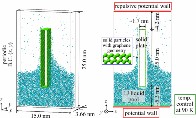
Figure 1: Equilibrium molecular dynamics (MD) simulation systems of a quasi-2D meniscus formed on a hollow rectangular solid plate dipped into a liquid pool of a simple Lennard-Jones (LJ) fluid: the Wilhelmy MD system.

We employed equilibrium MD simulation systems of a quasi-2D meniscus formed on a hollow rectangular solid plate (denote by ‘solid plate’ hereafter) dipped into a liquid pool of a simple fluid as shown in Fig. 1. We call this system the ‘Wilhelmy MD system’ hereafter. Generic particles interacting through a LJ potential were adopted as the fluid particles. The 12-6 LJ potential given by

$$\Phi^{\mathrm{LJ}}(r_{ij})=4\epsilon\left[\left(\frac{\sigma}{r_{ij}}\right)^{12}-\left(\frac{\sigma}{r_{ij}}\right)^{6}+c_{2}^{\mathrm{LJ}}\left(\frac{r_{ij}}{r_{\mathrm{c}}}\right)^{2}+c_{0}^{\mathrm{LJ}}\right],$$ (5)

was used for the interaction between fluid particles, where $r_{ij}$ is the distance between the particles $i$ at position $\mbox{\boldmath$r$}_{i}$ and $j$ at $\mbox{\boldmath$r$}_{j}$, while $\epsilon$ and $\sigma$ denote the LJ energy and length parameters, respectively. This LJ interaction was truncated at a cut-off distance of $r_{\mathrm{c}}=3.5\sigma$ and quadratic functions were added so that the potential and interaction force smoothly vanished at $r_{\mathrm{c}}$. The constant values of $c_{2}^{\mathrm{LJ}}$ and $c_{0}^{\mathrm{LJ}}$ were given in our previous study. Nishida et al. (2014) Hereafter, fluid and solid particles are denoted by ‘f’ and ‘s’, respectively and corresponding combinations are indicated by subscripts.

A rectangular solid plate in contact with the fluid was prepared by bending a honeycomb graphene sheet, where the solid particles were fixed on the coordinate with the positions of 2D-hexagonal periodic structure with an inter-particle distance $r_{\mathrm{ss}}$ of 0.141 nm. The zigzag edge of the honeycomb structure was set parallel to the $y$-direction with locating solid particles at the edge to match the hexagonal periodicity. The right and left faces were set at $x=\pm x_{\mathrm{s}}$ parallel to the $yz$-plane, and the top and bottom faces were parallel to the $xy$-plane. Note that the distance between the left and right faces $2x_{\mathrm{s}}\approx 1.7$ nm was larger than the cutoff distance $r_{\mathrm{c}}$.

The solid-fluid (SF) interaction, which denotes SL or SV interaction, was also expressed by the LJ potential in Eq. (5), where the length parameter $\sigma_{\mathrm{sf}}$ was given by the Lorentz mixing rule, while the energy parameter $\epsilon_{\mathrm{sf}}$ was changed in a parametric manner by multiplying a SF interaction coefficient $\eta$ to the base value $\epsilon^{0}_{\mathrm{sf}}=\sqrt{\epsilon_{\mathrm{ff}}\epsilon_{\mathrm{ss}}}$ as

$$\epsilon_{\mathrm{sf}}=\eta\epsilon^{0}_{\mathrm{sf}}.$$ (6)

This parameter $\eta$ expressed the wettability, i.e., $\eta$ and the contact angle of a hemi-cylindrically shaped equilibrium droplet on a homogeneous flat solid surface had a one-to-one correspondence Nishida et al. (2014); Yamaguchi et al. (2019); Kusudo, Omori, and Yamaguchi (2019), and we set the parameter $\eta$ between 0.03 and 0.15 so that the corresponding cosine of the contact angle $\cos\theta$ may be from $-0.9$ to $0.9$. The definition of the contact angle is described later in Sec. III. Note that due to the fact that the solid-solid inter-particle distance $r_{\mathrm{ss}}$ shown in Table 1 were relatively small compared to the LJ length parameters $\sigma_{\mathrm{ff}}$ and $\sigma_{\mathrm{fs}}$, the surface is considered to be very smooth, and the wall-tangential force from the solid on the fluid, which induces pinning of the CL, is negligible. Yamaguchi et al. (2019); Kusudo, Omori, and Yamaguchi (2019)

In addition to these intermolecular potentials, we set a horizontal potential wall on the bottom (floor) of the calculation cell fixed at $z=z_{\mathrm{flr}}$ about 5.3 nm below the bottom of the solid plate, which interacted only with the fluid particles with a one-dimensional potential field $\Phi_{\mathrm{flr}}^{\mathrm{1D}}$ as the function of the distance from the wall given by

$$\Phi_{\mathrm{flr}}^{\mathrm{1D}}(z^{\prime}_{i})=4\pi\rho_{n}\epsilon^{0}_{\mathrm{sf}}\sigma_{\mathrm{sf}}^{2}\left[\frac{1}{5}\left(\frac{\sigma_{\mathrm{sf}}}{z^{\prime}_{i}}\right)^{10}\!\!\!\!-\frac{1}{2}\left(\frac{\sigma_{\mathrm{sf}}}{z^{\prime}_{i}}\right)^{4}+c_{2}^{\mathrm{flr}}\left(\frac{z^{\prime}_{i}}{z_{\mathrm{c}}^{\mathrm{flr}}}\right)^{2}+c_{1}^{\mathrm{flr}}\left(\frac{z^{\prime}_{i}}{z_{\mathrm{c}}^{\mathrm{flr}}}\right)+c_{0}^{\mathrm{flr}}\right],\quad z^{\prime}_{i}\equiv z_{i}-z_{\mathrm{flr}}$$ (7)

where $z_{i}$ is the $z$-position of fluid particle $i$. This potential wall mimicked a mean potential field created by a single layer of solid particles with a uniform area number density $\rho_{n}$. Similar to Eq. (5), this potential field in Eq. (7) was truncated at a cut-off distance of $z_{\mathrm{c}}^{\mathrm{flr}}=3.5\sigma_{\mathrm{sf}}$ and a quadratic function was added so that the potential and interaction force smoothly vanished at $z_{\mathrm{c}}^{\mathrm{flr}}$. As shown in Fig. 1, fluid particles were rather strongly attracted on this plane because this roughly corresponded to a solid wall showing complete wetting. With this setup, the liquid pool was stably kept even when the liquid pressure is low with a highly wettable solid plate. Furthermore, we set another horizontal potential wall on the top (ceiling) of the calculation cell fixed at $z=z_{\mathrm{ceil}}$ about 4.7 nm above the top of the solid plate exerting a repulsive potential field $\Phi_{\mathrm{ceil}}^{\mathrm{1D}}$ on the fluid particles given by

$$\Phi_{\mathrm{ceil}}^{\mathrm{1D}}(z^{\prime\prime}_{i})=4\pi\rho_{n}\epsilon^{0}_{\mathrm{sf}}\sigma_{\mathrm{sf}}^{2}\left[\frac{1}{5}\left(\frac{\sigma_{\mathrm{sf}}}{z^{\prime\prime}_{i}}\right)^{10}+c_{2}^{\mathrm{ceil}}\left(\frac{z^{\prime\prime}_{i}}{z_{\mathrm{c}}^{\mathrm{ceil}}}\right)^{2}+c_{1}^{\mathrm{ceil}}\left(\frac{z^{\prime\prime}_{i}}{z_{\mathrm{c}}^{\mathrm{ceil}}}\right)+c_{0}^{\mathrm{ceil}}\right],\quad z^{\prime\prime}_{i}\equiv z_{\mathrm{ceil}}-z_{i},$$ (8)

where a cut-off distance of $z_{\mathrm{c}}^{\mathrm{ceil}}=\sigma_{\mathrm{sf}}$ was set to express a repulsive potential wall.

The periodic boundary condition was set in the horizontal $x$- and $y$-directions, where the system size in the $y$-direction $l_{y}\approx 3.66$ nm matched the hexagonal periodicity of the graphene sheet. The temperature of the system was maintained at a constant temperature of $T_{\mathrm{c}}$ at 90 K, which was above the triple point temperature, Mastny and de Pablo (2007) by velocity rescaling applied to the fluid particles within 0.8 nm from the floor wall regarding the velocity components in the $x$- and $y$-directions. Note that this region was sufficiently away from the bottom of the solid plate and no direct thermostating was imposed on around the solid plate, so that this temperature control had no effects on the present results.

With this setting, a quasi-2D LJ liquid of a meniscus-shaped LV interface with the CL parallel to the $y-$direction was formed as an equilibrium state as exemplified in Fig. 1, where a liquid bulk with an isotropic density distribution existed above the bottom wall by choosing a proper number of fluid particles $N_{\mathrm{f}}$ as shown in Fig. 2. We checked that the temperature was constant in the whole system after the equilibration run described below. Note also that in the present quasi-2D systems, effects of the CL curvature can be neglected. Boruvka and Neumann (1977); Marmur (1997); Ingebrigtsen and Toxvaerd (2007); Leroy and Müller-Plathe (2010); Weijs et al. (2011); Nishida et al. (2014); Yamaguchi et al. (2019); Kusudo, Omori, and Yamaguchi (2019) The velocity Verlet method was applied for the integration of the Newtonian equation of motion with a time increment of 5 fs for all systems. The simulation parameters are summarized in Table 1 with the corresponding non-dimensional ones, which are normalized by the corresponding standard values based on $\epsilon_{\mathrm{ff}}$, $\sigma_{\mathrm{ff}}$ and $m_{\mathrm{f}}$.

The physical properties of each equilibrium system with various $\eta$ values were calculated as the time average of 40 ns, which followed an equilibration run of more than 10 ns.

Table 1: Simulation parameters and their corresponding non-dimensional values.

property	value	unit	non-dim. value
$\sigma_{\mathrm{ff}}$	0.340	nm	1
$\sigma_{\mathrm{sf}}$	0.357	nm	1.05
$\epsilon_{\mathrm{ff}}$	$1.67\times 10^{-21}$	J	1
$\epsilon^{0}_{\mathrm{sf}}$	$1.96\times 10^{-21}$	J	1.18
$\epsilon_{\mathrm{sf}}$	$\eta\times\epsilon^{0}_{\mathrm{sf}}$
$\eta$	0.03 – 0.15	-	-
$m_{\mathrm{f}}$	$6.64\times 10^{-26}$	kg	1
$T_{\mathrm{c}}$	90	K	0.703
$N_{\mathrm{f}}$	10000 - 15000	-	-

III Results and discussion

III.1 Contact angle and force on the solid plate

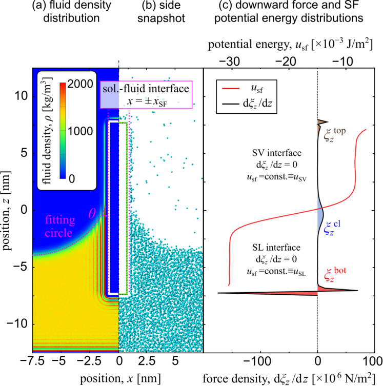
Figure 2: (a) Distribution of the time-averaged fluid density, (b) half side snapshot, and (c) distributions of the time-averaged downward force density acting on the solid plate and solid-fluid (SF) potential energy for the system with a SF interaction parameter $\eta$ of 0.15.

We calculated the distribution of force exerted from the fluid on the solid particles by dividing the system into equal-sized bins normal to the $z$-direction, where the height of the bin $\delta z$ of 0.2115 nm was used considering the periodicity of the graphene structure. We defined the average force density $\mathrm{d}\xi_{z}/\mathrm{d}z$ as the time-averaged total downward (in $-z$-direction) force from the fluid on the solid particles in each bin divided by $2l_{y}\delta z$, where $l_{y}$ is the system width in the $y$-direction. Except at the top and bottom of the solid plate, $\mathrm{d}\xi_{z}/\mathrm{d}z$ corresponds to the total downward force from both sides divided by the sum of surface area of both sides, i.e., the downward force per surface area. We also calculated the average SF potential energy per area $u_{\mathrm{sf}}$ as well, which was obtained by substituting the downward force by the SF potential energy.

Figure 2 shows the distribution of time-averaged fluid density $\rho$ around the solid plate for the system with solid-fluid interaction parameter $\eta=0.15$ and a snapshot of the system. The time-averaged distributions of the downward force acting on the solid plate $\mathrm{d}\xi_{z}/\mathrm{d}z$ and the SF potential energy $u_{\mathrm{sf}}$ are also displayed in the right panel. Multi-layered structures in the liquid, called the adsorption layers, were formed around the solid plate and the potential wall on the bottom, and liquid bulk with a homogeneous density is observed away from the potential wall, the solid plate and the LV interface.

The downward force $\mathrm{d}\xi_{z}/\mathrm{d}z$ on the solid plate in Fig. 2 (c) was positive around the top as filled with brown, zero below the top up to around the CL, and had smoothly distributed positive values around the CL as filled with blue. As further going downward, it became zero again below around the CL, and showed sharp change from positive to negative values as filled with red. On the SV interface between the plate top and CL and on the SL interface between the CL and the plate bottom, the time-averaged downward force was zero. Regarding the SF potential energy, $u_{\mathrm{sf}}$ was constant in the region where $\mathrm{d}\xi_{z}/\mathrm{d}z=0$. This is because the time-averaged fluid density in these regions was homogeneous in the $z$-direction, i.e., $\partial\rho/\partial z=0$ was satisfied within the range where the intermolecular force from the fluid on the solid particles effectively reaches, and no surface-tangential force in the $z$-direction was exerted on the solid. This point will be described more in detail in Subsec. III.2. Such two regions with zero downward force were formed for all systems in the present study, and thus, the total downward force as the integral of $\mathrm{d}\xi_{z}/\mathrm{d}z$ can be clearly separated into three local parts, i.e., $\xi_{z}^{\mathrm{top}}$ around the top, $\xi_{z}^{\mathrm{cl}}$ around the contact line, and $\xi_{z}^{\mathrm{bot}}$ around the bottom. As indicated in Fig 2 (c), $\xi_{z}^{\mathrm{top}}$ and $\xi_{z}^{\mathrm{cl}}$ are positive, i.e., downward forces, and $\xi_{z}^{\mathrm{bot}}$ is negative, i.e., an upward force. Note that the distributions of $\mathrm{d}\xi_{z}/\mathrm{d}z$ and $u_{\mathrm{sf}}$ around the top and bottom had less physical meaning because they included the top and bottom faces in the bin, and these parts for $u_{\mathrm{sf}}$ are not displayed in the figure. However, the local integral of $\mathrm{d}\xi_{z}/\mathrm{d}z$ indeed gave the physical information about the force around the top and bottom parts. Note also that $\xi_{z}$ has the same dimension as the surface tension of force per length.

The LV interface had a uniform curvature away from the solid plate to minimize LV interface area as one of the principal properties of surface tension. Considering the symmetry of the system, the hemi-cylindrical LV interface with a uniform curvature is symmetrical between the solid plates over the periodic boundary in the $x$-direction. Regarding SF interface position $x_{\mathrm{SF}}$, which was different from the wall surface position $x_{s}$, we defined it at the limit that the fluid could reach. With this definition, Young’s equation holds for quasi-2D droplets on a smooth and flat solid surface, as shown in our previous study. Yamaguchi et al. (2019) The $x_{\mathrm{SF}}$ value was determined as $x_{\mathrm{SF}}=1.15$ nm from the density distribution, whereas the curvature radius $R$ was determined through the least-squares fitting of a circle on the density contour of $\rho=$400 kg/m³ at the LV interface excluding the region in the adsorption layers near the solid surface. Nishida et al. (2014); Yamaguchi et al. (2019); Kusudo, Omori, and Yamaguchi (2019) We defined the apparent contact angle $\theta$ by the angle at $x=x_{\mathrm{SF}}$ between the SF interface and the least-squares fit of the LV interface having a curvature $\chi\equiv\pm 1/R$, with $R$ being the curvature radius. Note that the sign $\pm$ corresponds to the downward or upward convex LV-interfaces, respectively. The relation between the SF interaction coefficient $\eta$ and cosine of the contact angle $\cos\theta$ is shown in Appendix A, and the following results are shown based on $\cos\theta$ instead of $\eta$.

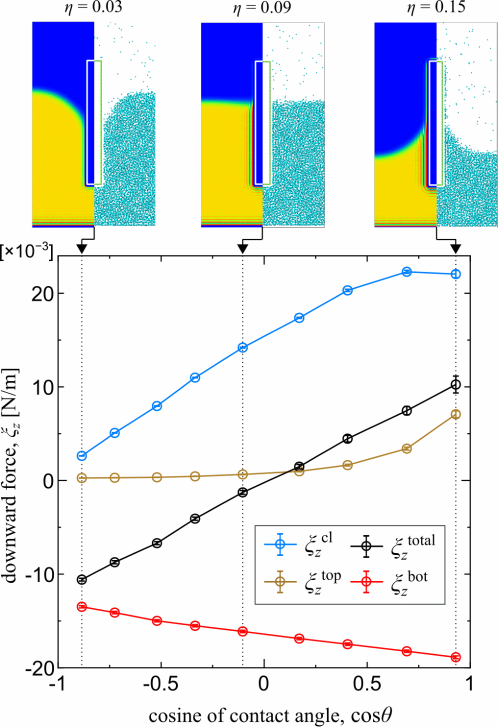
Figure 3: MD results of the local downward forces exerted around the top, the contact line and the bottom of the solid plate and their sum as a function of the cosine of the contact angle. Corresponding half-snapshots and density distributions for three cases are also displayed on the top.

Figure 3 shows the above-defined local downward forces $\xi_{z}^{\mathrm{top}}$, $\xi_{z}^{\mathrm{cl}}$ and $\xi_{z}^{\mathrm{bot}}$ and their sum $\xi_{z}^{\mathrm{total}}\equiv\xi_{z}^{\mathrm{top}}+\xi_{z}^{\mathrm{cl}}+\xi_{z}^{\mathrm{bot}}$ on the cosine of the contact angle $\cos\theta$ obtained by MD simulations. Corresponding half-snapshots and density distributions are also displayed on the top. Regarding the force around the top $\xi_{z}^{\mathrm{top}}$, it was almost zero except for cases with small contact angle. This is obvious because almost no vapor particles were adsorbed on the top of the solid plate for non-wetting cases as seen in the top panel for $\eta=0.03$. However, in the case of large $\cos\theta$, $\xi_{z}^{\mathrm{top}}$ had non-negligible positive value, i.e., downward force comparable to $\xi_{z}^{\mathrm{total}}$, because an adsorption layer was also formed at the SV interface as seen in the top panel for $\eta=0.15$. In terms of the force around the contact line $\xi_{z}^{\mathrm{cl}}$, it was positive even with negative $\cos\theta$ value, meaning that the solid particle around the CL was always subject to a downward force from the fluid. On the contrary to $\xi_{z}^{\mathrm{top}}$ and $\xi_{z}^{\mathrm{cl}}$, which were both positive, $\xi_{z}^{\mathrm{bot}}$ was negative and its magnitude increased as $\cos\theta$ increased, meaning that upward force to expel the bottom side was exerted from the liquid, and that the upward force was larger for larger SL interaction $\eta$. Finally, the sum of the above three $\xi_{z}^{\mathrm{total}}$ seems to be proportional to $\cos\theta$. We will show later that it actually deviates from a simple Wilhelmy relation (3).

III.2 Analytical expressions of the forces on the solid

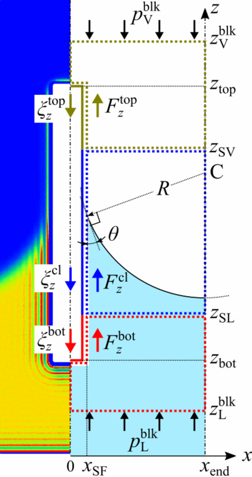
Figure 4: Top, contact-line (middle), and bottom parts of the solid plate subject to downward forces $\xi_{z}^{\mathrm{top}}$, $\xi_{z}^{\mathrm{cl}}$ and $\xi_{z}^{\mathrm{bot}}$ from the fluid, respectively, and the control volumes (CVs) surrounding the fluid particles in contact with these solid parts subject to upward force $F_{z}^{\mathrm{top}}$, $F_{z}^{\mathrm{cl}}$ and $F_{z}^{\mathrm{bot}}$ from the solid.

III.2.1 Definition of the solid-fluid forces

In order to elucidate the origin of the forces exerted on the solid, we examined the details of the forces $\xi_{z}^{\mathrm{top}}$, $\xi_{z}^{\mathrm{cl}}$ and $\xi_{z}^{\mathrm{bot}}$ from the fluid as well as the force balance on the control volumes (CVs) surrounding the fluid around the solid plate with taking the stress distribution in the fluid into account as in our previous study. Yamaguchi et al. (2019); Kusudo, Omori, and Yamaguchi (2019) We supposed three CVs surrounding the fluid around the solid plate as shown with dotted lines in Fig. 4: a CV on the top in dark-yellow dotted line, one around the CL in blue dotted line, and one on the bottom in red dotted line. All the CVs have their right face at the boundary of the system in the $x$-direction at $x=x_{\mathrm{end}}$ at which symmetry of the physical values is satisfied, and the faces in contact with the solid is set at the limit that the fluid could reach. The remaining left sides of the top and bottom CVs are set in the center of the system where the symmetry condition is satisfied. The $z$-normal faces are set respectively at $z=z_{\mathrm{V}}^{\mathrm{blk}}$, $z_{\mathrm{SV}}$, $z_{\mathrm{SL}}$ and $z_{\mathrm{L}}^{\mathrm{blk}}$, where $z_{\mathrm{V}}^{\mathrm{blk}}$ and $z_{\mathrm{L}}^{\mathrm{blk}}$ are at the vapor and liquid bulk heights, whereas $z_{\mathrm{SV}}$ and $z_{\mathrm{SL}}$ are set at the heights of SV and SL interfaces, respectively as shown in Fig. 3 at which $\mathrm{d}\xi_{z}/\mathrm{d}z=0$ is satisfied. These heights can be set rather arbitrary as long as the above conditions are satisfied. We define the forces from solid to liquid by $F_{z}^{\mathrm{top}}$, $F_{z}^{\mathrm{cl}}$ and $F_{z}^{\mathrm{bot}}$ on the top, middle and bottom CVs, respectively. In addition, we also categorize the right-half of the solid plate into top, middle and bottom parts shown with dark-yellow, blue, and red solid lines, respectively with $z_{\mathrm{SV}}$ and $z_{\mathrm{SL}}$ as the boundaries as shown in Fig. 4. where forces $\xi_{z}^{\mathrm{top}}$, $\xi_{z}^{\mathrm{cl}}$ and $\xi_{z}^{\mathrm{bot}}$ in the $z$-direction are exerted from the fluid, respectively. Specifically note that $\xi_{z}^{\mathrm{cl}}\neq F_{z}^{\mathrm{cl}}$, $\xi_{z}^{\mathrm{bot}}\neq F_{z}^{\mathrm{bot}}$ and $\xi_{z}^{\mathrm{top}}\neq F_{z}^{\mathrm{top}}$, because, for instance, $F_{z}^{\mathrm{cl}}$ also includes the forces from the top and bottom parts of the solid, whereas $\xi_{z}^{\mathrm{cl}}$ includes the forces from the top and bottom CVs. In other words, the force between the middle solid part and middle fluid CV is in action-reaction relation, but $F_{z}^{\mathrm{cl}}$ and $\xi_{z}^{\mathrm{cl}}$ include different extra forces above. This will be described more in detail in the following.

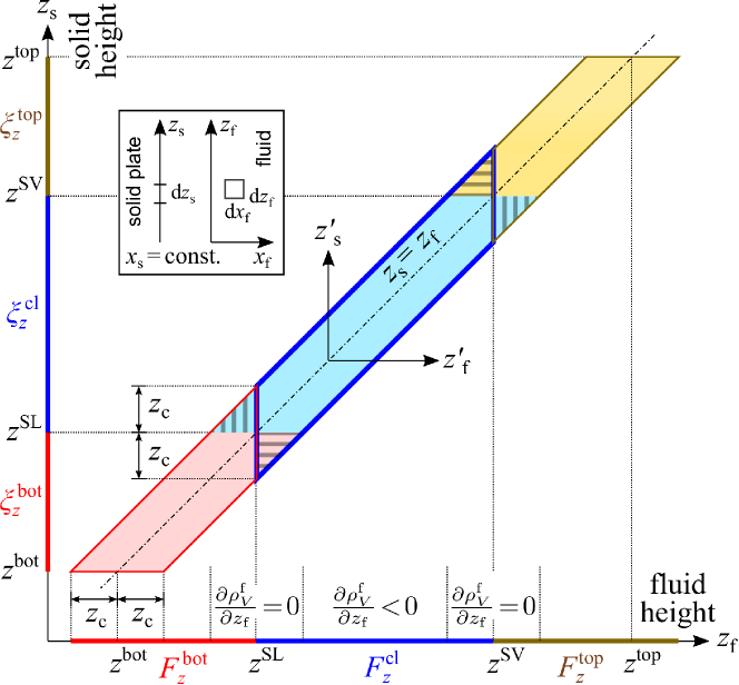
Figure 5: Region for the double integral of the mean field regarding the interaction between solid plate and fluid at height $z_{\mathrm{s}}$ and $z_{\mathrm{f}}$, respectively. The geometrical relation is shown in the inset. Three height ranges of ‘top,’ ‘cl,’ and ‘bot’ corresponding to those in Fig. 4 are depicted in color. Cutoff distance $z_{\mathrm{c}}$ for $|z_{\mathrm{f}}-z_{\mathrm{s}}|$ is set depending on the lateral position $x_{\mathrm{f}}-x_{\mathrm{s}}$, and the solid-liquid interactions between height ranges are categorized as filled regions or as ones surrounded by solid lines.

III.2.2 Capillary force $\xi_{z}^{\mathrm{cl}}$ around the contact line based on a mean-field approach

We start from formulating the wall tangential force on the solid particles $\xi_{z}^{\mathrm{cl}}$ on the right face of the solid plate. Taking into account that the solid is supposed to be smooth for the fluid particles because the interparticle distance parameters $\sigma_{\mathrm{ff}}$ and $\sigma_{\mathrm{sf}}$ are sufficiently large compared to $r_{\mathrm{ss}}$ between solid particles, $\xi_{z}^{\mathrm{cl}}$ can be analytically modeled by assuming the mean fields of the fluid and solid. The mean number density per volume $\rho_{V}^{\mathrm{f}}(z_{\mathrm{f}},x_{\mathrm{f}})\ (=\rho/m_{\mathrm{f}})$ of the fluid is given as a function of the two-dimensional position $(z_{\mathrm{f}},x_{\mathrm{f}})$ of the fluid, whereas a constant mean number density per area $\rho_{A}^{\mathrm{s}}$ of the solid is used considering the present system with a solid plate of zero-thickness without volume; however, the following derivation can easily be extended for a system with a solid with a volume and density per volume in the range $x\leq x_{\mathrm{s}}$ as long as the density is independent of $z_{\mathrm{s}}$. We start from the potential energy on a solid particle at position $(x_{\mathrm{s}},y_{\mathrm{s}},z_{\mathrm{s}})$ due to a fluid particle at $(x_{\mathrm{f}},y_{\mathrm{f}},z_{\mathrm{f}})$ given by Eq. (5). We define

$$x{{}^{\prime}}_{\mathrm{f}}=-x{{}^{\prime}}_{\mathrm{s}}\equiv x_{\mathrm{f}}-x_{\mathrm{s}},\quad y{{}^{\prime}}_{\mathrm{f}}=-y{{}^{\prime}}_{\mathrm{s}}\equiv y_{\mathrm{f}}-y_{\mathrm{s}},\quad z{{}^{\prime}}_{\mathrm{f}}=-z{{}^{\prime}}_{\mathrm{s}}\equiv z_{\mathrm{f}}-z_{\mathrm{s}}$$ (9)

in the following. Assuming that the fluid particles are homogeneously distributed in the $y$-direction with a number density $\rho_{V}^{\mathrm{f}}(z_{\mathrm{f}},x_{\mathrm{f}})$ per volume, the mean potential field from an infinitesimal volume segment of $\mathrm{d}z_{\mathrm{f}}\times\mathrm{d}x_{\mathrm{f}}$ on the solid particle is defined by using $\rho_{V}^{\mathrm{f}}(z_{\mathrm{f}},x_{\mathrm{f}})$ and the mean local potential $\phi(z{{}^{\prime}}_{\mathrm{f}},x{{}^{\prime}}_{\mathrm{f}})$ as $\rho_{V}^{\mathrm{f}}(z_{\mathrm{f}},x_{\mathrm{f}})\mathrm{d}z_{\mathrm{f}}\mathrm{d}x_{\mathrm{f}}\cdot\phi(z{{}^{\prime}}_{\mathrm{f}},x{{}^{\prime}}_{\mathrm{f}})$, where $\phi(z{{}^{\prime}}_{\mathrm{f}},x{{}^{\prime}}_{\mathrm{f}})$ is given by

$$\phi(z{{}^{\prime}}_{\mathrm{f}},x{{}^{\prime}}_{\mathrm{f}})\equiv\int_{-\infty}^{\infty}\Phi_{\mathrm{LJ}}(r)\mathrm{d}y{{}^{\prime}}_{\mathrm{f}}$$ (10)

with

$$r=\sqrt{x{{}^{\prime}}_{\mathrm{f}}^{2}+y{{}^{\prime}}_{\mathrm{f}}^{2}+z{{}^{\prime}}_{\mathrm{f}}^{2}},\quad\sigma=\sigma_{\mathrm{sf}},\quad\epsilon=\epsilon_{\mathrm{sf}}.$$ (11)

This schematic is shown in the inset of Fig. 5. Then, the local tangential force $f_{z}^{\mathrm{s}}(z{{}^{\prime}}_{\mathrm{f}},x{{}^{\prime}}_{\mathrm{f}})\mathrm{d}z_{\mathrm{f}}\mathrm{d}x_{\mathrm{f}}\mathrm{d}z_{\mathrm{s}}$ exerted on an infinitesimal solid area-segment of $\mathrm{d}z_{\mathrm{s}}$ from the present fluid volume-segment is given by:

$$f_{z}^{\mathrm{s}}(z_{\mathrm{s}},z_{\mathrm{f}},x_{\mathrm{f}})\mathrm{d}z_{\mathrm{f}}\mathrm{d}x_{\mathrm{f}}\mathrm{d}z_{\mathrm{s}} =-\frac{\partial}{\partial z_{\mathrm{s}}}\left[\rho_{V}^{\mathrm{f}}(z_{\mathrm{f}},x_{\mathrm{f}})\phi(z{{}^{\prime}}_{\mathrm{f}},x{{}^{\prime}}_{\mathrm{f}})\right]\mathrm{d}z_{\mathrm{f}}\mathrm{d}x_{\mathrm{f}}\cdot\rho_{A}^{\mathrm{s}}\mathrm{d}z_{\mathrm{s}}$$

$$=-\rho_{A}^{\mathrm{s}}\rho_{V}^{\mathrm{f}}(z_{\mathrm{f}},x_{\mathrm{f}})\frac{\partial\phi(z{{}^{\prime}}_{\mathrm{f}},x{{}^{\prime}}_{\mathrm{f}})}{\partial z_{\mathrm{s}}}\mathrm{d}z_{\mathrm{f}}\mathrm{d}x_{\mathrm{f}}\mathrm{d}z_{\mathrm{s}},$$ (12)

where

$$f_{z}^{\mathrm{s}}(z_{\mathrm{s}},z_{\mathrm{f}},x_{\mathrm{f}})=-\rho_{A}^{\mathrm{s}}\rho_{V}^{\mathrm{f}}(z_{\mathrm{f}},x_{\mathrm{f}})\frac{\partial\phi(z{{}^{\prime}}_{\mathrm{f}},x{{}^{\prime}}_{\mathrm{f}})}{\partial z_{\mathrm{s}}}$$ (13)

denotes the tangential force density on the solid. Note that $\mathrm{d}x_{\mathrm{f}}$ and $\mathrm{d}x{{}^{\prime}}_{\mathrm{f}}$ are identical because $x_{\mathrm{s}}$ is a constant.

Since $\Phi_{\mathrm{LJ}}(r)$ is truncated at the cutoff distance $r_{\mathrm{c}}$ in the present case,

$$\phi\left(z{{}^{\prime}}_{\mathrm{f}},x{{}^{\prime}}_{\mathrm{f}}\right)=0,\quad\frac{\partial\phi\left(z{{}^{\prime}}_{\mathrm{f}},x{{}^{\prime}}_{\mathrm{f}}\right)}{\partial z_{\mathrm{s}}}=0$$ (14)

$$\mathrm{for}\quad|z{{}^{\prime}}_{\mathrm{f}}|\geq\sqrt{r_{\mathrm{c}}^{2}-x{{}^{\prime}}_{\mathrm{f}}^{2}}\equiv z_{\mathrm{c}}(x{{}^{\prime}}_{\mathrm{f}})\quad\mathrm{or}\quad x{{}^{\prime}}_{\mathrm{f}}\geq r_{\mathrm{c}}$$

holds, where $z_{\mathrm{c}}(x{{}^{\prime}}_{\mathrm{f}})$ as a function of $x{{}^{\prime}}_{\mathrm{f}}$ denotes the cutoff with respect to $z{{}^{\prime}}_{\mathrm{f}}$. Indeed this cutoff is not critical as long as $\phi\left(z{{}^{\prime}}_{\mathrm{f}},x{{}^{\prime}}_{\mathrm{f}}\right)$ quickly vanishes with the increase of $r$, but we continue the derivation including the cutoff for simplicity. With the definition of $x_{\mathrm{SF}}$ as the limit that the fluid could reach, it follows that

$$\rho_{V}^{\mathrm{f}}=0\quad\mathrm{for}\quad x_{\mathrm{f}}<x_{\mathrm{SF}}.$$ (15)

In addition, considering that $\phi(z{{}^{\prime}}_{\mathrm{f}},x{{}^{\prime}}_{\mathrm{f}})$ is an even function with respect to $z{{}^{\prime}}_{\mathrm{f}}$, i.e.,

$$\phi\left(z{{}^{\prime}}_{\mathrm{f}},x{{}^{\prime}}_{\mathrm{f}}\right)=\phi(-z{{}^{\prime}}_{\mathrm{f}},x{{}^{\prime}}_{\mathrm{f}}),$$ (16)

it follows for the mean local potential $\phi$ that

$$\frac{\partial\phi(z{{}^{\prime}}_{\mathrm{f}},x{{}^{\prime}}_{\mathrm{f}})}{\partial z_{\mathrm{s}}}=-\frac{\partial\phi(-z{{}^{\prime}}_{\mathrm{f}},x{{}^{\prime}}_{\mathrm{f}})}{\partial z_{\mathrm{s}}},$$ (17)

and

$$\frac{\partial\phi(z{{}^{\prime}}_{\mathrm{f}},x{{}^{\prime}}_{\mathrm{f}})}{\partial z_{\mathrm{s}}}=-\frac{\partial\phi(z{{}^{\prime}}_{\mathrm{f}},x{{}^{\prime}}_{\mathrm{f}})}{\partial z_{\mathrm{f}}},$$ (18)

where Eq. (9) is applied for the latter, which corresponds to the action-reaction relation between solid and fluid particles under a simple two-body interaction, i.e.,

$$f_{z}^{\mathrm{f}}(z_{\mathrm{s}},z_{\mathrm{f}},x_{\mathrm{f}})=-f_{z}^{\mathrm{s}}(z_{\mathrm{s}},z_{\mathrm{f}},x_{\mathrm{f}})=-\rho_{A}^{\mathrm{s}}\rho_{V}^{\mathrm{f}}(z_{\mathrm{f}},x_{\mathrm{f}})\frac{\partial\phi(z{{}^{\prime}}_{\mathrm{f}},x{{}^{\prime}}_{\mathrm{f}})}{\partial z_{\mathrm{f}}}$$ (19)

holds for the tangential force density on the fluid $f_{z}^{\mathrm{f}}$.

Based on these properties, we now derive the analytical expression of $\xi_{z}^{\mathrm{cl}}$ as the triple integral of the local tangential force $f_{z}^{\mathrm{s}}$ in Eq. (12) around the CL, where the fluid density $\rho_{V}^{\mathrm{f}}$ decreases with the increase of $z_{\mathrm{f}}$ within a certain range. Let this range be $z_{\mathrm{SL}}+z_{\mathrm{c}}\leq z_{\mathrm{f}}\leq z_{\mathrm{SV}}-z_{\mathrm{c}}$ satisfying

$$\frac{\partial\rho_{V}^{\mathrm{f}}}{\partial z_{\mathrm{f}}}<0\quad(z_{\mathrm{SL}}+z_{\mathrm{c}}\leq z_{\mathrm{f}}\leq z_{\mathrm{SV}}-z_{\mathrm{c}}),$$ (20)

and let $\rho_{V}^{\mathrm{f}}$ outside this range be given as a unique function of $x_{\mathrm{f}}$ by

$$\rho_{V}^{\mathrm{f}}(z_{\mathrm{f}},x_{\mathrm{f}})=\left\{\begin{array}[]{cc}\rho_{V}^{\mathrm{f(SL)}}(x_{\mathrm{f}})&(z_{\mathrm{SL}}-z_{\mathrm{c}}<z_{\mathrm{f}}<z_{\mathrm{SL}}+z_{\mathrm{c}})\\ \rho_{V}^{\mathrm{f(SV)}}(x_{\mathrm{f}})&(z_{\mathrm{SV}}-z_{\mathrm{c}}<z_{\mathrm{f}}<z_{\mathrm{SV}}+z_{\mathrm{c}})\end{array}\right.$$ (21)

as shown in Fig. 5. Then, $\xi_{z}^{\mathrm{cl}}$ is expressed by

$$\xi_{z}^{\mathrm{cl}}\equiv-\int_{x_{\mathrm{SF}}}^{x_{\mathrm{s}}+r_{\mathrm{c}}}\left[\int_{z_{\mathrm{SL}}}^{z_{\mathrm{SV}}}\left(\int_{-z_{\mathrm{c}}}^{z_{\mathrm{c}}}f_{z}^{\mathrm{s}}(z_{\mathrm{s}},z{{}^{\prime}}_{\mathrm{f}},x_{\mathrm{f}})\mathrm{d}z{{}^{\prime}}_{\mathrm{f}}\right)\mathrm{d}z_{\mathrm{s}}\right]\mathrm{d}x_{\mathrm{f}}$$ (22)

as the triple integral of the force density $f_{z}^{\mathrm{s}}$ in Eq. (13), where the integration range of the double integral regarding $z_{\mathrm{f}}$ and $z_{\mathrm{s}}$ corresponds to the region filled with blue in Fig. 5.

To obtain the double integral as the square brackets in Eq. (22) for the blue-filled region in Fig. 5, we calculate at first that in the region surrounded by the solid-blue line, add those in the vertically-hatched regions, and subtract those in the horizontally-hatched regions. Note that $\rho_{V}^{\mathrm{f}}(z_{\mathrm{f}},x_{\mathrm{f}})=\rho_{V}^{\mathrm{f(SL)}}(x_{\mathrm{f}})$ and $\rho_{V}^{\mathrm{f}}(z_{\mathrm{f}},x_{\mathrm{f}})=\rho_{V}^{\mathrm{f(SV)}}(x_{\mathrm{f}})$ are assumed for the hatched regions in the bottom-left and in the top-right regions, respectively based on Eq. (21). The double integral for the region surrounded by the solid-blue line is

$$\int_{z_{\mathrm{SL}}}^{z_{\mathrm{SV}}}\left(\int_{-z_{\mathrm{c}}}^{z_{\mathrm{c}}}f_{z}^{\mathrm{s}}\mathrm{d}z{{}^{\prime}}_{\mathrm{s}}\right)\mathrm{d}z_{\mathrm{f}} =-\rho_{A}^{\mathrm{s}}\int_{z_{\mathrm{SL}}}^{z_{\mathrm{SV}}}\!\!\!\!\rho_{V}^{\mathrm{f}}(z_{\mathrm{f}},x_{\mathrm{f}})\left(\int_{-z_{\mathrm{c}}}^{z_{\mathrm{c}}}\frac{\partial\phi(z{{}^{\prime}}_{\mathrm{f}},x{{}^{\prime}}_{\mathrm{f}})}{\partial z_{\mathrm{s}}}\mathrm{d}z{{}^{\prime}}_{\mathrm{s}}\right)\mathrm{d}z_{\mathrm{f}}$$

$$=0,$$ (23)

by using Eq. (16). Indeed, from Eq. (19), the reaction force $-F_{z}^{\mathrm{cl}}$ from solid on the fluid around the CL in the blue-dotted line in Fig. 4 is obtained by further integrating Eq. (23) with respect to $x_{\mathrm{f}}$, i.e.,

$$\int_{x_{\mathrm{SF}}}^{x_{\mathrm{s}}+r_{\mathrm{c}}}\left[\int_{z_{\mathrm{SL}}}^{z_{\mathrm{SV}}}\left(\int_{-z_{\mathrm{c}}}^{z_{\mathrm{c}}}f_{z}^{\mathrm{s}}\mathrm{d}z{{}^{\prime}}_{\mathrm{s}}\right)\mathrm{d}z_{\mathrm{f}}\right]\mathrm{d}x_{\mathrm{f}} =-\int_{x_{\mathrm{SF}}}^{x_{\mathrm{s}}+r_{\mathrm{c}}}\left[\int_{z_{\mathrm{SL}}}^{z_{\mathrm{SV}}}\left(\int_{-z_{\mathrm{c}}}^{z_{\mathrm{c}}}f_{z}^{\mathrm{f}}\mathrm{d}z{{}^{\prime}}_{\mathrm{s}}\right)\mathrm{d}z_{\mathrm{f}}\right]\mathrm{d}x_{\mathrm{f}}$$

$$=-F_{z}^{\mathrm{cl}}$$

$$=0.$$ (24)

The final equality means that no tangential force acts on the fluid there as mentioned in our previous study. Yamaguchi et al. (2019)

Regarding the bottom-left vertically-hatched region in Fig. 5, the double integral is

$$\int_{-z_{\mathrm{c}}}^{0}\left(\int_{-z{{}^{\prime}}_{\mathrm{f}}}^{z_{\mathrm{c}}}f_{z}^{\mathrm{s}}\mathrm{d}z{{}^{\prime}}_{\mathrm{s}}\right)\mathrm{d}z{{}^{\prime}}_{\mathrm{f}} =-\rho_{A}^{\mathrm{s}}\rho_{V}^{\mathrm{f(SL)}}(x_{\mathrm{f}})\int_{-z_{\mathrm{c}}}^{0}\left(\int_{-z{{}^{\prime}}_{\mathrm{f}}}^{z_{\mathrm{c}}}\frac{\partial\phi(z{{}^{\prime}}_{\mathrm{f}},x{{}^{\prime}}_{\mathrm{f}})}{\partial z_{\mathrm{s}}}\mathrm{d}z{{}^{\prime}}_{\mathrm{s}}\right)\mathrm{d}z{{}^{\prime}}_{\mathrm{f}}$$

$$=\rho_{A}^{\mathrm{s}}\rho_{V}^{\mathrm{f(SL)}}(x_{\mathrm{f}})\int_{-z_{\mathrm{c}}}^{0}\phi(z{{}^{\prime}}_{\mathrm{f}},x{{}^{\prime}}_{\mathrm{f}})\mathrm{d}z{{}^{\prime}}_{\mathrm{f}},$$ (25)

where $\phi(z_{\mathrm{c}},x{{}^{\prime}}_{\mathrm{f}})=0$ and Eq. (17) is used for the 2nd equality. This region physically corresponds to the interaction between blue solid part and fluid in the red-dotted part in Fig. 4. For the bottom-left horizontally-hatched region in Fig. 5, it follows that

$$\int_{0}^{z_{\mathrm{c}}}\left(\int_{-z_{\mathrm{c}}}^{-z{{}^{\prime}}_{\mathrm{f}}}f_{z}^{\mathrm{s}}\mathrm{d}z{{}^{\prime}}_{\mathrm{s}}\right)\mathrm{d}z_{\mathrm{f}} =-\rho_{A}^{\mathrm{s}}\rho_{V}^{\mathrm{f(SL)}}(x_{\mathrm{f}})\int_{0}^{z_{\mathrm{c}}}\left(\int_{-z_{\mathrm{c}}}^{-z{{}^{\prime}}_{\mathrm{f}}}\frac{\partial\phi(z{{}^{\prime}}_{\mathrm{f}},x{{}^{\prime}}_{\mathrm{f}})}{\partial z_{\mathrm{s}}}\mathrm{d}z{{}^{\prime}}_{\mathrm{s}}\right)\mathrm{d}z{{}^{\prime}}_{\mathrm{f}}$$

$$=-\rho_{A}^{\mathrm{s}}\rho_{V}^{\mathrm{f(SL)}}(x_{\mathrm{f}})\int_{0}^{z_{\mathrm{c}}}\phi(z{{}^{\prime}}_{\mathrm{f}},x{{}^{\prime}}_{\mathrm{f}})\mathrm{d}z{{}^{\prime}}_{\mathrm{f}}.$$ (26)

This region corresponds to the interaction between red solid part and fluid in the blue-dotted part in Fig. 4. Hence, the net force due to the double integral in the bottom-left hatched regions in Eqs. (25) and (26) with also integrating in the $x_{\mathrm{f}}$-direction, which we define by $u_{\mathrm{SL}}$, results in

$$u_{\mathrm{SL}}\equiv\rho_{A}^{\mathrm{s}}\int_{0}^{r_{\mathrm{c}}}\left(\rho_{V}^{\mathrm{f(SL)}}(x{{}^{\prime}}_{\mathrm{f}})\int_{-z_{\mathrm{c}}(x{{}^{\prime}}_{\mathrm{f}})}^{z_{\mathrm{c}}(x{{}^{\prime}}_{\mathrm{f}})}\phi(z{{}^{\prime}}_{\mathrm{f}},x{{}^{\prime}}_{\mathrm{f}})\mathrm{d}z{{}^{\prime}}_{\mathrm{f}}\right)\mathrm{d}x{{}^{\prime}}_{\mathrm{f}}.$$ (27)

As a physical meaning, $u_{\mathrm{SL}}$ represents the SL potential energy density i.e., potential energy per SL-interfacial area at the SL interface away from the CL and from the bottom of the solid plate.

Regarding the top-right hatched regions, the net force results in $-u_{\mathrm{SV}}$ with the SV potential energy density area given by

$$u_{\mathrm{SV}}\equiv\rho_{A}^{\mathrm{s}}\int_{0}^{r_{\mathrm{c}}}\left(\rho_{V}^{\mathrm{f(SV)}}(x{{}^{\prime}}_{\mathrm{f}})\int_{-z_{\mathrm{c}}(x{{}^{\prime}}_{\mathrm{f}})}^{z_{\mathrm{c}}(x{{}^{\prime}}_{\mathrm{f}})}\phi(z{{}^{\prime}}_{\mathrm{f}},x{{}^{\prime}}_{\mathrm{f}})\mathrm{d}z{{}^{\prime}}_{\mathrm{f}}\right)\mathrm{d}x{{}^{\prime}}_{\mathrm{f}},$$ (28)

which can be derived in a similar manner. Thus, it follows for the force $-\xi_{z}^{\mathrm{cl}}$ from the fluid on the solid around the CL that

$$-\xi_{z}^{\mathrm{cl}}=-F_{z}^{\mathrm{cl}}+u_{\mathrm{SL}}-u_{\mathrm{SV}},\quad\xi_{z}^{\mathrm{cl}}=F_{z}^{\mathrm{cl}}-u_{\mathrm{SL}}+u_{\mathrm{SV}},$$ (29)

therefore, by using $F_{z}^{\mathrm{cl}}=0$ in Eq. (24),

$$\xi_{z}^{\mathrm{cl}}=-u_{\mathrm{SL}}+u_{\mathrm{SV}}=(-u_{\mathrm{SL}})-(-u_{\mathrm{SV}})$$ (30)

is derived as the analytical expression of $\xi_{z}^{\mathrm{cl}}$, where the final expression is appended considering that the potential energy densities $u_{\mathrm{SL}}$ and $u_{\mathrm{SV}}$ are both negative.

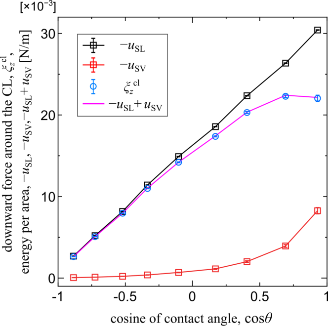
Figure 6: Dependence of the SL and SV potential density energy densities $u_{\mathrm{SL}}$ and $u_{\mathrm{SV}}$ as the potential energies per interfacial area on the cosine of the contact angle $\cos\theta$, and comparison between the force on the solid around the CL $\xi_{z}^{\mathrm{cl}}$ and difference of potential energy density $-u_{\mathrm{SL}}+u_{\mathrm{SV}}$.

Figure 6 shows the dependence of the SL and SV potential energy density $u_{\mathrm{SL}}$ and $u_{\mathrm{SV}}$, respectively as the potential energies per interfacial area, on the cosine of the contact angle $\cos\theta$, and comparison between the force on the solid around the CL $\xi_{z}^{\mathrm{cl}}$ and difference of potential energy density $-u_{\mathrm{SL}}+u_{\mathrm{SV}}$. Very good agreement between $\xi_{z}^{\mathrm{cl}}$ and $-u_{\mathrm{SL}}+u_{\mathrm{SV}}$ is observed within the whole range of the contact angle, and this indicates that Eq. 30 is applicable for the present system with a flat and smooth surface. It is also qualitatively apparent from Eq. (30) that $\xi_{z}^{\mathrm{cl}}$ is positive regardless of the contact angle because the SF potential energy is smaller at the SL interface than at the SV interface. It is also interesting to note that for the very wettable case with large $\cos\theta$, i.e., large wettability parameter $\eta$, $\xi_{z}^{\mathrm{cl}}$ decreased with the increase of $\cos\theta$. This can be explained as follows: the change of $-u_{\mathrm{SV}}$ and $-u_{\mathrm{SL}}$ are both due to the change of $\eta$ and the fluid density especially in the first adsorption layer, while the density change of the SL adsorption layer due to $\eta$ is rather small. Thus, for higher $\eta$ value, the effect of density increase of the SV adsorption layer on $-u_{\mathrm{SV}}$ upon the increase of $\eta$ overcomes the increase of $-u_{\mathrm{SL}}$.

III.2.3 Total force $\xi_{z}^{\mathrm{total}}$ and local forces $\xi_{z}^{\mathrm{bot}}$ and $\xi_{z}^{\mathrm{top}}$ on the bottom and the top

Before proceeding to the analytical expression of $\xi_{z}^{\mathrm{bot}}$ and $\xi_{z}^{\mathrm{top}}$, we derive their relations with $F_{z}^{\mathrm{bot}}$ and $F_{z}^{\mathrm{top}}$. Through the comparison between the regions of double integration for $\xi_{z}^{\mathrm{bot}}$ and $F_{z}^{\mathrm{bot}}$ with respect to $z_{\mathrm{f}}$ and $z_{\mathrm{s}}$ in Fig. 5, i.e., the red-filled region and one surrounded by solid-red line, it is clear that the difference between $\xi_{z}^{\mathrm{bot}}$ and $F_{z}^{\mathrm{bot}}$ corresponds to the integral of hatched regions around $z_{\mathrm{SL}}$ in the bottom-left. Thus, it follows that

$$\xi_{z}^{\mathrm{bot}}=F_{z}^{\mathrm{bot}}+u_{\mathrm{SL}}$$ (31)

and

$$\xi_{z}^{\mathrm{top}}=F_{z}^{\mathrm{top}}-u_{\mathrm{SV}}.$$ (32)

Note that the sum of Eqs. (30), (31) and (32) satisfies

$$\xi_{z}^{\mathrm{total}}=F_{z}^{\mathrm{top}}+F_{z}^{\mathrm{cl}}+F_{z}^{\mathrm{bot}}.$$ (33)

Considering that feature, we examine the total force $\xi_{z}^{\mathrm{total}}$ and local ones $\xi_{z}^{\mathrm{bot}}$ and $\xi_{z}^{\mathrm{top}}$ on the bottom and the top. We consider the distribution of the two-dimensional fluid stress tensor $\tau$ averaged in the $y$-direction by the method of plane (MoP) Thompson et al. (1984); Yaguchi, Yano, and Fujikawa (2010) based on the expression by Irving and Kirkwood (1950) (IK), with which exact force balance is satisfied for an arbitrary control volume bounded by a closed surface. The stress tensor component $\tau_{\alpha\beta}(x,z)$ denotes the stress in $\beta$-direction exerted on an infinitesimal surface element with an outward normal in $\alpha$-direction at position $(x,z)$. In the formulation of the MoP based on the IK-expression, $\tau_{\alpha\beta}(x,z)$ consists of the time-average of the kinetic and inter-molecular interaction contributions due to the molecular motion passing through the surface element and the intermolecular force crossing the surface element, respectively. For a single mono-atomic fluid component whose constituent particles interact through a pair potential as in the present study, all force line segments between two fluid particles, which cross the surface element, are included in the second. Note that technically for the MoP, the SF interaction can also be included in the inter-molecular force contribution, but only the FF interaction as the internal force is taken into account as the stress, and SF contribution is considered as an external force in this study. Nijmeijer et al. (1990); Schofield and Henderson (1982); Rowlinson (1993); Yamaguchi et al. (2019); Kusudo, Omori, and Yamaguchi (2019) With this setting, the stress is zero at the SF boundary for all CVs because no fluid particle exists beyond the boundary to contribute to the stress component as the kinetic nor at inter-molecular interaction contribution. Hence, the force balance on each CV containing only fluid is satisfied with the sum of the stress surface integral and external force from the solid. The force balance on the red-dotted CV in Fig. 4 in the $z$-direction is expressed by

$$-\int_{0}^{x_{\mathrm{end}}}\tau_{zz}(x,z_{\mathrm{L}}^{\mathrm{blk}})\mathrm{d}x+\int_{x_{\mathrm{SF}}}^{x_{\mathrm{end}}}\tau_{zz}(x,z_{\mathrm{SL}})\mathrm{d}x+F_{z}^{\mathrm{bot}}=0,$$ (34)

with the stress contributions from the bottom and top and external force in the RHS, respectively, by taking into account that $\tau_{xz}=0$ on the $x$-normal faces at $x=0$ and $x=x_{\mathrm{end}}$ due to the symmetry, and also that the stress at the SF interface is zero. Similarly, the force balance on the blue-dotted CV and dark-yellow-dotted CV in Fig. 4 in the $z$-direction are expressed by

$$-\int_{x_{\mathrm{SF}}}^{x_{\mathrm{end}}}\tau_{zz}(x,z_{\mathrm{SL}})\mathrm{d}x+\int_{x_{\mathrm{SF}}}^{x_{\mathrm{end}}}\tau_{zz}(x,z_{\mathrm{SV}})\mathrm{d}x+F_{z}^{\mathrm{cl}}=0,$$ (35)

and

$$-\int_{x_{\mathrm{SF}}}^{x_{\mathrm{end}}}\tau_{zz}(x,z_{\mathrm{SV}})\mathrm{d}x+\int_{0}^{x_{\mathrm{end}}}\tau_{zz}(x,z_{\mathrm{V}}^{\mathrm{blk}})\mathrm{d}x+F_{z}^{\mathrm{top}}=0,$$ (36)

respectively.

By taking the sum of Eqs. (34), (35) and (36), and inserting Eq. (33), it follows for $\xi_{z}^{\mathrm{total}}$ that

$$\xi_{z}^{\mathrm{total}}=\int_{0}^{x_{\mathrm{end}}}\tau_{zz}(x,z_{\mathrm{L}}^{\mathrm{blk}})\mathrm{d}x-\int_{0}^{x_{\mathrm{end}}}\tau_{zz}(x,z_{\mathrm{V}}^{\mathrm{blk}})\mathrm{d}x$$ (37)

Since the bottom face of the red-dotted CV and top face of the dark-yellow-dotted CV in Fig. 4 are respectively set in the liquid and vapor bulk regions under an isotropic static pressure $p_{\mathrm{L}}^{\mathrm{blk}}$, and $p_{\mathrm{V}}^{\mathrm{blk}}$ given by

$$p_{\mathrm{L}}^{\mathrm{blk}}=-\tau_{xx}(x,z_{\mathrm{L}}^{\mathrm{blk}})=-\tau_{zz}(x,z_{\mathrm{L}}^{\mathrm{blk}}),$$ (38)

and

$$p_{\mathrm{V}}^{\mathrm{blk}}=-\tau_{xx}(x,z_{\mathrm{V}}^{\mathrm{blk}})=-\tau_{zz}(x,z_{\mathrm{V}}^{\mathrm{blk}}),$$ (39)

the 1st and 2nd terms in the RHS of Eq. (37) write

$$\int_{0}^{x_{\mathrm{end}}}\tau_{zz}(x,z_{\mathrm{L}}^{\mathrm{blk}})\mathrm{d}x=-\int_{0}^{x_{\mathrm{end}}}p_{\mathrm{L}}^{\mathrm{blk}}\mathrm{d}x=-p_{\mathrm{L}}^{\mathrm{blk}}x_{\mathrm{end}},$$ (40)

and

$$\int_{0}^{x_{\mathrm{end}}}\tau_{zz}(x,z_{\mathrm{V}}^{\mathrm{blk}})\mathrm{d}x=-\int_{0}^{x_{\mathrm{end}}}p_{\mathrm{V}}^{\mathrm{blk}}\mathrm{d}x=-p_{\mathrm{V}}^{\mathrm{blk}}x_{\mathrm{end}}.$$ (41)

Thus, Eq. (37) results in a simple analytical expression of

$$\xi_{z}^{\mathrm{total}}=(p_{\mathrm{V}}^{\mathrm{blk}}-p_{\mathrm{L}}^{\mathrm{blk}})x_{\mathrm{end}}.$$ (42)

Furthermore, by applying the geometric relation

$$\sin\left(\theta-\frac{\pi}{2}\right)=\cos\theta=\chi\left(x_{\mathrm{end}}-x_{\mathrm{SF}}\right)$$ (43)

with $\chi$ being the LV interface curvature and the Young-Laplace equation for the pressure difference in Eq. (42):

$$p_{\mathrm{V}}^{\mathrm{blk}}-p_{\mathrm{L}}^{\mathrm{blk}}=\gamma_{\mathrm{LV}}\chi=\frac{\gamma_{\mathrm{LV}}\cos\theta}{x_{\mathrm{end}}-x_{\mathrm{SF}}},$$ (44)

which hold irrespective of whether the LV-interface is convex downward or upward, it follows for Eq. (42) as another analytical expression of $\xi_{z}^{\mathrm{total}}$ that

$$\xi_{z}^{\mathrm{total}}=\frac{x_{\mathrm{end}}}{x_{\mathrm{end}}-x_{\mathrm{SF}}}\gamma_{\mathrm{LV}}\cos\theta,$$ (45)

which includes the correction to Eq. (3) considering the effect of the Laplace pressure due to the finite system configuration with the periodic boundary condition. Note also that from Eq. (45), by giving $x_{\mathrm{end}}$ and $x_{\mathrm{SF}}$, it is possible to estimate $\gamma_{\mathrm{LV}}$ from the relation between $\xi_{z}^{\mathrm{total}}$ and $\cos\theta$.

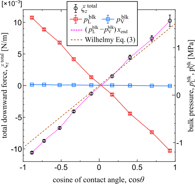
Figure 7: Comparison of the total downward force $\xi_{z}^{\mathrm{total}}$ on the solid plate directly obtained from MD with the analytical expression $(p_{\mathrm{V}}^{\mathrm{blk}}-p_{\mathrm{L}}^{\mathrm{blk}})x_{\mathrm{end}}$ in Eq. (42) using the pressures $p_{\mathrm{L}}^{\mathrm{blk}}$ and $p_{\mathrm{V}}^{\mathrm{blk}}$ measured on the bottom and top boundaries. The Wilhelmy equation (3) using $\gamma_{\mathrm{LV}}=9.79\times 10^{-3}$ N/m evaluated by the Young-Laplace equation (44) is also shown.

Figure 7 shows the comparison of the total downward force $\xi_{z}^{\mathrm{total}}$ on the solid plate directly obtained from MD with the analytical expression $(p_{\mathrm{V}}^{\mathrm{blk}}-p_{\mathrm{L}}^{\mathrm{blk}})x_{\mathrm{end}}$ in Eq. (42) using the pressures $p_{\mathrm{L}}^{\mathrm{blk}}$ and $p_{\mathrm{V}}^{\mathrm{blk}}$ measured on the bottom and top boundaries as the force exerted from the fluid on the potential walls per area. Clearly $\xi_{z}^{\mathrm{total}}$ and $(p_{\mathrm{V}}^{\mathrm{blk}}-p_{\mathrm{L}}^{\mathrm{blk}})x_{\mathrm{end}}$ agree very well, and this is because Eq. (42) is simply the force balance to be satisfied for equilibrium systems. Regarding the pressure, $p_{\mathrm{V}}^{\mathrm{blk}}$ is almost constant, which corresponds to the saturated vapor pressure at this temperature. In addition, a linear relation between $p_{\mathrm{L}}^{\mathrm{blk}}-p_{\mathrm{V}}^{\mathrm{blk}}$ and $\cos\theta$ can be observed, and this indicates that the Young-Laplace equation (44) is applicable in the present scale. We evaluated $\gamma_{\mathrm{LV}}$ from this relation with the least-squares fitting, and the resulting value was $\gamma_{\mathrm{LV}}=9.79\pm 0.23\times 10^{-3}$ N/m with $x_{\mathrm{SF}}=1.15$ nm and $x_{\mathrm{end}}=7.5$ nm, which was indeed close to the value obtained by a standard mechanical process. Surblys et al. (2014) The standard Wilhelmy equation (3) using this value is also shown in Fig. 7, indicating that $\gamma_{\mathrm{LV}}$ would be overestimated with this standard Wilhelmy equation (3) in a small measurement system like the present one.

Finally, we derive the analytical expression of the local force $\xi_{z}^{\mathrm{bot}}$ and $\xi_{z}^{\mathrm{top}}$. For the derivation of $\xi_{z}^{\mathrm{bot}}$, we apply the extended Bakker’s equation for the SL relative interfacial tension Yamaguchi et al. (2019); Kusudo, Omori, and Yamaguchi (2019)

$$\gamma_{\mathrm{SL}}-\gamma_{\mathrm{S0}}=\int_{x_{\mathrm{SF}}}^{x_{\mathrm{end}}}\left[\tau_{zz}(x,z_{\mathrm{SL}})-\tau_{\mathrm{L}}^{\mathrm{blk}}\right]\mathrm{d}x$$ (46)

for the 2nd term in the LHS of Eq. (34), where $\gamma_{\mathrm{SL}}-\gamma_{\mathrm{S0}}$ is the SL interfacial tension relative to the interfacial tension between solid and fluid with only repulsive interaction (denoted by “0” to express the solid surface without adsorbed fluid particles). Then, it follows that

$$\int_{x_{\mathrm{SF}}}^{x_{\mathrm{end}}}\tau_{zz}(x,z_{\mathrm{SL}})\mathrm{d}x=\gamma_{\mathrm{SL}}-\gamma_{\mathrm{S0}}-(x_{\mathrm{end}}-x_{\mathrm{SF}})p_{\mathrm{L}}^{\mathrm{blk}}.$$ (47)

By inserting Eqs. (31), (40) and (47) into Eq. (34), the analytical expression of $\xi_{z}^{\mathrm{bot}}$ writes

$$\xi_{z}^{\mathrm{bot}} =-p_{\mathrm{L}}^{\mathrm{blk}}x_{\mathrm{end}}-[\gamma_{\mathrm{SL}}-\gamma_{\mathrm{S0}}-(x_{\mathrm{end}}-x_{\mathrm{SF}})p_{\mathrm{L}}^{\mathrm{blk}}]+u_{\mathrm{SL}}$$

$$=-x_{\mathrm{SF}}p_{\mathrm{L}}^{\mathrm{blk}}-(\gamma_{\mathrm{SL}}-\gamma_{\mathrm{S0}})+u_{\mathrm{SL}}.$$ (48)

Similary, by applying the Extended Bakker’s equation for the SV interfacial tension Yamaguchi et al. (2019); Kusudo, Omori, and Yamaguchi (2019)

$$\gamma_{\mathrm{SV}}-\gamma_{\mathrm{S0}}=\int_{x_{\mathrm{SF}}}^{x_{\mathrm{end}}}\left[\tau_{zz}(x,z_{\mathrm{SV}})-\tau_{\mathrm{V}}^{\mathrm{blk}}\right]\mathrm{d}x$$ (49)

to Eq. (36) with Eq. (32), the analytical expression of $\xi_{z}^{\mathrm{top}}$ writes

$$\xi_{z}^{\mathrm{top}}=x_{\mathrm{SF}}p_{\mathrm{V}}^{\mathrm{blk}}+(\gamma_{\mathrm{SV}}-\gamma_{\mathrm{S0}})-u_{\mathrm{SV}}.$$ (50)

To verify Eqs. (48) and (50), we compared the present results with $\xi_{z}^{\mathrm{bot}}$ and $\xi_{z}^{\mathrm{top}}$ calculated using the corresponding SL and SV works of adhesion $W_{\mathrm{SL}}$ and $W_{\mathrm{SV}}$ obtained by the thermodynamics integration (TI) with the dry-surface scheme. Leroy and Müller-Plathe (2015); Yamaguchi et al. (2019) The calculation detail is shown in Appendix B. By definition, the SL and SV interfacial tensions $\gamma_{\mathrm{SL}}$ and $\gamma_{\mathrm{SV}}$ are related to $W_{\mathrm{SL}}$ and $W_{\mathrm{SV}}$ by

$$W_{\mathrm{SL}}\equiv\gamma_{\mathrm{S0}}+\gamma_{\mathrm{L0}}-\gamma_{\mathrm{SL}}\approx\gamma_{\mathrm{S0}}+\gamma_{\mathrm{LV}}-\gamma_{\mathrm{SL}}$$ (51)

and

$$W_{\mathrm{SV}}\equiv\gamma_{\mathrm{S0}}+\gamma_{\mathrm{V0}}-\gamma_{\mathrm{SV}}\approx\gamma_{\mathrm{S0}}-\gamma_{\mathrm{SV}},$$ (52)

respectively, where the approximation $\gamma_{\mathrm{L0}}\approx\gamma_{\mathrm{LV}}$ for the interfacial tension $\gamma_{\mathrm{L0}}$ between liquid and vacuum is used in Eq. (51), and $\gamma_{\mathrm{V0}}$ is set zero in the final approximation in Eq. (52). Note that $\gamma_{\mathrm{L0}}$ or $\gamma_{\mathrm{LV}}$ is included in $W_{\mathrm{SL}}$. From Eqs. (51) and (48), and from Eqs. (52) and (50), $\xi_{z}^{\mathrm{bot}}$ and $\xi_{z}^{\mathrm{top}}$ are respectively rewritten by

$$\xi_{z}^{\mathrm{bot}}\approx W_{\mathrm{SL}}-p_{\mathrm{L}}^{\mathrm{blk}}x_{\mathrm{SF}}-\gamma_{\mathrm{LV}}+u_{\mathrm{SL}},$$ (53)

and

$$\xi_{z}^{\mathrm{top}}\approx x_{\mathrm{SF}}p_{\mathrm{V}}^{\mathrm{blk}}-W_{\mathrm{SV}}-u_{\mathrm{SV}}.$$ (54)

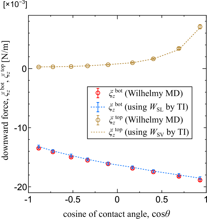
Figure 8: Comparison of the downward forces $\xi_{z}^{\mathrm{bot}}$ and $\xi_{z}^{\mathrm{top}}$ on the bottom and top of the solid plate directly obtained from MD with those evaluated using the works of adhesion $W_{\mathrm{SL}}$ and $W_{\mathrm{SV}}$ calculated by the thermodynamic integration (TI) using the dry-surface scheme shown in Appendix B. The error bar for $\xi_{z}^{\mathrm{bot}}$ using $W_{\mathrm{SL}}$ in blue comes from the evaluation of $\gamma_{\mathrm{LV}}$ from $p_{\mathrm{L}}^{\mathrm{blk}}$ and $p_{\mathrm{V}}^{\mathrm{blk}}$ in Fig. 7.

Figure 8 shows the comparison of $\xi_{z}^{\mathrm{bot}}$ and $\xi_{z}^{\mathrm{top}}$ directly obtained from MD with those evaluated by Eqs. (53) and (54) using the SL and SV works of adhesion $W_{\mathrm{SL}}$ and $W_{\mathrm{SV}}$, respectively obtained by the TI with the DS scheme shown in Appendix B. Note that except $W_{\mathrm{SL}}$ and $W_{\mathrm{SV}}$, we used the values of $p_{\mathrm{L}}^{\mathrm{blk}}$, $p_{\mathrm{V}}^{\mathrm{blk}}$, $x_{\mathrm{end}}$, $u_{\mathrm{SL}}$, and $u_{\mathrm{SV}}$ directly obtained from the present Wilhelmy MD simulations as well as the $\gamma_{\mathrm{LV}}$ value evaluated in Fig. 7. The error bars for $\xi_{z}^{\mathrm{bot}}$ using $W_{\mathrm{SL}}$ in blue mainly came from the error upon evaluating $\gamma_{\mathrm{LV}}$. Note also that the TI calculation in Appendix B for $W_{\mathrm{SL}}$ was carried out under a control pressure of 1 MPa whereas that for $W_{\mathrm{SV}}$ was considered to be under the saturated vapor pressure at the present temperature. For both $\xi_{z}^{\mathrm{bot}}$ and $\xi_{z}^{\mathrm{top}}$, the Wilhelmy MD and TI results agreed well, and this indicates the validity of the present analytical expression.

III.3 Discussion

We list the key issues for the further application of the present expression in the following. First, Eqs. (34), (35) and (36) are about the force balance and should be satisfied in equilibrium systems without any restrictions. In addition, Eqs. (29), (31) and (32) are about the relation between the solid-fluid and fluid-solid forces and should hold as long as the solid plate can be decomposed into the three parts without the interface overlapping. At both SL and SV interfaces, which are between the CL and the plate bottom and between CL and the plate top respectively, a quasi-one-dimensional density distribution with $\partial\rho/\partial z=0$ can be assumed and one can apply the mean-field approach described in Sec. III.2.2. Furthermore, Eqs. (46) and (49) are Extended Bakker’s equations Yamaguchi et al. (2019) for the SL and SV interfacial tensions. Hence, our analytical expressions with these equations are constructed by a purely mechanical approach, and are exact, as observed in the comparison in Figs. 6 and 7.

Another issue is about the relation between Young’s equation (1) and the Wilhelmy equation (42) formulated with the Laplace pressure. Indeed, Eq. (42) holds irrespective of whether the CL is pinned or not because this relation means a simple equilibrium force balance. In the present case, $F_{z}^{\mathrm{cl}}=0$ in Eq. (24) is satisfied because the solid surface is flat and smooth, and Young’s equation holds. This can easily be proved considering the force balance in Eq. (35) about the middle CV. In cases with $F_{z}^{\mathrm{cl}}\neq 0$ because of the pinning force exerted on the fluid from the solid around the CL, e.g., due to the boundary of wettability parallel to the CL in our previous research, Kusudo, Omori, and Yamaguchi (2019) Young’s equation should be rewritten including the pinning force. Even if such wettability boundary would be included in the present system, Eq. (42) would still be satisfied. In practice, such pinning force denoted by $\zeta_{\mathrm{pin}}$ in Ref. 22 as the downward force from the solid on the fluid around the CL corresponds to $-F_{z}^{\mathrm{cl}}$ here, and this can be extracted by Eq. (29) as

$$-\zeta_{\mathrm{pin}}=F_{z}^{\mathrm{cl}}=\xi_{z}^{\mathrm{cl}}+u_{\mathrm{SL}}-u_{\mathrm{SV}}.$$ (55)

Considering the above discussion, we summarize the procedure to extract the wetting properties. In a single Wilhelmy MD simulation, we can calculate

1. Force $\xi_{z}^{\mathrm{top}}$, $\xi_{z}^{\mathrm{cl}}$ and $\xi_{z}^{\mathrm{bot}}$ on three parts of the solid from the force-density distribution $\mathrm{d}\xi_{z}/\mathrm{d}z$ in the surface-tangential direction,

2. SF potential energy densities $u_{\mathrm{SL}}$ and $u_{\mathrm{SV}}$ on solid per area at SL and SV interfaces, respectively from the distribution of the potential energy density $u_{\mathrm{sf}}$,

3. Bulk pressures $p_{\mathrm{V}}^{\mathrm{blk}}$ and $p_{\mathrm{L}}^{\mathrm{blk}}$ measured on the top and bottom of the system, and

4. Contact angle $\theta$ from the density distribution.

From these quantities the following physical properties can be obtained:

1. SL relative interfacial tension $\gamma_{\mathrm{SL}}-\gamma_{\mathrm{S0}}$ from $\xi_{z}^{\mathrm{bot}}$, $u_{\mathrm{SL}}$, $x_{\mathrm{SF}}$ and $p_{\mathrm{L}}^{\mathrm{blk}}$ using Eq. (48),

2. SV relative interfacial tension $\gamma_{\mathrm{SV}}-\gamma_{\mathrm{S0}}$ from $\xi_{z}^{\mathrm{top}}$, $u_{\mathrm{SV}}$, $x_{\mathrm{SF}}$ and $p_{\mathrm{V}}^{\mathrm{blk}}$ using Eq. (50),

3. LV interfacial tension $\gamma_{\mathrm{LV}}$ from $p_{\mathrm{V}}^{\mathrm{blk}}$, $p_{\mathrm{L}}^{\mathrm{blk}}$, $x_{\mathrm{SF}}$, the system size $x_{\mathrm{end}}$ and the contact angle $\theta$ using Eq. (44) , and

4. Pinning force $F_{z}^{\mathrm{cl}}$ from Eq. (29) to be added to Young’s equation, which is zero in the case of flat and smooth solid surface.

Related to the above procedure, it should also be noted that, surprisingly, the microscopic structure of the bottom face does not have a direct effect on the force $\xi_{z}^{\mathrm{bot}}$. This is similar to buoyancy given by the 3rd term of the RHS of Eq. (2), which depends on the volume $V$ immersed into the liquid and is not directly related to the microscopic structure.

Finally, we compare the present analytical expression of the contact line force $\xi_{z}^{\mathrm{cl}}$ with an existing model by Das et al. (2011), which states

$$\xi_{z}^{\mathrm{cl}}=\gamma_{\mathrm{SV}}-\gamma_{\mathrm{SL}}+\gamma_{\mathrm{LV}}=\gamma_{\mathrm{LV}}(1+\cos\theta).$$ (56)

This model is derived based on the assumption that the densities of the liquid and vapor are constant at bulk values even close to the solid interface: the so-called sharp-kink approximation. This is similar to the interface of two different solids whose densities and structures do not change upon contact. Even under this assumption, the force $\xi_{z}^{\mathrm{cl}}$ on solid around the CL is expressed by Eq. (30) as the difference between the SL and SV potential energy densities $u_{\mathrm{SL}}$ and $u_{\mathrm{SV}}$ as well. Das et al. (2011) The difference arises for the works of adhesion. Under the sharp-kink approximation, it is clear that the works of adhesion required to quasi-statically strip the liquid and vapor off the solid surface are equal to the difference of solid-fluid potential energies after and before the procedure, i.e.,

$$W_{\mathrm{SL}}=0-u_{\mathrm{SL}}=-u_{\mathrm{SL}},\quad W_{\mathrm{SV}}=0-u_{\mathrm{SV}}=-u_{\mathrm{SV}}\quad\mbox{(under the sharp-kink approx.),}$$ (57)

because the solid and fluid structures do not change upon this procedure. Then, it follows for Eq. (30) that

$$\xi_{z}^{\mathrm{cl}}=W_{\mathrm{SL}}-W_{\mathrm{SV}}\quad\mbox{(under the sharp-kink approx.),}$$ (58)

which indeed results in Eq. (56) with Eqs (51) and (52). However, the density around the solid surface is not constant as shown in the density distribution in Fig. 2, and the difference of $W_{\mathrm{SL}}$ and $W_{\mathrm{SV}}$ is not directly related to the SL and SV potential energy densities $u_{\mathrm{SL}}$ and $u_{\mathrm{SV}}$ as in Eq. (57). In other words, the fluid can freely deform and can have inhomogeneous density in a field formed by the solid at the interface to minimize its free energy at equilibrium, and this includes the entropy effect in addition to $u_{\mathrm{SL}}$ and $u_{\mathrm{SV}}$ as parts of the internal energies. Surblys et al. (2018)

IV conclusion

We have given theoretical expressions for the forces exerted on a Wilhelmy plate, which we modeled as a quasi-2D flat and smooth solid plate immersed into a liquid pool of a simple liquid. By a purely mechanical approach, we have derived the expressions for the local forces on the top, the contact line (CL) and the bottom of the plate as well as the total force on the plate. All forces given by the theory showed an excellent agreement with the MD simulation results.

In particular, we have shown that the local force on the CL is written as the difference of the potential energy densities between the SL and SV interfaces away from the CL but not generally as the difference between the SL and SV works of adhesion. On the other hand, we have revealed that the local forces on the top and bottom of the plate can be related to the SV and SL works of adhesion, respectively. As the summation of these local forces, we have obtained the modified form of the Wilhelmy equation, which was consistent with the overall force balance on the system. The modified Wilhelmy equation includes the cofactor taking into account the plate thickness, whose effect can be significant in small systems like the present one.

Finally, we have shown that with these expressions of the forces all the interfacial tensions $\gamma_{\mathrm{SL}}$ and $\gamma_{\mathrm{SV}}$ as well as $\gamma_{\mathrm{LV}}$ can be extracted from a single equilibrium MD simulation without the computationally demanding calculation of the local stress distributions and the thermodynamic integrations.

Appendix A Relation between the SL interaction parameter and the contact angle

Figure 9: Relation between the cosine of the apparent contact angle $\cos\theta$ of the meniscus and the SF interaction coefficient $\eta$.

In the main text, we summarized the results by $\cos\theta$ as the cosine of the apparent contact angle $\theta$ of the meniscus, while the SF interaction coefficient $\eta$ was varied as the parameter for the MD simulations. As described in the main text, we defined $\theta$ by the angle between the SF interface at $x=x_{\mathrm{SF}}=1.15$ nm and the extended cylindrical curved surface of the LV interface having a constant curvature determined through the least-squares fitting of a circle on the density contour of $\rho=$400 kg/m³ at the LV interface excluding the region in the adsorption layers near the solid surface. Figure 9 shows the relation between the SL interaction parameter $\eta$ and the apparent contact angle $\theta$. The contact angle cosine $\cos\theta$ monotonically increased with the increase of $\eta$, and a unique relation can be obtained between the two for the present range of $\eta$.

Appendix B Thermodynamic integration (TI) with the dry-surface scheme

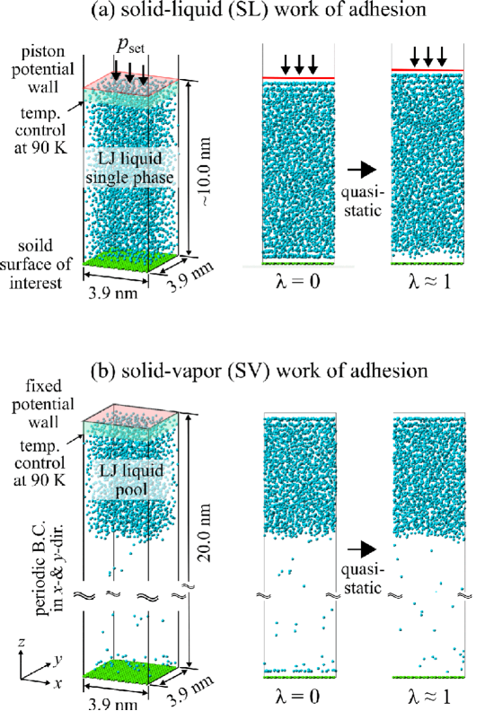
Figure 10: Simulation systems for the calculation of the solid-liquid and solid-vapor works of adhesion by the thermodynamic integration (TI) through the dry-surface (DS) scheme.

We calculated the solid-liquid (SL) and solid-vapor (SV) works of adhesion $W_{\mathrm{SL}}$ and $W_{\mathrm{SV}}$, respectively, by the thermodynamic integration (TI) Frenkel and Smit (1996) through the dry-surface (DS) scheme Leroy and Müller-Plathe (2015) to compare with the relative SL and SV interfacial tensions obtained in the present Wilhelmy MD systems. Details of the DS scheme were basically the same as in our previous study. Yamaguchi et al. (2019) In the systems shown in Fig. 10, the liquid or vapor was quasi-statically stripped off from the solid surface fixed on the bottom of the coordinate system, which had the same periodic honeycomb structure as the solid plate in the Wilhelmy MD system. The work of adhesion was calculated as the free energy difference after and before the above procedure, where the coupling parameter for the TI was embedded in the SF interaction parameter in the DS scheme.

For the calculation of $W_{\mathrm{SL}}$, a SL interface was formed between the liquid and bottom solid as shown in Fig. 10 (a) with wettability parameter $\eta$ corresponding to the Wilhelmy MD system. Periodic boundary condition was employed in the $x$-and $y$-directions tangential to the solid surface. In addition, we set a piston at $z=z_{\mathrm{pis}}$ above the liquid to attain a constant pressure system. By allocating sufficient number of fluid particles $N_{\mathrm{f}}$ and by setting the pressure $p_{\mathrm{set}}$ above the vapor pressure, a liquid bulk with a constant density was formed between the solid wall and piston. We used 3000 fluid particles, and the system size was set as shown in Fig. 10 (a). We also controlled the temperature of the fluid particles within 0.8 nm from the top piston regarding the velocity components in the $x$- and $y$-directions at $T_{\mathrm{c}}=90$ K.

We embedded a coupling parameter $\lambda$ into the SF interaction potential given in Eq. (5) as

$$\Phi^{\mathrm{DS}}_{\mathrm{sf}}(r_{ij},\lambda)=(1-\lambda)\Phi^{\mathrm{LJ}}_{\mathrm{sf}}(r_{ij}),$$ (59)

and we obtained multiple equilibrium systems with various $\lambda$ values with $0\leq\lambda<1$ to numerically calculate the TI described below. Each system was obtained after a preliminary equilibration of 10 ns, and the time average of 20 ns was used for the analysis.

The work of adhesion $W_{\mathrm{SL}}$ is defined by the minimum work needed to strip the liquid from the solid surface per area under constant $NpT$, and it can be calculated by the TI along a reversible path between the initial and final states of the process. In the present DS scheme, this was achieved by at first forming a SL interface, and then by weakening the SF interaction potential through the coupling parameter. We obtained equilibrium SL interfaces with discrete coupling parameter $\lambda$ varied from 0 to 0.999. Note that the maximum value of $\lambda$ was set slightly below 1 to keep the SF interaction to be effectively only repulsive. This value is denoted by $1^{-}$ hereafter. The difference of the SL interfacial Gibbs free energy $\Delta G_{\mathrm{SL}}\equiv G_{\mathrm{SL}}|_{\lambda=1^{-}}-G_{\mathrm{SL}}|_{\lambda=0}$ between systems at $\lambda=0$ and $\lambda=1^{-}$ under constant $NpT$ was related to the difference in the surface interfacial energies as

$$W_{\mathrm{SL}} \equiv \frac{\Delta G_{\mathrm{SL}}}{A}=\gamma_{\mathrm{S0}}+\gamma_{\mathrm{L0}}-\gamma_{\mathrm{SL}}$$ (60)

$$\approx \gamma_{\mathrm{S0}}+\gamma_{\mathrm{LV}}-\gamma_{\mathrm{SL}},$$

where the vacuum phase was denoted by subscript ‘0’ and $\gamma_{\mathrm{S0}}$ and $\gamma_{\mathrm{L0}}$ were the solid-vacuum and liquid-vacuum interfacial energies per unit area. Note that $\gamma_{\mathrm{L0}}$ was substituted by the liquid-vapor interfacial tension $\gamma_{\mathrm{LV}}$ in the final approximation considering that the vapor density was negligibly small. Using the $NpT$ canonical ensemble, the difference of the SL interfacial Gibbs free energy $\Delta G_{\mathrm{SL}}$ in Eq. (60) was calculated through the following TI:

$$\Delta G = \int_{0}^{1^{-}}\frac{dG(\lambda)}{d\lambda}d\lambda=\int_{0}^{1^{-}}\left<\frac{\partial H}{\partial\lambda}\right>d\lambda$$ (61)

$$= -\int_{0}^{1^{-}}\left<\sum_{i\in\mathrm{fluid}}^{N_{\mathrm{f}}}\sum_{j\in\mathrm{wall}}^{N_{\mathrm{w}}}\Phi_{\mathrm{fw}}\right>d\lambda,$$

$$\Delta G_{\mathrm{SL}}=\Delta G-Ap_{\mathrm{set}}\left(\left<z_{\mathrm{p}}|_{\lambda=1^{-}}\right>-\left<z_{\mathrm{p}}|_{\lambda=0}\right>\right)$$ (62)

where $H$ was the Hamiltonian, i.e., the internal energy of the system and $N_{\mathrm{w}}$ was the numbers of wall molecules. The ensemble average was substituted by the time average in the simulation, and was denoted by the angle brackets. Note that to obtain $\Delta G_{\mathrm{SL}}$, the work exerted on the piston $Ap_{\mathrm{set}}\left(\left<z_{\mathrm{p}}|_{\lambda=1^{-}}\right>-\left<z_{\mathrm{p}}|_{\lambda=0}\right>\right)$ was subtracted from the change of the Gibbs free energy of the system $\Delta G$ including the piston in Eq. (62).

For the calculation of the SV work of adhesion $W_{\mathrm{SV}}$, we investigated the interfacial energy between saturated vapor and corresponding solid surface set on the bottom of the simulation cell by placing an additional particle bath on the top as shown in Fig. 10 (b). The setup regarding the periodic boundary conditions employed in $x$-and $y$-directions, temperature control and placement conditions for the solid surface were the same as the SL system, whereas the particle bath was kept in place by a potential field at a fixed height sufficiently far from the solid surface. This potential field mimicked a completely wettable surface with an equilibrium contact angle of zero with the present potential parameters, i.e., a liquid film was formed on the particle bath. With this setting, a solid-vapor interface with the same density distribution as that in the Wilhelmy MD system was achieved. We formed multiple equilibrium systems with various values of the coupling parameter $\lambda$ with the same recipe as the SL systems.

Similar to the calculation of $W_{\mathrm{SL}}$, the SV interface at $\lambda=0$ was divided into S0 and V0 interfaces at $\lambda=1^{-}$ as shown in Fig. 10 (b), while the calculation systems for $W_{\mathrm{SV}}$ were under constant $NVT$. Thus, the solid-vapor work of adhesion $W_{\mathrm{SV}}$ was given by the difference of the Helmholtz free energy $\Delta F$ per unit area, and was related to the difference in the surface interfacial energy as

$$W_{\mathrm{SV}} \equiv \frac{\Delta{F}}{A}=\gamma_{\mathrm{S0}}+\gamma_{\mathrm{V0}}-\gamma_{\mathrm{SV}}$$ (63)

$$\approx \gamma_{\mathrm{S0}}-\gamma_{\mathrm{SV}},$$

where $\gamma_{\mathrm{V0}}$ was set zero in the final approximation. Using the $NVT$ canonical ensemble, $\Delta F$ in Eq. (63) was calculated through the TI as:

$$\Delta{F} = \int_{0}^{1^{-}}\frac{\partial F(\lambda)}{\partial\lambda}d\lambda=\int_{0}^{1^{-}}\left<\frac{\partial H}{\partial\lambda}\right>d\lambda$$ (64)

$$= -\int_{0}^{1^{-}}\left<\sum_{i}^{N_{\mathrm{f}}}\sum_{j}^{N_{\mathrm{w}}}\Phi^{\mathrm{LJ}}_{\mathrm{fw}}(r_{ij})\right>d\lambda.$$

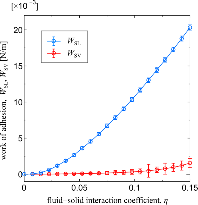
Figure 11: Works of adhesion $W_{\mathrm{SL}}$ and $W_{\mathrm{SV}}$ calculated by the TI as a function of the solid-fluid interaction coefficient $\eta$.

Figure 11 shows the SL and SV works of adhesion $W_{\mathrm{SL}}$ and $W_{\mathrm{SV}}$ calculated by the TI as a function of the solid-fluid interaction coefficient $\eta$. These values were used for the results shown in Fig. 8 through $\eta$-$\cos\theta$ relation in Fig. 9.

DATA AVAILABILITY

The data that support the findings of this study are available from the corresponding author upon reasonable request.

References

- de Gennes (1985) P.-G. de Gennes, ““Wetting” Statics and dynamics,” Rev. Mod. Phys. 57, 827–863 (1985).
- Ono and Kondo (1960) S. Ono and S. Kondo, Molecular Theory of Surface Tension in Liquids, Encyclopedia of Physics / Handbuch der Physik (Springer, 1960) pp. 134–280.
- Rowlinson and Widom (1982) J. S. Rowlinson and B. Widom, Molecular Theory of Capillarity (Dover, 1982).
- Schimmele, Naplórkowski, and Dietrich (2007) L. Schimmele, M. Naplórkowski, and S. Dietrich, “Conceptual aspects of line tensions,” J. Chem. Phys. 127 (2007), 10.1063/1.2799990, 0703821 [cond-mat] .
- Drelich et al. (2019) J. W. Drelich, L. Boinovich, E. Chibowski, C. D. Volpe, L. Hołysz, A. Marmur, and S. Siboni, “Contact angles: History of over 200 years of open questions,” Surf. Innov. , 1–25 (2019).
- Young (1805) T. Young, “An essay on the cohesion of fluids,” Phil. Trans. R. Soc. Lond. 95, 65 (1805).
- Gao and McCarthy (2009) L. Gao and T. J. McCarthy, “Wetting 101∘,” Langmuir 25, 14105–14115 (2009).
- Tanaka, Morigami, and Atoda (1993) T. Tanaka, M. Morigami, and N. Atoda, “Mechanism of resist pattern collapse during development process,” Jap. J. Appl. Phys. 32, 6059–6064 (1993).
- Kirkwood and Buff (1949) J. G. Kirkwood and F. P. Buff, “The statistical mechanical theory of surface tension,” J. Chem. Phys. 17, 338–343 (1949).
- Nijmeijer and van Leeuwen (1990) M. J. P. Nijmeijer and J. M. J. van Leeuwen, “Microscopic expressions for the surface and line tension,” J. Phys. A: Math. Gen. 23, 4211–4235 (1990).
- Nijmeijer et al. (1990) M. J. P. Nijmeijer, C. Bruin, A. F. Bakker, and J. M. J. van Leeuwen, “Wetting and drying of an inert wall by a fluid in a molecular-dynamics simulation,” Phys. Rev. A 42, 6052–6059 (1990).
- Tang and Harris (1995) J. Z. Tang and J. G. Harris, “Fluid wetting on molecularly rough surfaces,” J. Chem. Phys. 103, 8201–8208 (1995).
- Gloor et al. (2005) G. J. Gloor, G. Jackson, F. J. Blas, and E. De Miguel, “Test-area simulation method for the direct determination of the interfacial tension of systems with continuous or discontinuous potentials,” J. Chem. Phys. 123, 134703 (2005).
- Ingebrigtsen and Toxvaerd (2007) T. Ingebrigtsen and S. Toxvaerd, “Contact angles of Lennard-Jones liquids and droplets on planar surfaces,” J. Phys. Chem. C 111, 8518–8523 (2007).
- Das and Binder (2010) S. K. Das and K. Binder, “Does Young’s equation hold on the nanoscale? A Monte Carlo test for the binary Lennard-Jones fluid,” Europhy. Lett. 92, 26006 (2010).
- Weijs et al. (2011) J. H. Weijs, A. Marchand, B. Andreotti, D. Lohse, and J. H. Snoeijer, “Origin of line tension for a Lennard-Jones nanodroplet,” Phys. Fluids 23, 022001 (2011).
- Seveno, Blake, and de Coninck (2013) D. Seveno, T. D. Blake, and J. de Coninck, “Young’s equation at the nanoscale,” Phys. Rev. Lett. 111, 096101 (2013).
- Surblys et al. (2014) D. Surblys, Y. Yamaguchi, K. Kuroda, M. Kagawa, T. Nakajima, and H. Fujimura, “Molecular dynamics analysis on wetting and interfacial properties of water-alcohol mixture droplets on a solid surface,” J. Chem. Phys. 140, 034505 (2014).
- Nishida et al. (2014) S. Nishida, D. Surblys, Y. Yamaguchi, K. Kuroda, M. Kagawa, T. Nakajima, and H. Fujimura, “Molecular dynamics analysis of multiphase interfaces based on in situ extraction of the pressure distribution of a liquid droplet on a solid surface,” J. Chem. Phys. 140, 074707 (2014).
- Lau et al. (2015) G. V. Lau, I. J. Ford, P. A. Hunt, E. A. Müller, and G. Jackson, “Surface thermodynamics of planar, cylindrical, and spherical vapour-liquid interfaces of water,” J. Chem. Phys. 142, 114701 (2015).
- Yamaguchi et al. (2019) Y. Yamaguchi, H. Kusudo, D. Surblys, T. Omori, and G. Kikugawa, “Interpretation of Young’s equation for a liquid droplet on a flat and smooth solid surface: Mechanical and thermodynamic routes with a simple Lennard-Jones liquid,” J. Chem. Phys. 150, 044701 (2019).
- Kusudo, Omori, and Yamaguchi (2019) H. Kusudo, T. Omori, and Y. Yamaguchi, “Extraction of the equilibrium pinning force on a contact line exerted from a wettability boundary of a solid surface through the connection between mechanical and thermodynamic routes,” J. Chem. Phys. 151, 154501 (2019).
- Bey, Coasne, and Picard (2020) R. Bey, B. Coasne, and C. Picard, “Probing the concept of line tension down to the nanoscale,” J Chem. Phys. 152, 094707 (2020).
- Grzelak and Errington (2008) E. M. Grzelak and J. R. Errington, “Computation of interfacial properties via grand canonical transition matrix monte carlo simulation,” J. Chem. Phys. 128, 014710 (2008).
- Leroy, Dos Santos, and Müller-Plathe (2009) F. Leroy, D. J. V. A. Dos Santos, and F. Müller-Plathe, “Interfacial excess free energies of solid-liquid interfaces by molecular dynamics simulation and thermodynamic integration,” Macromol. Rapid Commun. 30, 864–870 (2009).
- Leroy and Müller-Plathe (2010) F. Leroy and F. Müller-Plathe, “Solid-liquid surface free energy of Lennard-Jones liquid on smooth and rough surfaces computed by molecular dynamics using the phantom-wall method,” J. Chem. Phys. 133, 044110 (2010).
- Kumar and Errington (2014) B. Kumar and J. R. Errington, “The use of monte carlo simulation to obtain the wetting properties of water,” Physics Procedia 53, 44–49 (2014).
- Leroy and Müller-Plathe (2015) F. Leroy and F. Müller-Plathe, “Dry-surface simulation method for the determination of the work of adhesion of solid–liquid interfaces,” Langmuir 31, 8335––8345 (2015).
- Ardham et al. (2015) V. R. Ardham, G. Deichmann, N. F. van der Vegt, and F. Leroy, “Solid-liquid work of adhesion of coarse-grained models of n-hexane on graphene layers derived from the conditional reversible work method,” J. Chem. Phys. 143, 243135 (2015).
- Kanduč and Netz (2017) M. Kanduč and R. R. Netz, “Atomistic simulations of wetting properties and water films on hydrophilic surfaces,” J Chem. Phys. 146, 164705 (2017).
- Kanduč (2017) M. Kanduč, “Going beyond the standard line tension: Size-dependent contact angles of water nanodroplets,” J. Chem. Phys. 147, 174701 (2017).
- Jiang, Müller-Plathe, and Panagiotopoulos (2017) H. Jiang, F. Müller-Plathe, and A. Z. Panagiotopoulos, “Going beyond the standard line tension: Size-dependent contact angles of water nanodroplets,” J. Chem. Phys. 147, 084708 (2017).
- Surblys et al. (2018) D. Surblys, F. Leroy, Y. Yamaguchi, and F. Müller-Plathe, “Molecular dynamics analysis of the influence of coulomb and van der waals interactions on the work of adhesion at the solid-liquid interface,” J. Chem. Phys. 148, 134707 (2018).
- Ravipati et al. (2018) S. Ravipati, B. Aymard, S. Kalliadasis, and A. Galindo, “On the equilibrium contact angle of sessile liquid drops from molecular dynamics simulations,” J. Chem. Phys. 148, 164704 (2018).
- Giacomello, Schimmele, and Dietrich (2016) A. Giacomello, L. Schimmele, and S. Dietrich, “Wetting hysteresis induced by nanodefects,” Proc. Natl. Acad. Sci. U. S. A. 113, E262–E271 (2016).
- Zhang, Müller-Plathe, and Leroy (2015) J. Zhang, F. Müller-Plathe, and F. Leroy, “Pinning of the contact line during evaporation on heterogeneous surfaces: Slowdown or temporary immobilization? insights from a nanoscale study,” Langmuir 31, 7544–7552 (2015).
- Zhang, Huang, and Lu (2019) J. Zhang, H. Huang, and X. Y. Lu, “Pinning-depinning mechanism of the contact line during evaporation of nanodroplets on heated heterogeneous surfaces: A molecular dynamics simulation,” Langmuir 35, 6356–6366 (2019).
- Wilhelmy (1863) L. Wilhelmy, “Ueber die Abhängigkeit der Capillaritäts-Constanten des Alkohols von Substanz und Gestalt des benetzten festen Körpers,” Ann. Phys. 195, 177–217 (1863), https://onlinelibrary.wiley.com/doi/pdf/10.1002/andp.18631950602 .
- Volpe and Siboni (2018) C. D. Volpe and S. Siboni, “The Wilhelmy method: a critical and practical review,” Surf. Innov. 6, 120–132 (2018).
- Marchand et al. (2012) A. Marchand, J. H. Weijs, J. H. Snoeijer, and B. Andreotti, “Why is surface tension a force parallel to the interface?” Am. J. Phys. 79, 999–1008 (2012).
- Das et al. (2011) S. Das, A. Marchand, B. Andreotti, and J. H. Snoeijer, “Elastic deformation due to tangential capillary forces,” Phys. Fluids 23, 1–11 (2011).
- Weijs, Andreotti, and Snoeijer (2013) J. H. Weijs, B. Andreotti, and J. H. Snoeijer, “Elasto-capillarity at the nanoscale: on the coupling between elasticity and surface energy in soft solids,” Soft Matter 9, 8494 (2013).
- Merchant and Keller (1992) G. J. Merchant and J. B. Keller, “Line tension between fluid phases and a substrate,” Phys. Fluids A 4, 477 (1992).
- Getta and Dietrich (1998) T. Getta and S. Dietrich, “Line tension between fluid phases and a substrate,” Phys. Rev. E 57, 655–671 (1998).
- Mastny and de Pablo (2007) E. A. Mastny and J. J. de Pablo, “Melting line of the Lennard-Jones system, infinite size, and full potential,” J. Chem. Phys. 127, 104504 (2007).
- Boruvka and Neumann (1977) L. Boruvka and A. W. Neumann, “Generalization of the classical theory of capillarity,” J. Chem. Phys. 66, 5464–5476 (1977).
- Marmur (1997) A. Marmur, “Line tension and the intrinsic contact angle in solid–liquid–fluid systems,” J. Colloid Interface Sci. 186, 462–466 (1997).
- Thompson et al. (1984) S. M. Thompson, K. E. Gubbins, J. P. R. B. Walton, R. A. R. Chantry, and J. S. Rowlinson, “A molecular dynamics study of liquid drops,” J. Chem. Phys. 81, 530–542 (1984).
- Yaguchi, Yano, and Fujikawa (2010) H. Yaguchi, T. Yano, and S. Fujikawa, “Molecular dynamics study of vapor-liquid equilibrium state of an argon nanodroplet and its vapor,” J. Fluid. Sci. Tech. 5, 180 (2010).
- Irving and Kirkwood (1950) J. H. Irving and J. G. Kirkwood, “The statistical mechanical theory of transport processes. IV. The equations of hydrodynamics,” J. Chem. Phys. 18, 817 (1950).
- Schofield and Henderson (1982) D. Schofield and J. R. Henderson, “Statistical mechanics of inhomogeneous fluids,” Proc. R. Soc. Lond. A 379, 231–246 (1982).
- Rowlinson (1993) J. S. Rowlinson, “Themodynamics of inhomogeneous systems,” Pure Appl. Chem. 65, 873–882 (1993).
- Frenkel and Smit (1996) D. Frenkel and B. Smit, Understanding Molecular Simulation: From Algorithms to Applications (Academic Press, 1996) pp. 152–156.