Tensor train rank minimization with nonlocal self-similarity for tensor completion

Abstract

The tensor train (TT) rank has received increasing attention in tensor completion due to its ability to capture the global correlation of high-order tensors ($\textrm{order}>3$). For third order visual data, direct TT rank minimization has not exploited the potential of TT rank for high-order tensors. The TT rank minimization accompany with ket augmentation, which transforms a lower-order tensor (e.g., visual data) into a higher-order tensor, suffers from serious block-artifacts. To tackle this issue, we suggest the TT rank minimization with nonlocal self-similarity for tensor completion by simultaneously exploring the spatial, temporal/spectral, and nonlocal redundancy in visual data. More precisely, the TT rank minimization is performed on a formed higher-order tensor called group by stacking similar cubes, which naturally and fully takes advantage of the ability of TT rank for high-order tensors. Moreover, the perturbation analysis for the TT low-rankness of each group is established. We develop the alternating direction method of multipliers tailored for the specific structure to solve the proposed model. Extensive experiments demonstrate that the proposed method is superior to several existing state-of-the-art methods in terms of both qualitative and quantitative measures.

Key words: low-rank tensor completion, tensor train rank, nonlocal self-similarity, alternating direction method of multipliers.

1 Introduction

Tensor completion aims at estimating missing entries or damaged parts in high-dimensional data and plays an important role in computer vision, e.g., color image inpainting [2, 29, 34, 54], video inpainting [6, 8, 52], hyperspectral images recovery [31, 48, 55], higher-order web link analysis [28, 35], and seismic data reconstruction [14]. As a typical ill-posed inverse problem, stable tensor completion processes usually rely on prior knowledge of the underlying tensor. Recently, the low-rankness prior has demonstrated to be a powerful tool for tensor completion, namely low-rank tensor completion (LRTC). A common way to characterize the low-rankness of tensors is to decompose them into several lower-dimensional multilinear spaces. Representative works on tensor rank include CANDECOMP/PARAFAC (CP) rank, Tucker rank [27], and tubal rank [26]; see Section 3 for a brief review on these related works.

Recently, the tensor train (TT) rank has achieved great success in LRTC. Given a $j$-th order tensor $\mathcal{X}\in\mathbb{R}^{n_{1}\times\cdots\times n_{j}}$, TT decomposition [40] models each element of $\mathcal{X}$ by

$$x_{i_{1},\ldots,i_{j}}=\mathcal{G}_{1}(:,i_{1},:)\cdots\mathcal{G}_{j}(:,i_{j},:),$$ (1)

where $\mathcal{G}_{k}\in\mathbb{R}^{r_{k-1}\times n_{k}\times r_{k}}$, $k=1,\cdots,j$ with $r_{0}=r_{j}=1$. The TT rank corresponding to (1) is defined as $(r_{1},\ldots,r_{j-1})$. The TT rank has shown to be effective in tensor completion due to its ability of capturing the intrinsic structure within higher-order tensors. Some optimization methods has been proposed for TT rank minimization, such as alternating minimization [18, 44], simple low-rank tensor completion via tensor train (SiLRTC-TT), and tensor completion by parallel matrix factorization via tensor train (TMac-TT) [1]; see Section 3 for more details.

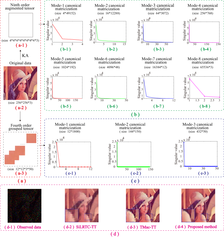
Figure 1: Comparison of TT low-rankness of higher-order tensors generated by KA and NSS. (a-1, 2, 3) the augmented tensor, the original data, and an example of grouped tensors. (b-1) to (b-8) the distribution of singular values of the mode-1 to mode-8 canonical matricizations of the augmented tensor (a-1) and the average ratio of singular values larger than $1\%$ of the corresponding largest ones is $25.8\%$. (c-1, 2, 3) the distribution of singular values of the mode-1, mode-2, and mode-3 canonical matricizations of the grouped tensor (a-3) and the average ratio of singular values larger than $1\%$ of the corresponding largest ones is $1.5\%$. (d-1, 2, 3, 4) the observed data, the recovered results by SiLRTC-TT, TMac-TT, and the proposed method.

Nevertheless, existing TT-based LRTC methods still leave much room for further improvement. Since most multidimensional visual data are of third order in practical applications, direct TT-rank minimization has not yet excavated the estimation potential of TT rank minimization. When handling third order visual data, such as color images and multispectral images, most existing methods use $ket\ augmentation$ (KA) [30] as a tensor order increment preprocessing to transform a lower-order tensor into a higher-order tensor. However, KA uses a fixed rule to stack blocks extracted from the original data, without considering the inherent correlation between different blocks, which leads to serious block-artifacts on restored images [11]; see Fig. 1 (d) for an example. To overcome this issue, our previous work [11] used the total variation regularizer to depict the spatial local smoothness prior of the underlying data. Although alleviating the block-artifacts to some extent, this method is still a palliative one, due to the ignorance of the intrinsic structural redundancy of real-world data. These motivate us to find a more adaptive method to retain the strength of TT rank and alleviate block-artifacts.

In this paper, we propose a novel scheme to adaptively generate higher-order tensors with TT low-rankness, by exploring the nonlocal self-similarity (NSS) prior of tensor data. As a significant intrinsic prior of natural images, NSS depicts the redundancy of repeated similar structures across a natural image, which has been demonstrated to be powerful in various image processing applications [7, 10, 19, 23, 38, 51]. Our main idea is to stack similar cubes into a higher-order tensor called a group. The motivation behind is that the similarity between cubes naturally implies the TT low-rankness of each group, which is more natural and effective than the fixed KA scheme. In fact, the perturbation analysis for the TT low-rankness of each group is established in Section 4. To explain our motivation, in Figure 1, we compare the TT low-rankness of two higher-order tensors generated by KA and NSS. We obtain two insights from Fig. 1. First, the canonical matricizations of the grouped higher-order tensor obtained by NSS exhibits low-rank property more significantly than that obtained by KA, which can be visually verified by the singular value curves shown in Fig. 1 (c-1, 2, 3) and Fig. 1 (b-1) to (b-8). Second, the proposed method can effectively alleviate block-artifacts compared with SiLRTC-TT and TMac-TT.

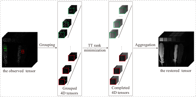
Figure 2: Flowchart of the proposed completion framework.

Once established, we develop a group-based TT rank minimization framework for tensor completion, which simultaneously exploits various data prior knowledge, such as spatial, temporal/spectral, and NSS redundancy. The main idea is to consider group as the basis unit of completion, and to impose the low-TT-rank constraint on each group to learn the correlations of all modes. Specifically, the proposed framework involves three steps. First, we stack $j$-th order similar cubes together into an $(j+1)$-th order tensor called a group and consider the group as the basis unit of completion. Second, we complete each group by solving a TT rank minimization model. Third, we calculate the final result by aggregating the final completed tensor by averaging all completed groups. The flowchart of the proposed method is illustrated in Fig. 2.

In summary, our contributions are mainly three folds: (1) we propose an adaptive strategy based on the NSS prior to fully exploit the potential of TT rank for high-order tensors, and establish a perturbation analysis for the TT low-rankness of groups consisting of similar cubes; (2) we propose a group-based TT rank minimization framework for tensor completion to simultaneously exploit the spatial, temporal/spectral, and NSS priors of tensor data; (3) experiments show that our method outperforms several state-of-the-art methods in handling multiple tensor completion problems.

The outline of this paper is as follows. Section 2 states some basic knowledge about tensors. Section 3 reviews some works about LRTC. Section 4 gives the details of the proposed method and establishes a perturbation analysis of the TT low-rankness of each group. Section 5 develops an alternating direction method of multipliers (ADMM)-based solving algorithm. Section 6 presents extensive numerical experiments. Section 7 discusses parameters study and the numerical convergence of the proposed algorithm. Section 8 summarizes this paper.

2 Preliminary

We denote scalars, vectors, matrices, and tensors as lowercase letters (e.g., $z$), boldface lowercase letters (e.g., z), boldface capital letters (e.g., Z), and calligraphic letters (e.g., $\mathcal{Z}$), respectively. A tensor is a high-dimensional array and its order (or mode) is the number of its dimensions. Given a $j$-th order tensor $\mathcal{Z}\in\mathbb{R}^{n_{1}\times\cdots\times n_{j}}$, its $(i_{1},\ldots,i_{j})$-th component is denoted as $z_{i_{1},\ldots,i_{j}}$. A mode-$k$ fiber of $\mathcal{Z}$ is a vector $\textbf{z}_{i_{1},\ldots,i_{k-1},:,i_{k+1},\ldots,i_{j}}$ obtained by varying index $i_{k}$ in while keeping the others fixed. The Frobenius norm of $\mathcal{Z}$ is $\|\mathcal{Z}\|_{F}=\sqrt{\langle\mathcal{Z},\mathcal{Z}\rangle}$, where $\langle\mathcal{X},\mathcal{Y}\rangle=\sum_{i_{1},\ldots,i_{j}}x_{i_{1},\ldots,i_{j}}\cdot y_{i_{1},\ldots,i_{j}}$ is the inner product of two tensors $\mathcal{X}$, $\mathcal{Y}$.

The mode-$k$ canonical matricization of $\mathcal{Z}$ is defined as $\textbf{Z}_{[k]}\in\mathbb{R}^{(\prod_{d=1}^{k}n_{d})\times(\prod_{d=k+1}^{j}n_{d})}$, where the element $(i_{1},\ldots,i_{j})$ of $\mathcal{Z}$ maps to the element $(a,b)$ of $\textbf{Z}_{[k]}$ satisfying

$$\begin{split}&a=1+\sum_{d=1}^{k}\big{(}(i_{d}-1)\prod_{t=1}^{d-1}n_{t}\big{)}\\ \textrm{and}\quad&b=1+\sum_{d=k+1}^{j}\big{(}(i_{d}-1)\prod_{t=k+1}^{d-1}n_{t}\big{)}.\end{split}$$ (2)

In MATLAB, it can be implemented by the reshape function

$$\textbf{Z}_{[k]}=\text{reshape}(\mathcal{Z},\Pi_{d=1}^{k}n_{d},\Pi_{d=k+1}^{j}n_{d}).$$

We denote the inverse operator as $\text{fold}_{[k]}(\textbf{Z}_{[k]})=\mathcal{Z}$. The TT nuclear norm of $\mathcal{Z}$ is defined as $\|\mathcal{Z}\|_{\ast}=\sum_{k=1}^{j-1}\alpha_{k}\|\textbf{Z}_{[k]}\|_{\ast}$, where $\{\alpha_{k}\}_{k=1}^{j-1}$ are positive constants satisfying $\sum_{k=1}^{j-1}\alpha_{k}=1$.

3 Related works

In this section, we briefly introduce some related works on the definition of tensor rank, including CP rank, Tucker rank [27], tubal rank [26], and TT rank [40].

The CP rank is defined as the smallest number of rank-one tensors that generate the target tensor. There exist some heuristic CP-based LRTC methods [35, 33, 41, 42, 50, 54], with promising performance. Nevertheless, computing CP rank is generally NP-hard [22], which limits its application. The Tucker rank is defined as a vector composed of ranks of unfolding matrices of the target tensor [27, 46]. Existing Tucker rank minimization methods include convex relaxation methods [12, 16, 32, 45] and low-rank matrix factorization methods [24, 49, 56]. The limitation of Tucker rank is that it only captures the correlation between one mode and all the rest modes of the tensor, due to the unbalanced matricization scheme in the unfolding operator [1]. The tensor tubal rank is defined as the number of nonzero singular tubes under the tensor singular value decomposition (tSVD) of the target tensor (please see [26, 36] for more details). Zhang et al. [53] proposed tensor nuclear norm (TNN) as a convex surrogate of tubal rank for LRTC. Moreover, Lu et al. [37] established the theoretical guarantee of TNN minimization for low tubal rank tensor recovery from Gaussian measurements.

For TT rank, according to [40], there exists decomposition that makes $r_{k}$ equal to the rank of the canonical matrix $X_{[k]}\in\mathbb{R}^{(\prod_{d=1}^{k}n_{d})\times(\prod_{d=k+1}^{j}n_{d})}$, a well-balanced matricization characterizing the correlation between the first $k$ and the rest $j-k$ dimensions of $\mathcal{X}$ [1]. Compared with existing works, the TT decomposition and TT rank have two significant advantages. First, the TT decomposition is free from the “curse of dimensionality” [40], which enables its applications to large-scale problems. Second, the TT rank, approximately calculated by the rank of canonical matrices, can capture the global correlation of higher-order tensors due to its well-balanced matricization scheme, i.e., matricizing the tensor along permutations of modes.

Researchers have developed a series of methods for TT rank minimization. Grasedyck et al. [18] and Wang et al. [44] proposed an iterative algorithm by alternatively updating each core tensor. However, [18] fixed the TT rank as $r_{1}=\cdots=r_{j-1}$, and [44] assumed that the TT rank is given. Recently, Bengua et al. [1] proposed two TT minimization models for LRTC. The first one, simple low-rank tensor completion via tensor train (SiLRTC-TT), minimizes the sum of nuclear norm of canonical matrices, i.e.,

$$\begin{split}\min_{\mathcal{X}}\quad&\sum_{k=1}^{j-1}\alpha_{k}\|\textbf{X}_{[k]}\|_{\ast}\\ s.t.\quad&\mathcal{P}_{\Omega}(\mathcal{X})=\mathcal{P}_{\Omega}(\mathcal{T}),\end{split}$$ (3)

where $\textbf{X}_{[k]}$ is the mode-$k$ canonical matricization of the tensor $\mathcal{X}$ and $\{\alpha_{k}\}_{k=1}^{j-1}$ are positive constants satisfying $\sum_{k=1}^{j-1}\alpha_{k}=1$, $\mathcal{T}\in\mathbb{R}^{n_{1}\times\ldots\times n_{j}}$ is the observed tensor, $\Omega$ is the index of observed entries, and $\mathcal{P}_{\Omega}(\cdot)$ is the projection operator that keeps entries in $\Omega$ and zeros out others. Another one, tensor completion by parallel matrix factorization via tensor train (TMac-TT), uses matrix factorization to approximate the TT rank, i.e.,

$$\begin{split}\min_{\{\textbf{W}_{k}\}_{k=1}^{j-1},\{\textbf{Z}_{k}\}_{k=1}^{j-1},\mathcal{X}}\quad&\sum_{k=1}^{j-1}\frac{\alpha_{k}}{2}\|\textbf{W}_{k}\textbf{Z}_{k}-\textbf{X}_{[k]}\|_{F}^{2}\\ s.t.\quad&\mathcal{P}_{\Omega}(\mathcal{X})=\mathcal{P}_{\Omega}(\mathcal{T}),\end{split}$$ (4)

where $\textbf{W}_{k}\in\mathbb{R}^{(\prod_{d=1}^{k}n_{d})\times r_{k}}$, $\textbf{Z}_{k}\in\mathbb{R}^{r_{k}\times(\prod_{d=k+1}^{j}n_{d})}$, and $r_{k}$ is the rank of the matrix $\textbf{X}_{[k]}$.

4 Tensor completion via nonlocal TT rank minimization

The proposed method, called tensor completion via nonlocal TT rank minimization (NL-TT), involves three main steps: grouping, completion, and aggregation. Below we detail each step.

Grouping. We use a third order tensor $\mathcal{T}\in\mathbb{R}^{n_{1}\times n_{2}\times n_{3}}$ as an example to show how to construct groups, which can be easily extended to higher-order tensors. We extract reference cubes with size $s\times s\times n_{3}$ with overlapped size $o$, denoted as $\{\mathcal{\hat{T}}_{p}\}_{p=1}^{t}$, where the total number of reference cubes is $t=((n_{1}-s)/(s-o)+1)\times((n_{2}-s)/(s-o)+1)$. We use block-matching [10] to find the locations of similar cubes and adopt the Euclidean distance to measure the similarity between two cubes. A smaller distance indicates a higher similarity. For each reference cube $\mathcal{\hat{T}}_{p}$, we assume that $h$ cubes $\{\mathcal{\hat{T}}_{p}^{a}\}$ ($a=1,2,\ldots,h$) similar to $\mathcal{\hat{T}}_{p}$ are found in spatial domain. These cubes are chosen to overlap to avoid possible block effects. Then we stack the similar cubes to form a group $\mathcal{T}_{p}\in\mathbb{R}^{s\times s\times n_{3}\times h}$ satisfying $\mathcal{T}_{p}(:,:,:,a)=\mathcal{\hat{T}}_{p}^{a}$.

Completion. Let $\mathcal{T}_{p}$ be a $j$-th order grouped tensor, and $\Omega_{p}$ be the indicating known pixels of $\mathcal{T}_{p}$. To complete $\mathcal{T}_{p}$, we consider the following TT nuclear norm minimization model:

$$\begin{split}\min_{\mathcal{X}_{p}}\quad&\|\mathcal{X}_{p}\|_{*}:=\sum_{k=1}^{j-1}\alpha_{k}\|\textbf{X}_{p,[k]}\|_{\ast}\\ s.t.\quad&\mathcal{P}_{\Omega_{p}}(\mathcal{X}_{p})=\mathcal{P}_{\Omega_{p}}(\mathcal{T}_{p}),\end{split}$$ (5)

where $\textbf{X}_{p,[k]}$ is the mode-$k$ canonical matricization of the tensor $\mathcal{X}_{p}$ and $\{\alpha_{k}\}_{k=1}^{j-1}$ are positive constants satisfying $\sum_{k=1}^{j-1}\alpha_{k}=1$. The following proposition shows the existence of the solution of the proposed model (5).

Proposition 1.

The model (5) has at least one minimizer.

The proof is provided in Appendix A.

Aggregation. After completing each group, the obtained estimates actually form an over-complete representation of the final completion result. Since the cubes are overlapped and one cube can appear in more than one group, each pixel may be covered by several completed groups. The final completion result is calculated by first returning completed groups to their original positions and then averaging all covered cubes pixel-by-pixel.

4.1 Perturbation analysis

We establish a perturbation analysis for the TT low-rankness of the group consisting of similar cubes. Assume that $\mathcal{X}$ is a group with size $s\times s\times n_{3}\times h$. Next, we first show that $\mathcal{X}$ can be approximated by a series of TT low-rank tensors. Then, we present a perturbation analysis of the TT nuclear norm of $\mathcal{X}$ and its TT low-rank approximations.

Now we can establish an upper bound between $\mathcal{X}$ and a TT rank-$(1,1,1)$ tensor.

Theorem 1.

Let $\mathbf{x}$ be the average column fiber of $\mathcal{X}$, i.e., $\mathbf{x}=(\sum_{i_{2}=1}^{s}\sum_{i_{3}=1}^{n_{3}}\sum_{i_{4}=1}^{h}\mathcal{X}(:,i_{2},i_{3},i_{4}))/(sn_{3}h)$, and $\mathcal{Y}(:,i_{2},i_{3},i_{4})=\mathbf{x},i_{2}=1,\ldots,s,i_{3}=1,\ldots,n_{3}$, and $i_{4}=1,\ldots,h$. Then the TT rank of $\mathcal{Y}$ is $(1,1,1)$. Suppose that

$$\max_{i_{2},i_{3},i_{4}}\{\|\mathcal{X}(:,i_{2},i_{3},i_{4})-\mathbf{x}\|_{2}\}\leq\varepsilon.$$

Let $\mathcal{X}=\mathcal{Y}+\mathcal{E}$. Then $\|\mathcal{E}\|_{F}\leq\sqrt{sn_{3}h}\varepsilon$.

We consider the TT rank-$(r_{1},r_{2},1)$ approximation of $\mathcal{X}$.

Theorem 2.

Let $\mathcal{\hat{X}}$ be the average row-cube of $\mathcal{X}$, i.e., $\mathcal{\hat{X}}=(\sum_{i_{4}=1}^{h}\mathcal{X}(:,:,:,i_{4}))/h$, and $\mathcal{Y}(:,:,:,i_{4})=\mathcal{\hat{X}},i_{4}=1,\ldots,h$. Then, $\mathcal{Y}$ is a TT rank-$(r_{1},r_{2},1)$ tensor, $r_{1}\leq\min\{s,sn_{3}h\}$, and $r_{2}\leq\min\{s^{2},n_{3}h\}$. Suppose that

$$\max_{i_{4}}\{\|\mathcal{X}(:,:,:,i_{4})-\mathcal{\hat{X}}\|_{F}\}\leq\hat{\varepsilon}.$$

Let $\mathcal{X}=\hat{\mathcal{Y}}+\hat{\mathcal{E}}$. Then $\|\hat{\mathcal{E}}\|_{F}\leq\sqrt{h}\hat{\varepsilon}$.

Next, we consider the TT rank-$(\tilde{r}_{1},\tilde{r}_{2},r)$ approximation of $\mathcal{X}$. Let $\mathcal{R}:=\{1,2,\ldots,r\}$.

Theorem 3.

Let $\mathcal{X}=\mathcal{\tilde{Y}}+\mathcal{\tilde{E}}$, where $\mathcal{\tilde{Y}}(:,:,:,a)=\mathcal{X}(:,:,:,a),a=1,\ldots,r$, $\mathcal{\tilde{Y}}(:,:,:,a)=\mathcal{X}(:,:,:,1),a=r+1,\ldots,h$, i.e., $\mathcal{\tilde{Y}}=[\mathcal{X}(:,:,:,1),\mathcal{X}(:,:,:,2),\ldots,\mathcal{X}(:,:,:,r),\mathcal{X}(:,:,:,1),\ldots,\mathcal{X}(:,:,:,1)]\in\mathbb{R}^{s\times s\times n_{3}\times h}$. The TT rank of $\mathcal{Y}$ is $(\tilde{r}_{1},\tilde{r}_{2},r)$. Suppose that $\{\|\mathcal{X}(:,:,:,b)-\mathcal{X}(:,:,:,i_{4})\|_{F}\}\leq\tilde{\varepsilon}$ for $b\in\mathcal{R}$ and $i_{4}=1,\ldots,h$. Then

$$\|\mathcal{\tilde{E}}\|_{F}\leq\sqrt{h-r}\tilde{\varepsilon}.$$

Last, we display a perturbation analysis of the TT nuclear norm of $\mathcal{X}$ using the following lemma.

Lemma 1.

(Corollary 4.31, [43]) Let $\textbf{X},\textbf{E}\in\mathbb{C}^{m\times n}(m\geq n)$. Then

$$|\sigma_{i}(\textbf{X}+\textbf{E})-\sigma_{i}(\textbf{X})|\leq\|\textbf{E}\|_{F},$$

where $\sigma_{i}(\textbf{X})$ is the $i$-th largest singular value, $i=1,\ldots,n$.

Theorem 4.

Let $\mathcal{X}=\mathcal{Y}+\mathcal{E}$, $s(\mathcal{X})=\sum_{k=1}^{3}\alpha_{k}\|\textbf{X}_{[k]}\|_{\ast}$, where $\|\textbf{X}_{[k]}\|_{\ast}=\sum_{j_{k}}\sigma_{j_{k}}(\textbf{X}_{[k]})$ and $\{\alpha_{k}\}_{k=1}^{3}$ are positive constants satisfying $\sum_{k=1}^{3}\alpha_{k}=1$. Then

$$|s(\mathcal{X})-s(\mathcal{Y})|\leq c\|\mathcal{E}\|_{F},$$

where $c$ is a positive constant.

The proofs are provided in Appendix B.

Remark 1.

We can regard the stacked higher-order tensor as a TT low-rank tensor plus a perturbation noisy tensor. In this case, Theorems 1, 2, and 3 show that $\mathcal{X}$ can be approximated by the TT rank-$(1,1,1)$, rank-$(r_{1},r_{2},1)$, and rank-$(\tilde{r}_{1},\tilde{r}_{2},r)$ tensors, respectively. Theorem 4 illustrates that the singular values are insensitive to the perturbation in the tensor. When $\mathcal{Y}$ is a TT low-rank tensor and $\mathcal{E}$ is small, the stacked higher-order tensor approximates a TT low-rank tensor.

The above results can be easily extended to higher-order tensors.

5 The ADMM solver

We develop ADMM [5, 17, 39] to solve the convex optimization problem (5). By introducing auxiliary variables $\{\mathcal{M}_{k}\}_{k=1}^{j-1}$, we obtain the equivalent constrained problem

$$\begin{split}\mathop{\mathrm{arg\,min}}_{\mathcal{X},\mathcal{M}_{k}}&\ \sum_{k=1}^{j-1}\alpha_{k}\|\mathcal{M}_{k[k]}\|_{*}\\ s.t.&\ \mathcal{P}_{\Omega}(\mathcal{X})=\mathcal{P}_{\Omega}(\mathcal{T}),\\ &\ \mathcal{X}=\mathcal{M}_{k},k=1,\ldots,j-1.\end{split}$$ (6)

The augmented Lagrangian function of (6) is defined as

$$\begin{split}\mathcal{L}_{\beta}(\mathcal{X},\mathcal{M}_{k},\mathcal{Y}_{k})=\sum_{k=1}^{j-1}\alpha_{k}&\Big{(}\|\mathcal{M}_{k[k]}\|_{*}+\langle\mathcal{X}-\mathcal{M}_{k},\mathcal{Y}_{k}\rangle\\ &+\frac{\beta}{2}\|\mathcal{X}-\mathcal{M}_{k}\|_{F}^{2}\Big{)},\end{split}$$ (7)

where $\{\mathcal{Y}_{k}\}_{k=1}^{j-1}$ are Lagrangian multipliers of the linear constraint and $\beta$ is the penalty parameter. We use the following iterative scheme to solve (7):

$$\left\{\begin{array}[]{l}\begin{split}\vspace{0.1cm}&\mathcal{M}_{k}^{l+1}=\mathop{\mathrm{arg\,min}}_{\mathcal{M}_{k}}\mathcal{L}(\mathcal{X}^{l},\mathcal{M}_{k},\mathcal{Y}_{k}^{l}),\\ \vspace{0.2cm}&\mathcal{X}^{l+1}=\mathop{\mathrm{arg\,min}}_{\mathcal{P}_{\Omega}(\mathcal{X})=\mathcal{P}_{\Omega}(\mathcal{T})}\mathcal{L}(\mathcal{X},\mathcal{M}_{k}^{l+1},\mathcal{Y}_{k}^{l}),\\ \vspace{0.1cm}&\mathcal{Y}_{k}^{l+1}=\mathcal{Y}_{k}^{l}+\beta(\mathcal{X}^{l+1}-\mathcal{M}_{k}^{l+1}).\\ \end{split}\end{array}\right.$$ (8)

We give the details for solving the first two subproblems in (8).

(1) $\{\mathcal{M}_{k}\}$-subproblem.  The optimal $\mathcal{M}_{k}$ is given by

$$\mathcal{M}_{k}^{l+1}=\mathop{\mathrm{arg\,min}}_{\mathcal{M}_{k}}\|\mathcal{M}_{k[k]}\|_{*}+\frac{\beta}{2}\|\mathcal{X}^{l+1}-\mathcal{M}_{k}+\frac{\mathcal{Y}_{k}^{l}}{\beta}\|_{F}^{2}.$$ (9)

Using the equation $\|\textbf{X}_{[k]}\|_{F}=\|\mathcal{X}\|_{F}$, we rewrite the (9) as the following problem:

$$\mathcal{M}_{k}^{l+1}=\mathop{\mathrm{arg\,min}}_{\mathcal{M}_{k}}\|\mathcal{M}_{k[k]}\|_{*}+\frac{\beta}{2}\|\mathcal{X}^{l+1}_{[k]}-\mathcal{M}_{k[k]}+\frac{\mathcal{Y}_{k[k]}^{l}}{\beta}\|_{F}^{2}.$$ (10)

Using the singular value thresholding operator [4], $\mathcal{M}_{k}$ has the closed-form solution

$$\mathcal{M}_{k}^{l+1}=\textrm{fold}_{[k]}\big{[}\textbf{U}_{k}S_{\frac{1}{\beta}}(\Sigma_{k})\textbf{V}_{k}^{T}\big{]},$$ (11)

where $\mathcal{X}^{l+1}_{[k]}+\frac{\mathcal{Y}_{k[k]}^{l}}{\beta}=\textbf{U}_{k}\Sigma_{k}\textbf{V}_{k}^{T}$ and $S_{\frac{1}{\beta}}(\Sigma_{k})=\textrm{diag}(\textrm{max}(\sigma_{k}-\frac{1}{\beta}))$. The $\mathcal{M}_{k}$-subproblem involves the SVD of the matrix $\mathcal{M}_{k[k]}$ with size $p_{k}\times q_{k}$ ($p_{k}=\prod_{d=1}^{k}n_{d},\ q_{k}=\prod_{d=k+1}^{j}n_{d},\ k=1,\ldots,j-1$), whose complexity is $O\big{(}\textrm{min}\big{(}p_{k}^{2}q_{k},\ p_{k}q_{k}^{2}\big{)}\big{)}$.

(2) $\mathcal{X}$-subproblem.  The optimal $\mathcal{X}$ is the solution of the following quadratic problem:

$$\mathcal{X}^{l+1}=\mathop{\mathrm{arg\,min}}_{\mathcal{P}_{\Omega}(\mathcal{X})=\mathcal{P}_{\Omega}(\mathcal{T})}\sum_{k=1}^{j-1}\frac{\alpha_{k}\beta}{2}\|\mathcal{X}-\mathcal{M}_{k}^{l}+\frac{\mathcal{Y}_{k}^{l}}{\beta}\|_{F}^{2}.$$ (12)

Then $\mathcal{X}$ can be calculated by

$$\mathcal{X}^{l+1}=\mathcal{P}_{\Omega^{c}}\Bigg{(}\sum_{k=1}^{j-1}\alpha_{k}\Big{(}\mathcal{M}_{k}-\frac{1}{\beta}\mathcal{Y}_{k}\Big{)}\Bigg{)}+\mathcal{P}_{\Omega}(\mathcal{T}).$$ (13)

The cost of computing $\mathcal{X}$ is $O(\prod_{k=1}^{j}n_{k})$.

The proposed ADMM-based algorithm is summarized in Algorithm 1. The minimization problem (6) fits the framework of ADMM, and the proposed model is convex, thus the proposed algorithm is theoretically convergent [13, 20]. At each iteration, the total cost of computing all variables is

$$O\bigg{(}t\sum_{k=1}^{j-1}\textrm{min}\big{(}p_{k}^{2}q_{k},\ p_{k}q_{k}^{2}\big{)}\bigg{)},$$

where $t$ is the number of reference cubes, $p_{k}=\prod_{d=1}^{k}n_{d}$, and $q_{k}=\prod_{d=k+1}^{j}n_{d},\ k=1,\ldots,j-1.$

Algorithm 1 ADMM-based algorithm for solving (5).

1:The observed tensor $\mathcal{T}$, index set $\Omega$.

2:Grouping: Perform block-matching to get $\{\mathcal{T}_{p}\}_{p=1}^{t}$.

3:Out loop: For $p=1,\cdots,t$, do

4: Parameters: $\{\alpha_{k}\}_{k=1}^{j-1}$, $\beta$, and inner iteration $l_{max}$.

5: Initialize: $\mathcal{X}^{0}_{p}=\mathcal{T}_{p}$ and $\mathcal{Y}^{0}_{p,k}=0$.

6: Inner loop: While $l\leq l_{max}$ or $\frac{\|\mathcal{X}^{l+1}_{p}-\mathcal{X}^{l}_{p}\|_{F}}{\|\mathcal{X}^{l}_{p}\|_{F}}\geq 10^{-4}$, do

7:   for $k=1$ to $j-1$ do;

8:     update $\mathcal{M}_{k}$ via (11);

9:   end for;

10:   update $\mathcal{X}_{p}$ via (13);

11: end while, and output $\mathcal{X}_{p}^{l+1}$.

12:end for, and output completed $\{\mathcal{X}_{p}\}_{p=1}^{t}$.

13:Recovered data $\mathcal{X}$ via completed groups $\{\mathcal{X}_{p}\}_{p=1}^{t}$.

(a) peppers	(b) lena	(c) house	(d) barbara
(e) facade	(f) airplane	(g) monarch	(h) sailboat

Figure 3: Original images.

6 Experiments

In this section, we evaluate the performance of the proposed method by extensive experiments on color images, multispectral images (MSIs), and color videos. We compare our method (NL-TT) with four well-known methods: HaLRTC [32], tSVD [53], SiLRTC-TT, and TMac-TT [1]. The range of entry values for all test tensors are scaled into the interval $[0,255]$. In color videos tests, as tSVD is only applicable to third order tensors, we perform it on each frame separately. All numerical experiments are performed on Windows 10 64-bit and MATLAB R2012a running on a desktop equipped with an Intel(R) Core(TM) i7-6700M CPU with 3.40 GHz and 8 GB of RAM.

We use the peak signal-to-noise ratio (PSNR) and the structural similarity index (SSIM) to evaluate the quality of restored results. PSNR (dB) and SSIM measure the similarity between the original tensor and the recovered tensor based on the distance and structural consistency, respectively. By calculating average PSNR and SSIM values for all bands, we obtain the PSNR and SSIM values of a higher-order tensor. Higher PSNR and SSIM values indicate better image quality.

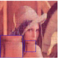
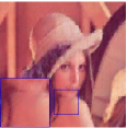
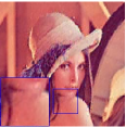
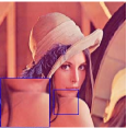
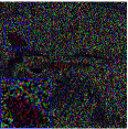
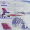
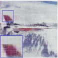
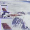
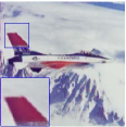
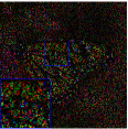
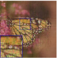
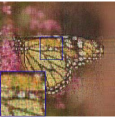
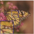
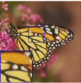
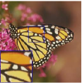
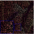
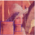
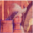
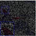
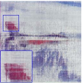
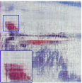
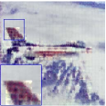
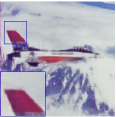
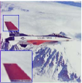
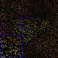
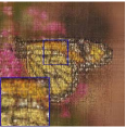
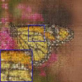
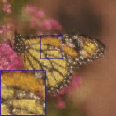
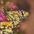
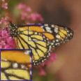
(a) Observed	(b) HaLRTC	(c) tSVD	(d) SiLRTC-TT	(e) TMac-TT	(f) NL-TT	(g) Original

Figure 4: The results of testing color images with $SR=0.2$ recovered by different methods. The first three rows and second three rows represent random sampling and tube sampling, respectively. From left to right: (a) the observed image, the results by (b) HaLRTC, (c) tSVD, (d) SiLRTC-TT, (e) TMac-TT, (f) NL-TT, and (g) the original image.

Parameters setting. In the block-matching operator, there are three important parameters: the cube size, the similar cube number, and the overlapping cube size. We set the cube size $s\in[10,20]$ with the increment 2, the number of similar cubes $h\in[30,50]$ with the increment 4, and the overlapping cube size as $o=1$. In our model (5), we assign larger weights to $\textbf{X}_{p,[k]}$ with balanced sizes, i.e.,

$$\small\alpha_{k}=\frac{\delta_{k}}{\sum_{k=1}^{j-1}\delta_{k}}\quad\text{with}\quad\delta_{k}=\min(\Pi_{d=1}^{k}n_{d},\Pi_{d=k+1}^{j}n_{d}),$$ (14)

where $n_{d}$ is the $d$-th order of $\mathcal{X}_{p}$ and $k=1,\ldots,j-1$. In the ADMM solver, we empirically select the penalty parameter $\beta$ in (7) from the candidate set:  {0.05, 0.08, 0.1, 0.3, 0.5}, to attain the highest PSNR value. For each completed groups, we stop the proposed algorithm according to the relative error of the tensor $\mathcal{X}_{p}$ between two successive iterations as follows:

$$\small\frac{\|\mathcal{X}^{l+1}_{p}-\mathcal{X}^{l}_{p}\|_{F}}{\|\mathcal{X}^{l}_{p}\|_{F}}\leq 10^{-4}.$$ (15)

In addition, we set the maximum inner iterations $l_{max}=500$. We try our best to tune the parameters involved in the competing algorithms according to the reference papers’ suggestion.

Table 1: The PSNR and SSIM values obtained by HaLRTC, tSVD, SiLRTC-TT, TMac-TT and NL-TT for color image data with different sampling rates (SRs). The first three rows and second three rows represent random sampling and tube sampling, respectively.

Image	SR	0.1		0.2		0.3		0.4
	Method	PSNR	SSIM	PSNR	SSIM	PSNR	SSIM	PSNR	SSIM
lena	HaLRTC	19.29	0.4151	23.10	0.6047	25.68	0.7311	28.00	0.8205
	tSVD	19.55	0.3500	23.33	0.5572	26.08	0.7033	28.60	0.8066
	SiLRTC-TT	21.67	0.5954	24.80	0.7366	27.01	0.8226	28.90	0.8782
	TMac-TT	24.25	0.6829	27.22	0.8097	28.87	0.8584	30.22	0.8902
	NL-TT	26.46	0.8110	30.09	0.8970	32.02	0.9309	33.87	0.9528
airplane	HaLRTC	19.80	0.4621	23.18	0.6437	25.62	0.7614	27.97	0.8399
	tSVD	19.87	0.4196	23.30	0.6139	25.86	0.7387	28.25	0.8258
	SiLRTC-TT	20.81	0.6072	23.42	0.7361	25.62	0.8213	27.55	0.8768
	TMac-TT	22.46	0.6766	25.81	0.8105	27.67	0.8622	28.97	0.8915
	NL-TT	24.33	0.7840	28.33	0.8929	30.29	0.9268	31.99	0.9489
monarch	HaLRTC	17.12	0.4381	19.59	0.6069	21.89	0.7404	24.20	0.8271
	tSVD	17.14	0.3372	19.98	0.5462	22.60	0.6980	25.23	0.8023
	SiLRTC-TT	17.95	0.5784	20.32	0.7196	22.38	0.8100	24.39	0.8702
	TMac-TT	19.21	0.6621	22.45	0.7912	24.86	0.8505	27.24	0.9046
	NL-TT	22.22	0.8307	25.42	0.9140	27.95	0.9496	30.74	0.9729
lena	HaLRTC	17.54	0.2942	20.97	0.4651	23.59	0.6144	25.88	0.7272
	tSVD	17.88	0.2570	20.85	0.4186	23.29	0.5676	25.50	0.6857
	SiLRTC-TT	20.90	0.5462	23.61	0.6830	25.69	0.7732	27.35	0.8353
	TMac-TT	21.62	0.5629	24.60	0.7193	26.22	0.7764	27.55	0.8392
	NL-TT	23.94	0.7351	27.45	0.8459	29.33	0.8928	31.38	0.9259
airplane	HaLRTC	17.81	0.3050	20.77	0.4847	23.15	0.6214	25.29	0.7289
	tSVD	17.97	0.2900	20.66	0.4588	22.97	0.5926	25.06	0.7029
	SiLRTC-TT	20.20	0.5570	22.49	0.6809	24.33	0.7661	26.09	0.8298
	TMac-TT	21.06	0.6169	23.15	0.7114	24.41	0.7729	26.17	0.8416
	NL-TT	22.45	0.7255	25.25	0.8210	27.29	0.8749	29.24	0.9149
monarch	HaLRTC	16.04	0.3424	18.28	0.5031	20.12	0.6363	21.93	0.7401
	tSVD	16.33	0.2786	18.21	0.4312	19.90	0.5620	21.65	0.6791
	SiLRTC-TT	17.46	0.5472	19.48	0.6695	21.19	0.7606	22.83	0.8290
	TMac-TT	15.12	0.3466	18.66	0.6710	21.74	0.7739	23.49	0.8282
	NL-TT	18.07	0.6564	22.33	0.8462	24.53	0.9086	26.25	0.9391

6.1 Color images

We evaluate the performance of NL-TT on color images. The test images of size $256\times 256\times 3$ are shown in Fig. 3. For color images, we test two kinds of missing entries: (1) random missing entries, including random sampling and tube sampling; and (2) structural missing entries, including missing curves, missing slices, missing texts, and missing blocks. The sampling rate (SR) is tested from 0.05 to 0.6.

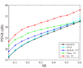
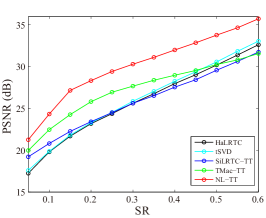
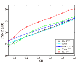
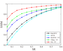
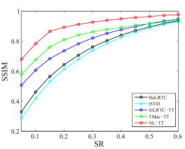
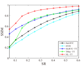
(a) lena	(b) airplane	(c) monarch

Figure 5: The PSNR and SSIM values of the reconstructed color image results for random missing entries by different methods.

Random sampling and tube sampling. The random sampling denotes that the entries in R, G, and B channels are randomly and independently lost in the color image, see the first three rows in Fig. 4 (a). The tube sampling means that the entries are randomly lost at the same location in R, G, and B channels, see the second three rows in Fig. 4 (a). The task for recovering the tube sampling is harder than the random sampling. Fig. 4 shows the visually restored results recovered by HaLRTC, tSVD, SiLRTC-TT, TMac-TT, and NL-TT. The first three lines are random sampling with $SR=0.2$. The second three lines are tube sampling with $SR=0.2$. We observe that the results recovered by both HaLRTC and tSVD have undesired thorns. Although SiLRTC-TT and TMac-TT obtain much better results than HaLRTC and tSVD, some block-artifacts are created on the restored images. As a comparison, the recovered results by the proposed method are visually better than those of the compared methods. From the zoom-in regions of recovered images, we observe that NL-TT can efficiently keep the details and smoothness of images and reduce the block-artifacts compared with SiLRTC-TT and TMac-TT.

Table 1 lists the PSNR and SSIM values of the restored images by all compared methods on different SRs. The highest results for each quality index are labeled in bold. Fig. 5 shows the recovery PSNR and SSIM curves by all compared methods with SRs tested from 0.05 to 0.6. It is observed that for different SRs, the proposed method achieves the highest PSNR and SSIM values.

Structural missing pixels. We test five kinds of structural missing pixels, i.e., missing random curves for image house, missing random vertical and horizontal slices for image facade, missing texts for image sailboat, and missing regular and random blacks for images barbara and peppers, respectively.

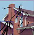
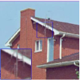
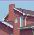
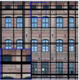
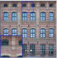
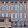
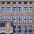
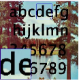
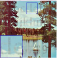
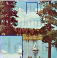
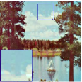
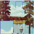
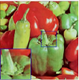
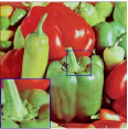
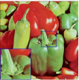
(a) Observed	(b) HaLRTC	(c) tSVD	(d) SiLRTC-TT	(e) TMac-TT	(f) NL-TT	(g) Original

Figure 6: The results of testing color images with structural missing entries recovered by different methods. From left to right: (a) the observed image, the results by (b) HaLRTC, (c) tSVD, (d) SiLRTC-TT, (e) TMac-TT, (f) NL-TT, and (g) the original image.

Table 2: The PSNR and SSIM values obtained by HaLRTC, tSVD, SiLRTC-TT, TMac-TT and NL-TT for color image data with structural missing entries.

Method	HaLRTC		tSVD		SiLRTC-TT		TMac-TT		NL-TT
Image	PSNR	SSIM	PSNR	SSIM	PSNR	SSIM	PSNR	SSIM	PSNR	SSIM
house	36.44	0.9707	36.14	0.9681	38.52	0.9793	38.03	0.9740	45.34	0.9906
facade	12.95	0.5681	12.95	0.5681	28.14	0.9062	27.50	0.8947	29.60	0.9357
sailboat	26.49	0.8700	26.69	0.8696	26.53	0.8838	26.40	0.8995	27.86	0.9370
barbara	32.44	0.9580	32.44	0.9579	33.99	0.9681	33.29	0.9654	37.56	0.9867
peppers	31.64	0.9595	31.53	0.9551	32.59	0.9676	32.77	0.9651	36.33	0.9862
Average	27.99	0.8653	27.95	0.8638	31.95	0.9410	31.60	0.9397	35.34	0.9672

Fig. 6 shows the experimental results obtained by different methods. Enlarged subregions are marked by a blue box at the bottom left corner of each image. HaLRTC and tSVD fail to recover the missing slices. There are “shadows” retained in the images recovered by HaLRTC, tSVD, and SiLRTC-TT. TMac-TT fills the missing areas, but causes block-artifacts on the restored images. By contrast, the proposed method recovers most of missing areas without outlines and performs well in local details. Table 2 shows the PSNR and SSIM values obtained for all completion methods, which demonstrates that the proposed method performs better than four well-known methods in terms of the PSNR and SSIM measures. It is worth noting that our method achieves nearly 3.4 dB improvement than the second-best results in average.

6.2 MSIs

We test the CAVE MSI database , which contains 32 real-world scenes, each of which has 31 spectral bands with $512\times 512$ pixels for each band. We resize the spatial resolution $512\times 512$ to $256\times 256$, and select 11 bands for our experiments. For MSIs, we only test the random sampling case. The SRs are set to be 0.05, 0.1, and 0.2, respectively.

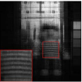
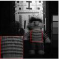
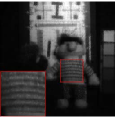
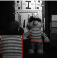
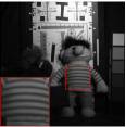
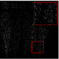
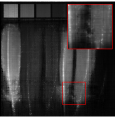
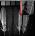
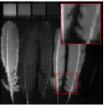
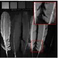
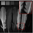
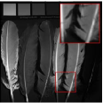
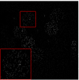
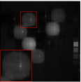
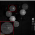
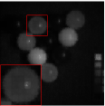
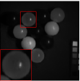
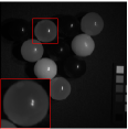
(a) Observed	(b) HaLRTC	(c) tSVD	(d) SiLRTC-TT	(e) TMac-TT	(f) NL-TT	(g) Original

Figure 7: The results of one band of testing MSIs with $SR=0.1$ recovered by different methods. From left to right: (a) the observed image, the results by (b) HaLRTC, (c) tSVD, (d) SiLRTC-TT, (e) TMac-TT, (f) NL-TT, and (g) the original image.

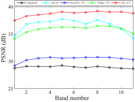
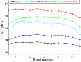
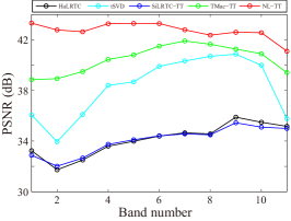
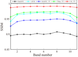
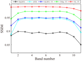
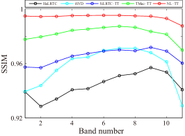
(a) toy	(b) feathers	(c) superballs

Figure 8: The PSNR and SSIM values of all bands of the reconstructed MSIs with $SR=0.2$ recovered by different methods.

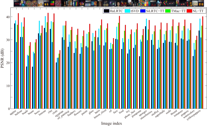
Figure 9: Comparison of the PSNR values by different methods on the dataset CAVE with $SR=0.1$.

Table 3: The average PSNR and SSIM values obtained by HaLRTC, tSVD, SiLRTC-TT, TMac-TT and NL-TT for MSIs with different SRs.

Image	SR	0.05		0.1		0.2
	Method	PSNR	SSIM	PSNR	SSIM	PSNR	SSIM
toy	HaLRTC	20.14	0.6519	23.99	0.7790	28.91	0.8994
	tSVD	25.89	0.7680	30.34	0.8844	36.57	0.9602
	SiLRTC-TT	22.36	0.7138	25.81	0.8392	30.44	0.9433
	TMac-TT	27.28	0.8329	32.37	0.9317	35.74	0.9669
	NL-TT	29.58	0.9243	34.44	0.9730	38.72	0.9899
feathers	HaLRTC	20.66	0.6422	24.26	0.7720	28.81	0.8876
	tSVD	25.15	0.6886	29.29	0.8266	34.82	0.9265
	SiLRTC-TT	22.86	0.7196	26.32	0.8417	31.11	0.9411
	TMac-TT	27.29	0.7611	32.12	0.9190	36.63	0.9631
	NL-TT	29.61	0.9102	34.76	0.9699	39.56	0.9879
superballs	HaLRTC	23.28	0.7661	28.63	0.8621	34.10	0.9426
	tSVD	28.24	0.7636	32.39	0.8663	38.20	0.9564
	SiLRTC-TT	26.27	0.8290	29.79	0.9087	34.03	0.9651
	TMac-TT	29.97	0.8343	33.90	0.9346	40.19	0.9803
	NL-TT	32.93	0.9507	37.25	0.9812	42.67	0.9939

We show one band recovered results in toy, feathers, and superballs by different methods in Fig. 7 and display the PSNR and SSIM values of each band with $SR=0.2$ in Fig. 8. From Fig. 7, the proposed method achieves the best results in preserving the textures and details. From Fig. 8, we see that our method performs higher PSNR and SSIM values than other methods for all bands. Fig. 9 lists the comparison of the PSNR values on all 32 MSIs. Table 3 lists the average performance (over different SRs) of all methods. From these quantitative comparisons, we observe that our method outperforms other competing methods with respect to PSNR and SSIM.

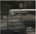
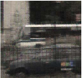
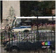
(a) Observed	(b) HaLRTC	(c) tSVD	(d) SiLRTC-TT	(e) TMac-TT	(f) NL-TT	(g) Original

Figure 10: The results of two frames of testing color videos recovered by different methods. The first (third) and second (fourth) rows: the results of color videos bus (mobile), respectively. From left to right: (a) the observed image, the results by (b) HaLRTC, (c) tSVD, (d) SiLRTC-TT, (e) TMac-TT, (f) NL-TT, and (g) the original image.

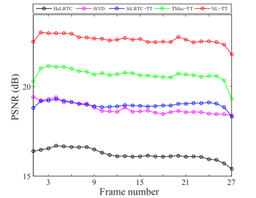
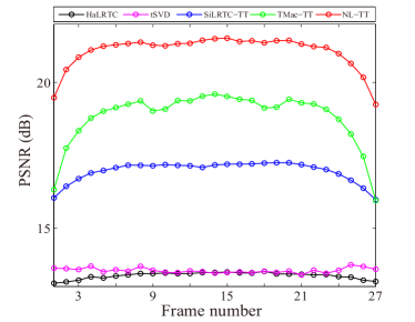
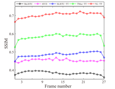
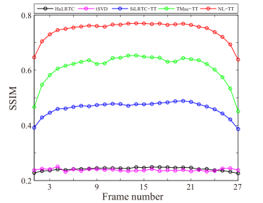
(a) bus	(b) mobile

Figure 11: The PSNR and SSIM values of all frames of color videos recovered by different methods.

6.3 Color videos

In this subsection, we test the proposed method on two color videos $bus$ and $mobile$ with random sampling. The size of testing videos is $243\times 256\times 3\times 27$. The SR is set as 0.1 in this task.

Fig. 10 shows the visual results by using different methods. Obviously, the results by HaLRTC and SiLRTC-TT appear dark and have color distortion, the results by tSVD have undesirable thorns, and the results by our method visually outperforms TMac-TT in keeping smoothness and details of recovered images. The PSNR and SSIM values of each frame of two reconstructed color videos are plotted in Fig. 11. We note that the PSNR and SSIM values of each frame recovered by the proposed method are higher than all compared methods.

7 Discussions

In this section, we test the effects of parameters of the proposed NL-TT method and show the numerical convergence of the ADMM solver. All tests in this section are based on image lena with $SR=0.3$ tube sampling and image house with missing curves as examples.

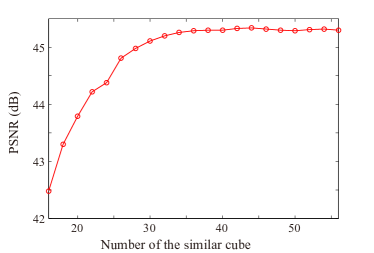
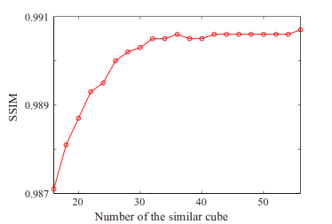
(a) PSNR	(b) SSIM

Figure 12: The PSNR and SSIM curves as the function of the number of the similar cube $h$. (a) change in the PSNR value, (b) change in the SSIM value.

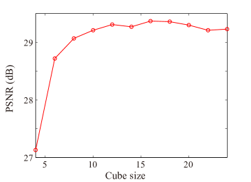
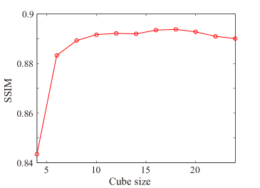
(a) PSNR	(b) SSIM

Figure 13: The PSNR and SSIM curves as the function of the number of the cube size $s$. (a) change in the PSNR value, (b) change in the SSIM value.

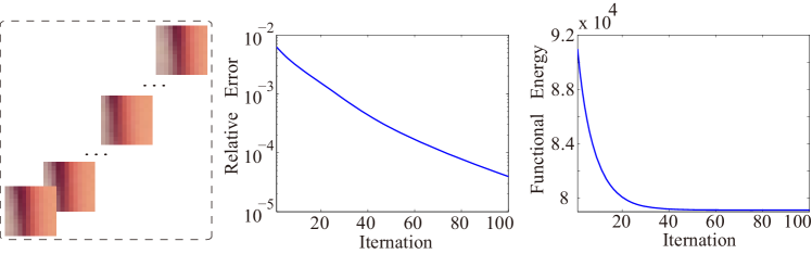
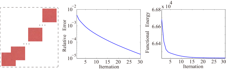
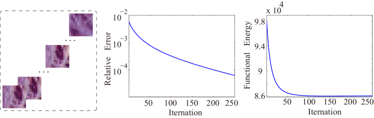
(a) Grouped tensors         (b) Relative error          (c) Function value

Figure 14: The relative error and objective function values curve versus the iteration number for grouped tubes. (a) grouped tensors, (b) change in the relative error value, (c) change in the objective function value.

Effect of the number of the similar cube $h$. In our algorithm, the number of the similar cube $h$ controls the number similar cubes of the grouped tensor. In Fig. 12, we show the experimental results of PSNR and SSIM values as the function of the number $h$ from 16 to 56 with step 2. From Fig. 12, we can observe that when the number of similar cubes is small, the PSNR values increase extremely fast. Then the growing rate of the curve becomes relatively slow. The highest PSNR and SSIM values are achieved around $h=42$. Thus, we empirically choose the number of the similar cube between 30 to 50 with the increment 4.

Effect of the cube size $s$. The cube size $s$ controls the number of patterns in an image cube. Fig. 13 provides the completed results of PSNR and SSIM values as the function of the size $s$ from 4 to 24 with step 2. From Fig. 13, one can observe that a too small $s$ performs poorly. One possible reason is that small-size cubes do not contain enough well-patterned image texture. The highest PSNR and SSIM values are achieved around $s=16$. Therefore, we empirically set the parameter $s\in[10,20]$ with the increment 2.

Numerical convergence. We empirically demonstrate the convergence of the proposed algorithm. Fig. 14 displays the relative error value ($\|\mathcal{X}^{l+1}_{p}-\mathcal{X}^{l}_{p}\|_{F}/\|\mathcal{X}^{l}_{p}\|_{F}$) and the objective function value verse the iteration number for several restored groups. We observe that as the iteration number increases, the relative errors converge to zero and the objective function values tend to flat, which empirically indicates the convergence of the proposed algorithm.

8 Conclusion

In this paper, we propose a new nonlocal TT rank-based tensor completion method by exploring the NSS prior of tensor data. After block-matching, each group of selected $j$-th order cubes are stacked together into a $(j+1)$-th order data. We apply the low-TT-rank constraint on the grouped tensor, which can simultaneously learn the correlation along the spatial, nonlocal, and temporal/spectral modes. Moreover, we establish a perturbation analysis for the TT low-rankness of groups consisting of similar cubes. An efficient ADMM-based algorithm is developed to solve the proposed model. Experiments on color images, MSIs data, and color videos demonstrate the effectiveness of the proposed method. In the future work, we will try to adaptively choose the penalty parameter of each group to enhance the performance and extend the proposed method to other image processing tasks, such as remotely sensed images recovery [9, 15, 21], rain streaks removal [25, 47].

Appendices

Appendix A Proof of Proposition 1

Proof.

We denote the objective function of (5) by $E(\mathcal{X})$. It is clear that $E(\mathcal{X})$ is convex, proper, and continuous. According to the Weierstrass’ theorem [3], it remains only to show the coercivity of $E(\mathcal{X})$, i.e., for every sequence $\{\mathcal{X}^{b}\}$ such that $\|\mathcal{X}^{b}\|_{F}\rightarrow\infty$, we have $\lim_{b\rightarrow\infty}E(\mathcal{X}^{b})=\infty$. We prove it by contradiction. Assume that there exists a subsequence of $\{\mathcal{X}^{b}\}$ (also denoted as $\{\mathcal{X}^{b}\}$) that $\{E(\mathcal{X}^{b})\}$ is bounded, we have that $\sum_{k=1}^{j-1}\alpha_{k}\|\textbf{X}_{[k]}\|_{\ast}$ is bounded. Due to the equivalence of norms, we get that $\{\|\mathcal{X}^{b}\|_{F}\}$ is bounded. Then $\{\mathcal{X}^{b}\}$ is a bounded sequence, which is contradictory with the assumption. So the model (5) has at least one minimizer. ∎

Appendix B Proof of Theorems 1, 2, 3, and 4

Proof of Theorem 1

Proof.

Note that

$$\begin{split}\|\mathcal{E}\|_{F}^{2}=\|\mathcal{X}-\mathcal{Y}\|_{F}^{2}&=\sum_{i_{2}=1}^{s}\sum_{i_{3}=1}^{n_{3}}\sum_{i_{4}=1}^{h}\|\mathcal{X}(:,i_{2},i_{3},i_{4})-\textbf{x}\|_{2}^{2}\\ &\leq sn_{3}h\varepsilon^{2}.\end{split}$$

Therefore, $\|\mathcal{E}\|_{F}\leq\sqrt{sn_{3}h}\varepsilon$. This completes the proof. ∎

Proof of Theorem 2

Proof.

Note that

$$\|\hat{\mathcal{E}}\|_{F}^{2}=\|\mathcal{X}-\hat{\mathcal{Y}}\|_{F}^{2}=\sum_{i_{4}=1}^{h}\|\mathcal{X}(:,:,:,i_{4})-\mathcal{\hat{X}}\|_{F}^{2}\leq h\hat{\varepsilon}^{2}.$$

Therefore, $\|\hat{\mathcal{E}}\|_{F}\leq\sqrt{h}\hat{\varepsilon}$. ∎

Proof of Theorem 3

Proof.

From the definition of $\mathcal{\tilde{E}}$, we get that

$$\begin{split}\|\mathcal{\tilde{E}}\|_{F}^{2}&=\|\mathcal{X}-\mathcal{\tilde{Y}}\|_{F}^{2}\\ &=\sum_{i_{4}=r+1}^{h}\|\mathcal{X}(:,:,:,i_{4})-\mathcal{X}(:,:,:,1)\|_{F}^{2}\\ &\leq(h-r)\tilde{\varepsilon}^{2}.\end{split}$$

Hence $\|\mathcal{\tilde{E}}\|_{F}\leq\sqrt{h-r}\tilde{\varepsilon}$. ∎

Proof of Theorem 4

Proof.

From the definition of $s(\mathcal{X})$, we get that

$$\begin{split}|s(\mathcal{X})-s(\mathcal{Y})|&=\bigg{|}\sum_{k=1}^{3}\alpha_{k}(\|\textbf{X}_{[k]}\|_{\ast}-\|\textbf{Y}_{[k]}\|_{\ast})\bigg{|}\\ &=\bigg{|}\sum_{k=1}^{3}\alpha_{k}\Big{(}\sum_{j_{k}}\big{(}\sigma_{j_{k}}((\textbf{Y+E})_{[k]})-\sigma_{j_{k}}(\textbf{Y}_{[k]})\big{)}\Big{)}\bigg{|}\\ &\leq\sum_{k=1}^{3}\alpha_{k}\Big{(}\sum_{j_{k}}\big{|}\sigma_{j_{k}}((\textbf{Y+E})_{[k]})-\sigma_{j_{k}}(\textbf{Y}_{[k]})\big{|}\Big{)}\\ &\leq\sum_{k=1}^{3}\alpha_{k}\Big{(}\sum_{j_{k}}\big{(}\|\textbf{E}_{[k]}\|_{F}\big{)}\Big{)}\\ &=c\|\mathcal{E}\|_{F}.\\ \end{split}$$

Therefore, $|s(\mathcal{X})-s(\mathcal{Y})|\leq c\|\mathcal{E}\|_{F}$. ∎

References

- [1] J. A. Bengua, H. N. Phiem, H. D. Tuan, and M. N. Do. Efficient tensor completion for color image and video recovery: Low-rank tensor train. IEEE Transactions on Image Processing, 26(5):2466–2479, 2017.
- [2] M. Bertalmio, G. Sapiro, V. Caselles, and C. Ballester. Image inpainting. Siggraph, 4(9):417–424, 2000.
- [3] D. P. Bertsekas, A. Nedic, and A. E. Ozdaglar. Convex analysis and optimization. Athena Scientific, 2003.
- [4] J-F. Cai, E. J. Cands, and Z. Shen. A singular value thresholding algorithm for matrix completion. SIAM Journal on Optimization, 20(4):1956–1982, 2008.
- [5] R. H. Chan, M. Tao, and X. Yuan. Constrained total variation deblurring models and fast algorithms based on alternating direction method of multipliers. SIAM Journal on Imaging Sciences, 6(1):680–697, 2013.
- [6] S. H. Chan, R. Khoshabeh, K. B. Gibson, P. E. Gill, and T. Q. Nguyen. An augmented Lagrangian method for total variation video restoration. IEEE Transactions on Image Processing, 20(11):3097–3111, 2011.
- [7] Y. Chang, L-X. Yan, and S. Zhong. Hyper-laplacian regularized unidirectional low-rank tensor recovery for multispectral image denoising. In IEEE Conference on Computer Vision and Pattern Recognition, pages 5901–5909, 2017.
- [8] Y. Chen, C. Hsu, and H. M. Liao. Simultaneous tensor decomposition and completion using factor priors. IEEE Transactions on Pattern Analysis and Machine Intelligence, 36(3):577–591, 2014.
- [9] Y. Chen, T-Z. Huang, and X-L. Zhao. Destriping of multispectral remote sensing image using low-rank tensor decomposition. IEEE Journal of Selected Topics in Applied Earth Observations and Remote Sensing, 11(12):4950–4967, 2018.
- [10] K. Dabov, A. Foi, V. Katkovnik, and K. Egiazarian. Image denoising by sparse 3-D transform-domain collaborative filtering. IEEE Transactions on Image Processing, 16(8):2080–2095, 2007.
- [11] M. Ding, T-Z. Huang, T-Y. Ji, X-L. Zhao, and J-H. Yang. Low-rank tensor completion using matrix factorization based on tensor train rank and total variation. Journal of Scientific Computing, 81:941–964, 2019.
- [12] Y. Du, G. Han, Y. Quan, Z. Yu, H. Wong, C. L. P. Chen, and J. Zhang. Exploiting global low-rank structure and local sparsity nature for tensor completion. IEEE Transactions on Cybernetics, 49(11):3898–3910, 2019.
- [13] J. Eckstein and D. P. Bertsekas. On the Douglas-Rachford splitting method and the proximal point algorithm for maximal monotone operators. Mathematical Programming, 55(1):293–318, 1992.
- [14] G. Ely, S. Aeron, N. Hao, and M. E. Kilmer. 5D seismic data completion and denoising using a novel class of tensor decompositions. GEOPHYSICS, 80(4):V83–V95, 2015.
- [15] X. Fu, K-J. Huang, B. Yang, W. K. Ma, and N. D. Sidiropoulos. Robust volume minimization-based matrix factorization for remote sensing and document clustering. IEEE Transactions on Signal Processing, 64(23):6254–6268, 2016.
- [16] S. Gandy, B. Recht, and I. Yamada. Tensor completion and low-n-rank tensor recovery via convex optimization. Inverse Problems, 27(2):025010, 2011.
- [17] T. Goldstein, B. O’Donoghue, S. Setzer, and R. Baraniuk. Fast alternating direction optimization methods. SIAM Journal on Imaging Sciences, 7(3):1588–1623, 2014.
- [18] L. Grasedyck, M. Kluge, and S. Krämer. Alternating least squares tensor completion in the TT-format. arXiv preprint arXiv:1509.00311.
- [19] S-H. Gu, L. Zhang, W-M. Zuo, and X-C. Feng. Weighted nuclear norm minimization with application to image denoising. In IEEE Conference on Computer Vision and Pattern Recognition, pages 2862–2869, 2014.
- [20] B-S. He and X. Yuan. On the O(1/n) convergence rate of the Douglas-Rachford alternating direction method. SIAM Journal on Numerical Analysis, 50(2):700–709, 2012.
- [21] W. He, H-Y. Zhang, L-P. Zhang, and H-F. Shen. Total-variation-regularized low-rank matrix factorization for hyperspectral image restoration. IEEE Transactions on Geoscience and Remote Sensing, 54(1):176–188, 2016.
- [22] C. J. Hillar and L. H. Lim. Most tensor problems are NP-hard. Journal of the ACM, 60(6):45:1–45, 2013.
- [23] Y-M. Huang, H-Y. Yan, Y-W. Wen, and X. Yang. Rank minimization with applications to image noise removal. Information Sciences, 429:147–163, 2018.
- [24] T-Y. Ji, T-Z. Huang, X-L. Zhao, T-H. Ma, and G. Liu. Tensor completion using total variation and low-rank matrix factorization. Information Sciences, 326:243–257, 2016.
- [25] T-X. Jiang, T-Z. Huang, X-L. Zhao, L-J. Deng, and Y. Wang. FastDeRain: A novel video rain streak removal method using directional gradient priors. IEEE Transactions on Image Processing, 28(4):2089–2102, 2019.
- [26] M. E. Kilmer, K. Braman, N. Hao, and R. C. Hoover. Third-order tensors as operators on matrices: A theoretical and computational framework with applications in imaging. SIAM Journal on Matrix Analysis and Applications, 34(1):148–172, 2013.
- [27] T. G. Kolda and B. W. Bader. Tensor decompositions and applications. SIAM Review, 51(3):455–500, 2009.
- [28] T. G. Kolda, B. W. Bader, and J. P. Kenny. Higher-order web link analysis using multilinear algebra. In IEEE International Conference on Data Mining, pages 242–249, 2005.
- [29] N. Komodakis. Image completion using global optimization. In IEEE Conference on Computer Vision and Pattern Recognition, volume 1, pages 442–452, 2006.
- [30] J. I. Latorre. Image compression and entanglement. Computer Science, 2005.
- [31] F. Li, M. K. Ng, and R. J. Plemmons. Coupled segmentation and denoising/deblurring models for hyperspectral material identification. Numerical Linear Algebra with Applications, 19(1):153–173, 2012.
- [32] J. Liu, P. Musialski, P. Wonka, and J. Ye. Tensor completion for estimating missing values in visual data. IEEE Transactions on Pattern Analysis and Machine Intelligence, 35(1):208–220, 2013.
- [33] Y.-P. Liu, Z. Long, H.-Y. Huang, and C. Zhu. Low CP rank and Tucker rank tensor completion for estimating missing components in image data. IEEE Transactions on Circuits and Systems for Video Technology, pages 1–11, 2019, http://dx.doi.org/10.1109/TCSVT.2019.2901311.
- [34] Y.-P. Liu, Z. Long, and C. Zhu. Image completion using low tensor tree rank and total variation minimization. IEEE Transactions on Multimedia, 21(2):338–350, 2019.
- [35] Y-Y. Liu, F-H. Shang, L-C. Jiao, J. Cheng, and H. Cheng. Trace norm regularized CANDECOMP/PARAFAC decomposition with missing data. IEEE Transactions on Cybernetics, 45(11):2437–2448, 2015.
- [36] C-Y. Lu, J-S. Feng, Y-D. Chen, W. Liu, Z-C. Lin, and S-C. Yan. Tensor robust principal component analysis: Exact recovery of corrupted low-rank tensors via convex optimization. In IEEE Conference on Computer Vision and Pattern Recognition, pages 5249–5257, 2016.
- [37] C-Y. Lu, J-S. Feng, Z-C. Lin, and S-C. Yan. Exact low tubal rank tensor recovery from gaussian measurements. In International Joint Conference on Artificial Intelligence, 2018.
- [38] T-H. Ma, T-Z. Huang, and X-L. Zhao. Group-based image decomposition using 3-D cartoon and texture priors. Information Sciences, 328:510–527, 2016.
- [39] J-J. Mei, Y-Q. Dong, T-Z. Huang, and W-T. Yin. Cauchy noise removal by nonconvex admm with convergence guarantees. Journal of Scientific Computing, 74:743–766, 2018.
- [40] I. V. Oseledets. Tensor-train decomposition. SIAM Journal on Scientific Computing, 33(5):2295–2317, 2011.
- [41] E. E. Papalexakis, C. Faloutsos, and N. D. Sidiropoulos. Tensors for data mining and data fusion: Models, applications, and scalable algorithms. ACM Transactions on Intelligent Systems and Technology, 8(2):16:1–16:44, 2017.
- [42] N. D. Sidiropoulos, L. De Lathauwer, X. Fu, K. Huang, E. E. Papalexakis, and C. Faloutsos. Tensor decomposition for signal processing and machine learning. IEEE Transactions on Signal Processing, 65(13):3551–3582, 2017.
- [43] G. W. Stewart. Matrix Algorithms, Vol I: Basic Decomposition. SIAM, 2001.
- [44] W. Wang, V. Aggarwal, and S. Aeron. Tensor completion by alternating minimization under the tensor train (TT) model. arXiv preprint arXiv:1609.05587.
- [45] Y. Wang, D-Y. Meng, and M. Yuan. Sparse recovery: from vectors to tensors. National Science Review, 5(5):756–767, 2018.
- [46] Y. Wang, J-J. Peng, Q. Zhao, Y. Leung, X-L. Zhao, and D-Y. Meng. Hyperspectral image restoration via total variation regularized low-rank tensor decomposition. IEEE Journal of Selected Topics in Applied Earth Observations and Remote Sensing, 11(4):1227–1243, 2018.
- [47] Y-T. Wang, X-L. Zhao, T-X. Jiang, L-J. Deng, T-H. Ma, Y-T. Zhang, and T-Z. Huang. A total variation and group sparsity based tensor optimization model for video rain streak removal. Signal Processing: Image Communication, 73:96–108, 2019.
- [48] Z-M. Xing, M-Y. Zhou, A. Castrodad, G. Sapiro, and L. Carin. Dictionary learning for noisy and incomplete hyperspectral images. SIAM Journal on Imaging Sciences, 5(1):33–56, 2012.
- [49] Y-Y. Xu, R-R. Hao, W-T. Yin, and Z-X. Su. Parallel matrix factorization for low-rank tensor completion. Inverse Problems and Imaging, 9(2):601–624, 2017.
- [50] T. Yokota, Q-B. Zhao, C. Li, and A. Cichocki. Smooth PARAFAC decomposition for tensor completion. IEEE Transactions on Signal Processing, 64(20):5423–5436, 2016.
- [51] K-B. Zhang, X-B. Gao, D-C. Tao, and X-L. Li. Single image super-resolution with non-local means and steering kernel regression. IEEE Transactions on Image Processing, 21(11):4544–4556, 2012.
- [52] X-J. Zhang. A nonconvex relaxation approach to low-rank tensor completion. IEEE Transactions on Neural Networks and Learning Systems, 30(6):1659–1671, 2019.
- [53] Z. Zhang, G. Ely, and S Aeron. Exact tensor completion using t-SVD. IEEE Transactions on Signal Processing, 65(6):1511–1526, 2017.
- [54] Q-B. Zhao, L-Q. Zhang, and A. Cichocki. Bayesian cp factorization of incomplete tensors with automatic rank determination. IEEE Transactions on Pattern Analysis and Machine Intelligence, 37(9):1751–1763, 2015.
- [55] X-L. Zhao, F. Wang, T-Z. Huang, M. K. Ng, and R. J. Plemmons. Deblurring and sparse unmixing for hyperspectral images. IEEE Transactions on Geoscience and Remote Sensing, 51(7):4045–4058, 2013.
- [56] Y-B. Zheng, T-Z. Huang, T-Y. Ji, X-L. Zhao, T-X. Jiang, and T-H. Ma. Low-rank tensor completion via smooth matrix factorization. Applied Mathematical Modelling, 70:677–695, 2019.