Rotating five-dimensional electrically charged Bardeen regular black holes

Abstract

We derive a rotating counterpart of the five-dimensional electrically charged Bardeen regular black holes spacetime by employing the Giampieri algorithm on static one. The associated nonlinear electrodynamics source is computed in order to justify the rotating solution. We thoroughly discuss the energy conditions and the other properties of the rotating spacetime. The black hole thermodynamics of the rotating spacetime is also presented. In particular, the thermodynamic quantities such as the Hawking temperature and the heat capacity are calculated and plotted to see the thermal behavior. The Hawking temperature profile of the black hole implies that the regular black holes are thermally colder than its singular counterpart. On the other hand, we find that the heat capacity has two branches: the negative branch corresponds to the unstable phase and the positive branch corresponds to that of the stable phase for a suitable choice of the physical parameters characterizing the black holes.

I Introduction

The existence of the equivalence principle and the connection between gravity and thermodynamics are two of the most fascinating features of gravity. Between these two, the principle of equivalence finds its natural expression when gravity is described as a manifestation of curved spacetime Padmanabhan:2002ma . Black holes are the automatic consequence of the Einstein’s field equations. The first exact mathematical solution of black holes was discovered by Karl Schwarzschild widely known as the Schwarzschild solution Schwarzschild:1916 , which describes a static spherically symmetric spacetime. However, the charged version of the Schwarzschild solution is known as the Reissner-Nordström solution Reissner:1916 . After the proposal of these spacetimes various solutions of black holes have been discovered. Black holes have not been only studied in four dimensions but also there are many higher dimensional solutions available in the literature. The observational detection of gravitational waves by advanced LIGO/Virgo is strong confirmation of the existence of black holes Abbott:2016blz ; Abbott:2016nmj ; TheLIGOScientific:2016pea . Recent observations by the Event Horizon Telescope revealed the first image of suppermassive black hole, namely M87 Akiyama:2019fyp ; Akiyama:2019eap .

Finding exact solutions of the Einstein’s field equations is a nontrivial task and a very important branch of general relativity. In general relativity, it is always challenging to discover an axisymmetric or rotating solution in four dimensions as well as in higher dimensions. Roy Kerr obtained the well-known axisymmetric solution Kerr:1963ud ; it was discovered by imposing the stationary and axial symmetric conditions on the Einstein’s field equations Kerr:1963ud . Physically, these rotating solutions have paramount importance because it is believed that most of the astrophysical black holes are rotating or Kerr-like. In 1965, Newman and Janis discovered an alternative approach to obtain the same Kerr metric by imposing a set of complex coordinate transformations on the Schwarzschild metric Newman:1965tw . Through these transformations angular momenta are added to the static seed metric; this is widely known as the Newman Janis Algorithm (NJA). Furthermore, an alternative derivation of the Kerr-Newman metric is derived from the Reissner-Nordström seed metric by using the same algorithm Newman:1965my . There exists a wide range of rotating solutions, discovered through this algorithm Demianski:1966 ; Demianski:1972uza ; Herrera:1982 ; Erbin:2016lzq ; Kim:1998iw ; Yazadjiev:1999ce . The NJA approach has also been used to describe the Kerr interiors from static metrices Drake:1997hh . Apart from NJA, several other methods have been developed to generate the rotating solutions from the static ones Clement:1997tx ; Drake:1998gf ; Glass:2004rr ; Gibbons:2004uw ; Kim:2012pb ; Murenbeeld:1970aq . Giampieri Giampieri:1990 proposed another alternative algorithm to generate the rotating metric in a much more simple way than the NJA. This algorithm requires neither calculation of the null tetrad basis nor is the metric to be inverted. It is noticeable that the results discovered through both of these techniques are exactly same. Recently, this algorithm was used by the authors in Erbin:2014lwa ; Mirzaiyan:2017adt to obtain successfully the five-dimensional Myers-Perry solution Myers:1986un from the static Schwarzschild-Tangherlini seed metric. Since the null tetrad calculation is very tedious while working in higher dimensions Myers:1986un ; Dianyan:1988 , this algorithm may be very helpful in extending to higher dimensions.

Our main motive of this paper is to apply the Giampieri algorithm on the five-dimensional electrically charged static Bardeen regular spacetime in order to obtain a rotating spacetime having two distinct spin parameters. Moreover, our main motivation in th work is to discuss the various properties of the rotating spacetime, e.g., horizons, static limit surfaces, and ergosphere. As we already know that the Bardeen spacetime represents a singularity free black hole spacetime. It is a general belief that black holes contain spacetime singularities and the cosmic censorship conjecture claims that these spacetime singularities are covered by the event horizon. Their presence breaks down the standard physical laws and hence it provides limitations to general relativity. Quantum gravity is the expected theory that might be capable to resolve the singularity problem. This theory discusses very tiny scale physics (at the Planck scale), but we are still far away from achieving this. It is required that we consider some alternative approaches that are somehow able to remove or to avoid these spacetime singularities. One of the possible approach to obtain such nonsingular nature of the spacetime is the prediction of the regular black hole solutions where a central singularity is replaced by a de-Sitter belt. These solutions contain an event horizon but not any spacetime singularity within them. The spacetime singularities are avoided either by introducing some exotic field in the form of nonlinear electrodynamics or by some modification to gravity. Bardeen applied the idea of Sakharov Sakharov:1966 to replace the spacetime singularity by a de Sitter core, and described the first black hole solution without any spacetime singularity Bardeen:1968 . The physical source associated with Bardeen black hole was described in AyonBeato:2000zs . The rotating Bardeen solution is proposed in Bambi:2013ufa , in which the authors applied NJA on the Bardeen solution Bardeen:1968 . After the discovery of the Bardeen solution several regular static and rotating black hole solutions has been published in literature, which successively overcome spacetime singularities AyonBeato:1998ub ; AyonBeato:1999ec ; Dymnikova:2004zc ; Bronnikov:2000vy ; Shankaranarayanan:2003qm ; Hayward:2005gi ; Culetu:2014lca ; Balart:2014cga ; Toshmatov:2014nya ; Ghosh:2014hea ; Neves:2014aba ; Azreg-Ainou:2014nra ; Azreg-Ainou:2014pra ; Ghosh:2014pba . Recently, the $d$-dimensional Bardeen-de Sitter black holes are presented Ali:2018boy and regular black holes in Einstein-Gauss-Bonnet gravity are also obtained Ghosh:2018bxg ; Kumar:2018vsm .

The paper is organized as follows. We discuss the five-dimensional electrically charged Bardeen regular black hole spacetime in Sec. II. In Sec. III, we employ the Giampieri algorithm on the static metric and obtain a rotating five-dimensional electrically charged Bardeen regular spacetime. The energy conditions of the rotating spacetime are analysed in Sec. IV and the nature of the spacetime in Sec. V. Black hole thermodynamics is the subject of Sec. VI. We conclude by discussing our main results in Sec. VII.

II Electrically charged Bardeen regular black holes

The dynamics of the spacetime is governed by the action, therefore, the Einstein-Hilbert action coupled to the nonlinear electrodynamics in five dimensions can be written as follows

$$I=\frac{1}{16\pi}\int{d^{5}{x}\sqrt{-g}\left[R-4\mathcal{L}\left(\mathcal{F}\right)\right]},$$ (1)

where $R$ is the Ricci scalar and $g$ is related to the determinant of spacetime metric. The Lagrangian $\mathcal{L}(\mathcal{F})$ is a nonlinear function of the electromagnetic field strength $\mathcal{F}=F_{\mu\nu}F^{\mu\nu}/4$ where $F_{\mu\nu}=\partial_{\mu}A_{\nu}-\partial_{\nu}A_{\mu}$, and $A_{\mu}$ is the gauge potential. The Einstein’s field equations can be derived by the variation of action (1) with respect to $g_{\mu\nu}$, which yields

$$R_{\mu\nu}-\frac{1}{2}g_{\mu\nu}R = T_{\mu\nu}.$$ (2)

However, the energy-momentum tensor $T_{\mu\nu}$ is given by

$$T_{\mu\nu}=2\left(\mathcal{L}_{\mathcal{F}}F_{\mu\alpha}F_{\nu}^{\alpha}-g_{\mu\nu}\mathcal{L}\right),$$ (3)

where $\mathcal{L}_{\mathcal{F}}=\partial\mathcal{L}/\partial\mathcal{F}$. On the other hand, the Maxwell equations can be obtained by varying the action with respect to gauge potential $A_{\mu}$, which read simply

$$\nabla_{\mu}\left(\mathcal{L}_{\mathcal{F}}F^{\mu\nu}\right) = 0.$$ (4)

The static spacetime metric of the five-dimensional electrically charged Bardeen regular black hole Ali:2018boy is given by

$$ds^{2} = -f(r)dt^{2}+f(r)^{-1}dr^{2}+r^{2}\left(d\theta^{2}+\sin^{2}\theta d\phi^{2}+\cos^{2}\theta d\psi^{2}\right),$$ (5)

with

$$f(r)=1-\frac{\mu r^{2}}{(r^{3}+q_{e}^{3})^{4/3}},$$ (6)

where the free parameters $q_{e}$ and $\mu$ are related to the electric charge and black hole mass, respectively. The metric function $f(r)$ for large and small $r$, respectively, reads

$$f(r)\sim 1-\frac{\mu}{r^{2}},\quad f(r)\sim 1-\frac{\mu}{q_{e}^{4}}r^{2}.$$ (7)

In order to obtain the electromagnetic tensor, we solve the Maxwell equations (4). The four dimensional solution of electrically charged Bardeen black hole has been discussed by Rodrigues et al. Rodrigues:2018bdc . The non-vanishing components of the electromagnetic tensor are $F_{01}$ and $F_{10}$, which read simply

$$F_{01}=\frac{q_{e}}{\mathcal{L}_{\mathcal{F}}(r)r^{3}}=-F_{10}.$$ (8)

Therefore, the electromagnetic field strength takes the following form,

$$\mathcal{F}=-\frac{q_{e}^{2}}{2\mathcal{L}_{\mathcal{F}}^{2}(r)r^{6}}.$$ (9)

We further solve the Einstein’s field equations in order to obtain the expressions of $\mathcal{L}(r)$ and $\mathcal{L}_{\mathcal{F}}(r)$, as

$$\mathcal{L}(r) = \frac{\mu q_{e}^{3}\left(3q_{e}^{3}-4r^{3}\right)}{\left(r^{3}+q_{e}^{3}\right)^{10/3}},$$

$$\mathcal{L}_{\mathcal{F}}(r) = \frac{\left(r^{3}+q_{e}^{3}\right)^{10/3}}{7\mu q_{e}r^{9}}.$$ (10)

These equations when substitute back into the Einstein field equations, they satisfy them. The corresponding gauge potential can be expressed as following

$$A^{\mu}=-\frac{\mu r^{7}}{q_{e}\left(r^{3}+q_{e}^{3}\right)^{7/3}}\delta^{\mu}_{t}.$$ (11)

A substitution of $\mathcal{L}_{\mathcal{F}}(r)$ from (II) into (9) yields

$$\mathcal{F}=-\frac{49\mu^{2}q_{e}^{4}r^{12}}{2\left(r^{3}+q_{e}^{3}\right)^{20/3}}.$$ (12)

In order to verify that the spacetime (5) does not contain any spacetime singularity, we need to obtain the expressions of the curvature invariants, and check whether they diverge or give finite value in the limit $r\rightarrow 0$. We can compute these limits as follows

$$\lim_{r\rightarrow 0}R=\frac{20\mu}{q_{e}^{4}},\quad\lim_{r\rightarrow 0}\mathcal{R}=\frac{80\mu^{2}}{q_{e}^{8}},\quad\lim_{r\rightarrow 0}K=\frac{40\mu^{2}}{q_{e}^{8}}.$$ (13)

It is clear that the black hole interior does not terminate in a singularity but crosses the Cauchy horizon and develops in a region that becomes more and more de-Sitter like and eventually ending with a regular origin at $r=0$. Now let us step forward to achieve our goal to describe the rotating counterpart of this solution.

III Rotating five-dimensional electrically charged Bardeen regular black holes

In this section, we formulate the rotating counterpart of the five-dimensional electrically charged Bardeen regular spacetime by employing the Giampieri algorithm on the static metric. The Giampieri algorithm is much simpler algorithm to generate the rotating solution in comparison to the Newman-Janis algorithm (NJA). A very simple reason is of course this algorithm avoids the tedious null tetrads calculation. The important feature that we encounter in NJA is the fact that a given set of transformations in $(r,\phi)$-plane generates rotation in the later. The generation of two different angular momenta in two different planes would then require successive applications of the NJA on different hypersurfaces. In five dimensions, the two different planes that can be made rotating are the $(r,\phi)$ and $(r,\psi)$ planes. In order to do that we need to dissociate the radii of the two planes in order to apply the NJA on each plane and thereby generating two different angular momenta in respective planes. The important thing about this prescription is that we employ it to generate five-dimensional doubly rotating spacetime. We must dissociate the parts of the metric that correspond to the rotating and nonrotating two-planes. Therefore, one has to take care of the $r^{2}$-term from transforming under complex transformation in the part of the metric defining the plane which will stay static.

Let us move forward step by step to construct the rotating five-dimensional electrically charged Bardeen regular black hole spacetime. The first step of the Giampieri algorithm is similar to that of NJA where we need to write down the metric (5) in the Edington-Finklestein retarded null coordinates. In addition, we introduce a function $R(r)=Re(r)$ such that the metric in null coordinates is written Erbin:2014lwa as follows

$$ds^{2}=-du(du+2dr)+(1-f(r))du^{2}+r^{2}\left(d\theta^{2}+\sin^{2}\theta d\phi^{2}\right)+R^{2}\cos^{2}\theta d\psi^{2}.$$ (14)

The coordinates $u$ and $r$ must be complex and the metric (14) transformed in $(r,\phi)$-plane by the following coordinate transformations

$$u = u^{\prime}+ia\cos\chi_{1},\quad r=r^{\prime}-ia\cos\chi_{1},$$ (15)

where $\chi_{1}$ is a new angle. The differential transformations of (15) are given by

$$du = du^{\prime}-a\sin^{2}\theta d\phi,\quad dr=dr^{\prime}+a\sin^{2}\theta d\phi,$$ (16)

where we use the ansatz $id\chi_{1}=\sin\chi_{1}d\phi$ and $\chi_{1}=\theta$. On applying the complex transformations (15) and (16) on metric (14) as well as by replacing the metric function $f(r)$ with $\tilde{f}^{\{1\}}=\tilde{f}^{\{1\}}(r,\theta)$, and after omitting the primes, we obtain

$$ds^{2} = -du^{2}-2dudr+\left(1-\tilde{f}^{\{1\}}\right)\left(du-a\sin^{2}\theta d\phi\right)^{2}+2a\sin^{2}\theta drd\phi$$ (17)

$$+(r^{2}+a^{2}\cos^{2}\theta)d\theta^{2}+(r^{2}+a^{2})\sin^{2}\theta d\phi^{2}+r^{2}\cos^{2}\theta d\psi^{2},$$

where the new form of metric function $\tilde{f}^{\{1\}}$ is given as follows

$$\tilde{f}^{\{1\}}=1-\frac{\tilde{m}(r,\theta)}{|r|^{2}}=1-\frac{\tilde{m}(r,\theta)}{r^{2}+a^{2}\cos^{2}\theta}.$$ (18)

Since the function $f(r)$ has to be transformed twice under the complex transformation, we need to keep track of the order of the transformations. Now we employ the following transformations in order to transform the metric (14) into the $(r,\psi)$-plane

$$u = u^{\prime}+ib\cos\chi_{2},\quad r=r^{\prime}-ib\cos\chi_{2},$$

$$id\chi_{2} = -\cos\chi_{2}d\psi,\quad\mbox{with}\quad\chi_{2}=\theta,$$

$$du = du^{\prime}-b\cos^{2}\theta d\psi,\quad dr=dr^{\prime}+b\cos^{2}\theta d\psi.$$ (19)

When these transformations are applied directly to the metric (14), yields

$$ds^{2} = -du^{2}-2dudr+\left(1-\tilde{f}^{\{2\}}\right)\left(du-a\sin^{2}\theta d\psi\right)^{2}+2a\sin^{2}\theta dRd\phi+\rho^{2}d\theta^{2}$$ (20)

$$+\left(R^{2}+a^{2}\right)\sin^{2}\theta d\phi^{2}+r^{2}\cos^{2}\theta d\psi^{2}.$$

Keep in mind that once again we need to choose the function $R(r)=Re(r)$ to protect the geometry of the first plane under these complex transformations. On imposing $R=r^{\prime}$ and omitting the prime, we arrive on the new form of the metric containing two distinct spin parameters

$$ds^{2} = -du^{2}-2dudr+\left(1-\tilde{f}^{\{1,2\}}\right)\left(du-a\sin^{2}\theta d\phi-b\cos^{2}\theta d\psi\right)^{2}+2a\sin^{2}\theta drd\phi$$ (21)

$$+2b\cos^{2}\theta drd\psi+\rho^{2}d\theta^{2}+\left(r^{2}+a^{2}\right)\sin^{2}\theta d\phi^{2}+\left(r^{2}+b^{2}\right)\cos^{2}\theta d\psi^{2}$$

with

$$\rho^{2}=r^{2}+a^{2}\cos^{2}\theta+b^{2}\sin^{2}\theta.$$ (22)

The metric function $\tilde{f}^{\{1,2\}}$ is complexified as follows

$$\tilde{f}^{\{1,2\}}=1-\frac{\tilde{m}(|r|,\theta)}{|r|^{2}+a^{2}\cos^{2}\theta}=1-\frac{\tilde{m}_{\tilde{\alpha},\tilde{\beta}}(r^{\prime},\theta)}{r{{}^{\prime}}^{2}+a^{2}\cos^{2}\theta+b^{2}\sin^{2}\theta}=1-\frac{\tilde{m}_{\tilde{\alpha},\tilde{\beta}}(r,\theta)}{\rho^{2}}.$$ (23)

On the other hand, the mass function $\tilde{m}_{\tilde{\alpha},\tilde{\beta}}(r,\theta)$ is complexified

$$m(r)=\tilde{m}(|r|,\theta)=\tilde{m}_{\tilde{\alpha},\tilde{\beta}}(r^{\prime},\theta)=\tilde{m}_{\tilde{\alpha},\tilde{\beta}}(r,\theta)=\mu\Bigg{[}\frac{r^{3+\tilde{\alpha}}(\rho^{2})^{-\tilde{\alpha}}}{r^{3+\tilde{\alpha}}(\rho^{2})^{-\tilde{\alpha}/2}+q_{e}^{3}r^{\tilde{\beta}}(\rho^{2})^{-\tilde{\beta}/2}}\Bigg{]}^{4/3},$$ (24)

where $\tilde{\alpha}$ and $\tilde{\beta}$ are two real numbers appearing during the complexification. For the matter of simplicity, we set $\tilde{\alpha}=\tilde{\beta}=0$, in this case the mass function looks like

$$m(r)=\mu\left(\frac{r^{3}}{r^{3}+q_{e}^{3}}\right)^{4/3}.$$ (25)

Now let us transform the metric (21) into Boyer-Lindquist coordinates with the help of the following coordinate transformations

$$du=dt-g_{1}(r)dr,\quad d\phi=d\phi^{\prime}-g_{2}(r)dr,\quad d\psi=d\psi^{\prime}-g_{3}(r)dr.$$ (26)

On imposing the conditions $g_{tr}=g_{r\phi\prime}=g_{r\psi\prime}=0$, in order to solve (26) for $g_{1}(r)$, $g_{2}(r)$, and $g_{3}(r)$, we obtain

$$g_{1}(r)=\frac{\Pi}{\Delta},\quad g_{2}(r)=\frac{\Pi}{\Delta}\frac{a}{r^{2}+a^{2}},\quad g_{3}(r)=\frac{\Pi}{\Delta}\frac{b}{r^{2}+b^{2}},$$ (27)

where $\Pi$ and $\Delta$ are given by

$$\Pi=\left(r^{2}+a^{2}\right)\left(r^{2}+b^{2}\right),\quad\Delta=\left(r^{2}+a^{2}\right)\left(r^{2}+b^{2}\right)-m(r)r^{2}.$$ (28)

We further apply the Boyer-Lindquist coordinate transformations (26) on the metric (21), as a consequence we get the final form of the five-dimensional rotating spacetime

$$ds^{2} = -dt^{2}+\left(1-\tilde{f}^{\{1,2\}}\right)\left(dt-a\sin^{2}\theta d\phi-b\cos^{2}\theta d\psi\right)^{2}+\frac{r^{2}\rho^{2}}{\Delta}dr^{2}$$ (29)

$$+\rho^{2}d\theta^{2}+\left(r^{2}+a^{2}\right)\sin^{2}\theta d\phi^{2}+\left(r^{2}+b^{2}\right)\cos^{2}\theta d\psi^{2}.$$

Here the angles $\phi$ and $\psi$ lies in the interval $[0,2\pi]$ while the angle $\theta$ takes values from the interval $[0,\pi/2]$. When we substitute function $\tilde{f}^{\{1,2\}}$ into (29), eventually it reads simply

$$ds^{2} = -dt^{2}+\frac{m(r)}{\rho^{2}}\left(dt-\omega\right)^{2}+\frac{r^{2}\rho^{2}}{\Delta}dr^{2}+\rho^{2}d\theta^{2}$$ (30)

$$+\left(r^{2}+a^{2}\right)\sin^{2}\theta d\phi^{2}+\left(r^{2}+b^{2}\right)\cos^{2}\theta d\psi^{2},$$

where $\omega$ is defined as follows

$$\omega=a\sin^{2}\theta d\phi+b\cos^{2}\theta d\psi.$$ (31)

We must emphasize that as like the Meyers-Perry black hole, the rotating five-dimensional electrically charged Bardeen spacetime has two rotation parameters ($a$ and $b$). Note that the rotation is along the ($\phi,\psi$) axes, where $0\leq\phi\leq 2\pi$ and $0\leq\psi\leq\pi/2$. We recover the Meyers-Perry spacetime, in the limit $q_{e}\to 0$. Hence, we reach at the conclusion that the presence of charge $q_{e}$ provides deviation from the Meyers-Perry spacetime.

Now we are going to check the validity of the rotating five-dimensional spacetime by computing the source nonlinear electrodynamics expressions. The gauge potential (11) for the rotating spacetime gets modify Aliev:2004ec as follows

$$A^{\mu}=-\frac{\mu r^{7}}{q_{e}\left(r^{3}+q_{e}^{3}\right)^{7/3}}\left(\delta^{\mu}_{t}-a\sin^{2}\theta\delta^{\mu}_{\phi}-b\cos^{2}\theta\delta^{\mu}_{\psi}\right).$$ (32)

On using this gauge potential, it is easy to compute the field strength $(\mathcal{F})$ in case of the rotating spacetime which turns out to be in following form

$$\mathcal{F}=\frac{\mu^{2}r^{12}\left[-Gmr^{2}+\rho^{2}\{J(a^{2}-b^{2})\cos^{2}\theta+N(r^{2}+a^{2})\}\right]}{2\Delta\rho^{4}q_{e}^{2}\left(r^{3}+q_{e}^{3}\right)^{20/3}},$$ (33)

where $G=49q_{e}^{6}(r^{4}+b^{4})-4b^{2}r^{5}(r^{3}+2q_{e}^{3})+2(a^{2}-b^{2})\cos^{2}\theta(49b^{2}q_{e}^{6}+47q_{e}^{6}r^{2}-4q_{e}^{3}r^{5}-2r^{8})+49q_{e}^{6}(a^{2}-b^{2})\cos^{4}\theta+94b^{2}q_{e}^{6}r^{2}$, $J=49q_{e}^{6}r^{2}(a^{2}+b^{2})-4r^{7}(r^{3}+2q_{e}^{3})+49a^{2}b^{2}q_{e}^{6}+45q_{e}^{6}r^{4}$, and $N=49q_{e}^{6}(r^{2}+b^{2})^{2}-4b^{2}r^{2}(r^{3}+q_{e}^{3})^{2}$. We immediately recover $\mathcal{F}$ exactly as (12) when substitute $a=b=0$ in (33). Our next task is to determine the source for the rotating spacetime. We solve Einstein field equations of the rotating five-dimensional spacetime in order to calculate $\mathcal{L}$ and $\mathcal{L}_{\mathcal{F}}$. It turns out that the Lagrangian density is given by

$$\mathcal{L}(r)=\frac{49\Delta m^{\prime\prime}\rho^{4}q_{e}^{6}(\Delta+mr^{2})+2rm^{\prime}(a^{2}-b^{2})\cos^{2}\theta\{S-mTr^{2}+49q_{e}^{6}(\Delta+mr^{2})^{2}\}}{\rho^{2}\{U(a^{2}-b^{2})\cos^{2}\theta+49\Delta q_{e}^{6}(r^{2}+a^{2})(r^{2}+b^{2})^{2}\}},$$ (34)

where $S=(a^{2}-b^{2})\cos^{2}\theta\{49q_{e}^{6}(r^{2}+a^{2})^{2}(r^{2}+b^{2})-mr^{2}(2r^{8}+49a^{2}q_{e}^{6}+51q_{e}^{6}r^{2}+4q_{e}^{3}r^{5})\}$, $T=6r^{10}+2b^{2}r^{8}+12q_{e}^{3}r^{7}+4b^{2}q_{e}^{3}r^{5}+55q_{e}^{6}r^{4}+49a^{2}b^{2}q_{e}^{6}+q_{e}^{6}(49a^{2}+51b^{2})+49q_{e}^{6}(\Delta+mr^{2})^{2}$, and $U=49q_{e}^{6}(\Delta+mr^{2})^{2}-mr^{2}\{4r^{10}+8q_{e}^{3}r^{7}+53q_{e}^{6}r^{4}+49a^{2}b^{2}q_{e}^{6}+49q_{e}^{6}r^{2}(a^{2}+b^{2})\}$. On the other hand, $\mathcal{L}_{\mathcal{F}}$ can be expressed as follows

$$\mathcal{L}_{\mathcal{F}}(r)=-\frac{\Delta q_{e}^{2}(r^{2}+a^{2})(r^{3}+q_{e}^{3})^{20/3}\{rm^{\prime\prime}\rho^{2}(r^{2}+b^{2})-m^{\prime}V\}}{4\mu^{2}\rho^{2}r^{13}\{U(a^{2}-b^{2})\cos^{2}\theta+49\Delta q_{e}^{6}(r^{2}+a^{2})(r^{2}+b^{2})^{2}\}},$$ (35)

where $V=3r^{4}+b^{2}(4r^{2}+b^{2})-(r^{2}-b^{2})(a^{2}-b^{2})\cos^{2}\theta$. We emphasize that the Einstein field equations for the rotating five-dimensional Bardeen spacetime have cumbersome forms that’s why we are not going to show them in the paper. The source equations (34) and (35) have been obtained by using the field equations with particular choice of the vector potential given in (32). When these equations substitute back into the field equations, they ultimately satisfy them.

We further substitute both the rotation parameter $a$ and $b$ equal to zero into (34) and (35), yields

$$\mathcal{L}(r)=\frac{\mu q_{e}^{3}\left(3q_{e}^{3}-4r^{3}\right)}{\left(r^{3}+q_{e}^{3}\right)^{10/3}},\quad\mathcal{L}_{\mathcal{F}}(r)=\frac{\left(r^{3}+q_{e}^{3}\right)^{10/3}}{7\mu q_{e}r^{9}},$$ (36)

which are exactly similar to that of the static spacetime. In other words, we recover the nonrotating source expressions when both rotation parameters are set equal to zero. It is noticeable that the spacetime (30) does not have any dependence upon the $t$, $\phi$, and $\psi$ coordinates which leads to the three Killing vectors, namely, $\partial/\partial{t}$, $\partial/\partial{\phi}$, and $\partial/\partial{\psi}$. They correspond to the conserved quantities of physical interest: the energy and the two angular momenta in the $r-\phi$ plane and the $r-\psi$ plane.

IV Energy conditions

In order to discuss the energy conditions and the matter associated with the spacetime (30), we need to compute the orthonormal basis by considering the locally nonrotating frames (LNRF). The dual basis vectors carried by the local observer Aliev:2004ec take the following form

$$e_{(t)} = \left|g_{tt}+\Omega_{\phi}g_{t\phi}+\Omega_{\psi}g_{t\psi}\right|^{-1/2}\left(\frac{\partial}{\partial t}+\Omega_{\phi}\frac{\partial}{\partial\phi}+\Omega_{\psi}\frac{\partial}{\partial\psi}\right),$$

$$e_{(r)} = \frac{1}{\sqrt{|g_{rr}|}}\frac{\partial}{\partial r},$$

$$e_{(\theta)} = \frac{1}{\sqrt{g_{\theta\theta}}}\frac{\partial}{\partial\theta},$$

$$e_{(\phi)} = \left(\frac{g_{\phi\phi}g_{\psi\psi}-g_{\phi\psi}^{2}}{g_{\psi\psi}}\right)^{-1/2}\left(\frac{\partial}{\partial\phi}-\frac{g_{\phi\psi}}{g_{\psi\psi}}\frac{\partial}{\partial\psi}\right),$$

$$e_{(\psi)} = \frac{1}{\sqrt{g_{\psi\psi}}}\frac{\partial}{\partial\psi},$$ (37)

where the angular velocities of the spacetime corresponding to the $\phi$-axis and $\psi$-axis are defined Aliev:2004ec by

$$\Omega_{\phi}=\frac{g_{t\psi}g_{\phi\psi}-g_{t\phi}g_{\psi\psi}}{g_{\phi\phi}g_{\psi\psi}-g_{\phi\psi}^{2}},\quad\Omega_{\psi}=\frac{g_{t\phi}g_{\phi\psi}-g_{t\psi}g_{\phi\phi}}{g_{\phi\phi}g_{\psi\psi}-g_{\phi\psi}^{2}}.$$ (38)

The corresponding one-forms of the dual basis can be written in the following matrix form:

$$e^{(a)}_{\mu}=\left(\begin{array}[]{ccccc}\sqrt{\mp\left(g_{tt}+\Omega_{\phi}g_{t\phi}+\Omega_{\psi}g_{t\psi}\right)}&0&0&0&0\\ 0&\sqrt{\pm g_{rr}}&0&0&0\\ 0&0&\sqrt{g_{\theta\theta}}&0&0\\ -\Omega_{\phi}\sqrt{g_{\phi\phi}g_{\psi\psi}-g_{\phi\psi}^{2}}/\sqrt{g_{\psi\psi}}&0&0&\sqrt{g_{\phi\phi}g_{\psi\psi}-g_{\phi\psi}^{2}}/\sqrt{g_{\psi\psi}}&0\\ -\Omega_{\phi}g_{\phi\psi}/\sqrt{g_{\psi\psi}}-\Omega_{\psi}\sqrt{g_{\psi\psi}}&0&0&{g_{\phi\psi}}/{\sqrt{g_{\psi\psi}}}&\sqrt{g_{\psi\psi}}\end{array}\right).$$ (39)

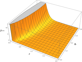
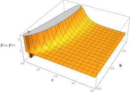
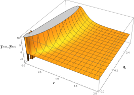
Figure 1: (color online). Plot showing the behavior of the energy conditions of the rotating spacetime for the set of values $a=0.4,b=0,\mu=1$.

Here the signatures reflect that the considered region whether it is outside the event horizon or inside the Cauchy horizon correspond to the choice $(-,+)$, respectively. The energy-momentum tensor can be expressed in terms of orthonormal basis which reads

$$T^{(a)(b)}=e_{\mu}^{(a)}e_{\mu}^{(b)}G^{\mu\nu},$$ (40)

which turned to be in a diagonal form. The computation reveals that the components of $T^{(a)(b)}$ are rather cumbersome. Therefore, we consider $\theta=0,\pi$ for the matter of simplicity. The nonzero components of $T^{(a)(b)}$ for $\theta=0,\pi$ are given as follows

$$T^{(0)(0)} = \frac{m^{\prime}(3r^{2}+a^{2})(r^{2}+b^{2})^{2}-b^{2}m^{\prime\prime}r\Delta}{2r^{3}(r^{2}+a^{2})[b^{2}m+(r^{2}+a^{2})(r^{2}+b^{2})]},$$

$$T^{(1)(1)} = -\frac{m^{\prime}(3r^{2}+a^{2})}{2r(r^{2}+a^{2})^{2}},$$

$$T^{(2)(2)} = -\frac{m^{\prime\prime}r(r^{2}+a^{2})+2m^{\prime}a^{2}}{2r(r^{2}+a^{2})^{2}},$$

$$T^{(3)(3)} = -\frac{m^{\prime\prime}r(r^{2}+a^{2})+2m^{\prime}a^{2}}{2r(r^{2}+a^{2})^{2}},$$

$$T^{(4)(4)} = -\frac{m^{\prime\prime}(r^{2}+a^{2})^{2}(r^{2}+b^{2})^{2}-m^{\prime}b^{2}(3r^{2}+a^{2})\Delta}{2r^{3}(r^{2}+a^{2})^{2}[b^{2}m+(r^{2}+a^{2})(r^{2}+b^{2})]}.$$ (41)

As can be seen from the components of energy-momentum tensor that for both $T^{(0)(0)}$ and $T^{(4)(4)}$ components, there is a dependence on both angular momenta. If we set $b=0$ in (IV), it turns out that $T^{(0)(0)}=-T^{(1)(1)}$. The typical behavior of the energy conditions can be seen from the Fig 1. We see that there is a violation of weak energy condition in $T^{(0)(0)}+T^{(4)(4)}$, but only by a small amount (cf. Fig 1). It is the black hole rotation which leads to the violation of energy condition for any physically reasonable mass. The violation of weak energy condition cannot be prevented in the rotating regular black holes Bambi:2013ufa ; Neves:2014aba . Now we are going to discuss some important properties of the rotating spacetime in next section.

V Nature of rotating spacetimes

In this section, we discuss some important properties of the rotating five-dimensional electrically charged Bardeen regular spacetime comprehensibly.

V.1 Curvature invariants

We calculate the curvature invariants of the rotating five-dimensional electrically charged Bardeen regular spacetime (30) to verify the regularity of them. In order to do so we compute the expressions of the curvature scalars and find their limiting values. At first we compute the Ricci scalar which takes the form

$$R = g^{\mu\nu}R_{\mu\nu}=R^{\mu}_{\mu}=\frac{m^{\prime\prime}r+2m^{\prime}}{r\rho^{2}},$$ (42)

where $m$ is the mass function defined in (25) and prime (^′) denotes the derivative with respect to the radial coordinate $r$. The other curvature scalar which is contraction of the Ricci tensor is given by

$$\mathcal{R} = R_{\mu\nu}R^{\mu\nu}=\frac{\rho^{4}m^{\prime\prime 2}r^{2}+2m^{\prime}m^{\prime\prime}\rho^{2}(\rho^{2}-2r^{2})r+m^{\prime 2}(3\rho^{4}-4\rho^{2}r^{2}+7r^{4})}{2r^{2}\rho^{8}}.$$ (43)

Another important curvature scalar known as the Kretschmann scalar $(K=R_{\mu\nu\gamma\delta}R^{\mu\nu\gamma\delta})$ can be computed as follows

$$K = \frac{\left[\rho^{8}m^{\prime\prime 2}-4\rho^{4}\left(2\rho^{2}m^{\prime}r+\gamma m\right)m^{\prime\prime}+24\gamma\alpha m^{2}\right]r^{2}-8\rho^{2}\xi mm^{\prime}r+2\rho^{4}\delta m^{\prime 2}}{r^{2}\rho^{12}},$$ (44)

where $\gamma=\rho^{2}-4r^{2}$, $\delta=\rho^{4}-6\rho^{2}r^{2}+16r^{4}$, and $\xi=\rho^{4}-16\rho^{2}r^{2}+24r^{4}$. We further compute the Weyl invariant ($W1R=C_{\mu\nu\gamma\delta}C^{\mu\nu\gamma\delta}/8$) for the spacetime (30), which is given by

$$W1R = \frac{\left(11\rho^{8}m^{\prime\prime 2}+432\gamma\eta m^{2}-72\rho^{4}\gamma mm^{\prime\prime}\right)r^{2}-2\rho^{2}\left(\rho^{4}\lambda m^{\prime\prime}+72\xi m\right)m^{\prime}r+\rho^{4}\sigma m^{\prime 2}}{144r^{2}\rho^{12}},$$

where $\eta=3\rho^{2}-4r^{2}$, $\lambda=5\rho^{2}+54r^{2}$, and $\sigma=17\rho^{4}-180\rho^{2}r^{2}+504r^{4}$. It is noticeable that the curvature invariants of the rotating five-dimensional electrically charged Bardeen regular black holes have very tedious mathematical expressions. Therefore, it is bit difficult to visualize analytically the nature of them. For this reason, we plot the curvature invariants and the illustration of these invariants can be seen in Fig. 2. This illustration confirms that all the curvature invariants are well behaved even at the origin $r=0$. The finiteness of scalar invariants at $r=0$ is in support of the existence of the de Sitter belt around the origin thereby the spacetime does not terminate in signaling a singular nature.

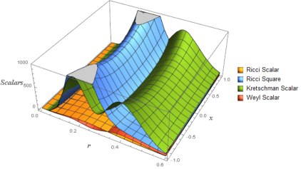
Figure 2: (color online). Plot showing the behavior of curvature invariants of the rotating spacetime for the set of values $a=0.5,b=0.6,q_{e}=0.4,\mu=1$ ($x=\cos\theta$).

Apart from the aforementioned curvature invariants, there exists other curvature invariants as well. We are also interested in calculation of trace-free Ricci invariants which can be expressed by $r_{1}=S_{\mu}^{\nu}S_{\nu}^{\mu}/4$, $r_{2}=-S_{\mu}^{\nu}S_{\nu}^{\gamma}S_{\gamma}^{\mu}/8$, and $r_{3}=S_{\mu}^{\nu}S_{\nu}^{\gamma}S_{\gamma}^{\delta}S_{\delta}^{\mu}/16$. The trace-free Ricci tensor is given by $S_{\mu\nu}=R_{\mu\nu}-Rg_{\mu\nu}/D$, where $D$ represents the number of dimensions. Hence, these trace-free Ricci invariants for the rotating spacetime (30) can be expressed in the following forms

$$r_{1} = \frac{3{m^{\prime\prime}}^{2}\rho^{4}r^{2}+2m^{\prime}m^{\prime\prime}\rho^{2}r(\rho^{2}-10r^{2})+{m^{\prime}}^{2}(7\rho^{4}-20\rho^{2}r^{2}+40r^{4})}{40\rho^{8}r^{2}},$$

$$r_{2} = \frac{3(3m^{\prime}-m^{\prime\prime}r)\left[{m^{\prime\prime}}^{2}r^{2}(\rho^{2}-r^{2})^{2}+2m^{\prime}m^{\prime\prime}\rho^{2}r(2\rho^{2}-5r^{2})-{m^{\prime}}^{2}(\rho^{4}+10\rho^{2}r^{2}-20r^{4})\right]}{800\rho^{10}r^{3}},$$

$$r_{3} = \frac{1}{16000\rho^{16}r^{4}}\Big{[}21{m^{\prime\prime}}^{4}\rho^{8}r^{4}+28m^{\prime}{m^{\prime\prime}}^{3}\rho^{6}r^{3}(\rho^{2}-10r^{2})$$ (46)

$$+6{m^{\prime}}^{2}{m^{\prime\prime}}^{2}\rho^{4}r^{2}(29\rho^{4}-100\rho^{2}r^{2}+260r^{4})-4{m^{\prime}}^{3}m^{\prime\prime}\rho^{2}r(17\rho^{6}-660\rho^{2}r^{4}+210\rho^{4}r^{2}+1000r^{6})$$

$$+{m^{\prime}}^{4}\{170r^{8}+r^{4}(\rho^{2}-r^{2})(1566\rho^{2}-2322r^{2})+(\rho^{2}-r^{2})^{3}(181\rho^{2}+23r^{2})\}\Big{]}.$$

We can easily check the limit, $r\rightarrow 0$ for the trace-free Ricci invariants which confirms that they do not diverge. This is the confirmation from these curvature invariants that the spacetime (30) is regular everywhere.

V.2 Horizon structure

Next, we discuss the horizons of the rotating five-dimensional electrically charged Bardeen regular black hole. It is noticeable that the metric (30) has a singularity at $g^{rr}=\Delta=0$, which corresponds to the horizons of the black hole. Keep in mind that this is a coordinate singularity and it can easily be removed by a particular choice of transformations. The horizons of the rotating five-dimensional electrically charged Bardeen regular black hole are solutions of the following equation

$$\left(r^{2}+a^{2}\right)\left(r^{2}+b^{2}\right)-\mu r^{2}\left(\frac{r^{3}}{r^{3}+q_{e}^{3}}\right)^{4/3}=0.$$ (47)

It is clear that the analytical solution of (47) is not easily found because of the fractional power. In order to understand the nature of (47), we plot it for different set of values of the parameters $a$, $b$, and $q_{e}$ (cf. Fig. 3). We find that there exists three different cases in horizons profile which correspond to the two horizons (blue dashed line), extremal horizons (green dashed line), and no horizon (red line). The two horizons are correspond to the event horizon and the Cauchy horizon. The extremal horizons or degenerate horizons exist for the precise values of charge $q_{e}$ (cf. Fig. 3).

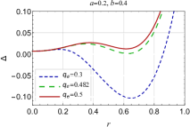
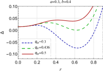
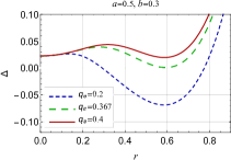
Figure 3: (color online). Plot showing the behavior of horizons of the rotating five-dimensional electrically charged Bardeen regular black holes.

The static limit surface or infinite redshift surface of the rotating five-dimensional electrically charged Bardeen regular black hole can be evaluated by equating the coefficient of $dt^{2}$ to zero, i.e.,

$$r^{2}+a^{2}\cos^{2}\theta+b^{2}\sin^{2}\theta-\mu\left(\frac{r^{3}}{r^{3}+q_{e}^{3}}\right)^{4/3}=0$$ (48)

depending on the parameters $a$, $b$, and $q_{e}$ as well as on the angle $\theta$. We show the effect of these parameters on the shape of the static limit surface in Fig. 4, by considering different sets of values of $a$, $b$, and $q_{e}$.

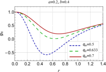
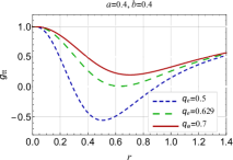
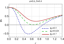
Figure 4: (color online). Plot showing the behavior of static limit surface of rotating five-dimensional electrically charged Bardeen regular black hole.

It is found that there exists three different cases which correspond to the two roots (blue dashed line), degenerate roots (green dashed line), and no root (red line). We illustrate different cases where the static limit surfaces have degenerate roots as can be seen in in Fig. 4.

V.3 Ergoregion

An ergoregion is a spacetime region where timelike Killing vector becomes spacelike. In black hole physics, there exists a very special phenomenon according to which a Killing field may be timelike in particular regions and spacelike in other regions of spacetime. Basically, this region lies outside the event horizon of the rotating black holes, i.e., $r_{sls}<r<r_{+}$, where $r_{sls}$ and $r_{+}$ corresponding to radius of the static limit surface and radius of the event horizon, respectively. On the other hand, the boundary of the ergoregion is known as the ergosphere. An ergosphere is a surface of infinite redshift because the norm of the time-translation Killing vector is zero there. Physically, this region is very important because an outside observer can go through it and return back without any resistance. Penrose stated that the existence of an ergoregion around the rotating black hole provides a way to retract energy from the black hole Penrose:1971uk . This process is generally called the Penrose process. We portrait different cases of the ergosphere by varying the values of the spin parameters $a$, $b$, and charge $q_{e}$ (cf. Fig. 5). We find that there is an increase in area of the ergoregion due to the variation of charge $q_{e}$ as well as the spin parameters $a$ and $b$. The near extremal cases of the horizons can also be seen in Fig. 5, where we precisely choose the values of the charge $q_{e}$ in such a way that the two horizons apparently nearly coinciding.

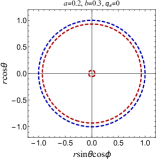
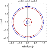
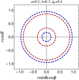
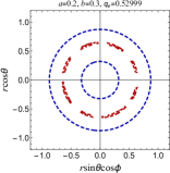
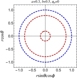
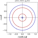
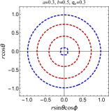
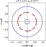
Figure 5: (color online). Plot showing the behavior of ergosphere of the rotating five-dimensional electrically charged Bardeen regular black hole.

This particular illustration can be seen in right most column of Fig. 5.

VI Black hole thermodynamics

In preceding section, we have addressed some important properties of the rotating five-dimensional electrically charged Bardeen regular black hole. Now we are going to discuss the black hole thermodynamics of this spacetime. The spacetime (30) is equipped with one timelike Killing vector, $\partial/\partial{t}$ and two rotational Killing vectors, namely, $\partial/\partial{\phi}$ and $\partial/\partial{\psi}$ corresponding to the rotations about $\phi$-axis and $\psi$-axis, respectively. The null generators at the event horizon can be determined when three of them Killing vectors are combined together as follows

$$\ell=\frac{\partial}{\partial t}+\Omega_{\phi}\frac{\partial}{\partial\phi}+\Omega_{\psi}\frac{\partial}{\partial\psi},$$ (49)

where $\Omega_{\phi}$ and $\Omega_{\psi}$ are the angular velocities of the spacetime corresponding to the $\phi$-axis and $\psi$-axis, respectively. Since $\ell$ becomes null on the event horizon at $r=r_{+}$ that leads to $\Delta(r_{H})=0$, where $r_{H}=\{r_{-},r_{+}\}$ represents both the Cauchy horizon ($r_{-}$) and the event horizon ($r_{+}$) of the black holes. The angular velocities at the event horizon are given by

$$\Omega_{\phi}=\frac{a(r_{+}^{2}+b^{2})}{(r_{+}^{2}+a^{2})(r_{+}^{2}+b^{2})},\quad\Omega_{\psi}=\frac{b(r_{+}^{2}+a^{2})}{(r_{+}^{2}+a^{2})(r_{+}^{2}+b^{2})}.$$ (50)

The mass of the rotating five-dimensional electrically charged Bardeen regular black holes can be computed as follows

$$M_{+}=\frac{(r_{+}^{2}+a^{2})(r_{+}^{2}+b^{2})(r_{+}^{3}+q_{e}^{3})^{4/3}}{r_{+}^{6}}.$$ (51)

Figure 6 depicts the behavior of the horizon radius with the mass parameter for different values of the charge $q_{e}$, and the rotation parameters $a$ and $b$. It is clear that the two horizons coincides at $r_{-}=r_{+}=r_{E}$, corresponding to the extreme black hole configuration.

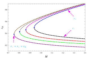
Figure 6: (color online). Plot showing the behavior of Cauchy horizon ($r_{-}$) and event horizon ($r_{+}$) of the rotating five-dimensional electrically charged Bardeen regular black hole.

We further compute the Hawking temperature of the rotating five-dimensional electrically charged Bardeen regular black holes. The spacetime (30) admits Killing field given in Eq. (49) and correspondingly we have a conserved quantity associated with it. It is possible to construct a conserved quantity by using the Killing field such that

$$\nabla^{\nu}\left(\ell^{\mu}\ell_{\mu}\right)=-2\kappa\ell^{\nu},$$ (52)

which in turn yields

$$\kappa=\sqrt{-\frac{1}{2}\nabla_{\mu}\ell_{\nu}\nabla^{\mu}\ell^{\nu}}.$$ (53)

Here $\nabla^{\nu}$ represent covariant derivative and $\kappa$ is constant along the $\ell^{\mu}$ orbits which leads to the vanishing of Lie derivative of $\kappa$ along $\ell^{\mu}$, i.e., $\mathcal{L_{\ell}}\kappa=0$. $\kappa$ is also known as the surface gravity which is proven to be constant over the event horizon. We can easily compute the surface gravity

$$\kappa=\frac{r_{+}^{7}-q_{e}^{3}r_{+}^{4}-a^{2}b^{2}r_{+}^{3}-2(a^{2}+b^{2})q_{e}^{3}r_{+}^{2}-3a^{2}b^{2}q_{e}^{3}}{r_{+}(r_{+}^{2}+a^{2})(r_{+}^{2}+b^{2})(r_{+}^{3}+q_{e}^{3})},$$ (54)

The surface gravity is related to the Hawking temperature of the black holes via $T_{+}=\kappa/2\pi$. Hence, the Hawking temperature of the rotating five-dimensional electrically charged Bardeen regular black holes is given by

$$T_{+}=\frac{r_{+}^{7}-q_{e}^{3}r_{+}^{4}-a^{2}b^{2}r_{+}^{3}-2(a^{2}+b^{2})q_{e}^{3}r_{+}^{2}-3a^{2}b^{2}q_{e}^{3}}{2\pi r_{+}(r_{+}^{2}+a^{2})(r_{+}^{2}+b^{2})(r_{+}^{3}+q_{e}^{3})}.$$ (55)

The black holes emit radiation when heated to the Hawking temperature. It is noticeable that equation (55) contains the Hawking temperatures for Meyers-Perry spacetime when $q_{e}=0$, the five-dimensional electrically charged Bardeen regular spacetime when $a=b=0$, and the Schwarzschild-Tagherlini spacetime when $q_{e}=a=b=0$ as special cases. The Hawking temperature does not diverge except for the $q_{e}=a=b=0$ special case and shows a finite peak (cf. Fig. 7). The typical behavior of the Hawking temperature as a function of the event horizon radius is depicted in Fig. 7 for different values of the charge $q_{e}$, and the rotation parameters $a$ and $b$. These figures suggest that the regular black holes ($q_{e}\neq 0$) are colder than the singular black holes ($q_{e}=0$). The Hawking temperature of the Schwarzshild-Tangherlini spacetime ($T_{+}=1/2\pi r_{+}$) shows the divergent behavior as $r_{+}\rightarrow 0$.

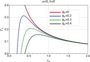
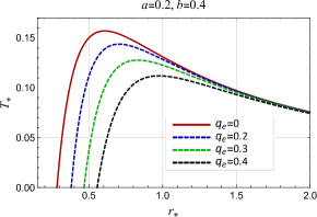
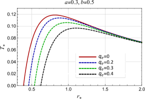
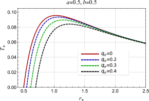
Figure 7: (color online) Plot showing the behavior of Hawking temperature ($T_{+}$) vs event horizon radius ($r_{+}$) for rotating rotating five-dimensional electrically charged Bardeen regular black holes.

Now the heat capacity of a black holes can be evaluated by using the following standard definition

$$C_{+}=\left(\frac{\partial M_{+}}{\partial r_{+}}\right)\left(\frac{\partial r_{+}}{\partial T_{+}}\right).$$ (56)

On using (51) and (55) in (56), the heat capacity for five-dimensional electrically charged Bardeen regular black holes turns out to be

$$C_{+}=\frac{4\pi(r_{+}^{2}+a^{2})^{2}(r_{+}^{2}+b^{2})^{2}(r_{+}^{3}+q_{e}^{3})^{7/3}\{r_{+}^{7}-q_{e}^{3}r_{+}^{4}-a^{2}b^{2}r_{+}^{3}-2(a^{2}+b^{2})q_{e}^{3}r_{+}^{2}-3a^{2}b^{2}q_{e}^{3}\}}{r_{+}^{5}\{a^{4}b^{4}W+2q_{e}^{3}r_{+}^{4}(a^{4}+b^{4})(4r_{+}^{3}+q_{e}^{3})+8a^{2}b^{2}r_{+}^{4}X+r_{+}^{2}(r_{+}^{2}+a^{2})Y+r_{+}^{8}Z\}},$$

where $W$, $X$, $Y$, and $Z$ are defined as follows

$$W = r_{+}^{6}+10q_{e}^{3}r_{+}^{3}+3q_{e}^{6},\quad X=r_{+}^{6}+6q_{e}^{3}r_{+}^{3}+2q_{e}^{6},$$

$$Y = r_{+}^{10}+18q_{e}^{3}r_{+}^{7}+3a^{2}b^{2}r_{+}^{6}+5q_{e}^{6}r_{+}^{4}+22a^{2}b^{2}q_{e}^{3}r_{+}^{3}+7a^{2}b^{2}q_{e}^{6},$$

$$Z = -r_{+}^{6}+6q_{e}^{3}r_{+}^{3}+q_{e}^{6}.$$ (58)

The expression has very complicated form which cannot be understand analytically. In order to see the nature of heat capacity, it will be convenient to plot the heat capacity versus event horizon radius by varying the charge $q_{e}$ as well as the rotation parameters (cf. Fig. 8).

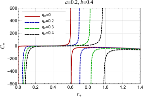
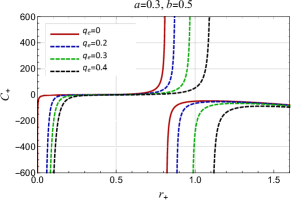
Figure 8: (color online) Plot showing the behavior of heat capacity ($C_{+}$) vs event horizon radius ($r_{+}$) for rotating five-dimensional electrically charged Bardeen regular Bardeen black holes.

This is clear from Fig. 8 that it is always possible for a suitable choice of the parameters to obtain the thermodynamically stable black holes. Figure 8 reveals that there exists phase transitions in heat capacity. The heat capacity has two branches: i) the negative branch corresponds to the unstable phase, and ii) the positive branch corresponds to the stable phase for a suitable choice of the physical parameters.

VII Conclusion

In this paper, we have discussed five-dimensional electrically charged Bardeen regular black holes spacetime by considering the coupling of nonlinear electrodynamics to general relativity. We have shown that the curvature invariants of the spacetime are not diverging at the origin ($r=0$) which indicates the regular behaviour of spacetime. Moreover, we have derived the rotating five-dimensional electrically charged Bardeen regular black hole spacetime by applying the Giampieri algorithm on the static five-dimensional electrically charged Bardeen regular spacetime. The Giampieri approach is much simpler than the NJA, since there is no need to do such tedious calculations. The rotating spacetime contains two distinct spin parameters $a$ and $b$ as well as a charge $q_{e}$ that provides a deviation, and differs it from the standard Myers-Perry spacetime. When we switch off the charge $q_{e}$, it reduces into the Myers-Perry black hole. In order to check the validity of the rotating spacetime, we have determined the nonlinear electrodynamics source. We have also computed the orthonormal basis by considering the locally nonrotating frames. By using these orthonormal basis, we have derived the components of the energy-momentum tensor, eventually discussed the energy conditions. We have discovered that there is violation of the weak energy condition in the rotating spacetime, but by a small amount.

A study of the different curvature invariants for the rotating spacetime reveals that it does not contain any spacetime singularity within it. One should note that the spacetime singularity has been removed from the spacetime through the nonlinear electrodynamics. This confirmation encourages us to study other properties of the spacetime. Therefore, the structures of the horizons, the static limit surfaces, and the ergosphere have been analysed in detail. While the horizons of the rotating spacetime are concerned, we have shown that there exists three different cases of particular interest, viz., two distinct roots corresponding to inner (Cauchy) horizon and outer (event) horizon, extremal configuration with degenerate horizons, and no root corresponding to no black hole solution. On a discussion regarding the ergosphere of the rotating five-dimensional electrically charged Bardeen regular spacetime, it has been found that the ergoregion increases with an increase in the magnitude of charge $q_{e}$ as well as spin parameters $a$ and $b$. We have further explored the thermodynamical behavior of the rotating five-dimensional electrically charged Bardeen regular spacetime by computing the Hawking temperature and the heat capacity. It has been found that there occurs phase transitions in heat capacity. In future work, we shall explore the phase space thermodynamics and critical behaviors, and critical exponents of the electrically charged Bardeen regular black holes.

- (1) T. Padmanabhan, Astrophys. Space Sci. 285, 407 (2003).
- (2) K. Schwarzschild, Sitzber. Deut. Akad. Wiss. Berlin, 3, 189 (1916).
- (3) H. Reissner, Ann. Phys. 355, 106 (1916).
- (4) B. P. Abbott et al. (LIGO Scientific Collaboration and Virgo Collaboration), Phys. Rev. Lett. 116, 061102 (2016).
- (5) B. P. Abbott et al. (LIGO Scientific Collaboration and Virgo Collaboration), Phys. Rev. Lett. 116, 241103 (2016).
- (6) B. P. Abbott et al. (LIGO Scientific Collaboration and Virgo Collaboration), Phys. Rev. X 6, 041015 (2016).
- (7) K. Akiyama et al. [Event Horizon Telescope Collaboration], Astrophys. J. 875, L5 (2019).
- (8) K. Akiyama et al. [Event Horizon Telescope Collaboration], Astrophys. J. 875, L6 (2019).
- (9) R. P. Kerr, Phys. Rev. Lett. 11, 237 (1963).
- (10) E. T. Newman and A. I. Janis, J. Math. Phys. 6, 915 (1965).
- (11) E. T. Newman, R. Couch, K. Chinnapared, A. Exton, A. Prakash and R. Torrence, J. Math. Phys. 6, 918 (1965).
- (12) M. Demianski and E. T. Newman, Bull. Acad. Polon. Sci. 14, 653 (1966).
- (13) M. Demianski, Phys. Lett. A 42, 157 (1972).
- (14) L. Herrera and J. Jiménez, J. Math. Phys. 23, 2339 (1982).
- (15) H. Kim, Phys. Rev. D 59, 064002 (1999).
- (16) S. Yazadjiev, Gen. Rel. Grav. 32, 2345 (2000).
- (17) H. Erbin, Universe 3, 19 (2017).
- (18) S. P. Drake and R. Turolla, Class. Quant. Grav. 14, 1883 (1997)
- (19) G. Clement, Phys. Rev. D 57, 4885 (1998).
- (20) S. P. Drake and P. Szekeres, Gen. Rel. Grav. 32, 445 (2000).
- (21) E. N. Glass and J. P. Krisch, Class. Quant. Grav. 21, 5543 (2004).
- (22) G. W. Gibbons, H. Lu, D. N. Page and C. N. Pope, J. Geom. Phys. 53, 49 (2005).
- (23) H. S. Kim, J. Korean Phys. Soc. 61, 313 (2012).
- (24) M. Murenbeeld and J. R. Trollope, Phys. Rev. D 1, 3220 (1970).
- (25) G. Giampieri, Gravity Research Foundation (1990).
- (26) H. Erbin and L. Heurtier, Class. Quant. Grav. 32, 165004 (2015).
- (27) Z. Mirzaiyan, B. Mirza and E. Sharifian, Ann. Phys. 389, 11 (2018).
- (28) R. C. Myers and M. J. Perry, Ann. Phys. 172, 304 (1986).
- (29) X. Dianyan, Class. Quant. Grav. 5, 871 (1988).
- (30) A. D. Sakharov, Sov. Phys. JETP, 22, 241 (1966).
- (31) J. Bardeen, in Proceedings of GR5 (Tiflis, U.S.S.R., 1968).
- (32) E. Ayón-Beato and A. García, Phys. Lett. B 493, 149 (2000).
- (33) C. Bambi and L. Modesto, Phys. Lett. B 721, 329 (2013).
- (34) E. Ayón-Beato and A. García, Phys. Rev. Lett. 80, 5056 (1998).
- (35) E. Ayón-Beato and A. García, Gen. Rel. Grav. 31, 629 (1999)
- (36) I. Dymnikova, Class. Quant. Grav. 21, 4417 (2004)
- (37) K. A. Bronnikov, Phys. Rev. D 63, 044005 (2001)
- (38) S. Shankaranarayanan and N. Dadhich, Int. J. Mod. Phys. D 13, 1095 (2004).
- (39) S. A. Hayward, Phys. Rev. Lett. 96, 031103 (2006).
- (40) H. Culetu, Int. J. Theor. Phys. 54, 2855 (2015).
- (41) L. Balart and E. C. Vagenas, Phys. Rev. D 90, 124045 (2014).
- (42) B. Toshmatov, B. Ahmedov, A. Abdujabbarov and Z. Stuchlik, Phys. Rev. D 89, 104017 (2014)
- (43) S. G. Ghosh and S. D. Maharaj, Eur. Phys. J. C 75, 7 (2015).
- (44) J. C. S. Neves and A. Saa, Phys. Lett. B 734, 44 (2014).
- (45) M. Azreg-Aïnou, Phys. Lett. B 730, 95 (2014)
- (46) M. Azreg-Aïnou, Phys. Rev. D 90, 064041 (2014).
- (47) S. G. Ghosh, Eur. Phys. J. C 75, 532 (2015).
- (48) M. S. Ali and S. G. Ghosh, Phys. Rev. D 98, 084025 (2018).
- (49) S. G. Ghosh, D. V. Singh and S. D. Maharaj, Phys. Rev. D 97, 104050 (2018).
- (50) A. Kumar, D. Veer Singh and S. G. Ghosh, Eur. Phys. J. C 79, 275 (2019).
- (51) M. E. Rodrigues and M. V. d. S. Silva, J. Cosmol. Astropart. Phys. 1806, 025 (2018).
- (52) A. N. Aliev and V. P. Frolov, Phys. Rev. D 69, 084022 (2004).
- (53) R. Penrose and R. M. Floyd, Nature (London) 229, 177 (1971).