A higher-dimensional generalization of the Lozi map: Bifurcations and dynamics

Abstract

We generalize the two dimensional Lozi map in order to systematically obtain piece–wise continuous maps in three and higher dimensions. Similar to higher-dimensional generalizations of the related Hénon map, these higher-dimensional Lozi maps support hyperchaotic dynamics. We carry out a bifurcation analysis and investigate the dynamics through both numerical and analytical means. The analysis is extended to a sequence of approximations that smooth the discontinuity in the Lozi map.

I Introduction

The behavior of low-dimensional nonlinear iterative maps and flows has been extensively studied and characterized over the past few decades, particularly with reference to the creation of chaotic dynamics May76 ; Yorke75 ; Henon76 ; Lozi78 . The various scenarios or routes to chaos in such systems are by now fairly well known May76 ; Arnold65 ; Newhouse78 ; Rand82 . Similar exploration of the properties of higher dimensional dynamical systems—for instance the dynamics of attractors with more than one positive Lyapunov exponent and the bifurcations through which they have been created—has not been studied in as much detail even in relatively simple systems Lozi78 ; Sprott06 ; Albers06 ; Baier90 ; Elhadjbook14 .

Linear and piecewise-linear mappings are among the simplest examples of iterative dynamical systems. The so–called Lozi map Lozi78 is analogous to the quadratic Hénon mapping Henon76 but has the advantage that more extensive analysis is possible SCOR11 . The mapping itself is only piecewise continuous, and this introduces some additional features that need to be understood more clearly bernardobook ; Simpson08 ; Simpson12 ; Kuznetsovbook . Indeed, specific bifurcation phenomenon such as border collision bifurcations can only occur in piecewise smooth dynamical systems Simpson12 ; bernardobook .

Our interest in the present paper is the generalization of the Lozi map to higher dimensions. One motivation is to compare this piecewise continuous system to a similar high-dimensional Hénon mapping SBRR13 . Of the different ways in which this can be done, we choose to extend the map to $d$–dimensions by incorporating time-delay feedback while ensuring that the system remains an endomorphism in the absence of dissipation. The dissipation is introduced at the $k$th step, $k<d$, and this also ensures that the map is a diffeomorphism. The system can therefore have $k$–positive Lyapunov exponents, and we examine the transition to high-dimensional chaos as a function of parameters, characterizing the different bifurcations that can occur. An intermediate “smooth” approximation Aziz01 of the piecewise map is also investigated vis-a-vis bifurcations for comparison.

In the next Section, the generalized Lozi map is described and a detailed analysis of the local bifurcations of the elementary fixed points is presented. The emergence of chaotic and hyperchaotic attractors and the global bifurcations that arise are discussed in Section III. Section IV is devoted to the analysis of smooth approximations to the map. The paper concludes with a discussion and summary in Section V.

II The generalized Lozi map

The two dimensional Lozi map Lozi78 is given by

$$x_{n+1} = 1-(1-\nu)y_{n}-a|x_{n}|$$

$$y_{n+1} = x_{n}\;.$$ (1)

This map is a modification of the quadratic Hénon mapping, with the parameters $\nu$ and $a$ tuning the dissipation and nonlinearity respectively. Since the map is piecewise linear, it lends itself to extensive analysis, some of which has been recently summarized Elhadjbook14 .

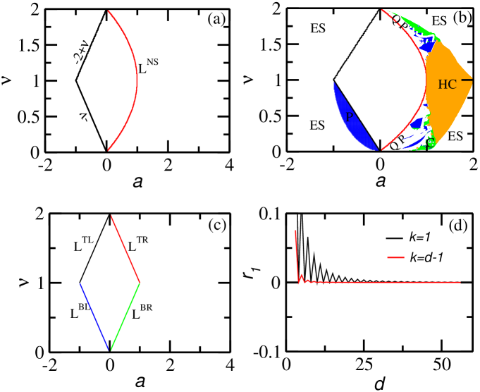
Figure 1: (a) Region of period–1 dynamics for $d$=3, $k$=2; see Eq.(II.2). (b)The organization of $a$–$\nu$ plane into unbounded dynamics (ES) and bounded dynamics: hyperchaotic (HC,orange), chaotic (C, green), periodic (P,blue). White regions sandwiched between period one dynamics and hyperchaotic/chaotic/periodic corresponds to quasiperiodic dynamics (QP). The blue regions indicate that supercritical bifurcations are possible on either side of the period one boundaries (see Fig. 2). (c) The region of period one dynamics converges asymptotically (i.e. for $d\rightarrow\infty$) and is contained within the curves $L^{TL},L^{TR},L^{BL},L^{BR}$. (d) The convergence to the curves TR,BL,BR is captured by the distance $r_{1}$ of the largest root from the unit circle as a function of dimension $d$ on these curves. $L^{NS}$ indicates the Neimark–Sacker boundary, and the other labels $L^{TR}$, $L^{TL}$, $L^{BR}$ and $L^{BL}$ are short for top left,right, and bottom left,right.

Rewriting the above as a difference delay equation, one has

$$x_{n} = 1-a|x_{n-1}|-(1-\nu)x_{n-2},$$ (2)

which suggests a natural generalization to higher dimensions,

$$x_{n} = 1-a|x_{n-k}|-(1-\nu)x_{n-d}.$$ (3)

Here $d$ and $k$ are integers such that $k<d$, and we take $0\leq\nu\leq 2$. The mapping is conservative when $\nu$ is 0 or 2, and is dissipative otherwise. For $\nu=1$ the map reduces to a $k$–dimensional endomorphism, while for $\nu\neq 1$ the map is a $d$–dimensional diffeomorphism. In the next subsection we analyze the implications of different choices of $d$ and $k$ for this map.

II.1 The base maps and $q$–degeneracy

The integers $d$ and $k$ are either co-prime or share a common factor $q$. When $k$ and $d$ have a common factor $q$, it is easy to see that all the eigenvalues of the Jacobian are $q$–fold degenerate, and this leads to a $q$–fold degeneracy in the Lyapunov exponents. It therefore suffices to examine the case of $d,k$ co–prime since these form the base for all other values of $k<d$, and it suffices to consider only base-maps as can be seen by the following argument. For the $n=qm$th iterate, the substitution $x_{q\cdot}$ by $\xi_{\cdot}$ gives

$$x_{qm} = 1-a|x_{qm-qk^{\prime}}|-(1-\nu)x_{qm-qd^{\prime}}$$

$$\downarrow$$

$$\xi_{m} = 1-a|\xi_{m-k^{\prime}}|-(1-\nu)\xi_{m-d^{\prime}}.$$ (4)

The maps Eq. (3) and Eq. (II.1) differ in that there are $q$ hidden variables within each $\xi_{m}$. Thus the Jacobian can be separated into $q$ identical blocks, giving rise to a $q$–degenerate $(d^{\prime},k^{\prime})$ map.

II.2 Fixed points: Stability

The delay map, Eq. (3) can be rewritten as a $d$-dimensional iteration,

$$x^{1}_{n+1} = 1-a|x^{k}_{n}|-(1-\nu)x^{d}_{n}$$

$$x^{2}_{n+1} = x^{1}_{n}$$

$$\vdots$$

$$x^{d}_{n+1} = x^{d-1}_{n}$$ (5)

The fixed points of the mapping are those for which $\{x^{1}_{n+1},\ldots,x^{d}_{n+1}\}=\{x^{1}_{n},\ldots,x^{d}_{n}\}$. Solving, we find

$$x^{1*} = x^{2*}=\dots=x^{d*}=x_{\pm}$$

$$\mathrm{with~{}~{}}x_{\pm} = \frac{1}{2-\nu\pm a}.$$ (6)

of these two fixed points, $x_{-}$ is always unstable. The matrix elements of the Jacobian of the map in Eq. (3) are given by

$$\left[\mathbf{J}\right]_{ij}=\begin{cases}1&j=i-1\;,\;\;d\;\geq\;i\;\geq\;2\\ \pm a&i=1\;,\;j=k\\ -(1-\nu)&i=1\;,\;j=d\\ 0&\mathrm{otherwise}\end{cases}\;,$$ (7)

and it is straightforward to obtain the stability conditions on the fixed point $x_{+}$ (for arbitrary $d$ and $k$) from the characteristic polynomial $P(\lambda)$,

$$P_{1,2}(\lambda) = \lambda^{d}\;\pm\;a\lambda^{d-k}+(1-\nu).$$ (8)

If the number of real roots of the polynomials $P_{1,2}$ with real part greater than +1 (or smaller than -1) is $\sigma^{+}_{1,2}$ ($\sigma^{-}_{1,2}$), then according to Feigin’s classification of border collision bifurcations in piecewise smooth maps bernardobook , a fold bifurcation occurs when $\sigma^{+}_{1}\;+\;\sigma^{+}_{2}$ is odd. If $\sigma^{-}_{1}\;+\;\sigma^{-}_{2}$ is odd, on the other hand, a flip bifurcation occurs.

The characteristic of the Neimark–Sacker bifurcation in smooth dynamical systems is that a pair of complex eigenvalues cross the unit circle. This theory has been extended to piecewise smooth maps only recently Simpson08 and although some of the features are common, there are major differences Simpson08 . We find from numerical estimation of eigenvalues of $P_{1,2}$ for the base maps that a Neimark–Sacker bifurcation occurs via a border collision if an odd number of pairs of complex eigenvalues cross the unit circle. In particular, for the base map with $d=3,k=2$ we find that period one region is bounded by the curves as shown in Fig. 1(a):

$$L^{\mathrm{fold}}(d)\;:\;a = -2+\nu$$

$$L^{\mathrm{NS}}(d=3)(\mathrm{supercritical})\;:\;a = \nu(2-\nu)\;.$$

$$L^{\mathrm{flip}}\;:\;a = -\nu\;.$$

If either of the polynomials produce their largest roots with absolute values less than one, the fixed point $x_{+}$ is stable and contributes to the period–one region in the $a$–$\nu$ parameter space, unless it hits the border $x=0$. Unlike the smooth case (i.e. the Hénon map) studied in SBRR13 the bifurcations in the Lozi map can show supercritical bifurcations on either side of the period one boundaries (of course limited upto the saddle node curve), as shown in Fig. 1(b). Since these bifurcation clearly show that orbit of the period one hits the boundary $x=0$ at such bifurcation, we attribute this distinct feature of the generalized version of the Lozi map (3) to border collision bifurcations of the map.

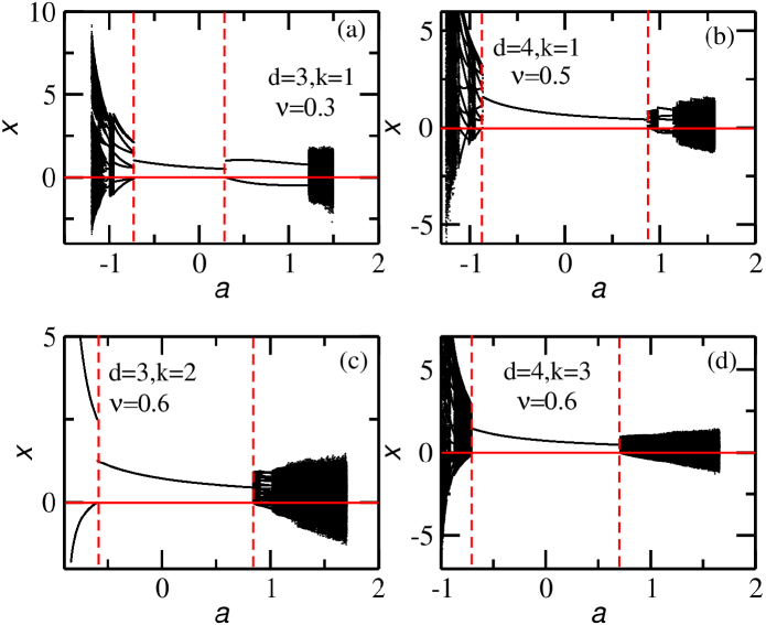
Figure 2: Bifurcation diagrams as a function of the nonlinearity $a$ for different base maps (a) $d$=3, $k$=1, $\nu$ = 0.3 (b) $d$=4, $k$=1, $\nu$=0.5, (c) $d$=3, $k$=2, $\nu$=0.6, (d) $d$=4, $k$=3, $\nu$=0.6. The boundaries of stable period-1 dynamics are indicated by dashed vertical lines; these are also the border-collision bifurcation points.

II.3 Bifurcations diagrams

Bifurcation diagram in the two dimensional $a$–$\nu$ parameter space for $d=3,k=2$ is shown in Fig. 1(b). A typical feature of $a$–$\nu$ parameter space is the existence of hyperchaotic (HC), chaotic (C), quasiperiodic (QP), and periodic regions. These features are shared by other members (with different $d$ and $k$ values) of this generalized Lozi map. Representative bifurcation diagrams as a function of $a$ for different $(d,k)$ combinations are shown in Fig. 2 and the corresponding orbital characteristics are shown via Lyapunov exponents in Fig. 3. In each case $\nu$ is different but fixed. An interesting feature of these bifurcation diagrams is that for for $0<\nu<1$ some base maps exhibit bounded non–trivial dynamics as the parameter $a$ is decreased to the left of the period one boundary. Typically these were found to be a flip bifurcation below $a<-\nu$ when $d=3,k=2$ and supercritical Neimark–Sacker type bifurcations for $d=4,k=3$. Such feature are typically of these maps even across different combination of dimensionality parameters ($d$,$k$). We should mention that such phenomenon was not found for a similarly generalized Hénon map SBRR13 , and appears to be a result of border collision bifurcations. It is important to note that the theory of bifurcations in smooth dynamical systems does not explain these features Kuznetsovbook .

III High dimensional dynamics

In this Section we examine the bifurcations starting from the period-1 fixed point as a function of nonlinearity parameter for different embedding dimensions $d$ and the endomorphism dimension $k$.

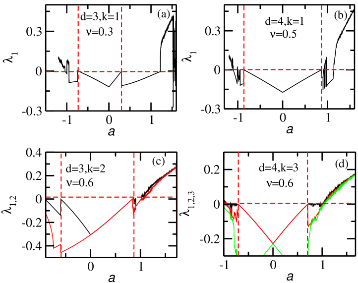
Figure 3: k- largest Lyapunov exponents for the systems corresponding to the bifurcation diagrams shown in Fig. 2 . The different base maps are (a) $d$=3, $k$=1, $\nu$=0.3, (b) $d$=4, $k$=1, $\nu$=0.5, (c) $d$=3, $k$=2, $\nu$=0.6, and (d) $d$=4, $k$=3, $\nu$=0.6. The boundaries of the stable period-1 dynamics are indicated by dashed vertical lines; the left boundary is a border collision bifurcation point.

III.1 Bounded dynamics

In the limit $d\rightarrow\infty$ period–1 motion converges to a region shown in Fig. 1(c): the boundaries are the following curves,

$$L^{TL}\>\>:\;a = -2+\nu$$

$$L^{TR}\>\>:\;a = 2-\nu$$

$$L^{BL}\>\>:\;a = -\nu$$ (9)

$$L^{BR}\>\>:\;a = \nu,$$

in the $a-\nu$ parameter space. These curves can be understood from the properties of the characteristic polynomials Eq. (8) in the limit of $d\rightarrow\infty$. The distance $r_{1}$ between the leading root of the characteristic polynomial Eq. (8) and the unit circle on the curve $L^{TL}$, in the extreme case of $k=1$ and $k=d-1$, are shown in Fig. 1(d): $r_{1}$ approaches zero as the dimension $d$ is increased. Similar behavior of $r_{1}$ is also observed on $L^{BR},L^{BL}$, $T^{LR}$ and for $1<k<d-1$.

III.2 Hyperchaos

The map Eq. (3) exhibits at most $k$ positive Lyapunov exponents as nonlinearity parameter $a$ is varied: this is due to the fact that the nonlinearity in the map occurs at the $k^{th}$ previous iteration step. The stretching and folding that is responsible for introducing sensitivity to initial conditions in the map Ottbook , occurs in $k$ directions, and this results in the maximum $k$ number of possible positive Lyapunov exponents; see Figs. 4(a)–(b). Additionally, for $\nu=1$, the map is a $k$–dimensional endomorphism (and is not invertible)

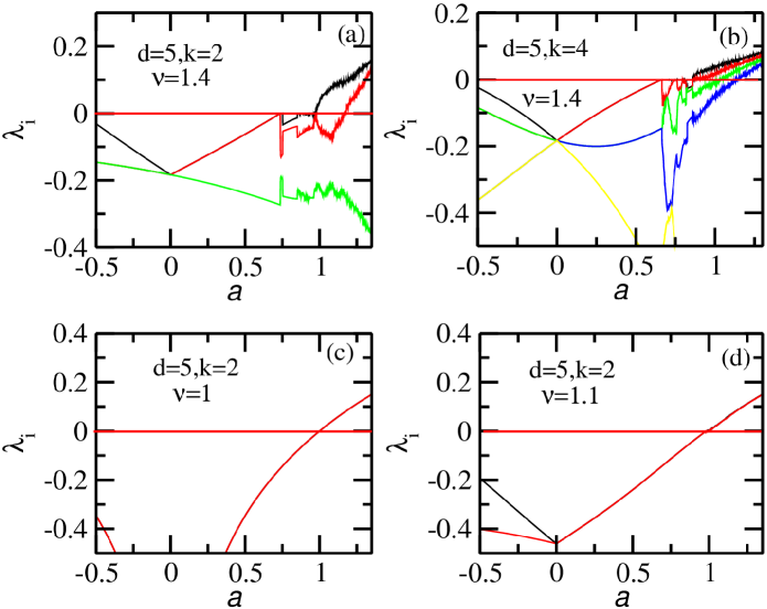
Figure 4: The Lyapunov exponent spectrum ($\lambda_{i},i=1,...,k+1$) as a function of nonlinearity parameter for $d=5$. (a)–(b) demonstrate that for a given dimension $d$ the number of positive Lyapunov exponents are governed by the parameter $k$. We keep $\nu=1.4$ and plot all the Lyapunov exponents for $k=2$ in (a) and $k=4$ in (b). (c)–(d) demonstrate the breaking of degeneracy in the Lyapunov spectrum observed in the endomorphism $\nu=1$ by making the map diffeomorphic $\nu=1.1$ (see text for explanation).

with $k$–fold degenerate Lyapunov exponents, i.e. all of these LEs are identical and become positive at the same value of the nonlinearity parameter $a$ as can be seen in Fig. 4(c). Embedding the $k$–dimensional endomorphism in a $d$–dimensional space does not change this behavior. However when the map is made diffeomorphic by enabling the contraction/dissipation parameter ($\nu\neq 1\;\&\;0\leq\nu\leq 2$) the degeneracy in the Lyapunov exponents is lifted, although the maximum possible number of positive Lyapunov exponents is still $k$ as can be seen in Fig. 4(d).

Route to chaos is observed via the quasiperiodic and also via finite period–doubling route, as seen in the Lyapunov spectra Fig. 3 and Fig. 4. The period doubling cascade terminates after a few doublings, leading to chaos. On the other hand chaos and hyperchaos transition is smooth, since the first $k$–largest Lyapunov exponents behave smoothly as they hierarchically become positive at different values of the nonlinear parameter $a$. This typically means that the map Eq. (3) can be written as a hierarchy of chaotically driven maps at subsequent transitions to higher chaos Harr00 , this is similar to the chaos hyperchaos transition in the generalized Hénon map SBRR13 .

IV Smooth approximations

In this section we analyse a smooth approximation of the generalized Lozi map (3).

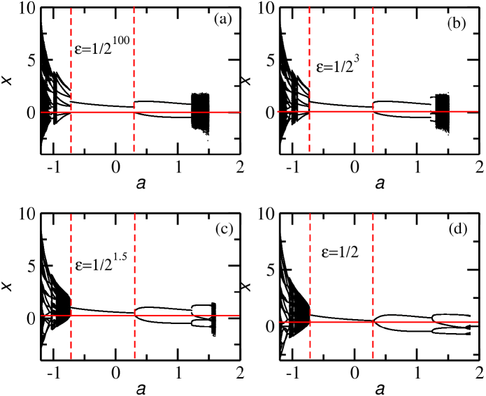
Figure 5: The bifurcation diagram for $d=3,k=1$ for different values of $\epsilon$. As $\epsilon$ is increased from (a)–(d) characteristics of smooth bifurcations emerge in the form of period doubling.

We replace the modulus function $|\cdot|$ in Eq. (3) with a smooth function $S_{\epsilon}(\cdot)$:

$$x_{n} = 1-aS_{\epsilon}(x_{n-k})-(1-\nu)x_{n-d}$$ (10)

$$S_{\epsilon}(x_{n-k}) = \begin{cases}x_{n-k}^{2}/2\epsilon+\epsilon/2&if\;\;|x_{n-k}|\leq\epsilon\\ |x_{n-k}|&if\;\;|x_{n-k}|\geq\epsilon\end{cases}\;,$$

where $0<\epsilon<1$. The function $S_{\epsilon}(x_{n-k})$ extends the smooth approximation applied to the two dimensional Lozi map Aziz01 to our high dimensional generalization of the Lozi map and removes the discontinuity in the slope at $x_{n-k}=0$.

The fixed points of the new map in Eq. (10) are given by:

$$x_{\pm} = \begin{cases}\frac{1}{2-\nu\pm\;a}&if\;\;|x|>\epsilon\\ \frac{\epsilon}{a}\Big{(}-(2-\nu)\\ \pm\sqrt{(2-\nu)^{2}+\frac{2a}{\epsilon}-a^{2}}\Big{)}&if\;\;|x|\leq\epsilon\end{cases}$$ (11)

the first set of these fixed points are similar to those of Lozi map (see Eq. (II.2)) and lose stability by colliding with one of the borders located at $\pm\epsilon$ as nonlinearity parameter $a$ is varied. The new orbits that appear following this border collision bifurcation depend on the delay parameters $d$ and $k$, although the maximum number of positive Lyapunov exponents is still limited to $k$. Assuming fixed values of the dissipation parameter and $\epsilon$, the variation in nonlinearity parameter can take iterations of the map also inside the region $|x|<\epsilon$ then subsequent bifurcations are no longer only due to border collisions: borders at $\pm\epsilon$ have well defined first derivatives and once an orbit enters the region $|x|<\epsilon$ the dynamics is also governed by the smooth approximation.

The case of $d=2$ and $k=1$ was illustrated in Aziz01 , where it was observed that the period-doubling route to chaos is achieved for finite values of $\epsilon$ (note that period doubling route to chaos is absent for $\epsilon$=0).

For $d>2$ bifurcation scenarios easily understood by writing the smoothness parameter as $\epsilon=1/2^{n_{\epsilon}},n_{\epsilon}\geq 0$. For the case of $d$=3, $k$=1 the loss of stability of the fixed point as nonlinearity parameter is varied is dependent on $n_{\epsilon}$: border collision bifurcations gives way to period doubling bifurcations as $n_{\epsilon}$ decreases (Fig. 5(a)–(d)). Similar observations are made when a Neimark–Sacker type bifurcation is involved in the Lozi map with $d=3,k=2$, where border collision bifurcations (Fig. 6(a) ) give way to smooth bifurcations Fig. 6(d).

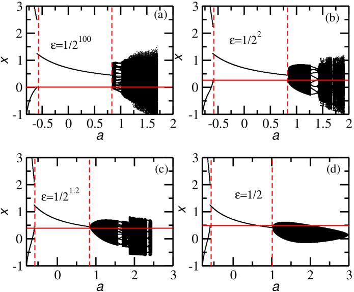
Figure 6: The bifurcation diagrams for $d=3,k=2$ for different values of $\epsilon$. As $\epsilon$ is increased from (a)–(d) characteristics of smooth bifurcations emerge in the form of period doubling. The figures (d)–(a) also indicate emergence of border collision bifurcation beginning from smooth period doubling bifurcations in (d).

In the Hénon maps the chaotic dynamics follows directly after the Neimark–Sacker bifurcation via a crisis–like transition SBRR13 . Thus the effect of $\epsilon>$ 0 is to introduce bifurcations which are a mix of border collisions and smooth bifurcations.

V Discussion and Summary

In this paper we have introduced a generalized time–delayed Lozi map with nonlinear feedback from $k$ earlier steps and linear feedback from $d$ earlier steps. This simple feedback process governs the dimensionality of the maps. The parameter $k$ ($<d$) determines the number of positive Lyapunov exponents. Further more, the family of maps formed as a result of different combinations of dimensionality parameters are classified into base maps when $d$ and $k$ are co–prime. All other maps reducible to these base maps exhibit a $q$-fold degenerate Lyapunov spectrum when $d$ and $k$ share a common factor $q$. Bifurcation analysis was performed in a limited region of the parameter space. In particular, fixed point dynamics loses stability through the fold, flip and the Neimark Sacker bifurcations via border collisions. Analytic forms were determined for these boundaries, and the flip and NS bifurcation curves were found to depend on the dimension $d$. With increasing dimension, the region of period one dynamics was found to converge in the parameter plane.

The dynamics evolves abruptly from regular to chaos due to piece-wise nature of the map. Subsequent transitions from chaos to hyperchaos, however, are smooth as indicated by Lyapunov spectrum: the dimension of the attractor changes smoothly if there are no abrupt transitions in Lyapunov spectrum Harr00 ; SBRR13 .

A smooth approximation of the map enabled the analysis of the bifurcations vis-a-vis further comparing some of the bifurcations to the generalized the Hénon map. It showed that some of the bifurcations observed persist on both the piecewise Lozi and Hénon map. Further exploration of a more general unified mapping is a project for future work. Another possible project for a future work is the analysis of conservative limit in these class of maps: orbits in the conservative limit are only possible when $d=2k$,therefore in the conservative limit hyperchaotic orbits are indeed possible with $k-$positive Lyapunov exponents. The exploration of the conservative limit of this map could be a task for future work.

References

- (1) T. Y. Lee and J. A. Yorke, Amer. Math. Monthly, 82, 985 (1975).
- (2) M. Hénon, Commun. Math. Phys. 50, 69 (1976).
- (3) R. Lozi,J. Phys. Colloq., 39, C5–9–C10 (1978).
- (4) R. M. May, Nature, 261, 459 (1976).
- (5) V. I. Arnold,Trans. Am. Math. Soc. Ser. 46, 213, (1965).
- (6) S. Newhouse, D. Ruelle, & F. Takens, Commun. Math. Phys. 64, 35 (1978).
- (7) D. Rand, S. Ostlund, J. Sethna, & E. D. Siggia, Phys. Rev. Lett. 49, 132 (1982).
- (8) J. C. Sprott, Elec. J. Theor. Phys. 3, 19 (2006).
- (9) D. J. Albers, and J. C. Sprott, Physica D 223, 194 (2006).
- (10) G. Baier and M. Klein,Phys. Lett. A 151, 281 (1990).
- (11) Z. Elhadj Lozi Mappings: Theory and Applications (CRC Press, Boca Raton, 2014).
- (12) V. Botella–Soler, J. M. Castelo, J. A. Oteo, and J. Ros, J. Phys. A: Math. Theor., 44, 305101 (2011).
- (13) M. A. Aziz–Alaoui,C. Robert, and C. Grebogi,Chaos Soliton & Fractal 12, 2323 (2001)
- (14) M. di Bernardo, C. J. Budd, A. R. Chumpney, and P. Kowalczyk,Piecewise–smooth Dynamical Systems:Theory and Applications (Springer–Verlag, London 2008).
- (15) D. J. W. Simpson and J. D. Meiss, SIAM J. Appl. Dyn. Sys. 7, 795 (2008).
- (16) S. Bilal and R. Ramaswamy, Int. J. Bif. Chaos 23, 1350045 (2013).
- (17) Y. A. Kuznetsov, Elements of Applied Bifurcation Theory (2/e), (Springer Verlag, Berlin).
- (18) E. Ott, Chaos in Dynamical Systems (Cambridge University Press 1993).
- (19) K. T. Alligood, T. D. Sauer, and J.A. Yorke, Chaos: An Introduction to Dynamical Systems (Springer-Verlag, New York 2000).
- (20) M. A. Harrison and Y-C. Lai, Int. J. Bif. Chaos 10, 1471 (2000).
- (21) D. J. W. Simpson and J. D. Meiss, Physica D 241, 1861 (2012).