Ensemble Learning of Coarse-Grained Molecular Dynamics Force Fields with a Kernel Approach

Abstract

Gradient-domain machine learning (GDML) is an accurate and efficient approach to learn a molecular potential and associated force field based on the kernel ridge regression algorithm. Here, we demonstrate its application to learn an effective coarse-grained (CG) model from all-atom simulation data in a sample efficient manner. The coarse-grained force field is learned by following the thermodynamic consistency principle, here by minimizing the error between the predicted coarse-grained force and the all-atom mean force in the coarse-grained coordinates. Solving this problem by GDML directly is impossible because coarse-graining requires averaging over many training data points, resulting in impractical memory requirements for storing the kernel matrices. In this work, we propose a data-efficient and memory-saving alternative. Using ensemble learning and stratified sampling, we propose a 2-layer training scheme that enables GDML to learn an effective coarse-grained model. We illustrate our method on a simple biomolecular system, alanine dipeptide, by reconstructing the free energy landscape of a coarse-grained variant of this molecule. Our novel GDML training scheme yields a smaller free energy error than neural networks when the training set is small, and a comparably high accuracy when the training set is sufficiently large.

I Introduction

Molecular dynamics (MD) simulations have become an important tool to characterize the microscopic behavior of chemical systems. Recent advances in hardware and software allow significant extensions of the simulation timescales to study biologically relevant processes (LindorffLarsenEtAl_Science11_AntonFolding, ; BuchEtAl_JCIM10_GPUgrid, ; ShirtsPande_Science2000_FoldingAtHome, ). For example, we can now characterize the configurational changes, folding and binding behavior of small to intermediate-sized proteins through MD on the timescale of milliseconds to seconds (DrorEtAl_PNAS11_DrugBindingGPCR, ; ShuklaPande_NatCommun14_SrcKinase, ; PlattnerNoe_NatComm15_TrypsinPlasticity, ; PlattnerEtAl_NatChem17_BarBar, ; PaulEtAl_PNAS17_Mdm2PMI, ; NoeAnnRev2020, ). However, the computational complexity of evaluating the potential energy prohibits this approach to scale up to significantly larger systems and/or longer timescales. Therefore, multiple ways have been proposed to speed up atomistic simulations, such as advanced sampling methods (e.g., umbrella sampling (Frenke2001un, ; Torrie1977, ; Johannes2011, ), parallel tempering (Swendsen1986, ; Neal1996, )) or adaptive sampling (Rajamani_Proteins24_1775, ; PretoClementi_PCCP14_AdaptiveSampling, ; BowmanEnsignPande_JCTC2010_AdaptiveSampling, ). An alternative approach is to reduce the dimensionality of the system by coarse-graining (CG) (ClementiCOSB, ; Davtyan2012, ; Izvekov2005, ; Marrink2004, ; MllerPlathe2002, ; Noid2013, ). The fact that macromolecules usually exhibit robust collective behavior suggests that not every single degree of freedom is per se essential in determining the important macromolecular processes over long timescales. Furthermore, a CG representation of the system simplifies the model and allows for a more straightforward physico-chemical interpretation of large-scale conformational changes such as protein folding or protein-protein binding(ClementiCOSB, ).

Once the mapping from the atomistic to the CG representation is defined, a fundamental challenge is the definition of an effective potential in reduced coordinates, such that the essential physical properties of the system under consideration are retained. The choice of the relevant properties crucially dictates the definition of the CG model.

Following a top-down approach, the CG procedure is driven by the objective to reproduce macroscopic properties, such as structural information or experimentally measured observables (Nielsen2003, ; MatysiakClementi_JMB04_Perturbation, ; MatysiakClementi_JMB06_Perturbation, ; Marrink2004, ; Davtyan2012, ; Chen2018, ). In a bottom-up approach, on the other hand, an effective potential is designed to reproduce a selection of properties of an atomistic model, for instance the probability distribution in a suitable space and the corresponding metastable states (Lyubartsev1995, ; MllerPlathe2002, ; Praprotnik2008, ; Izvekov2005, ; Wang2009, ; Shell2008, ).

In the past several years, machine learning (ML) techniques have been increasingly applied in molecular simulation (noe2019science, ; NOE202077, ; NoeAnnRev2020, ; Schutt2019, ). Bottom-up CG methods have also started to leverage the advances in ML, to define classical atomistic potentials or force fields from quantum chemical calculations (BehlerParrinello_PRL07_NeuralNetwork, ; Bartok2010, ; Rupp2012, ; Bartok2013, ; Smith2017, ; Bartok2017, ; Schuett2017, ; Smith2018, ; Schuett2018, ; Grisafi2018, ; Imbalzano2018, ; Nguyen2018, ; ZhangHan2018, ; ZhangHan2018_PRL, ; BereauEtAl_JCP18_Physical, ; ChmielaEtAl_SciAdv17_EnergyConserving, ; ChmielaEtAl_NatComm18_TowardExact, ), to learn kinetic models (MardtEtAl_VAMPnets, ; WuEtAl_NIPS18_DeepGenMSM, ; WehmeyerNoe_TAE, ; HernandezPande_VariationalDynamicsEncoder, ; RibeiroTiwary_JCP18_RAVE, ), or to design effective CG potential from atomistic simulations (John2017, ; ZhangHan2018_CG, ; wang2019, ). In this context, we have recently shown that a deep neural network (NN) can be used in combination with the well established “force matching” approach (Noid2008, ) to define a coarse-grained implicit water potential that is able to reproduce the correct folding/unfolding process of a small protein from atomistic simulations in explicit water (wang2019, ). In the force matching approach, the effective energy function of the CG model is optimized variationally, by finding the CG force field that minimizes the difference with the instantaneous atomistic forces projected on the CG coordinates. As there are multiple atomistic configurations consistent with a CG configuration, this estimator is very noisy and this approach requires a large amount of training data. It is thus restricted to parametric models like NNs, as the computational complexity of non-parametric models is directly linked to training set size. Here we propose a method to overcome this limitation in the dataset via bootstrap aggregation in combination with a non-parametric, kernel-based regressor.

In particular, we use the Gradient-Domain Machine Learning (GDML) approach (ChmielaEtAl_SciAdv17_EnergyConserving, ; CHMIELA201938, ). In the application to quantum data, GDML is able to use a small number (usually less than a few thousands) of example points to build an accurate force field for a specific molecule. Because of the degeneracy of the mapping, the training data required to reconstruct a coarse-grained force field is much larger, and the fact that memory requirements scale quadratically with data set size prevents a direct application of GDML to the definition of CG models.

To solve this problem, we pursue a hierarchical ensemble learning approach in which the full training set is first divided into smaller batches that are trained independently. A second GDML layer is then applied to the mean prediction of this ensemble, providing the second model with a consistent set of inputs and outputs. We show that GDML with ensemble learning can be efficiently used for the coarse-graining of molecular systems.

The structure of the paper is as follows. In the section “Theory And Methods”, we briefly review the principle of force matching that we use for coarse graining, as well as mathematical underpinnings of the kernel ridge regression used in the GDML method. Then we describe the idea of ensemble learning, and explain how it solves the problem associated with the large number of training points required by force matching. In the “Results” section, we demonstrate that a GDML approach trained with ensemble learning performs well on the coarse-graining of a small molecular system, alanine dipeptide simulated in water solvent, as it produces the same free energy surface as obtained in the all-atom simulations. As it was already demonstrated in the case of a NN approach (wang2019, ), the key to success of a GDML-based coarse graining is that it is able to naturally capture nonlinearities and multi-body effects arising from the renormalization of degrees of freedom at the base of coarse-graining.

II Theory and methods

II.1 Coarse-Graining with Thermodynamic Consistency

Although the definition of a coarse-graining mapping scheme is per se an interesting problem (BoninsegnaBanish2018, ; sinitskiy2012optimal, ; Noid2013, ; WangBombarelli2019, ), here we start by assuming that a mapping is given. The all-atom system we want to coarse-grain consists of $N$ atoms, and its configurations are represented by a $3N$ dimensional vector $\mathbf{r}\in\mathbb{R}^{3N}$. The lower dimensional CG representation of the system is given by the mapping:

$$\mathbf{x}=\xi(\mathbf{r})\in\mathbb{R}^{3n}$$ (1)

where $n<N$ is the number of CG beads. The CG mapping function $\xi$ is assumed to be linear, i.e. there exists a coarse-graining matrix $\Xi\in\mathbb{R}^{3n\times 3N}$ that maps the all atom space to the CG space: $\mathbf{x}=\Xi\mathbf{r}$.

The definition of a CG model requires an effective potential $U(\mathbf{x};\boldsymbol{\theta})$ in the CG space, where $\theta$ are the optimization parameters. The potential $U(\mathbf{x};\boldsymbol{\theta})$ can then be used to generate an MD trajectory with a dynamical model. Parameterizations are available in varying degrees of sophistication, ranging from classical force fields with fixed functional forms, to ML approaches with strong physical basis.

One popular bottom-up method for building a CG model is to require thermodynamic consistency, that is to design a CG potential such that its equilibrium distribution matches the one of the all-atom model. In practice, this means that an optimum CG potential satisfies the condition:

$$U(\mathbf{x};\boldsymbol{\theta})\equiv-k_{B}T\ln p^{CG}(\mathbf{x})+\mathrm{const},$$ (2)

where $k_{B}$ is the Boltzmann constant, $T$ is the temperature, and the probability density distribution in the CG space is given by the equilibrium distribution of the all-atom model mapped to the CG coordinates:

$$p^{CG}(\mathbf{x})=\frac{\int\mu(\mathbf{r})\delta\left(\mathbf{x}-\xi(\mathbf{r})\right)d\mathbf{r}}{\int\mu(\mathbf{r})d\mathbf{r}}$$ (3)

where $\mu$($\mathbf{r}$)=$\exp\left(-V(\mathbf{r})/k_{B}T\right)$ is the Boltzmann weight associated with the atomistic energy $V(\mathbf{r})$.

Different methods have been proposed to construct a CG potential $U(x,\theta)$ that satisfy Eq.3, notably the relative entropy method (Shell2008, ), and the force-matching method(Izvekov2005, ; Noid2008, ). In this work we will demonstrate how we could learn the molecular CG potential using the idea of force-matching and the GDML kernel method.

II.2 Force Matching

It can be shown that the potential $U(\mathbf{x};\boldsymbol{\theta})$ satisfies thermodynamic consistency if the associated CG forces $-\nabla U(\mathbf{x};\boldsymbol{\theta})$ minimize the mean square error(Izvekov2005, ; Noid2008, ):

$$\chi^{2}(\boldsymbol{\theta}) =\left\langle\left\|\xi(\mathbf{F}(\mathbf{r}))+\nabla U(\xi(\mathbf{r});\boldsymbol{\theta})\right\|^{2}\right\rangle_{\mathbf{r}}.$$ (4)

where $\xi(\mathbf{F}(\mathbf{r}))$ denotes the instantaneous all-atom forces projected onto the CG space, and $\langle\cdot\rangle_{\mathbf{r}}$ is the weighted average over the equilibrium distribution of the atomistic model, i.e., $\mathbf{r}\sim\mu(\mathbf{r})$.

The effective CG force field $-\nabla U(\mathbf{\mathbf{x}};\boldsymbol{\theta})$ that minimizes $\chi^{2}(\boldsymbol{\theta})$ corresponds to the mean force(Noid2008, ):

$$\mathbf{f}(\mathbf{x})=\langle\xi(\mathbf{F}(\mathbf{r}))\rangle_{\mathbf{r}\mid\mathbf{x}}$$ (5)

where $\mathbf{r}\mid\mathbf{x}$ indicates the equilibrium distribution of $\mathbf{r}$ constrained to the CG coordinates $\mathbf{x}$, i.e. the ensemble of all atomistic configurations that map to the same CG configuration. For this reason, an optimized CG potential $U(\mathbf{\boldsymbol{x}},\boldsymbol{\theta})$ is also called the potential of mean force (PMF).

By following statistical estimator theory (Vapnik_IEEE99_StatisticalLearningTheory, ), it can also be shown (wang2019, ) that, the error $\chi^{2}(\boldsymbol{\theta})$ (Eq. 4) can be decomposed into two terms:

$$\chi^{2}(\boldsymbol{\theta}) =\mathrm{PMF}\>\mathrm{error}(\boldsymbol{\theta})+\mathrm{Noise}$$ (6)

where

$$\mathrm{PMF}\>\mathrm{error}(\boldsymbol{\theta}) =\langle\|\mathbf{f}(\xi(\mathbf{r}))+\nabla U(\xi(\mathbf{r});\boldsymbol{\theta})\|^{2}\rangle_{\mathbf{r}}$$

$$\mathrm{Noise} =\langle\|\xi(\mathbf{F}(\mathbf{r}))-\mathbf{f}(\xi(\mathbf{r}))\|^{2}\rangle_{\mathbf{r}}.$$ (7)

While the PMF error term depends on the definition of the CG potential and can be in principle reduced to zero, the noise term does not depend on the CG potential and it is solely associated with the decrease in the number of degrees of freedom in the CG mapping, and it is in general larger than zero. The force matching estimator of Eq. 4 is thus intrinsically very noisy.

II.3 GDML

In previous work (wang2019, ), we have introduced CGnet to minimize the error in Eq. 4 using a neural network to parametrize the CG forces. We have demonstrated that the CGnet approach successfully recovers optimal CG potentials. A large training dataset enables CGnet to resolve the ambiguity in the coarse-grained force labels by converging to the respective mean forces. Here, we explore the Gradient-domain Machine Learning approach (GDML)(ChmielaEtAl_SciAdv17_EnergyConserving, ; ChmielaEtAl_NatComm18_TowardExact, ) as an alternative.

GDML has been used to obtain an accurate reconstruction of flexible molecular force fields from small reference datasets of high-level ab initio calculations (ChmielaEtAl_NatComm18_TowardExact, ; CHMIELA201938, ; ChmielaEtAl_SciAdv17_EnergyConserving, ). Unlike traditional classical force fields, this approach imposes no hypothesized interaction pattern for the nuclei and is thus unhindered in modeling any complex physical phenomena. Instead, GDML imposes energy conservation as inductive bias, a fundamental property of closed classical and quantum mechanical systems that does not limit generalization. This makes highly data efficient reconstruction possible, without sacrificing generality.

The key idea is to use a Gaussian process ($\mathcal{G}\mathcal{P}$) to model the force field $\mathbf{f}_{\mathbf{}}$ as a transformation of an unknown potential energy surface $U$such that

$$\boldsymbol{\mathbf{f}}=-\nabla U\sim\mathcal{G}\mathcal{P}\left[-\nabla\mu_{U}(\mathbf{x}),\nabla_{\mathbf{x}}k_{U}\left(\mathbf{x},\mathbf{x}^{\prime}\right)\nabla_{\mathbf{x}^{\prime}}^{\top}\right].$$ (8)

Here, $\mu_{U}$ and $k_{U}$ are the mean and covariance functions of the corresponding energy predictor, respectively.

To help disambiguate physically equivalent inputs, the Cartesian geometries $\mathbf{x}$ are represented by a descriptor $\mathbf{D}$ with entries:

$$D_{ij}=\left\{\begin{array}[]{ll}{\left\|\mathbf{x}_{i}-\mathbf{\mathrm{x}}_{j}\right\|^{-1}}&{\text{ for }i>j}\\ {0}&{\text{ for }i\leq j}\end{array}\right.$$ (9)

that introduces roto-translational invariace. Accordingly, the posterior mean of the GDML model takes the form

$$\hat{\mathbf{f}}(\mathbf{x})=\sum_{i}^{M}\mathbf{J}_{\mathbf{D}(\mathbf{x})}(\nabla_{\mathbf{x}}k_{U}\left(\mathbf{D(x)},\mathbf{D}(\mathbf{x}_{i})\right)\nabla_{\mathbf{x}}^{\top})\mathbf{J}_{\mathbf{D}(\mathbf{x})}^{\top},$$ (10)

where $\mathbf{J}_{\mathbf{D\mathrm{(x)}}}$ is the Jacobian of the descriptor (see Supplementary Information for details). Due to linearity, the corresponding expression for the energy predictor can be simply obtained via (analytic) integration. GDML uses a Matérn kernel $k_{U}(\mathbf{x},\mathbf{x}^{\prime})$ with restricted differentiability to construct the force field kernel function

$$\boldsymbol{k_{\mathbf{f}}}(\boldsymbol{\mathbf{x}},\boldsymbol{\mathbf{x}}^{\prime}) =\nabla_{\mathbf{x}}k_{U}\left(\mathbf{x},\mathbf{x}^{\prime}\right)\nabla_{\mathbf{x}^{\prime}}^{\top}$$

$$=\left(5\left(\mathbf{x}-\mathbf{x}^{\prime}\right)\left(\mathbf{x}-\mathbf{x}^{\prime}\right)^{\top}-\mathbb{I}\sigma(\sigma+\sqrt{5}d)\right)$$ (11)

$$\cdot\frac{5}{3\sigma^{4}}\exp\left(-\frac{\sqrt{5}d}{\sigma}\right),$$

where $d=\left\|\mathbf{x}-\mathbf{x}^{\prime}\right\|$ is the Euclidean distance between the two inputs and $\sigma$ is an hyperparameter.

We use this kernel, because empirical evidence indicates that kernels with limited smoothness yield better predictors, even if the prediction target is infinitely differentiable. It is generally assumed that overly smooth priors are detrimental to data efficiency, as the associated hypothesis space is harder to constrain with a finite number of (potentially noisy) training examples (rasmussen2004gaussian, ). The differentiability of functions is directly linked to the rate of decay of their spectral density at high frequencies, which has been shown to play a critical role in spatial interpolation (stein1999, ).

II.4 Ensemble Learning

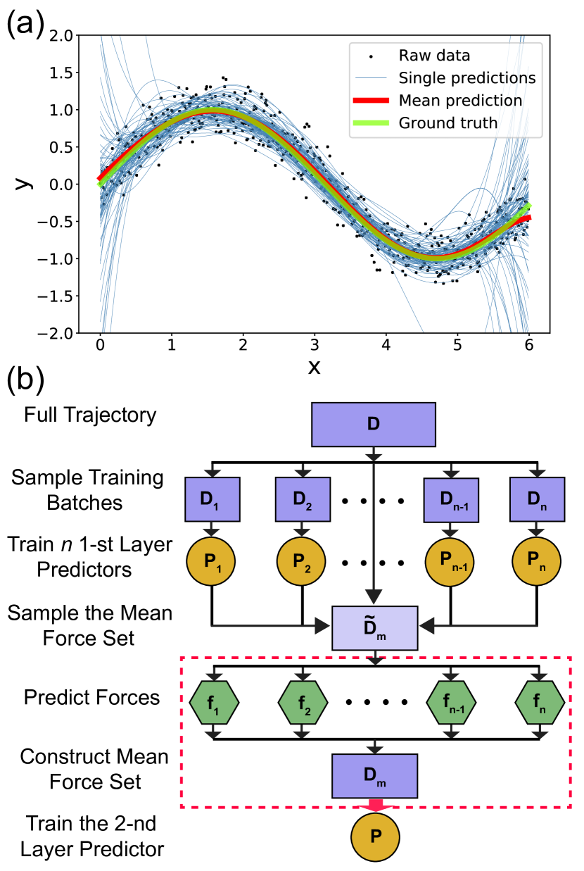
Figure 1: Schematic diagram illustrating the principle of ensemble learning. (a) 1 dimensional toy system. (b). 2-layer training scheme for learning CG force field using a GDML model.

Ensemble learning is a general and widely used machine learning trick to increase the predictive performance of a trained model by combining multiple sub-models (Opitz1999, ; Polikar, ; Rokach2010, ; Breiman1996, ; geman1992neural, ; Hansen1990, ; Schapire1990, ; Kuncheva2003, ; Bauer1999, ). In this work we use the idea at the basis of a particular ensemble learning method, called bootstrap-aggregation in the machine learning literature (Breiman1996, ), summarized in the following paragraphs and Algorithm 1. This method enables to train a GDML approach over millions of data points, a task that would be otherwise impossible.

In general, we generate a finite set of alternative GDML reconstructions from randomly drawn subsets of the full MD trajectory and average them to generate an estimate for the “expected” force prediction at each point. The variability in the individual training sets promotes flexibility in the structure across all models in the ensemble and enables us capture the variability in the dataset. We are then able to compute the expected value for each input by simply taking the mean of the ensemble.

Suppose we have a large data set $D:(x,y)$ for training that contains $N$ samples of pairs of points $x,y$. We would like to train a predictive model $f$ such that $y=f(x)$, using the data $D$. Instead of training a single model $f$ using the whole $N$ data points from $D,$ we first randomly sample $n$ batches: $\{D_{1},D_{2},...,D_{n}\},$ where each batch $D_{i}$ contains $N^{\prime}$ points. Usually $N$ is too large to efficiently train a single model, but it is possible to train sub-models on the different batches $\{f_{1},f_{2},...,f_{n}\}$ if $N^{\prime}<<N$. After training all the batches, the final predictive model $f$ is obtained as the average of all the sub-models:

$$f(x)=\frac{1}{n}\mathop{\sum_{i=1}^{n}f_{i}(x)}.$$ (12)

This enables us to generate consistent labels for a held-out subset of the trajectory, which then serves as the basis for another GDML reconstruction.

We demonstrate how bootstrapping aggregation is used on a simple example, where we learn an effective curve to fit a one dimensional data set. As shown in Fig. 1a, 600 raw points are uniformly sampled from $x\in[0,6]$, and the $y$ value of each point is assigned according to $y_{i}=\sin(x_{i})+0.2\xi$, where $\xi\sim N(0,1)$ is a random noise. These 600 points serve as the noisy training set. Instead of learning the curve using all 600 points at once, we bootstrap sample 100 batches from the full data set, where each batch contains only 20 points. We use a six-order polynomial function to fit 20 points in each batch, and the 100 fitted curves are shown in blue in Fig.1a. While each of these 100 blue curves oscillates around the mean and overfit the data, the mean of the 100 predictors (red curve) is smooth and agrees with the ground truth $y=\sin(x)$ (green curve) quite well.We use the idea of ensemble learning to apply GDML to CG problems, as a 2-layer procedure. Instead of training one single GDML model using all data, which usually exceed the upper memory limit of GDML, we train $N$ models $P_{i}|_{i=1}^{N}$ using $N$ data batches, where each batch contains only $n$ points. In this work, $N=n=1000$. Since 1000 points is far below the GDML limit, each GDML model $P_{i}$ is easy to train. After obtaining all $N$ GDML models $P_{i}|_{i=1}^{N}$, we use them to predict the forces $f_{i}$ corresponding to the $i$-th model for any given CG configuration $\mathbf{x}$ as $f_{i}=P_{i}(\mathbf{x})$. The mean force (CG force) for a configuration $\mathbf{x}$ is then the average of the forces for all the models: $f=\frac{1}{N}\sum_{i=1}^{N}f_{i}$ . This average force prediction could be directly used in the CG molecular simulation but the resulting model would be of low efficiency, since for each single configuration $\mathbf{x},$ the forces $f_{i}$ need to be evaluated for all $N$ models $P_{i}|_{i=1}^{N}$ to obtain an average CG force $f$.

This low evaluation efficiency motivates us to propose a 2-layer procedure to speed up the evaluation of the mean force prediction. We generate a new batch of data $\tilde{D}_{m}$ which contains $n^{\prime}$ points ($n^{\prime}=3000$ in this work). For all CG configurations in $\tilde{D}_{m}$, we use $N$ predictors to evaluate their forces and compute the mean forces. This produces a new data set $D_{m}$ where the $n^{\prime}$ configurations are associated to the corresponding mean forces. Constructing $D_{m}$ can be fast because the mean forces are computed only for $n^{\prime}$ points, usually a few thousands.

2Layer-GDML($D,N,n,n^{\prime}$)

1. Sample $N$ data batches from the original bulk data set $D:\{D_{1},D_{2},...,D_{N}\}$, each data batch $D_{i}$ contains $n$ randomly sampled points, each data point $d=(r,f)$ includes a molecular configuration part $r$ and a force part $f$

2. Sample one additional data batch $\tilde{D}_{m}$ from the original bulk data set $D$, that contains $n^{\prime}$ points, $d_{i}=(r_{i},f_{i})|_{i=1,2,...,n^{\prime}}$, each points $d_{i}$ also includes a molecular configuration part $r_{i}$ and a force part $f_{i}$, and $j$ indicates the point index in data batch $\tilde{D}_{m}$

3. For $i=1,...,N:$ # Loop over $N$ batches:

   1. Train GDML model $P_{i}$ using data batch $D_{i}$

   2. Predict forces for all $n^{\prime}$ configurations $r_{j}|_{j=1,2,...n^{\prime}}$ in data batch $\tilde{D}_{m}$ using model $P_{i}$, which is denoted as $f_{j}^{i}|_{j=1,2,...,n^{\prime}}$

4. Construct the mean force set $D_{m}$, which also includes $n^{\prime}$ points, the configuration part $r_{j}$ for each point is the same as $\tilde{D}_{m}$, but the force part $f_{j}$ is the averaged force computed using the $N$ GDML models: $f_{j}=\frac{1}{N}\sum_{i=1}^{N}f_{j}^{i}$

5. Train the 2nd-layer model $P$ using the constructed mean force set $D_{m}$

Algorithm 1 2-layer training scheme

Once the mean force set $D_{m}$ is obtained, we can train a single final model $P$ using the entire $D_{m}$. Since $D_{m}$ contains the mean forces, the final model $P$ also predicts the mean forces for the CG configurations. $P$ is easy to train due to small size of $D_{m}$ ($n^{\prime}$ is far below the GDML limit) and the force evaluation for the final model $P$ is much more efficient than by evaluating $N$ models $P_{i}|_{i=1}^{N}$. The general procedure of the 2-layer scheme is illustrated in Algorithm 1.

The hyperparameters that control the performance of the final model are the two kernel sizes $\sigma_{1},\sigma_{2}$, for each layer (see Eq. 11). Another hyperparameter is the regularization coefficient of the ridge term, and is set to the standard value ($\lambda=1\times 10^{-15}$) as in the original GDML paper (ChmielaEtAl_SciAdv17_EnergyConserving, ). We conduct a 2D cross-validation search to determine $\sigma_{1}$ and $\sigma_{2}$. The algorithm for the cross-validation of the ensemble learning GDML is shown in Algorithm 2. The parameters $N,n,n^{\prime},K$ are selected as $N=n=1000,n^{\prime}=3000,K=5,$ $K$ is the number of folds for the cross-validation, and the total number of points in $D$ is $1,000,000$.

2Layer-GDML-CV($D,N,n,n^{\prime},K$)

1. Sample $N$ data batches from the original bulk data set $D:\{D_{1},D_{2},...,D_{N}\}$, each data batch $D_{i}$ contains $n$ randomly sampled points, each points $d=(r,f)$ includes the molecular configuration part $r$ and the force part $f$

2. Sample one additional data batch $\tilde{D}_{m}$ from the original bulk data set $D$, that contains $n^{\prime}$ points, $d_{i}=(r_{i},f_{i})|_{i=1,2,...,n^{\prime}}$, each points $d_{i}$ also includes the molecular configuration part $r_{i}$ and the force part $f_{i}$, and $j$ indicates the point index in data batch $\tilde{D}_{m}$

3. For $i=1,...,N:$ # Loop over $N$ batches:

   1. Train GDML model $P_{i}$ using data batch $D_{i}$

   2. Predict forces for all $n^{\prime}$ configurations $r_{j}|_{j=1,2,...n^{\prime}}$ in data batch $\tilde{D}_{m}$ using model $P_{i}$, which is denoted as $f_{j}^{i}|_{j=1,2,...,n^{\prime}}$

4. Divide $N$ data batches into $K$ subsets of batches: $SD=\{SD_{1},SD_{2},...,SD_{K}\}$, where each subset $SD_{i}$ contains $N/K$ batches.

5. For the $j^{th}$ point in $\tilde{D}_{m}$, divide $N$ of its predicted forces $f_{j}^{i}|_{i=1,...,N}$ into subsets $SF_{j}=\{SF_{j,1},SF_{j,2},...,SF_{j,K}\}$, where each subset contains $N/K$ force tags that are consistent with the division in step 4, and $j=1,2,...,n^{\prime}$

6. For $l=1,...,K:$ Loop over $K$ cross-validation folds:

   1. For the $j^{th}$ point in $\tilde{D}_{m}$, compute the mean forces using all forces from $SF_{j}\backslash SF_{j,l}$ (excluding $SF_{j,l})$, where $j=1,2,...,n^{\prime}$, after obtaining the mean forces for all $n^{\prime}$ configurations in $\tilde{D}_{m}$, construct the $l^{th}$ mean force set $D_{m,l}$

   2. Train the $l^{th}$ second layer model $P2_{l}$ using $D_{m,l}$

   3. Compute the validation error of model $P2_{l}$ using all data points from the excluded set $SD_{l}$, and denote the error as $E_{l}$

7. Return cross-validation score $\frac{1}{K}\sum_{k=1}^{K}E_{k}$

Algorithm 2 2-layer training scheme with cross-validation

II.5 Stratified Sampling

Another crucial factor that impacts the overall performance of our machine learning model is the distribution of the training data. As our training data are obtained from extensive MD simulations, they are distributed according to the Boltzmann distribution in the molecule configuration space. If a small batch of data is randomly sampled from the whole data set, the large majority of the data will reside in low free energy regions, while data in high free energy region, such as transition barriers, are underrepresented. Fig. 2a shows that, in the case of alanine dipeptide, most of the data in a small batch of randomly selected points are located in the free energy minima on the left side of the $(\phi,\psi)$ dihedral angle space. If batches from this biased distribution are used in the ensemble learning, the errors for predicting the PMF in high free energy regions would be very large, because the models will not be trained efficiently in these sparse data regions.

In order to solve this issue, we sample the data for the batches uniformly in the $(\phi,\psi)$ dihedral angles space of alanine dipeptide, as shown in Fig. 2b. In this way, all relevant regions in the configurational space are equally represented in the training set, including transition states. The advantage of this strategic sampling is illustrated in more details in section III.

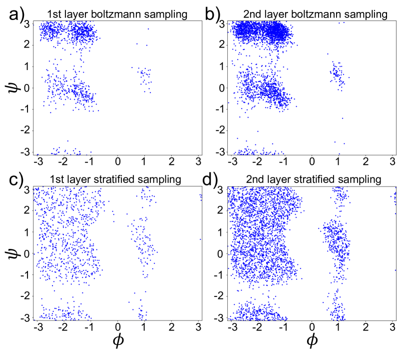
Figure 2: Stratified sampling of the training set for alanine-dipeptide in the dihedral angles $(\psi,\phi)$ space. (a) Regular (Boltzmann distributed) sampling of 1000 points for the 1st-layer. (b) Regular sampling of 3000 points for the 2nd-layer. (c) Uniformly stratified sampling of 1000 points in the $(\psi,\phi)$ space for the 1^st layer. (d) Uniformly stratified sampling of 3000 points in the $(\psi,\phi)$ space for the 2^nd layer.

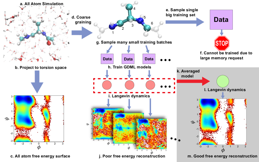
Figure 3: Pipeline of learning the CG forcefield with the GDML model. (a) All atom simulation of alanine dipeptide in water. (b) We compute the two dihedral angles $\phi$ and $\psi$, project the simulation data on to the $(\phi,\psi)$ space. (c) All-atom free energy surface in $(\phi,\psi)$ space. (d) The coarse graining model contains only six heavy atoms from the original molecule. (e) We could sample enough point for training a CG model, the data set is usually big. (f) Training the GDML model with one big data set requires large memory, which hinder the application of GDML to coarse graining a molecule. (g) Instead of sampling one big training set, we sample many smaller training sets. (h) We train GDML models with each small training set. (i) We use Langevin dynamics to simulate a CG MD trajectory with each trained GDML model. (j) Similar to (b) and (c), we compute the free enenrgy surface in $(\phi,\psi)$ space for each trajectory, and we find that these single models poorly recovered the correct free energy surface. (k) We can obtain an extra model which is the average of all models we trained in step (h). The averaging proceedure indicated by the red dashed box and arrow corresponds to the red box and arrow in Figure. 1(b). (l) We can simulate the averaged model using Lagevin dynamics. (m) The average CG model can correctly reconstruct the free energy surface of the molecule. The final result is highlighted in a light gray box.

II.6 Simulating the CG-GDML Model

After training the 2-layer GDML model, we use an over-damped Langevin dynamics to generate a trajectory and sample the CG potential $U(\mathbf{x};\theta)$:

$$\mathbf{x}_{t+\tau}=\mathbf{x}_{t}-\tau\frac{D}{k_{B}T}\nabla U(\mathbf{x}_{t})+\sqrt{2\tau D}\boldsymbol{\xi}$$ (13)

where $\mathbf{x}_{t}$ ($\mathbf{x}_{t+\tau}$) is the CG configuration at time $t$ ($t+\tau$), $\tau$ is the time step, $D$ is the diffusion constant, and $\xi$ is a vector of independent Gaussian random variables with zero-mean and identity covariance matrix (Wiener process). To sample the trained potential more efficiently, we generate 100 independent trajectories in parallel, with initial configurations randomly sampled from the original data set.

II.7 Including Physical Constraints

When an over-damped Langevin dynamics (Eq. 13) is used to generate a trajectory with a CG potential trained on a finite dataset, one undesired situation may happen: since the dynamics is stochastic, there is a chance that the simulated CG trajectory may diffuse away from the domain of the data used in the training, generating unphysical configurations. For example, the stretching of a bond too far away from the equilibrium distance is associated with a very high energy cost and is never observed in simulation with a force field at finite temperature. In simulation with a machine-learned CG potential, there is no mechanism for preventing such as unphysical bond-stretching. Similarly to what we proposed in our recent work (wang2019, ), this problem can be solved by including a prior potential energy $U_{prior}(\mathbf{x})$ incorporating physical prior knowledge on the system:

$$U(\mathbf{x};\boldsymbol{\theta})=U_{diff}(\mathbf{x;\boldsymbol{\theta}})+U_{\mathrm{prior}}(\mathbf{x})$$

where $U_{prior}(\mathbf{x})$ has harmonic terms modeling bond and angle stretching, with parameters extracted from the training data by Boltzmann inversion. $U_{diff}(\mathbf{x};\boldsymbol{\theta})$ is the difference between the total CG potential and $U_{prior}(\mathbf{x})$. The forces obey a similar relation:

$$\begin{array}[]{cc}-\nabla U(\mathbf{x};\boldsymbol{\theta})=-\nabla U_{diff}(\mathbf{x;\boldsymbol{\theta}})-\nabla U_{\mathrm{prior}}(\mathbf{x})\end{array}$$

so the loss function of the model becomes:

$$\chi^{2}(\boldsymbol{\theta})=\Bigl{\langle}\Bigl{\|}\xi(\mathbf{F}(\mathbf{r}))-\nabla U_{prior}(\mathbf{x})+\\ +\nabla U_{diff}(\xi(\mathbf{r});\boldsymbol{\theta})\Bigr{\|}^{2}\Bigr{\rangle}_{r}.$$ (14)

Differently from what was done in a neural network model (wang2019, ), the prior potential is not added directly to the trained model: the prior forces are first evaluated and subtracted from the all-atom forces, and the GDML is trained over this force difference. Once the model is trained, the total energy (and forces) is obtained by adding back the prior energy (and forces) to the one obtained from the trained model.

III Results

We illustrate the results of the approach discussed above on a simple molecular system, namely the coarse-graining of the alanine-dipeptide molecule from the atomistic model in explicit water into a 6-bead CG model. The all-atom model of alanine dipeptide consists of 22 atoms and 651 water molecules, for a total of a few thousand degrees of freedom. As illustrated in Fig. 3, for the CG representation we select the 5 central backbone atoms of the molecule, with additionally a 6^th atom to break the symmetry and differentiate right- or left- handed representations. The overall pipeline for the coarse graining and the training procedure that is discussed below is also summarized in Figure 3.

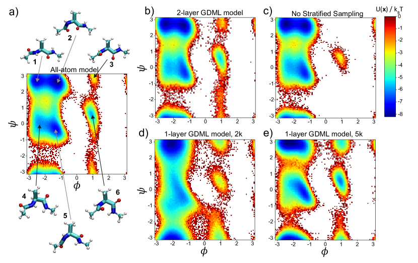
Figure 4: Free energy surface in $(\psi,\phi)$ space for the trained GDML models. (a) reference (all-atom) free energy landscape, and all representative configurations of the molecule in the six minima sampled from the all-atom trajectory (CPK representation) and from a CG simulation with the 2-layer GDML model (thick bonds). (b) Free energy landscape from the 2-layer GDML model. (c) Free energy from a 2-layer GDML model with no stratified sampling. (d) Free energy from a traditional single-layer GDML model, trained with 2000 points. (e) Free energy from a traditional single-layer GDML model, trained with 5000 points.

We compute the free energy of the alanine dipeptide as a function of the two dihedral angles $\phi,\psi$, where $\phi$ is defined by atoms 1, 2, 3, 5, and $\psi$ by atoms 2, 3, 5, 6 (see Fig. 3). As shown in Fig. 4a, there are six metastable states in the free energy landscape of the all-atom model of alanine dipeptide. Fig.4b shows that the final 2-layer GDML CG model correctly reproduces the free energy landscape of alanine dipeptide: the free energy obtained from the trajectories (generated by numerical integration of Eq.13) of the CG model also exhibits six minima, with depths close to the ones of the corresponding minima in the all-atom model. Representative configurations from the six metastable states are shown in Fig.4a for the all-atom (CPK representation) and the CG model (thick bond representation). Moreover, as shown in SI Fig. LABEL:fig:angle_bond_distribution-1, the bond and angle distribution from the CG simulation are also consistent with the all atom simulation.

The GDML model shown in 4b is optimized based on the minimum cross-validation error over a 2-dimensional grid, spanned by the parameters $\sigma_{1}$ and $\sigma_{2}$, which are the kernel width for the 1^st and the 2^nd layer models. We find that the values $(\sigma_{1},\sigma_{2})=(100,10)$ give the smallest cross-validation error. Details on the cross-validation search can be found in SI Fig. LABEL:fig:Cross_validation-1.

Fig. 4c reports the free energy landscape corresponding to a CG model obtained with a 2-layer GDML but where the selection of the data for the sub-model is performed according to the Boltzmann distribution (that is, uniform sampling along the MD trajectory) instead of the stratified sampling scheme discussed above (uniform sampling in the $\phi,\psi$ space). While the free energy around the region of the deepest free energy minima in the $\phi,\psi$ space is quite accurate, the lowly populated metastable state (indicated as state 3 in 4a) is completely missing in 4c, because of the scarcity of training points in this region.

As a comparison, Fig. 4d shows the results when a single-layer GDML model is trained on only 2000 points. Although this model identifies the general location of the metastable states, the free energy landscape is significantly distorted with respect to the all-atom one. This poor reconstruction performance is due to the limited size of the training set, which is not extensive enough to enable a stable estimate of the expected forces for the reduced representation of the input. We also trained a single-layer GDML model on 5000 points. As shown in Fig. 4 e, the free energy of this model presents a slightly improvement with respect Fig. 4d because of the increased number of training points. However, the overall quality is still low comparing to the atomistic model. We expect the reconstructed free energy to improve further if we trained a model using much more data, but this is hindered by the memory requirement: it requires about 160 GB memory to train a model with 5000 points, which is almost at the upper limit of our computational ability.

To quantify the performance of the different approaches, we compute the mean square error (MSE) of the free energy difference of the different CG models compared to the atomistic model (Fig. 4a, Table 1, see (wang2019, ) for details). As expected, the 2-layer GDML model has the smallest free energy MSE, which is about $0.363\pm 0.112\,(k_{B}T)^{2}$, when it is trained with all 1000 batches. The single layer GDML gives the largest free energy difference ( $2.947\,(k_{B}T)^{2}$ if trained with 2000 points, and $1.641\,(k_{B}T)^{2}$ if trained with 5000 points). If no stratified sampling is used, the free energy difference is $0.861\,(k_{B}T)^{2}$, and most of this value is due to the discrepancies in the free energy $\phi>0$ region.

As a baseline, we also compute the free energy difference obtained by a CG model designed by means of a neural network, CGnet (wang2019, ). Previously, we have applied CGnet to alanine-dipeptide, but it was a model based on a 5 atom CG scheme, and we included two dihedral angles as input features to break the symmetry. To make the CGnet model consistent with the CG scheme used in this work, we modified it to contain 6 atoms (as in the GDML model), and no dihedral angles features were included (only distances are used as input). This CGnet model is trained with the same number of points as the GDML model (i.e. 1,000,000 points from 1000 batches). The resulting CGnet free energy MSE is $0.475\pm 0.103\,(k_{B}T)^{2}$, a value slightly larger than the 2-layer GDML model. This result shows that the accuracy of a kernel approach can indeed be comparable to or even better than a neural network approach on the same system.

We have also investigated the effect of the batch number (or the training set size). We computed the cross-validation error with different training set size, from $10$ to $1000$ batches for the GDML model, or equivalentely from $10,000$ to $1,000,000$ points for CGnet. Fig. 5a shows that as the batch number increases from $10$ to $1000$, the cross-validation error for GDML model drops quickly, and reaches convergence with a batch number $>600$ . The cross-validation error for CGnet is significantly larger than for the GDML model when the number of batches (or, equivalently, the training set size) is small. When the batch number is larger than 200, the cross-validation error for CGnet becomes smaller than for GDML. Similarly, if we compare the free energy MSEs, as shown in Fig. 5b, the free energy constructed by GDML with a small training set is significantly better than the corresponding free energy constructed by CGnet. On the other hand, with a large training set, the MSEs are comparable to each other. Typical free energy profiles are shown in Fig. 6a-d, and their corresponding MSE values are shown Table 1. These results show that with enough data, the 2-layer GDML model and CGnet perform similarly well. However, the 2-layer GDML model is more data efficient and has a better ability to extrapolate the force prediction to unsampled configurations, thus outperforming CGnet for small training sets.

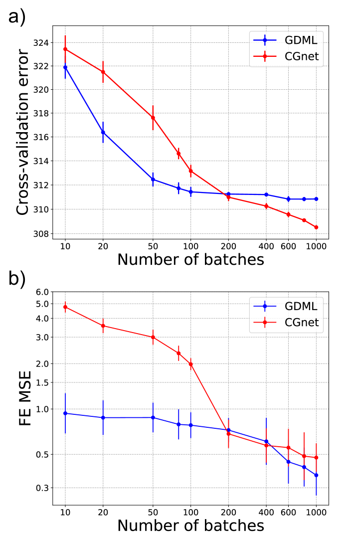
Figure 5: Cross-validation error (a) and free energy mean square error (MSE) (b) as a function of the number of batches. For CGnet, the training set size is equal to $1000\times$ number of batches. The units for the crosss-validation error are $kcal/mol^{2}/\text{\AA}^{2}$, while the units for the free energy MSE are $(k_{B}T)^{2}$.

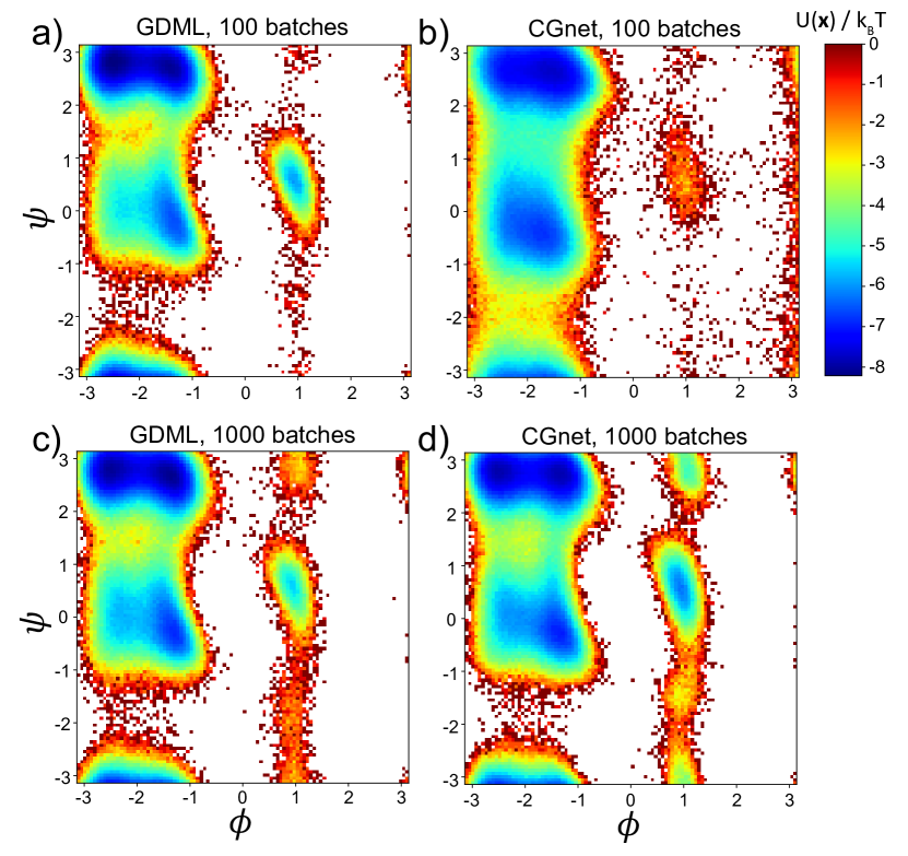
Figure 6: Free energy as a function of the alanine dipeptide dihedral angles, for a 2-layer GDML CG model with number of batches $N_{Batch}=100$ (a) and $N_{Batch}=1000$ (c), and for CGnet with $N_{Batch}=100$ (b) and $N_{Batch}=1000$ (d).

Table 1: Free energy mean square error (MSE) comparison for different CG models trained with different number of points, which is in the unit of thousand (k). The error is computed as the mean square error of the free energy of alanine-dipeptide in ($\psi,\phi$) space, relative to the atomistic free energy (wang2019, ). The MSE values are in units of $(k_{B}T)^{2}$.

Model	100 k	1000 k	2 k	5 k
CGnet	$1.982\pm 0.181$	$0.475\pm 0.103$	-	-
2-layer GDML	$0.781\pm 0.154$	$0.363\pm 0.112$	-	-
Boltz. Samp. 2-layer GDML	-	$0.861\pm 0.167$	-	-
1-layer GDML	-	-	$2.947\pm 0.264$	$1.641\pm 0.243$

IV Conclusions

In this work we combine the idea of ensemble learning with GDML, to apply it to the coarse graining problem. GDML is a kernel method to learn molecular force fields from data, and allows to model nonlinearity and multi-body effects without the need of providing a functional form for the potential. The GMDL approach was originally proposed to learn molecular forces from quantum simulation data. When quantum calculations are used, the error on the force matching loss could in in principle be zero, and a few thousand points are enough to construct and build an accurate, smooth and conserved force field. However, when applied to coarse-graining , the force matching loss contains a non zero term due to the dimensionality reduction and the learning problem becomes very noisy. For this reason a lot more data points are needed from atomistic simulations to learn a CG potential of mean force. The large amount of input data would presently hinder the application of GDML to the CG problem. In order to circumvent this problem, we use ensemble learning. The basic idea consists in breaking down the learning problem into small batches, that can be more easily solved, and combine the resulting different models into a final solution. Following this approach, we do not train one single GDML model using all the data, but propose a 2-layer training scheme: in the first layer, we generate $N$ data batches, each containing a number of points far below the GDML limit. $N$ models are trained on the different batches and are combined into a final model by taking the average. We show that the prediction of the CG 2-layer model accurately reproduces the thermodynamics of the atomistic model.

Consistently with previous work (wang2019, ), we show that, when applying machine learning methods to design force fields for molecular systems, the addition of physical constraints enforce proper asymptotic of the model. In the design of CG potentials, physical constraints can be introduced by means of a prior potential energy term that prevent the appearance of spurious effects in non-physical regions of the configurational landscape.

A good GDML model should be able to construct a smooth and globally connected conserved force field. However, when the 2-layer approach is used some of the molecular configurations with high free energy are poorly sampled in the training set, introducing large errors in the resulting model. In order to solve this problem, we sample the data uniformly in the low dimensional space defined by two collective coordinates rather than uniformly from the simulation time series. In the example of alanine dipeptide discussed here, the dihedral angles $\phi,\psi$ are chosen as collective coordinates.

In our previous work, we proposed CGnet (wang2019, ), a neural network approach to design CG models. The overall free energy reconstruction obtained with the GDML model is comparably accurate as what was obtained with CGnet when the training set size is sufficiently large. However, the GDML model is significantely more accurate when the training set size is small, indicating that a kernel approach is data-efficient and could in principle provide more accurate CG models especially with small training sets.

However, there are still several challenges in order to apply GDML for the coarse-graining of macromolecular systems. In larger systems, a more general definition is needed for the collective coordinates defining the low dimensional space for the uniform sampling of the training batches. These collective coordinates could in principle be extracted from the trajectory data (RohrdanzEtAl_AnnRevPhysChem13_MountainPasses, ; NoeClementi_COSB17_SlowCVs, ), for instance by means of time-lagged Independent Component Analysis (tICA)(Perez-Hernandez2013, ; SchwantesPande_JCTC13_TICA, ; ZieheMueller_ICANN98_TDSEP, ; Belouchrani1997, ; Molgedey_94, ), kernel PCA(Klaus1997, ; Klaus1998, ; Klaus2001, ) or diffusion maps (RohrdanzClementi_JCP134_DiffMaps, ).

The decomposition of the large input data set into an ensemble of small batches has been used here to solve memory issues when training a GDML model. However, the computation is still expensive and we expect it to become even more expensive as the size of the molecular system increases. As the number of data batches and batch size grow, the Nyström approximation of the kernel or other numerical approaches may be a promising solution to increase the computational efficiency.

As for the neural network model, the GDML model trained by force matching can capture the thermodynamics of the system, but there is no guarantee that the dynamics is also preserved. Alternative approaches need to be defined to solve this problem (Nuske2019, ).

Finally, the GDML model presented here is trained on a specific molecule, and it is not directly transferable to different systems. Ultimately, a transferable CG model would be needed for the general application to large systems that can not be simulated by atomistic simulations. The trade-off between accuracy and transferability in CG models is an open research question that we will investigate in future work.

V Supplementary Material

See Supplementary Material for more details about the hyperparameter search, a discussion on the prior energy, and more information on the descriptors used in the GDML.

The data that support the findings of this study are available from the corresponding author upon reasonable request.

References

- [1] K. Lindorff-Larsen, S. Piana, R. O. Dror, and D. E. Shaw. How fast-folding proteins fold. Science, 334:517–520, 2011.
- [2] I. Buch, M. J. Harvey, T. Giorgino, D. P. Anderson, and G. De Fabritiis. High-throughput all-atom molecular dynamics simulations using distributed computing. J. Chem. Inf. Model., 50:397–403, 2010.
- [3] M. Shirts and V. S. Pande. Screen savers of the world unite! Science, 290:1903–1904, 2000.
- [4] R. O. Dror, A. C. Pan, D. H. Arlow, D. W. Borhani, P. Maragakis, Y. Shan, H. Xu, and D. E. Shaw. Pathway and mechanism of drug binding to g-protein-coupled receptors. Proc. Natl. Acad. Sci. USA, 108:13118–13123, 2011.
- [5] D. Shukla, Y. Meng, B. Roux, and V. S. Pande. Activation pathway of src kinase reveals intermediate states as targets for drug design. Nat. Commun., 5:3397, 2014.
- [6] N. Plattner and F. Noé. Protein conformational plasticity and complex ligand binding kinetics explored by atomistic simulations and markov models. Nat. Commun., 6:7653, 2015.
- [7] N. Plattner, S. Doerr, G. D. Fabritiis, and F. Noé. Protein-protein association and binding mechanism resolved in atomic detail. Nat. Chem., 9:1005–1011, 2017.
- [8] F. Paul, C. Wehmeyer, E. T. Abualrous, H. Wu, M. D. Crabtree, J. Schöneberg, J. Clarke, C. Freund, T. R. Weikl, and F. Noé. Protein-ligand kinetics on the seconds timescale from atomistic simulations. Nat. Commun., 8:1095, 2017.
- [9] F. Noé, A. Tkatchenko, K.-R. Müller, and C. Clementi. Machine learning for molecular simulation. Ann. Rev. Phys. Chem., in press, 2020.
- [10] D. Frenkel and B. Smit. Understanding Molecular Simulation: From Algorithms to Applications. Academic Press, 2 edition, 2001.
- [11] G. M. Torrie and J. P. Valleau. Nonphysical sampling distributions in monte carlo free-energy estimation: Umbrella sampling. J. Comput. Phys., 23(2):187–199, 1977.
- [12] J. Kästner. Umbrella sampling. Wiley Interdisciplinary Reviews: Computational Molecular Science, 1(6):932–942, 2011.
- [13] R. H. Swendsen and J.-S. Wang. Replica monte carlo simulation of spin-glasses. Phys. Rev. Lett., 57:2607–2609, Nov 1986.
- [14] R. M. Neal. Sampling from multimodal distributions using tempered transitions. Stat. Comput., 6(4):353–366, Dec 1996.
- [15] R. Rajamani, K. J. Naidoo, and J. Gao. Implementation of an adaptive umbrella sampling method for the calculation of multidimensional potential of mean force of chemical reactions in solution. Proteins, 24:1775–1781, 2003.
- [16] J. Preto and C. Clementi. Fast recovery of free energy landscapes via diffusion-map-directed molecular dynamics. Phys. Chem. Chem. Phys., 16:19181–19191, 2014.
- [17] G. R. Bowman, D. L. Ensign, and V. S. Pande. Enhanced Modeling via Network Theory: Adaptive Sampling of Markov State Models. J. Chem. Theory Comput., 6(3):787–794, 2010.
- [18] C. Clementi. Coarse-grained models of protein folding: Toy-models or predictive tools? Curr. Opin. Struct. Biol., 18:10–15, 2008.
- [19] A. Davtyan, N. P. Schafer, W. Zheng, C. Clementi, P. G. Wolynes, and G. A. Papoian. AWSEM-MD: Protein structure prediction using coarse-grained physical potentials and bioinformatically based local structure biasing. J. Phys. Chem. B, 116(29):8494–8503, 2012.
- [20] S. Izvekov and G. A. Voth. A multiscale coarse-graining method for biomolecular systems. J. Phys. Chem. B, 109(7):2469–2473, 2005.
- [21] S. J. Marrink, A. H. de Vries, and A. E. Mark. Coarse grained model for semiquantitative lipid simulations. J. Phys. Chem. B, 108(2):750–760, 2004.
- [22] F. Müller-Plathe. Coarse-graining in polymer simulation: From the atomistic to the mesoscopic scale and back. ChemPhysChem, 3(9):754–769, sep 2002.
- [23] W. G. Noid. Perspective: Coarse-grained models for biomolecular systems. J. Chem. Phys., 139(9):090901, 2013.
- [24] S. O. Nielsen, C. F. Lopez, G. Srinivas, and M. L. Klein. A coarse grain model for n-alkanes parameterized from surface tension data. J. Chem. Phys., 119(14):7043–7049, 2003.
- [25] S. Matysiak and C. Clementi. Optimal combination of theory and experiment for the characterization of the protein folding landscape of s6: How far can a minimalist model go? J. Mol. Biol., 343:235–248, 2004.
- [26] S. Matysiak and C. Clementi. Minimalist protein model as a diagnostic tool for misfolding and aggregation. J. Mol. Biol., 363:297–308, 2006.
- [27] J. Chen, J. Chen, G. Pinamonti, and C. Clementi. Learning effective molecular models from experimental observables. J. Chem. Theory Comput., 14(7):3849–3858, 2018.
- [28] A. P. Lyubartsev and A. Laaksonen. Calculation of effective interaction potentials from radial distribution functions: A reverse monte carlo approach. Phys. Rev. E, 52(4):3730–3737, 1995.
- [29] M. Praprotnik, L. D. Site, and K. Kremer. Multiscale simulation of soft matter: From scale bridging to adaptive resolution. Ann. Rev. Phys. Chem., 59(1):545–571, 2008.
- [30] Y. Wang, W. G. Noid, P. Liu, and G. A. Voth. Effective force coarse-graining. Phys. Chem. Chem. Phys., 11(12):2002, 2009.
- [31] M. S. Shell. The relative entropy is fundamental to multiscale and inverse thermodynamic problems. J. Phys. Chem., 129(14):144108, 2008.
- [32] F. Noé, S. Olsson, J. Köhler, and H. Wu. Boltzmann generators: Sampling equilibrium states of many-body systems with deep learning. Science, 365(6457), 2019.
- [33] F. Noé, G. D. Fabritiis, and C. Clementi. Machine learning for protein folding and dynamics. Curr. Op. Struct. Biol., 60:77 – 84, 2020.
- [34] K. T. Schütt, M. Gastegger, A. Tkatchenko, K.-R. Müller, and R. J. Maurer. Unifying machine learning and quantum chemistry with a deep neural network for molecular wavefunctions. Nat. Commun., 10(1):5024, 2019.
- [35] J. Behler and M. Parrinello. Generalized neural-network representation of high-dimensional potential-energy surfaces. Phys. Rev. Lett., 98:146401, 2007.
- [36] A. P. Bartók, M. C. Payne, R. Kondor, and G. Csányi. Gaussian approximation potentials: The accuracy of quantum mechanics, without the electrons. Phys. Rev. Lett., 104(13), 2010.
- [37] M. Rupp, A. Tkatchenko, K.-R. Müller, and O. A. von Lilienfeld. Fast and accurate modeling of molecular atomization energies with machine learning. Phys. Rev. Lett., 108(5), 2012.
- [38] A. P. Bartók, M. J. Gillan, F. R. Manby, and G. Csányi. Machine-learning approach for one- and two-body corrections to density functional theory: Applications to molecular and condensed water. Phys. Rev. B, 88(5), 2013.
- [39] J. S. Smith, O. Isayev, and A. E. Roitberg. ANI-1: an extensible neural network potential with DFT accuracy at force field computational cost. Chem. Sci., 8(4):3192–3203, 2017.
- [40] A. P. Bartók, S. De, C. Poelking, N. Bernstein, J. R. Kermode, G. Csányi, and M. Ceriotti. Machine learning unifies the modeling of materials and molecules. Sci. Adv., 3(12), 2017.
- [41] K. T. Schütt, F. Arbabzadah, S. Chmiela, K. R. Müller, and A. Tkatchenko. Quantum-chemical insights from deep tensor neural networks. Nat. Commun., 8:13890, 2017.
- [42] J. S. Smith, B. Nebgen, N. Lubbers, O. Isayev, and A. E. Roitberg. Less is more: Sampling chemical space with active learning. J. Chem. Phys., 148(24):241733, 2018.
- [43] K. T. Schütt, H. E. Sauceda, P.-J. Kindermans, A. Tkatchenko, and K.-R. Müller. SchNet - a deep learning architecture for molecules and materials. J. Chem. Phys., 148(24):241722, 2018.
- [44] A. Grisafi, D. M. Wilkins, G. Csányi, and M. Ceriotti. Symmetry-adapted machine learning for tensorial properties of atomistic systems. Phys. Rev. Lett., 120(3), 2018.
- [45] G. Imbalzano, A. Anelli, D. Giofré, S. Klees, J. Behler, and M. Ceriotti. Automatic selection of atomic fingerprints and reference configurations for machine-learning potentials. J. Chem. Phys., 148(24):241730, 2018.
- [46] T. T. Nguyen, E. Székely, G. Imbalzano, J. Behler, G. Csányi, M. Ceriotti, A. W. Götz, and F. Paesani. Comparison of permutationally invariant polynomials, neural networks, and gaussian approximation potentials in representing water interactions through many-body expansions. J. Chem. Phys., 148(24):241725, 2018.
- [47] L. Zhang, J. Han, H. Wang, W. A. Saidi, R. Car, and W. E. End-to-end symmetry preserving inter-atomic potential energy model for finite and extended systems. arXiv:1805.09003, 2018.
- [48] L. Zhang, J. Han, H. Wang, R. Car, and W. E. Deep potential molecular dynamics: a scalable model with the accuracy of quantum mechanics. Phys. Rev. Lett., 120:143001, 2018.
- [49] T. Bereau, R. A. DiStasio, A. Tkatchenko, and O. A. V. Lilienfeld. Non-covalent interactions across organic and biological subsets of chemical space: Physics-based potentials parametrized from machine learning. J. Chem. Phys., 148:241706, 2018.
- [50] S. Chmiela, A. Tkatchenko, H. E. Sauceda, I. Poltavsky, K. T. Schütt, and K.-R. Müller. Machine learning of accurate energy-conserving molecular force fields. Sci. Adv., 3:e1603015, 2017.
- [51] S. Chmiela, H. E. Sauceda, K.-R. Müller, and A. Tkatchenko. Towards exact molecular dynamics simulations with machine-learned force fields. Nature Commun., 9:3887, 2018.
- [52] A. Mardt, L. Pasquali, H. Wu, and F. Noé. Vampnets: Deep learning of molecular kinetics. Nat. Commun., 9:5, 2018.
- [53] H. Wu, A. Mardt, L. Pasquali, and F. Noé. Deep generative markov state models. In S. Bengio, H. Wallach, H. Larochelle, K. Grauman, N. Cesa-Bianchi, and R. Garnett, editors, Advances in Neural Information Processing Systems 31, pages 3975–3984. Curran Associates, Inc., 2018.
- [54] C. Wehmeyer and F. Noé. Time-lagged autoencoders: Deep learning of slow collective variables for molecular kinetics. J. Chem. Phys., 148:241703, 2018.
- [55] C. X. Hernández, H. K. Wayment-Steele, M. M. Sultan, B. E. Husic, and V. S. Pande. Variational encoding of complex dynamics. arXiv:1711.08576, 2017.
- [56] J. M. L. Ribeiro, P. Bravo, Y. Wang, and P. Tiwary. Reweighted autoencoded variational bayes for enhanced sampling (rave). J. Chem. Phys., 149:072301, 2018.
- [57] S. T. John and G. Csányi. Many-body coarse-grained interactions using gaussian approximation potentials. J. Phys. Chem. B, 121(48):10934–10949, 2017.
- [58] L. Zhang, J. Han, H. Wang, R. Car, and W. E. DeePCG: constructing coarse-grained models via deep neural networks. arXiv:1802.08549, 2018.
- [59] J. Wang, S. Olsson, C. Wehmeyer, A. Pérez, N. E. Charron, G. de Fabritiis, F. Noé, and C. Clementi. Machine learning of coarse-grained molecular dynamics force fields. ACS Cent. Sci., April 2019.
- [60] W. G. Noid, J.-W. Chu, G. S. Ayton, V. Krishna, S. Izvekov, G. A. Voth, A. Das, and H. C. Andersen. The multiscale coarse-graining method. I. A rigorous bridge between atomistic and coarse-grained models. J. Chem. Phys., 128(24):244114, 2008.
- [61] S. Chmiela, H. E. Sauceda, I. Poltavsky, K.-R. Müller, and A. Tkatchenko. sgdml: Constructing accurate and data efficient molecular force fields using machine learning. Comput. Phys. Commun., 240:38 – 45, 2019.
- [62] L. Boninsegna, R. Banisch, and C. Clementi. A data-driven perspective on the hierarchical assembly of molecular structures. J. Chem. Theory Comput., 14(1):453–460, 2018.
- [63] A. V. Sinitskiy, M. G. Saunders, and G. A. Voth. Optimal number of coarse-grained sites in different components of large biomolecular complexes. J. Phys. Chem. B, 116(29):8363–8374, 2012.
- [64] W. Wang and R. Gómez-Bombarelli. Coarse-graining auto-encoders for molecular dynamics. Npj Computat. Mater., 5(1), 2019.
- [65] V. N. Vapnik. An overview of statistical learning theory. IEEE Trans. Neur. Net., 10, 1999.
- [66] C. E. Rasmussen. Gaussian processes in machine learning. In Advanced lectures on machine learning, pages 63–71. Springer, 2004.
- [67] M. L. Stein. Interpolation of Spatial Data - Some Theory for Kriging. Springer-Verlag New York, 1999.
- [68] D. Opitz and R. Maclin. Popular ensemble methods: An empirical study. J. Artif. Intell. Res., 11:169–198, 1999.
- [69] R. Polikar. Ensemble based systems in decision making. IEEE Circuits Syst. Mag., 6(3):21–45, 2006.
- [70] L. Rokach. Ensemble-based classifiers. Artif. Intell. Rev., 33(1):1–39, Feb 2010.
- [71] L. Breiman. Bagging predictors. Mach. Learn., 24(2):123–140, 1996.
- [72] S. Geman, E. Bienenstock, and R. Doursat. Neural networks and the bias/variance dilemma. Neural Comput., 4(1):1–58, 1992.
- [73] L. K. Hansen and P. Salamon. Neural network ensembles. EEE Trans. Pattern Anal. Mach. Intell., 12(10):993–1001, Oct 1990.
- [74] R. E. Schapire. The strength of weak learnability. Mach. Learn., 5(2):197–227, Jun 1990.
- [75] L. I. Kuncheva and C. J. Whitaker. Measures of diversity in classifier ensembles and their relationship with the ensemble accuracy. Mach. Learn., 51(2):181–207, May 2003.
- [76] E. Bauer and R. Kohavi. An empirical comparison of voting classification algorithms: Bagging, boosting, and variants. Mach. Learn., 36(1):105–139, Jul 1999.
- [77] M. A. Rohrdanz, W. Zheng, and C. Clementi. Discovering mountain passes via torchlight: methods for the definition of reaction coordinates and pathways in complex macromolecular reactions. Ann. Rev. Phys. Chem., 64:295–316, 2013.
- [78] F. Noé and C. Clementi. Collective variables for the study of long-time kinetics from molecular trajectories: theory and methods. Curr. Opin. Struc. Biol., 43:141–147, 2017.
- [79] G. Pérez-Hernández, F. Paul, T. Giorgino, G. De Fabritiis, and F. Noé. Identification of slow molecular order parameters for Markov model construction. J. Chem. Phys., 139(1), 2013.
- [80] C. R. Schwantes and V. S. Pande. Improvements in markov state model construction reveal many non-native interactions in the folding of ntl9. J. Chem. Theory Comput., 9:2000–2009, 2013.
- [81] A. Ziehe and K.-R. Müller. TDSEP — an efficient algorithm for blind separation using time structure. In ICANN 98, pages 675–680. Springer Science and Business Media, 1998.
- [82] A. Belouchrani, K. Abed-Meraim, J. . Cardoso, and E. Moulines. A blind source separation technique using second-order statistics. IEEE Trans. Signal Process., 45(2):434–444, Feb 1997.
- [83] L. Molgedey and H. G. Schuster. Separation of a mixture of independent signals using time delayed correlations. Phys. Rev. Lett., 72:3634–3637, 1994.
- [84] B. Schölkopf, A. Smola, and K.-R. Müller. Kernel principal component analysis. In W. Gerstner, A. Germond, M. Hasler, and J.-D. Nicoud, editors, Artificial Neural Networks — ICANN’97, pages 583–588, Berlin, Heidelberg, 1997. Springer Berlin Heidelberg.
- [85] B. Schölkopf, A. Smola, and K.-R. Müller. Nonlinear component analysis as a kernel eigenvalue problem. Neural Comput., 10(5):1299–1319, 1998.
- [86] K. R. Muller, S. Mika, G. Ratsch, K. Tsuda, and B. Scholkopf. An introduction to kernel-based learning algorithms. IEEE Trans. Neural Netw., 12(2):181–201, March 2001.
- [87] M. A. Rohrdanz, W. Zheng, M. Maggioni, and C. Clementi. Determination of reaction coordinates via locally scaled diffusion map. J. Chem. Phys., 134:124116, 2011.
- [88] F. Nüske, L. Boninsegna, and C. Clementi. Coarse-graining molecular systems by spectral matching. J. Chem. Phys., 151(4):044116, 2019.