Asymptotic and exponential decay in mean square for delay geometric Brownian motion

Abstract.

We derive sufficient conditions for asymptotic and monotone exponential decay in mean square of solutions of the geometric Brownian motion with delay. The conditions are written in terms of the parameters and are explicit for the case of asymptotic decay. For exponential decay, they are easily resolvable numerically. The analytical method is based on construction of a Lyapunov functional (asymptotic decay) and forward-backward estimate for the square mean (exponential decay).

Keywords: Geometric Brownian Motion, delay, asymptotic decay, exponential decay.

2010 MR Subject Classification: 34K11, 34K25, 34K50, 60H10

1. Introduction and main result

Geometric Brownian motion (also called Ornstein-Uhlenbeck process with multiplicative noise) is the strong solution of the Itô stochastic differential equation

(1.1) $$\mathrm{d}w(t)=-\lambda w(t)\mathrm{d}t+\sigma w(t)\mathrm{d}B_{t},$$

where $\lambda$ and $\sigma$ are real parameters and $\mathrm{d}B_{t}$ denotes the one-dimensional Wiener process. It is one of the stochastic processes very often used in applications, in particular in financial mathematics to model stock prices in the Black-Scholes model [8]. However, modelling the price process by geometric Brownian motion has been criticized because the past of the volatility is not taken into account. Consequently, [1] suggests to replace the multiplicative constants $\lambda$ and $\sigma$ in (1.1) by some linear functionals on the space of continuous functions. Here we make the generic choice of constant delay model, i.e., we evaluate $w$ in the right-hand side of (1.1) at the past time instant $t-\tau$, with $\tau>0$. This leads to the following delay Itô stochastic differential equation

(1.2) $$\mathrm{d}w(t)=-\lambda w(t-\tau)\mathrm{d}t+\sigma w(t-\tau)\mathrm{d}B_{t}.$$

The main goal of this paper is to derive sufficient conditions for asymptotic and monotone (exponential) decay in mean square of the solutions of (1.2).

Solutions of delay (retarded) differential equations are well known to develop oscillations in certain regimes [15]. Taking the expectation of (1.2), we obtain the deterministic delay differential equation for $u(t):=\mathbb{E}[w(t)]$,

(1.3) $$\dot{u}(t)=-\lambda u(t-\tau).$$

Despite its simplicity, it exhibits a surprisingly rich qualitative dynamics. An analysis of the corresponding characteristic equation

$$z+\lambda\tau e^{-z}=0,$$

where $z\in\mathbb{C}$, reveals that:

• If $0<\lambda\tau<e^{-1}$, then $u=0$ is asymptotically stable. Solutions of (1.3) subject to constant nonzero initial datum on $[-\tau,0]$ tend to zero monotonically (exponentially) as $t\to\infty$.

• If $e^{-1}<\lambda\tau<\pi/2$, then $u=0$ is asymptotically stable, but every nontrivial solution of (1.3) is oscillatory, i.e., changes sign infinitely many times on $(0,\infty)$.

• If $\lambda\tau>\pi/2$, then $u=0$ is unstable.

We refer to Chapter 2 of [15] and [7] for details. Consequently, two very natural questions arise in connection with (linear) delay differential equations: Under which conditions does the solution tend to zero asymptotically as $t\to\infty$, and under which conditions is this decay monotone? This paper is devoted to the study of these two questions in mean square sense for solutions of (1.2).

Various types of sufficient conditions for stability (in some sense) of equation (1.2) and its generalizations have been established in the literature, see [10, 12, 13] for an overview. However, to our best knowledge, none of them provide an explicit formula relating the parameters $\lambda$, $\tau$ and $\sigma$. A remarkable result by [1] states that

$$\lim_{t\to\infty}\mathbb{E}\left[|w(t)|^{2}\right]=0\qquad\qquad\mbox{if and only if}\qquad\qquad\int_{0}^{\infty}r_{\lambda}(t)^{2}\mathrm{d}t<\frac{1}{\sigma^{2}},$$

where $w$ is a solution of (1.2) and $r_{\lambda}$ is the fundamental solution of the delayed ODE (1.3), i.e., formally, $r_{\lambda}$ solves (1.3) subject to the initial condition $u(t)=\chi_{\{0\}}(t)$ for $t\in(-\tau,0]$. The fundamental solution $r_{\lambda}$ can be constructed by the method of steps [15], however, to out best knowledge, analytic evaluation of its $L^{2}(0,\infty)$-norm is an open problem. An explicit sufficient condition for asymptotic mean square stability of (1.2) has been provided in [4], together with numerical experiments (systematic Monte Carlo simulations) giving a hint about how far the analytical result is from optimal. However, [4] considers (1.2) only as a special case of a more general delay stochastic system, which leads to some inefficiencies. Our first result, Theorem 1, improves the sufficient condition of [4], and is still explicit in terms of the parameter values. The proof is based on a construction of an appropriate Lyapunov functional. Our second result, Theorem 2, is based on a forward-backward estimate for the mean square and provides sufficient condition for exponential decay in mean square of solutions of (1.2). The condition, written in terms of $\lambda$, $\tau$ and $\sigma$, is not fully explicit, however, can be very easily resolved numerically.

This paper is organized as follows. In Section 2 we provide an overview of our results, formulate the corresponding theorems and discuss their optimality. In Section 3 we provide the proof for the case of asymptotic decay, which is based on a construction of an appropriate Lyapunov functional. In Section 4 we provide the proof of exponential decay, based on forward-backward estimates for the mean square of the solution.

2. Main results

A simple scaling analysis of (1.2) reveals that its dynamics depends on two parameters, which can be chosen as $\lambda\tau$ and $\sigma/\sqrt{\lambda}$. Therefore, with abuse of notation, we rename $\lambda\tau\mapsto\tau$ and $\sigma/\sqrt{\lambda}\mapsto\sigma$ and rewrite (1.2) as

(2.1) $$\mathrm{d}w(t)=-w(t-\tau)\mathrm{d}t+\sigma w(t-\tau)\mathrm{d}B_{t}.$$

We shall consider (2.1) subject to the deterministic initial datum

(2.2) $$w(s)=w_{0}(s)\qquad\mbox{for }s\in[-\tau,0],$$

where $w_{0}=w_{0}(s)$ is a continuous function on $[-\tau,0]$. We have the following result regarding the well posedness of the problem (2.1)–(2.2).

Proposition 1.

The stochastic delay differential equation (2.1) with initial datum (2.2) admits a unique global solution $w=w(t)$ on $[-\tau,\infty)$ which is an adapted process with $\mathbb{E}\left[\int_{-\tau}^{T}|w(t)|^{2}\mathrm{d}t\right]<\infty$ for all $T<\infty$.

Proof.

The proof follows directly from Theorem 3.1 of [11] and the subsequent remark on p. 157 there. In particular, the right-hand side of (2.1) is independent of the present state $w(t)$, so that the solution can be constructed by the method of steps [15]. The second order moment is bounded on any bounded interval due to the linearity of the equation. ∎

Convention.

Throughout the paper we adopt the following notational convention: we denote $\widetilde{w}$ the quantity $w$ evaluated at time $t-\tau$, i.e., $\widetilde{w}:=w(t-\tau)$, while $w$ shall denote $w:=w(t)$. The same convention shall be applied to any other time-dependent variable, in particular, the quantity $y:=\mathbb{E}[w^{2}/2]$ that we shall use in the sequel.

Our first result gives an explicit sufficient condition in terms of the parameters $\tau$, $\sigma$ for asymptotic decay of the square mean $\mathbb{E}[w(t)^{2}]$ for solutions $w=w(t)$ of (2.1).

Theorem 1.

Let

(2.3) $$\sigma^{2}<2,\qquad\tau<1-\sqrt{\sigma^{2}-\frac{\sigma^{4}}{4}}.$$

or, equivalently,

(2.4) $$\tau<1,\qquad\sigma<\sqrt{2-\tau}-\sqrt{\tau}.$$

Then the solutions $w=w(t)$ of (2.1) satisfy

$$\lim_{t\to\infty}\mathbb{E}[w(t)^{2}]=0.$$

Let us observe that the above result is suboptimal in the borderline case $\sigma=0$, i.e., the deterministic regime given by (1.3). Indeed, (2.3) then turns into $\tau<1$, while solutions of (1.3) asymptotically decay to zero if (and only if) $\tau<\pi/2$, see, e.g., [15]. However, in the other borderline case $\tau=0$, (2.4) becomes $\sigma^{2}<2$, which is the sharp condition for asymptotic vanishing of the mean square of geometric Brownian motion (1.1), see, e.g., [14, 11].

We also note that the result of [4] provides a less optimal condition than Theorem 1. Indeed, the condition stated by Lemma 3.5 of [4] reads, in our notation,

(2.5) $$\sigma^{2}<2,\qquad\tau<\frac{1}{4}\left(-2\sigma^{2}+\sqrt{4\sigma^{4}+2(2-\sigma^{2})^{2}}\right).$$

As illustrated in Fig. 1, the upper bound on $\tau$ of (2.5) is more restrictive then the one of (2.3) for all values of $\sigma^{2}<2$. We see that Theorem 1 represents an improvement especially in the low noise regime. In the limit $\sigma^{2}\to 0$ it improves the restriction $\tau<1/\sqrt{2}$ imposed by (2.5) to $\tau<1$ (which, however, is still not optimal, as noted above).

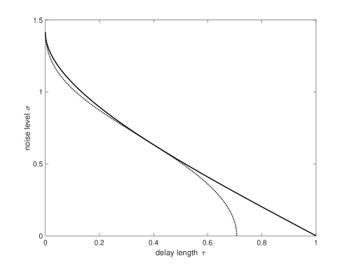
Figure 1. Comparison of sufficient conditions for asymptotic decay of $\mathbb{E}[w^{2}]$ formulated by Theorem 1, solid line, and by [4, Lemma 3.5], dashed line.

Finally, let us refer to [4, Fig. 2] for a comparison of the analytical condition (2.5) to results of systematic Monte Carlo simulations, which indicates that there is still a significant potential for improvement of the analytical result.

Our second result provides a sufficient condition for exponential (monotone) decay of the square mean of solutions of (2.1). Obviously, monotonicity of the solution strongly depends on the initial datum $w_{0}$. Therefore, we consider the generic case of constant, nonzero initial condition $w_{0}\in\mathbb{R}$ in the below Theorem. For notational convenience we define, for $s\geq 0$, the function $G=G(s)$,

(2.6) $$G(s):=\left(\frac{e^{2s}-1}{2s}\right)^{1/2}.$$

Theorem 2.

Let $\tau$, $\sigma\geq 0$ be such that the conditions

(2.7) $$\sigma<e^{-\mu\tau}\sqrt{2\mu-2e^{\mu\tau}}$$

and

(2.8) $$\sigma<-G(\mu\tau)\sqrt{\tau}+\sqrt{G(\mu\tau)^{2}\tau-2G(\mu\tau)\tau+2}$$

are simultaneously verified for some $\mu>1$, with the function $G$ defined in (2.6). Then $\mathbb{E}[w(t)^{2}]$ decays exponentially to zero as $t\to\infty$, where $w=w(t)$ is the solution of (2.1) subject to the constant initial datum $w_{0}\neq 0$.

Obviously, the condition posed by Theorem 2 is not explicit, since it involves a search for $\mu>1$ such that both (2.7) and (2.8) are satisfied. Finding the maximal admissible $\sigma=\sigma(\tau)$ for a given $\tau\geq 0$ in fact means

(2.9) $$\sigma(\tau):=\max_{\mu>1}\min\left\{f_{1}(\tau,\mu),f_{2}(\tau,\mu)\right\},$$

where $f_{1}=f_{1}(\tau,\mu)$ and, resp., $f_{2}=f_{2}(\tau,\mu)$ denote the right-hand sides of (2.7) and, resp., (2.8). It does not seem feasible to find an explicit analytical formula for $\sigma(\tau)$ in (2.9), however, the problem is quite easily approachable numerically. First, let us observe that (2.7) is only satisfiable if $\mu>e^{\mu\tau}$, which requires $\tau<e^{-1}$. Consequently, for each $\tau\in(0,e^{-1})$ we only need to search values of $\mu$ such that $\mu>e^{\mu\tau}$, which represents a bounded interval. The situation is also simplified by the fact that, as revealed by a simple analysis, $f_{2}(\tau,\mu$) is a decreasing function of $\mu$ for any fixed $\tau<e^{-1}$. The result of numerical realization of (2.9) is plotted in Fig. 2, where also the condition for asymptotic decay (2.4) is indicated for comparison. Finally, let us note that for $\tau=0$, the conditions (2.7)–(2.8) collapse to $\sigma^{2}<2$, which is the sharp condition for asymptotic decay in mean square of the (nondelay) geometric Brownian motion. Also the condition $\tau<e^{-1}$ is sharp, since all nontrivial solutions of (1.3) oscillate if $\tau>e^{-1}$.

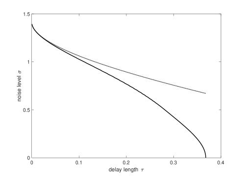
Figure 2. Numerical realization of the sufficient condition for exponential decay of $\mathbb{E}[w^{2}]$ as formulated in Theorem 2, solid line. For comparison, sufficient condition for asymptotic decay given by Theorem 1, dotted line.

3. Asymptotic decay: Proof of Theorem 1

For $p$, $q>0$ and $t>0$ we define the functional

(3.1) $$\mathscr{L}(t):=|w(t)|^{2}+q\int_{t-\tau}^{t}|w(s)|^{2}\mathrm{d}s+p\int_{t-\tau}^{t}\int_{\theta}^{t}|w(s-\tau)|^{2}\mathrm{d}s\mathrm{d}\theta,$$

where $w=w(t)$ is the solution of (2.1)–(2.2); we refer to [5, 16] for an overview of the theory of Lyapunov functionals for systems with delay.

Lemma 1.

Let $\sigma^{2}<2$ and

(3.2) $$\tau<1-\frac{\sigma}{2}\sqrt{4-\sigma^{2}}.$$

Then there exist $p$, $q>0$ and $\kappa>0$ such that

(3.3) $$\frac{\mathrm{d}}{\mathrm{d}t}\mathbb{E}[\mathscr{L}(t)]\leq-\kappa\mathbb{E}[w(t-\tau)^{2}]\qquad\mbox{for }t>\tau.$$

Proof.

We apply the Itô formula to calculate $\mathrm{d}|w(t)|^{2}$. Note that the Itô formula holds in its usual form also for delay stochastic processes, see page 32 in [6] or [9, 10, 3, 12], and with (2.1) it gives

(3.4) $$\mathrm{d}|w(t)|^{2}=2\left(-\widetilde{w}w+\frac{\sigma^{2}}{2}\widetilde{w}^{2}\right)\mathrm{d}t+2\sigma\widetilde{w}w\mathrm{d}B_{t}.$$

Consequently,

$$\mathrm{d}\mathscr{L}(t) = 2\left(-\widetilde{w}w+\frac{\sigma^{2}}{2}\widetilde{w}^{2}\right)\mathrm{d}t+2\sigma\widetilde{w}w\mathrm{d}B_{t}$$

$$\qquad+\;q(w^{2}-\widetilde{w}^{2})\mathrm{d}t+p\left(-\int_{t-\tau}^{t}|w(s-\tau)|^{2}\mathrm{d}s+\tau\widetilde{w}^{2}\right)\mathrm{d}t.$$

For any $\delta>0$ we have

$$-2\widetilde{w}w=-2(\widetilde{w}-w)w-2w^{2}\leq\delta|w-\widetilde{w}|^{2}+(\delta^{-1}-2)w^{2}.$$

Restricting to $t>\tau$, we have for any $\varepsilon>0$,

$$|w-\widetilde{w}|^{2}=\left|\int_{t-\tau}^{t}\mathrm{d}w(s)\right|^{2} \leq \left(\left|\int_{t-\tau}^{t}w(s-\tau)\mathrm{d}s\right|+\sigma\left|\int_{t-\tau}^{t}w(s-\tau)\mathrm{d}B_{s}\right|\right)^{2}$$

$$\leq (1+\varepsilon)\left(\int_{t-\tau}^{t}w(s-\tau)\mathrm{d}s\right)^{2}+(1+\varepsilon^{-1})\sigma^{2}\left(\int_{t-\tau}^{t}w(s-\tau)\mathrm{d}B_{s}\right)^{2}.$$

We take the expectation and use the Jensen inequality and Fubini theorem for the term

$$\mathbb{E}\left[\left(\int_{t-\tau}^{t}w(s-\tau)\mathrm{d}s\right)^{2}\right]\leq\tau\mathbb{E}\left[\int_{t-\tau}^{t}|w(s-\tau)|^{2}\mathrm{d}s\right]=\tau\int_{t-\tau}^{t}\mathbb{E}\left[|w(s-\tau)|^{2}\right]\mathrm{d}s,$$

and the isometry of the Itô integral [11, Theorem 5.8(iii)], for the term

$$\mathbb{E}\left[\left(\int_{t-\tau}^{t}w(s-\tau)\mathrm{d}B_{s}\right)^{2}\right]=\int_{t-\tau}^{t}\mathbb{E}\left[|w(s-\tau)|^{2}\right]\mathrm{d}s.$$

Therefore, we arrive at

$$\mathbb{E}\left[|w-\widetilde{w}|^{2}\right]\leq\left((1+\varepsilon)\tau+(1+\varepsilon^{-1})\sigma^{2}\right)\int_{t-\tau}^{t}\mathbb{E}\left[|w(s-\tau)|^{2}\right]\mathrm{d}s.$$

Minimization of the right-hand side in $\varepsilon>0$ leads to $\varepsilon:=\sigma/\sqrt{\tau}$, and thus

$$\mathbb{E}\left[|w-\widetilde{w}|^{2}\right]\leq\left(\sqrt{\tau}+\sigma\right)^{2}\int_{t-\tau}^{t}\mathbb{E}\left[|w(s-\tau)|^{2}\right]\mathrm{d}s.$$

Consequently, taking the expectation in (3), we obtain

$$\frac{\mathrm{d}}{\mathrm{d}t}\mathbb{E}[\mathscr{L}(t)]\leq\left(\delta^{-1}+q-2\right)\mathbb{E}[w^{2}]+\left(\sigma^{2}+p\tau-q\right)\mathbb{E}[\widetilde{w}^{2}]+\left(\delta(\sqrt{\tau}+\sigma)^{2}-p\right)\int_{t-\tau}^{t}\mathbb{E}\left[|w(s-\tau)|^{2}\right]\mathrm{d}s.$$

With the choice

$$p:=\delta(\sqrt{\tau}+\sigma)^{2},\qquad q:=2-\delta^{-1}$$

we arrive at

$$\frac{\mathrm{d}}{\mathrm{d}t}\mathbb{E}[\mathscr{L}(t)]\leq\Bigl{(}\sigma^{2}+\delta\tau(\sqrt{\tau}+\sigma)^{2}+\delta^{-1}-2\Bigr{)}\mathbb{E}[\widetilde{w}^{2}].$$

Minimization of the right-hand side with respect to $\delta>0$ gives $\delta:=\left(\tau(\sqrt{\tau}+\sigma)^{2}\right)^{-1/2}$ and

$$\frac{\mathrm{d}}{\mathrm{d}t}\mathbb{E}[\mathscr{L}(t)]\leq-\kappa\mathbb{E}[\widetilde{w}^{2}]$$

with

(3.6) $$-\kappa:=\left(\sigma+\sqrt{\tau}\right)^{2}+\tau-2.$$

Finally, a simple calculation reveals that if $\sigma^{2}<2$, then $\kappa>0$ if and only if (3.2) is satisfied. It is easily checked that then $p$ and $q$ are both positive. ∎

Proof of Theorem 1. Obviously, with the bounded initial datum (2.2), we have $\mathbb{E}[\mathscr{L}(\tau)]<+\infty$ due to (3). An integration of (3.3) in time gives, for $t>\tau$,

(3.7) $$\mathbb{E}[w(t)^{2}] \leq \mathbb{E}[\mathscr{L}(t)]=\mathbb{E}[\mathscr{L}(\tau)]+\int_{\tau}^{t}\frac{\mathrm{d}}{\mathrm{d}s}\mathbb{E}[\mathscr{L}(s)]\mathrm{d}s$$

$$\leq \mathbb{E}[\mathscr{L}(\tau)]-\kappa\int_{\tau}^{t}\mathbb{E}[w(s-\tau)^{2}]\mathrm{d}s,$$

with $\kappa>0$ given by (3.6). Consequently, $\mathbb{E}[w(t)^{2}]$ is uniformly bounded by $\mathbb{E}[\mathscr{L}(\tau)]$ for $t>\tau$. Taking the expectation in (3.4) and using the Cauchy-Schwartz inequality, we have

$$\frac{\mathrm{d}}{\mathrm{d}t}\mathbb{E}[w(t)^{2}] = -2\mathbb{E}[w\widetilde{w}]+\sigma^{2}\mathbb{E}[\widetilde{w}^{2}]$$

$$\leq \mathbb{E}[w^{2}]+(1+\sigma^{2})\mathbb{E}[\widetilde{w}^{2}],$$

which gives uniform boundedness of $\frac{\mathrm{d}}{\mathrm{d}t}\mathbb{E}[w(t)^{2}]$ for $t>2\tau$. Moreover, we note that due to (3.7) the integral $\int_{\tau}^{t}\mathbb{E}[w(s-\tau)^{2}]\mathrm{d}s$ is convergent as $t\to\infty$. Barbalat’s lemma [2] then implies that $\lim_{t\to\infty}\mathbb{E}[w(t)^{2}]=0$ and concludes the proof of Theorem 1.

4. Exponential decay: Proof of Theorem 2

In this section we assume that $w=w(t)$ is a solution of (2.1) subject to the deterministic constant initial datum $w_{0}\neq 0$, and we introduce the notation

$$y(t) := \mathbb{E}[w^{2}(t)/2]\qquad\mbox{for }t\geq 0,$$

$$:= w_{0}^{2}/2\qquad\mbox{for }t<0.$$

Lemma 2.

Let $\sigma^{2}\leq 2$. If for some $\mu>1$ the condition

(4.2) $$2e^{\mu\tau}+\sigma^{2}e^{2\mu\tau}\leq 2\mu$$

is satisfied, then for all $t\in\mathbb{R}$ and $s>0$,

(4.3) $$e^{-2\mu s}y(t)<y(t-s)<e^{2\mu s}y(t).$$

Proof.

An application of the Itô formula gives

$$\frac{\mathrm{d}{w^{2}}}{2}=\left(-\widetilde{w}w+\frac{\sigma^{2}}{2}\widetilde{w}^{2}\right)\mathrm{d}t+\sigma\widetilde{w}w\mathrm{d}B_{t},$$

and taking expectation, we have for $t>0$,

(4.4) $$\dot{y}=\mathbb{E}\left[-\widetilde{w}w+\frac{\sigma^{2}}{2}\widetilde{w}^{2}\right].$$

With the constant initial datum $w_{0}\in\mathbb{R}$, we obtain for $t=0$,

$$\dot{y}(0+)=\left(-1+\frac{\sigma^{2}}{2}\right)w_{0}^{2},$$

where $\dot{y}(0+)$ denotes the right-hand side derivative of $y$ at $t=0$. Consequently, since by assumption $\mu>1$,

$$\left|\frac{\dot{y}(0+)}{y(0)}\right|=2-\sigma^{2}<2\mu.$$

Due to nonzero constant initial datum and the continuity of $y(t)$ and $\dot{y}(t)$ for $t>0$, there exists $T>0$ such that

(4.5) $$\left|\frac{\dot{y}(t)}{y(t)}\right|<2\mu\qquad\mbox{for }t<T.$$

We claim that (4.5) holds for all $t\in\mathbb{R}$, i.e., that $T=+\infty$.

For contradiction, assume that $T<+\infty$, then again by continuity we have

(4.6) $$|\dot{y}(T)|=2\mu y(T).$$

Integrating (4.5) on the time interval $(T-s,T)$ with $s>0$ yields

(4.7) $$y(T-s)<e^{2\mu s}y(T).$$

With (4.4) and the Cauchy-Schwartz inequality with $\varepsilon>0$ we have for $t>0$,

$$|\dot{y}|\leq\mathbb{E}\left[|\widetilde{w}||w|\right]+\sigma^{2}\widetilde{y}\leq 2\sqrt{\widetilde{y}}\sqrt{y}+\sigma^{2}\widetilde{y}\leq\varepsilon y+\left(\varepsilon^{-1}+\sigma^{2}\right)\widetilde{y}.$$

Using (4.7) with $s:=\tau$ gives $y(T-\tau)<e^{2\mu\tau}y(T)$, so that

$$|\dot{y}(T)|<\Bigl{(}\varepsilon+\left(\varepsilon^{-1}+\sigma^{2}\right)e^{2\mu\tau}\Bigr{)}y(T),$$

and minimization of the right-hand side with respect to $\varepsilon>0$ gives

$$|\dot{y}(T)|<\left(2e^{\mu\tau}+\sigma^{2}e^{2\mu\tau}\right)y(T).$$

Finally, assumption (4.2) gives

$$|\dot{y}(T)|<2\mu y(T),$$

which is a contradiction to (4.6). Consequently, (4.5) holds for all $t\in\mathbb{R}$, and an integration on the interval $(t-s,t)$, taking into account the constant initial datum, implies (4.3). ∎

Lemma 3.

Let the condition (4.2) of Lemma 2 be satisfied for some $\mu>1$. Then we have, along the solutions of (2.1),

(4.8) $$\dot{y}<2\left[\left(\sqrt{\tau}+\sigma\right)\left(\frac{e^{2\mu\tau}-1}{2\mu}\right)^{1/2}+\frac{\sigma^{2}}{2}-1\right]\widetilde{y},$$

for $t>0$.

Proof.

Referring to (4.4) we have for $t>0$,

(4.9) $$\dot{y}=\mathbb{E}\left[-\widetilde{w}w\right]+\frac{\sigma^{2}}{2}\mathbb{E}\left[\widetilde{w}^{2}\right],$$

and, with the Cauchy-Schwartz inequality,

$$\mathbb{E}\left[-\widetilde{w}w\right]=\mathbb{E}\left[(\widetilde{w}-w)\widetilde{w}\right]-\mathbb{E}\left[\widetilde{w}^{2}\right]\leq\Bigl{(}\mathbb{E}\left[|w-\widetilde{w}|^{2}\right]\Bigr{)}^{1/2}\Bigl{(}\mathbb{E}\left[\widetilde{w}^{2}\right]\Bigr{)}^{1/2}-\mathbb{E}\left[\widetilde{w}^{2}\right].$$

If $t>\tau$, we have for any $\varepsilon>0$,

$$|w-\widetilde{w}|^{2}=\left|\int_{t-\tau}^{t}\mathrm{d}w(s)\right|^{2} = \left(\int_{t-\tau}^{t}w(s-\tau)\mathrm{d}s+\sigma\int_{t-\tau}^{t}w(s-\tau)\mathrm{d}B_{s}\right)^{2}$$

$$\leq (1+\varepsilon)\left(\int_{t-\tau}^{t}w(s-\tau)\mathrm{d}s\right)^{2}+(1+\varepsilon^{-1})\sigma^{2}\left(\int_{t-\tau}^{t}w(s-\tau)\mathrm{d}B_{s}\right)^{2}.$$

As in the proof of Lemma 1, we take the expectation and use the Jensen inequality, Fubini theorem and isometry of the Itô integral to obtain

(4.10) $$\mathbb{E}\left[|w-\widetilde{w}|^{2}\right]\leq\left((1+\varepsilon)\tau+(1+\varepsilon^{-1})\sigma^{2}\right)\int_{t-\tau}^{t}\mathbb{E}\left[|w(s-\tau)|^{2}\right]\mathrm{d}s.$$

If $0<t\leq\tau$, we have, due to the constant initial condition,

$$|w-\widetilde{w}|^{2}=\left|\int_{t-\tau}^{t}\mathrm{d}w(s)\right|^{2}=\left(\int_{0}^{t}w(s-\tau)\mathrm{d}s+\sigma\int_{0}^{t}w(s-\tau)\mathrm{d}B_{s}\right)^{2},$$

and a trivial modification of the above estimates gives (4.10) again. Consequently, (4.10) holds for all $t>0$, with the constant initial datum $w_{0}$ being extended to the interval $[-2\tau,0]$. Minimization of the right-hand side in $\varepsilon>0$ leads to $\varepsilon:=\sigma/\sqrt{\tau}$, and thus

$$\mathbb{E}\left[|w-\widetilde{w}|^{2}\right]\leq\left(\sqrt{\tau}+\sigma\right)^{2}\int_{t-\tau}^{t}\mathbb{E}\left[|w(s-\tau)|^{2}\right]\mathrm{d}s.$$

An application of Lemma 2 gives

$$\int_{t-\tau}^{t}\mathbb{E}\left[|w(s-\tau)|^{2}\right]\mathrm{d}s=2\int_{t-\tau}^{t}y(s-\tau)\mathrm{d}s<2y(t-\tau)\int_{0}^{\tau}e^{2\mu s}\mathrm{d}s=\frac{e^{2\mu\tau}-1}{\mu}\widetilde{y}.$$

Consequently, we have

$$\mathbb{E}\left[-\widetilde{w}w\right]<2\left[\left(\sqrt{\tau}+\sigma\right)\left(\frac{e^{2\mu\tau}-1}{2\mu}\right)^{1/2}-1\right]\widetilde{y},$$

and inserting this into (4.9) immediately gives (4.8). ∎

Proof of Theorem 2. Lemmata 2 and 3 assert that $y(t)=\mathbb{E}[w(t)^{2}/2]$ is monotonically decaying if condition (4.2) is satisfied for some $\mu>1$ and if

(4.11) $$\left(\sqrt{\tau}+\sigma\right)\left(\frac{e^{2\mu\tau}-1}{2\mu}\right)^{1/2}+\frac{\sigma^{2}}{2}<1.$$

A simple calculation reveals that (4.2) is equivalent to (2.7), while (4.11) is equivalent to (2.8). Then, a combination of (4.3) with $s:=\tau$ and (4.8) yields

$$\dot{y}(t)<\left[\left(\sqrt{\tau}+\sigma\right)\left(\frac{e^{2\mu\tau}-1}{2\mu}\right)^{1/2}+\frac{\sigma^{2}}{2}-1\right]e^{-2\mu\tau}y(t),$$

for $t>0$, which implies exponential decay of $y=y(t)$ in time.

Authors’ addresses: Jan Haskovec, King Abdullah University of Science and Technology, 23955 Thuwal, KSA. e-mail: jan.haskovec@kaust.edu.sa.

References

- [1] J. Appleby, X. Mao, and M. Riedle: Geometric Brownian motion with delay: mean square characterisation, Proceedings of The American Mathematical Society 137 (2009), pp. 339–348. Zbl 1156.60045, MR2439458.
- [2] I. Barbalat: Systèmes d’équations différentielles d’oscillations nonlinéaires. Rev. Math. Pures Appl. 4, 2 (1959), 267–270. Zbl 0090.06601, MR0111896.
- [3] L. El’sgol’ts, and S. Norkin, translated by J. Casti: Introduction to the theory and application of differential equations with deviating arguments, Academic Press, New York (1973). Zbl 0287.34073, MR0352647.
- [4] R. Erban, J. Haskovec and Y. Sun: A Cucker-Smale model with noise and delay, SIAM J. Appl. Math. 76 (2016), pp. 1535–1557. Zbl 1345.60063, MR3534479.
- [5] E. Fridman: Tutorial on Lyapunov-based methods for time-delay systems, European Journal of Control 20 (2014), pp. 271–283. Zbl 1403.93158, MR3283869.
- [6] S. Gillouzic: Fokker-Planck approach to stochastic delay differential equations, Thesis, Ottawa, Canada (2000).
- [7] I. Gyori and G. Ladas: Oscillation Theory of Delay Differential Equations with Applications, Oxford Science Publications, Clarendon Press, Oxford (1991). Zbl 0780.34048, MR1168471.
- [8] J. Hull: Options, Futures, and other Derivatives. Prentice-Hall International Editions. Upper Saddle River, NJ (2003). Zbl 1087.91025.
- [9] V. Kolmanovskii, and A. Myshkis: Applied theory of functional differential equations, Dordrecht: Kluwer Academic Publishers (1992). Zbl 0785.34005, MR1256486.
- [10] V. Kolmanovskii, and A. Myshkis: Introduction to the Theory and Applications of Functional Differential Equations. Dordrecht: Kluwer Academic Publishers (1999). Zbl 0917.34001, MR1680144.
- [11] X. Mao: Stochastic Differential Equations and Applications. Second Edition. Horwood Publishing Limited, Chichester (1997). Zbl 1138.60005, MR2380366.
- [12] X. Mao: Stability and stabilisation of stochastic differential delay equations, IET Control Theory Appl. 1 (6), pp. 1551–1566 (2007). doi: 10.1049/iet-cta:20070006.
- [13] S-E. A. Mohammed and M. K. R. Scheutzow: Lyapunov exponents of linear stochastic functional differential equations. II: Examples and case studies. Ann. Probab., 25, 3, 1210–1240 (1997). Zbl 0885.60043, MR1457617.
- [14] B. Øksendal: Stochastic Differential Equations. An introduction with applications. Sixth edition, Universitext, Springer-Verlag, Berlin (2003). Zbl 1025.60026, MR2001996.
- [15] H. Smith: An Introduction to Delay Differential Equations with Applications to the Life Sciences. Springer New York Dordrecht Heidelberg London (2011). Zbl 1227.34001, MR2724792.
- [16] J. Sun, and J. Chen: A survey on Lyapunov-based methods for stability of linear time-delay systems. Frontiers of Computer Science 11 (2017), pp. 555–567. Zbl 1405.34046.