Planning from Images with Deep Latent Gaussian Process Dynamics

Abstract

Planning is a powerful approach to control problems with known environment dynamics. In unknown environments the agent needs to learn a model of the system dynamics to make planning applicable. This is particularly challenging when the underlying states are only indirectly observable through images. We propose to learn a deep latent Gaussian process dynamics (DLGPD) model that learns low-dimensional system dynamics from environment interactions with visual observations. The method infers latent state representations from observations using neural networks and models the system dynamics in the learned latent space with Gaussian processes. All parts of the model can be trained jointly by optimizing a lower bound on the likelihood of transitions in image space. We evaluate the proposed approach on the pendulum swing-up task while using the learned dynamics model for planning in latent space in order to solve the control problem. We also demonstrate that our method can quickly adapt a trained agent to changes in the system dynamics from just a few rollouts. We compare our approach to a state-of-the-art purely deep learning based method and demonstrate the advantages of combining Gaussian processes with deep learning for data efficiency and transfer learning.

1 Introduction

Reinforcement learning (RL) has shown success for a number of applications, including Atari games (Mnih et al., 2015), robotic manipulation (Gu et al., 2017), navigation and reasoning tasks (Oh et al., 2016), and machine translation (II et al., 2014). Many such results were obtained with model-free deep RL in which the agent directly learns a policy function in the form of a neural network by interacting with the environment. However, such approaches commonly require a large number of interactions, which often hinders their application to real-world tasks: Performing actions in real environments, such as driving a vehicle or moving a robot, can be orders of magnitude slower than performing an update of the policy model, and mistakes can carry real-world costs.

Model-based RL is a promising direction to reduce this sample complexity. In model-based RL, the agent acquires a predictive model of the world and uses the model to make decisions. This offers several potential benefits over model-free approaches. First, learning a transition model enables the agent to leverage a richer training signal by using the observed transition instead of just propagating a scalar reward. Further, the learned dynamics can be independent of the specified task and could therefore potentially be transferred to other tasks in the same environment. Finally, instead of learning a policy function the agent can use the learned environment for planning to choose its actions. For environments with only a few state variables, PILCO (Deisenroth and Rasmussen, 2011) achieves remarkable sample efficiency. A crucial component is its use of Gaussian processes to model the system dynamics, which allows PILCO to include the uncertainty of the transition model into its policy search. However, in many problems of interest the underlying state of the world is only indirectly observable through images. In order to enable fast planning, the agent can learn low-dimensional state representations and model the system dynamics in the learned latent space. Models of this type have been successfully applied to simple tasks such as balancing cartpoles and controlling 2-link arms (Watter et al., 2015; Banijamali et al., 2018). However, model-based RL approaches are generally known to lag behind model-free methods in asymptotic performance for problems of this type. Recently, PlaNet (Hafner et al., 2019) was able to match top model-free algorithms in complex image-based domains. PlaNet learns environment dynamics from pixels and chooses actions through online planning in latent space. Notably, all components in PlaNet are modeled through neural networks.

1.1 Contributions

• We combine Gaussian processes (GPs) with neural networks to learn latent dynamics models from visual observations. All parts of the proposed deep latent Gaussian process dynamics (DLGPD) model can be trained jointly by optimizing a lower bound on the likelihood of transitions in image space.

• We integrate the learned system dynamics with learning a reward function and use the models for model-predictive control. In our experiments, the predictions of the learned dynamics model enable the agent to successfully solve an inverted pendulum swing-up task.

• We demonstrate that the latent Gaussian process dynamics model allows the agent to quickly adapt to environments with modified system dynamics from only few rollouts. Our approach compares favorably to the purely deep-learning based baseline PlaNet (Hafner et al., 2019) in this transfer learning experiment.

1.2 Related Work

Bayesian nonparametric Gaussian process models (Rasmussen and Williams, 2006) are a popular choice for dynamics models in reinforcement learning (RL) (Wang et al., 2005; Rasmussen and Kuss, 2003; Ko et al., 2007; Deisenroth et al., 2009). When the low-dimensional states of the environment are available to the agent, PILCO (Deisenroth and Rasmussen, 2011) achieves remarkable sample efficiency and is able to solve a swing-up task in a real cart-pole system with only 17.5 seconds of interaction. Deep PILCO (Gal et al., 2016) replace GPs in PILCO with Bayesian neural networks to learn the dynamics model. The method is not demonstrated to learn an embedding of high dimensional image observations but directly operates on low-dimensional state representations.

Model-free deep RL algorithms have shown good performance in image-based domains (Mnih et al., 2015; Lillicrap et al., 2016), but they commonly require a large number of interactions. On the other hand, model-based RL can often be more data-efficient. Many such algorithms learn low-dimensional abstract state representations (Lesort et al., 2018) and model the system dynamics in the learned latent space (Fraccaro et al., 2017; Karl et al., 2017). Some approaches such as E2C (Watter et al., 2015), RCE (Banijamali et al., 2018) or SOLAR (Zhang et al., 2019) learn locally-linear latent transitions and plan for actions based on the linear quadratic regulator (LQR). In comparison, we learn a non-local, non-linear dynamics model to select actions by planning in latent space. PlaNet (Hafner et al., 2019) learns a recurrent encoder and a latent neural transition model to efficiently plan in latent space. All components of PlaNet are modeled through deep neural networks. We propose to model state transitions with GPs to reduce the number of model parameters, provide better uncertainty estimates, and generally increase the data-efficiency.

Our formulation provides a data-efficient way to transfer a learned dynamics model to different system dynamics. Closely related are meta-learning approaches that also learn to transfer between different properties for the same task (e.g. (Al-Shedivat et al., 2018; Killian et al., 2017; Saemundsson et al., 2018)). While our models are not specifically trained for transferability, it is an inherent property of our formulation.

2 Learning Deep Latent Gaussian Process Dynamics for Control

We propose a novel approach for learning system dynamics from high-dimensional image observations. We combine the advantages of deep representation learning with Gaussian processes for data-efficient Bayesian modeling of the latent system dynamics. For control, the agent requires a model of the dynamical system as well as a reward model and an encoder to infer its belief over latent states from observations. In the following, we formulate our learning framework which learns all these components jointly from image observations and environment interactions. We also propose our approach for model-predictive control and transfer learning based on our learned models.

2.1 Deep Gaussian Process State Space Models

We consider dynamical systems with latent states $s\in\mathbb{R}^{D}$, actions $a\in\mathbb{R}^{K}$, and observations $o\in\mathbb{R}^{M}$. We call $p(s_{t+1}\>|\>s_{t},a_{t})=\mathcal{N}(s_{t+1}\>|\>f(s_{t},a_{t}),\Sigma_{f})$ the state-transition model with state-transition function $f$ for discrete time steps $t\in\mathbb{N}$. The observation model $p(o_{t}\>|\>s_{t})$ is associated with the observation function $g$, where $g(s_{t})$ is the expected measurement. In addition, we consider a control task specified by a reward model $p(r_{t+1}\>|\>s_{t},a_{t})=\mathcal{N}(r_{t+1}\>|\>h(s_{t},a_{t}),\Sigma_{r})$ with reward function $h(s_{t},a_{t})$ and noise $\Sigma_{r}$. Figure 1 illustrates the generative process.

A possible approach to learn the above models would be to restrict $f$, $g$, and $h$ to families of parametric functions such as deep neural networks. However, these usually require large training datasets in order to avoid overfitting. On the other hand, Bayesian nonparametric methods such as GPs often perform well with smaller datasets. We combine their respective properties and choose different types of methods for the different model components. First, we model the transition function through a GP $f\sim\mathcal{GP}(\mu_{f}(\cdot),k_{f}(\cdot,\cdot))$, with mean function $\mu_{f}:(s_{t},a_{t})\mapsto s_{t}$ and radial basis function (RBF) kernel $k_{f}$. For state dimensionality $D>1$ we model each output dimension of the transition function with a conditionally independent GP. Similarly, we chose a GP reward model $h\sim\mathcal{GP}(r_{\text{min}},k_{h}(\cdot,\cdot))$ where $r_{\text{min}}$ is the minimal reward observed in the collected training data and $k_{h}$ the RBF kernel. Convolutional neural networks are currently the state-of-the-art method for learning and extracting low-dimensional latent encodings from images. We model the observation function $g$ with a transposed-convolutional network. For the observation likelihood $p(o_{t}\>|\>s_{t})$ we use an approximate Bernoulli likelihood of $o_{t}\in[0,1]^{M}$ under the expected measurement $g(s_{t})$. Finally, to infer approximate state posteriors from observations we learn a probabilistic encoder of the form $q(s_{t}\>|\>o_{t})\sim\mathcal{N}\left(s_{t}\>|\>\mu(o_{t}),\sigma(o_{t})^{2}\cdot I\right)$ with vector-valued $\mu(\cdot)$ and $\sigma(\cdot)$ parametrized by a convolutional neural network.

To enable state inference from a single observation, we consider observations $o_{t}$ to consist of two subsequent frames $[i_{t-1},i_{t}]$ (see fig. 1). This allows for approximate inference of positions and velocities, which is sufficient to fully describe the state of the pendulum task considered in our experiments. Note that for different environments with more complex states or with long-term dependencies it might not be possible to infer a state from two subsequent frames and hence be necessary to choose a more general encoder $q(s_{t}\>|\>o_{\leq t},a_{<t})$, e.g. by filtering through a recurrent encoder (Hafner et al., 2019).

2.2 Training Objective

We jointly learn all parameters of the model, which include the weights of the neural networks and the hyperparameters of the GP, from interactions with the environment. Consider transitions $(o_{t},a_{t},o_{t+1},r_{t+1})$ collected by interacting with the environment. To model the covariances of individual data points we group the observed transitions into a joint training dataset $\mathcal{D}=\left\{O,A,O^{\prime},R^{\prime}\right\}$, with $O=\{o_{1},\dots,o_{T-1}\}$, $A=\{a_{1},\dots,a_{T-1}\}$, $O^{\prime}=\{o_{2},\dots,o_{T}\}$, and $R^{\prime}=\{r_{2},\dots,r_{T}\}$. We further define latent states $S=\{s_{1},\dots,s_{T-1}\}$ and $S^{\prime}=\{s_{2},\dots,s_{T}\}$.

With the encoder $q(s_{t}\>|\>o_{t})$ we can express the likelihood over latent states as $q(S\>|\>O)=\prod_{t=1}^{T-1}q(s_{t}\>|\>o_{t})$ and $q(S^{\prime}\>|\>O^{\prime})=\prod_{t=2}^{T}q(s_{t}\>|\>o_{t})$. Similarly, with our observation model we can write $p(O\>|\>S)=\prod_{t=1}^{T-1}p(o_{t}\>|\>s_{t})$ and $p(O^{\prime}\>|\>S^{\prime})=\prod_{t=2}^{T}p(o_{t}\>|\>s_{t})$. Finally, since we model the state transitions and the rewards through GPs, the densities $p(S^{\prime}\>|\>S,A)$ and $p(R^{\prime}\>|\>S,A)$ are from multivariate Gaussian distributions which we do not factorize over individual transitions.

We marginalize the data likelihood $p(O^{\prime},R^{\prime}\>|\>O,A)$ in the following way:

$$p(O^{\prime},R^{\prime}\>|\>O,A) =\iint p(O^{\prime}\>|\>S^{\prime})\,p(S^{\prime}\>|\>S,A)\,p(R^{\prime}\>|\>S,A)\,q(S\>|\>O)\,\mathrm{d}S\,\mathrm{d}S^{\prime}$$ (1)

$$=\mathbb{E}_{q(S^{\prime}\>|\>O^{\prime})q(S\>|\>O)}\left[p(O^{\prime}\>|\>S^{\prime})\,p(S^{\prime}\>|\>S,A)\,p(R^{\prime}\>|\>S,A)\,\frac{1}{q(S^{\prime}\>|\>O^{\prime})}\right].$$ (2)

With Jensen’s inequality we obtain our training objective as a lower bound on the log-likelihood:

$$\begin{split}\log p(O^{\prime},R^{\prime}\>|\>O,A)&\geq\underbrace{\mathbb{E}_{q(S^{\prime}\>|\>O^{\prime})}\left[\log p(O^{\prime}\>|\>S^{\prime})\right]}_{\text{(I): Reconstruction}}+\underbrace{\mathbb{E}_{q(S^{\prime}\>|\>O^{\prime})}\left[-\log q(S^{\prime}\>|\>O^{\prime})\right]}_{\text{(II): Encoder regularization}}\\ &\quad+\underbrace{\mathbb{E}_{q(S^{\prime}\>|\>O^{\prime})q(S\>|\>O)}\left[\log p(S^{\prime}\>|\>S,A)\right]}_{\text{(III): State transitions}}+\underbrace{\mathbb{E}_{q(S\>|\>O)}\left[\log p(R^{\prime}\>|\>S,A)\right]}_{\text{(IV): Reward}}.\end{split}$$ (3)

We refer to appendix A for a more detailed derivation. The four terms of the derived lower bound have readily interpretable roles: The first term (I) describes a (negative) reconstruction loss. Since the decoder parametrizes a Bernoulli distribution over pixel values, it is equivalent to the negative binary cross-entropy loss. The second term (II) corresponds to the differential entropy of the encoder $q(s_{t}\>|\>o_{t})$ and can be interpreted as a regularization term on the encoder. For multivariate Gaussian distribution with diagonal covariance matrix $\Sigma=\operatorname{diag}([\sigma_{1}^{2},\dots,\sigma_{D}^{2}])$, the differential entropy is proportional to $\sum_{i}\log\left(\sigma_{i}\right)$. Thus, the term prevents vanishing variances. Term (III) describes the likelihood of transitions in latent state space in expectation over the encoder. Since the state transitions are modeled with a GP, the inner likelihood corresponds to the so-called marginal log-likelihood (MLL), which is a common training objective for hyperparameter selection in Gaussian process regressions (Rasmussen and Williams, 2006). Similarly, (IV) shows the MLL for the reward-GP, again in expectation over the encoder. For the loss terms (I), (III), and (IV) we estimate the outer expectations using a single reparametrized sample (Kingma and Welling, 2014; Rezende et al., 2014). The differential entropy (II) can be computed analytically, since the encoder provides a multivariate Gaussian distribution.

For computational tractability, we maximize the lower bound in eq. 3 over batched subsamples of our training dataset, which for Gaussian processes can be theoretically justified by the subset-of-data-approximation (Liu et al., 2018; Hayashi et al., 2019). To improve training stability we normalize the encoded states $(S,S^{\prime})$ batch-wise to zero mean and unit variance before passing them to the transition- and reward GPs. For testing we compute fixed normalization parameters from the full training dataset. Before decoding predicted states the normalization is reversed. Furthermore, we limit the signal-to-noise ratio of the RBF kernels of transition and reward GPs by minimizing an additional penalty term (see appendix B).

2.3 Posterior Inference with Latent Gaussian Processes

To compute the predictive distributions of the transition model and reward model, the GPs need to be conditioned on evidence. With the training data $\mathcal{D}=\left\{O,A,O^{\prime},R^{\prime}\right\}$ and the encoder $q(s\>|\>o)$ we compute latent states $(S,S^{\prime})$, using reparametrized samples (Rezende et al., 2014; Kingma and Welling, 2014) of the predicted distribution as the state representations. For an arbitrary but known state $s_{t}^{*}$ and action $a_{t}^{*}$ we then obtain the posteriors $p\left(s_{t+1}^{*}\>|\>s_{t}^{*},a_{t}^{*},\left((S,A),S^{\prime}\right)\right)$ and $p\left(r_{t+1}^{*}\>|\>s_{t}^{*},a_{t}^{*},\left((S,A),R^{\prime}\right)\right)$ through standard posterior GP inference (Rasmussen and Williams, 2006).

[Image pairs as observations] [Generative model] [Prediction with DLGPD]

Figure 1: Graphical models depicting relationships between random variables in DLGPD, showing (a) the relation between image frames and observations, (b) the generative model we assume, (c) predicting states and rewards.

2.4 Model-Predictive Control

We employ our learned system dynamics for model-predictive control (MPC) (Garcia et al., 1989). Key ingredients for MPC are our learned transition and reward models as well as the encoder which infers latent states from image observations. The observation model is not required for planning. Fig. 1 illustrates prediction with our probabilistic model. We use the cross entropy method (CEM) (Rubinstein, 1996; de Boer et al., 2005) to search for the action sequence that maximizes the expected sum of rewards $\mathbb{E}\left[\sum_{t=1}^{T}r_{t}\right]$. Starting from the mean state encoding of the most recent observation, we compute a state trajectory by forward-propagating the predicted mean. We then approximate the expected reward by averaging the mean prediction of the reward model for 5 samples of the marginal state distribution for every timestep.

3 Experiments

We demonstrate our learning-based control approach on the inverted pendulum (OpenAI Gym Pendulum-v0 (Brockman et al., 2016)), a classical problem of optimal control and continuous reinforcement learning. The goal of this task is to swing-up an inverted pendulum from its resting (hanging-down) position. Due to bounds on the motor torques, a straight upswing of the pendulum is not possible, and the agent has to plan multiple swings to reach and balance the pendulum around the upward equilibrium.

For data collection we excite the system with uniformly sampled random actions $a_{t}\sim\mathcal{U}([-2,2])$. We initialize the system’s state with angles $\theta_{0}\sim\mathcal{U}([-\pi,\pi])$ and angular velocities $\dot{\theta}_{0}\sim\mathcal{U}([-8,8])$. We collect 500 rollouts for training and 3 pools of evidence rollouts, containing 200 rollouts each. Each rollout contains $28$ transitions.

We represent latent states as 3-dimensional real vectors $s_{t}\in\mathbb{R}^{3}$. The observations consist of two subsequent images stacked channel-wise, with image size $64\times 64$ pixels and RGB color channels. We model the probabilistic encoder $q(s_{t}\>|\>o_{t})$ by a convolutional neural network with two output heads for mean and standard deviation. The decoder $p(o_{t}\>|\>s_{t})$ mapping from the latent space to the observation space is implemented by a transposed-convolutional neural network. For more details on the architecture, see appendix D.

For implementation, we use PyTorch (Paszke et al., 2019) and GPyTorch (Gardner et al., 2018).

3.1 Training

The lengthscales of the RBF kernel are initialized as $l=\operatorname{softplus}(0)\approx 0.693$. The outputscales of the transition GPs are initialized to $\alpha^{2}=1$, the output noise variances to $\sigma^{2}=0.2$. We pose $\operatorname{Gamma}(1,5)$ priors on the outputscales and lower bound the outputscales to $10^{-2}$. For the reward GP, the outputscale $\alpha_{\mathrm{reward}}^{2}$ is initialized to the variance of the rewards in the first batch, the output noise variance to $0.2\cdot\alpha_{\mathrm{reward}}^{2}$. All output noise variances are lower bounded by $\alpha^{2}\cdot 10^{-3}$. The prior mean function for the reward GP is set constant as the minimum of all collected rewards, to predict a minimal reward for unseen regions of the state space. All parameters of our model are jointly optimized with Adam (Kingma and Ba, 2014), with a learning rate of $10^{-3}$ and a batch-size of $1024$. To encourage the encoder to learn an embedding for the forward modelling task, we stop gradients from the reward model to the encoder. We train all models for 2000 epochs. To observe the effect of neural network initialization and training data shuffling, we report control performance on three separately trained models.

We train PlaNet on the same training data like our model ($500$ pendulum rollouts with random initialization and random actions), plus additionally $200$ rollouts which is the maximum number of evidence rollouts we use, which gives $700$ rollouts in total. Based on the best average performance on 5 validation rollouts, we choose a model after 3.8 million steps of training. This model serves as the base model for fine-tuning on data from modified environments. For fine-tuning, we evaluate all models every 20k steps for the first 100k steps and every 100k steps for up to 1 million steps, and report results for models where the mean performance is best.

3.2 Model-Based Control

Performance on the swingup task is evaluated on a system randomly initialized with angle $\theta_{0}\sim\mathcal{U}([\pi-0.05,\pi+0.05])$ (pole hanging downwards) and angular velocity $\dot{\theta}_{0}\sim\mathcal{U}([-0.05,0.05])$, based on the achieved cumulative reward over $150$ steps. In order to apply the DLGPD model on prediction and control tasks, the transition and reward GPs have to be conditioned on encoded observations, actions and rewards collected from previous environment interactions. For this we use subsets of rollouts (between 10 and 200 rollouts) from the evidence pools. We use CEM for planning (see section 2.4) with a planning horizon of 20 steps. We report results for 3 control trials on 3 trained models conditioned on a subset of each of the 3 evidence pools (i.e. 27 runs per subset size). The control performance results in terms of cumulative reward are depicted in fig. 2(a). We observe that our approach achieves higher average cumulative reward than PlaNet in this environment already for a small set of evidence rollouts ($\geq 20$). Fig. 3 shows a learned latent embedding and a trajectory followed by the CEM planner.

3.3 Transfer Learning

By modeling the state transitions through a GP, we can learn new state-transition functions of systems with different dynamical properties in a very data-efficient way, as long as the other model components (observation model, reward model, encoder) can be re-used. In particular, we observed that the agent does not require additional training and that it is sufficient to replace the evidence in the transition GP (see section 2.3) with new data of the modified environment, e.g. collected by following a random policy. In the following, we investigate the sample efficiency of our model for adapting to environments with changed physical parameters using new random rollouts. We compare our approach with PlaNet (Hafner et al., 2019) which needs to be fine-tuned on the same rollouts.

To evaluate adaptation capabilities to environments with changed intrinsic properties, we derive three variants of the Pendulum-v0 environment. For the inverted action environment, we flip the sign of the action before passing it to the original environment. Second, we make the pole lighter by reducing its mass from $m=1$ to $m=0.2$; we also increase the pole’s weight to $m=1.5$. Results of PlaNet variants and DLGPD conditioned on evidence from the modified and the original environments (matching/mismatching) are shown in fig. 2(b-d). For inverted actions, our approach achieves significantly higher cumulative reward even for a small number of rollouts in the evidence. PlaNet clearly performs less well with the same amount of training data. With a lower mass than the original pendulum, MPC with both modelling approaches still achieves the swing-up without additional data. For increased mass, our approach achieves higher cumulative reward than PlaNet with only a few extra rollouts. In addition to the cumulative reward, we also evaluated our experiments with respect to the ratio of successful rollouts (see appendix C).

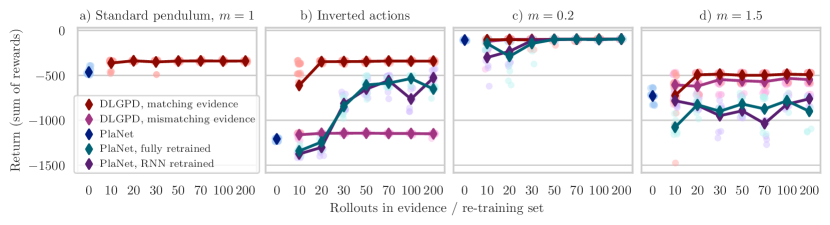
Figure 2: Cumulative rewards for PlaNet and our DLGPD model for swing-up of the inverted pendulum in different settings. For the detailed discussion see section 3.2 for (a) and section 3.3 for (b-d).

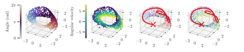
Figure 3: Visualizing the 3-dimensional latent space of the learnt embedding. States are colored according to true physical states of the pendulum (angle and angular velocity). On the two rightmost panels, an MPC-planned trajectory for swingup is shown, with ✕ marking the final state.

4 Conclusions

We propose DLGPD, a dynamics model learning approach which combines deep neural networks for representation learning from images with Gaussian processes for modelling dynamics and rewards in the latent state representation. We jointly train all model parameters from example rollouts in the environment and demonstrate model-predictive control on the inverted pendulum swing-up task. Our latent GP transition model allows for data-efficient transfer to tasks with modified pendulum dynamics without additional training, by conditioning the transition GP on rollouts from the modified environment. In comparison to a state-of-the-art purely deep learning based approach (PlaNet) our method demonstrates superior performance in data-efficiency for transfer learning.

Scaling and evaluating our approach on more complex tasks, environments and eventually robotic systems is an interesting topic for future research. To this end, we see large potential in collecting additional training data intermittently during model training, as in PILCO (Deisenroth and Rasmussen, 2011) and PlaNet (Hafner et al., 2019). Further potential is in the use of more complex or recurrent encoder architectures. Moreover, a probabilistic treatment of the forward prediction, e.g. through moment-matching or Monte-Carlo sampling, might further improve data-efficiency. This work has been supported through the Max Planck Society and Cyber Valley. The authors thank the International Max Planck Research School for Intelligent Systems (IMPRS-IS) for supporting Jan Achterhold.

Appendix A Lower bound derivation

In this section we derive a lower bound on the transition log-likelihood $\log p(O^{\prime},R^{\prime}\>|\>O,A)$ in more detail compared to section 2.2, where the corresponding symbols and notation is introduced. Equations 1-3 are revisited here and referred to by their original equation number. We first marginalize over latent states $S$, $S^{\prime}$

$$p(O^{\prime},R^{\prime}\>|\>O,A) =\iint p(O^{\prime},R^{\prime},S,S^{\prime}\>|\>O,A)\,\mathrm{d}S\,\mathrm{d}S^{\prime}$$ (IA.1)

and factorize

$$p(O^{\prime},R^{\prime}\>|\>O,A) =\iint p(O^{\prime},S^{\prime}\>|\>S,O,A)p(R^{\prime}\>|\>S,O,A)p(S\>|\>O,A)\,\mathrm{d}S\,\mathrm{d}S^{\prime},$$ (IA.2)

which can further be simplified by applying conditional independence assumptions

$$=\iint p(O^{\prime}\>|\>S^{\prime})p(S^{\prime}\>|\>S,A)p(R^{\prime}\>|\>S,A)p(S\>|\>O)\,\mathrm{d}S\,\mathrm{d}S^{\prime}.$$ (1)

By introducing a variational approximation $$q(S^{\prime}\>|\>O^{\prime}) p(S\>|\>O)\rightarrow q(S\>|\>O)$$ and renaming to highlight its role as an encoder, we finally arrive at the expectation

$$p(O^{\prime},R^{\prime}\>|\>O,A) =\mathbb{E}_{q(S^{\prime}\>|\>O^{\prime})q(S\>|\>O)}\left[p(O^{\prime}\>|\>S^{\prime})\,p(S^{\prime}\>|\>S,A)\,p(R^{\prime}\>|\>S,A)\,\frac{1}{q(S^{\prime}\>|\>O^{\prime})}\right].$$ (2)

With Jensen’s inequality we obtain our training objective as a lower bound on the log-likelihood:

$$\begin{split}\log p(O^{\prime},R^{\prime}\>|\>O,A)&\geq\underbrace{\mathbb{E}_{q(S^{\prime}\>|\>O^{\prime})}\left[\log p(O^{\prime}\>|\>S^{\prime})\right]}_{\text{(I): Reconstruction}}+\underbrace{\mathbb{E}_{q(S^{\prime}\>|\>O^{\prime})}\left[-\log q(S^{\prime}\>|\>O^{\prime})\right]}_{\text{(II): Encoder regularization}}\\ &\quad+\underbrace{\mathbb{E}_{q(S^{\prime}\>|\>O^{\prime})q(S\>|\>O)}\left[\log p(S^{\prime}\>|\>S,A)\right]}_{\text{(III): State transitions}}+\underbrace{\mathbb{E}_{q(S\>|\>O)}\left[\log p(R^{\prime}\>|\>S,A)\right]}_{\text{(IV): Reward}}.\end{split}$$ (3)

Appendix B Signal-to-noise ratio (SNR) regularization

As covariance functions (between targets) for the transition GPs and reward GP we choose radial basis function (RBF) kernels

$$k(x_{i},x_{j})=\alpha^{2}\exp\left(-\frac{1}{2}(x_{i}-x_{j})^{\mathrm{T}}\Lambda^{-1}(x_{i}-x_{j})\right)+\delta_{ij}\sigma^{2}$$ (IB.1)

with outputscale $\alpha>0$, additive noise covariance $\sigma^{2}$, characteristic length-scales $\Lambda=\mathrm{diag}([l_{1}^{2},...,l_{D}^{2}])$ and indicator function $\delta_{ij}$ ($\delta_{ij}=1\text{ if }i=j,\delta_{ij}=0$ otherwise). To improve numerical stability, we regularize the ratio of outputscale and noise covariance of the RBF kernels of the transition GPs (denoted by $\mathcal{K}_{\mathrm{trans}}$) and reward GP (denoted by $K_{\mathrm{reward}}$) by minimizing a signal-to-noise penalty

$$\mathcal{L}_{\mathrm{SNR}}=\sum_{k\>\in\>\mathcal{K_{\mathrm{trans}}}\cup K_{\mathrm{reward}}}\ \left[\frac{\log(\mathrm{SNR}_{k})}{\log(\tau)}\right]^{p}$$ (IB.2)

with $\mathrm{SNR}_{k}=\alpha_{k}/\sigma_{k},\tau=10,p=8$. A similar regularization can be found in the PILCO implementation deisenroth_pilco_code (with $\tau=1000,p=30$). The final loss we minimize is thus

$$\mathcal{L}=-\mathcal{L}_{\mathrm{lower-bound}}+\mathcal{L}_{\mathrm{SNR}}$$ (IB.3)

with

$$\begin{split}\mathcal{L}_{\mathrm{lower-bound}}&=\mathbb{E}_{q(S^{\prime}\>|\>O^{\prime})}\left[\log p(O^{\prime}\>|\>S^{\prime})\right]+\mathbb{E}_{q(S^{\prime}\>|\>O^{\prime})}\left[-\log q(S^{\prime}\>|\>O^{\prime})\right]\\ &\quad+\mathbb{E}_{q(S^{\prime}\>|\>O^{\prime})q(S\>|\>O)}\left[\log p(S^{\prime}\>|\>S,A)\right]+\mathbb{E}_{q(S\>|\>O)}\left[\log p(R^{\prime}\>|\>S,A)\right]\end{split}$$ (IB.4)

(see eq. 3).

Appendix C Control rollout success rate

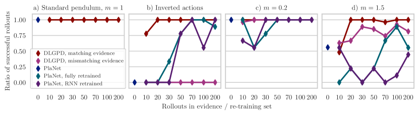
Figure 4: In addition to the cumulative rewards collected for pendulum swingup rollouts with our DLGPD model and PlaNet (see section 3.3) we also evaluated the ratio of successful control rollouts for several environment modifications and evidence (DLGPD) / re-training (PlaNet) subset sizes. As there is no common definition of ”success” for the Pendulum-v0 environment of OpenAI Gym, we defined a rollout to be successful if the last 25 planning steps of 150 total steps exceed a reward of $-1$ ($0$ is the maximum achievable reward for this environment). The experimental setting is otherwise analogous to the evaluation in section 3. We observe that DLGPD matches or outperforms the success rate of PlaNet for evidence sizes $\geq$ 20 in all settings and is able to adapt to changes in the environment (fig. 4 (b-d)) with only a few extra rollouts.

Appendix D Encoder and decoder architecture

For mapping from observation space to latent space and vice versa, we use (transposed) convolutional neural networks with ReLU non-linearities. The network architecture is similar to the encoder and decoder used in (Hafner et al., 2019). The encoder parametrizes a normal distribution by its mean $\mu$ and standard deviation $\sigma$.

Table 1: Encoder architecture

Input: 2 channel-wise concatenated RGB images (6x64x64)
Conv2D (32 filters, kernel size 4x4, stride 2) + ReLU
Conv2D (64 filters, kernel size 4x4, stride 2) + ReLU
Conv2D (128 filters, kernel size 4x4, stride 2) + ReLU
Conv2D (256 filters, kernel size 4x4, stride 2) + ReLU
$\mu$: Linear (1024 $\rightarrow$ 3), $\sigma$: Softplus(Linear(1024 $\rightarrow$ 3) + 0.55) + 0.01

Table 2: Decoder architecture

Input: 3-dimensional latent variable
Linear(3 $\rightarrow$ 1024) + ReLU
ConvTranspose2D (128 output channels, kernel size 5x5, stride 2) + ReLU
ConvTranspose2D (64 output channels, kernel size 5x5, stride 2) + ReLU
ConvTranspose2D (32 output channels, kernel size 6x6, stride 2) + ReLU
ConvTranspose2D (6 output channels, kernel size 6x6, stride 2) + Sigmoid
Output: 2 channel-wise concatenated RGB images (6x64x64)

plainnat references

References

- Al-Shedivat et al. (2018) Maruan Al-Shedivat, Trapit Bansal, Yuri Burda, Ilya Sutskever, Igor Mordatch, and Pieter Abbeel. Continuous adaptation via meta-learning in nonstationary and competitive environments. In International Conference on Learning Representations (ICLR), 2018.
- Banijamali et al. (2018) Ershad Banijamali, Rui Shu, Mohammad Ghavamzadeh, Hung Hai Bui, and Ali Ghodsi. Robust locally-linear controllable embedding. In International Conference on Artificial Intelligence and Statistics, AISTATS 2018, pages 1751–1759, 2018.
- Brockman et al. (2016) Greg Brockman, Vicki Cheung, Ludwig Pettersson, Jonas Schneider, John Schulman, Jie Tang, and Wojciech Zaremba. Openai gym, 2016.
- de Boer et al. (2005) Pieter-Tjerk de Boer, Dirk P. Kroese, Shie Mannor, and Reuven Y. Rubinstein. A tutorial on the cross-entropy method. Annals OR, 134(1):19–67, 2005.
- Deisenroth and Rasmussen (2011) Marc Peter Deisenroth and Carl Edward Rasmussen. PILCO: A model-based and data-efficient approach to policy search. In Proceedings of the 28th International Conference on Machine Learning, ICML 2011, pages 465–472, 2011.
- Deisenroth et al. (2009) Marc Peter Deisenroth, Carl Edward Rasmussen, and Jan Peters. Gaussian process dynamic programming. Neurocomputing, 72(7-9), 2009.
- Fraccaro et al. (2017) Marco Fraccaro, Simon Kamronn, Ulrich Paquet, and Ole Winther. A disentangled recognition and nonlinear dynamics model for unsupervised learning. In Advances in Neural Information Processing Systems 30: Annual Conference on Neural Information Processing Systems 2017, pages 3601–3610, 2017.
- Gal et al. (2016) Yarin Gal, Rowan McAllister, and Carl E. Rasmussen. Improving PILCO with Bayesian neural network dynamics models. In Data-Efficient Machine Learning workshop, ICML, April 2016.
- Garcia et al. (1989) Carlos E. Garcia, David M. Prett, and Manfred Morari. Model predictive control: Theory and practice - A survey. Automatica, 25(3):335–348, 1989.
- Gardner et al. (2018) Jacob R. Gardner, Geoff Pleiss, David Bindel, Kilian Q. Weinberger, and Andrew Gordon Wilson. Gpytorch: Blackbox matrix-matrix gaussian process inference with gpu acceleration. In Proceedings of the 32Nd International Conference on Neural Information Processing Systems, NIPS’18, pages 7587–7597, USA, 2018. Curran Associates Inc. URL http://dl.acm.org/citation.cfm?id=3327757.3327857.
- Gu et al. (2017) Shixiang Gu, Ethan Holly, Timothy P. Lillicrap, and Sergey Levine. Deep reinforcement learning for robotic manipulation with asynchronous off-policy updates. In 2017 IEEE International Conference on Robotics and Automation, ICRA 2017, pages 3389–3396, 2017.
- Hafner et al. (2019) Danijar Hafner, Timothy P. Lillicrap, Ian Fischer, Ruben Villegas, David Ha, Honglak Lee, and James Davidson. Learning latent dynamics for planning from pixels. In Proceedings of the 36th International Conference on Machine Learning, ICML 2019, pages 2555–2565, 2019.
- Hayashi et al. (2019) Kohei Hayashi, Masaaki Imaizumi, and Yuichi Yoshida. On random subsampling of gaussian process regression: A graphon-based analysis. CoRR, abs/1901.09541, 2019. URL http://arxiv.org/abs/1901.09541.
- II et al. (2014) Alvin Grissom II, He He, Jordan L. Boyd-Graber, John Morgan, and Hal Daumé III. Don’t until the final verb wait: Reinforcement learning for simultaneous machine translation. In Proceedings of the 2014 Conference on Empirical Methods in Natural Language Processing, EMNLP 2014, pages 1342–1352, 2014.
- Karl et al. (2017) Maximilian Karl, Maximilian Sölch, Justin Bayer, and Patrick van der Smagt. Deep variational bayes filters: Unsupervised learning of state space models from raw data. In 5th International Conference on Learning Representations, ICLR 2017, 2017.
- Killian et al. (2017) Taylor Killian, Samuel Daulton, George Konidaris, and Finale Doshi-Velez. Robust and efficient transfer learning with hidden-parameter markov decision processes. In Neural Information Processing Systems (NeurIPS), 2017.
- Kingma and Ba (2014) Diederik P. Kingma and Jimmy Ba. Adam: A Method for Stochastic Optimization. arXiv e-prints, art. arXiv:1412.6980, Dec 2014.
- Kingma and Welling (2014) Diederik P. Kingma and Max Welling. Auto-encoding variational bayes. In International Conference on Learning Representations, ICLR 2014, 2014.
- Ko et al. (2007) Jonathan Ko, Daniel J. Klein, Dieter Fox, and Dirk Hähnel. Gaussian processes and reinforcement learning for identification and control of an autonomous blimp. In 2007 IEEE International Conference on Robotics and Automation, ICRA 2007, 2007.
- Lesort et al. (2018) Timothée Lesort, Natalia Díaz Rodríguez, Jean-François Goudou, and David Filliat. State representation learning for control: An overview. Neural Networks, 108:379–392, 2018.
- Lillicrap et al. (2016) Timothy P. Lillicrap, Jonathan J. Hunt, Alexander Pritzel, Nicolas Heess, Tom Erez, Yuval Tassa, David Silver, and Daan Wierstra. Continuous control with deep reinforcement learning. In 4th International Conference on Learning Representations, ICLR 2016, 2016.
- Liu et al. (2018) Haitao Liu, Yew-Soon Ong, Xiaobo Shen, and Jianfei Cai. When gaussian process meets big data: a review of scalable gps. CoRR, 2018. URL http://arxiv.org/abs/1807.01065v2.
- Mnih et al. (2015) Volodymyr Mnih, Koray Kavukcuoglu, David Silver, Andrei A. Rusu, Joel Veness, Marc G. Bellemare, Alex Graves, Martin A. Riedmiller, Andreas Fidjeland, Georg Ostrovski, Stig Petersen, Charles Beattie, Amir Sadik, Ioannis Antonoglou, Helen King, Dharshan Kumaran, Daan Wierstra, Shane Legg, and Demis Hassabis. Human-level control through deep reinforcement learning. Nature, 518(7540):529–533, 2015.
- Oh et al. (2016) Junhyuk Oh, Valliappa Chockalingam, Satinder P. Singh, and Honglak Lee. Control of memory, active perception, and action in minecraft. In Proceedings of the 33nd International Conference on Machine Learning, ICML 2016, pages 2790–2799, 2016.
- Paszke et al. (2019) Adam Paszke, Sam Gross, Francisco Massa, Adam Lerer, James Bradbury, Gregory Chanan, Trevor Killeen, Zeming Lin, Natalia Gimelshein, Luca Antiga, Alban Desmaison, Andreas Kopf, Edward Yang, Zachary DeVito, Martin Raison, Alykhan Tejani, Sasank Chilamkurthy, Benoit Steiner, Lu Fang, Junjie Bai, and Soumith Chintala. Pytorch: An imperative style, high-performance deep learning library. In H. Wallach, H. Larochelle, A. Beygelzimer, F. d’ Alché-Buc, E. Fox, and R. Garnett, editors, Advances in Neural Information Processing Systems 32, pages 8024–8035. Curran Associates, Inc., 2019.
- Rasmussen and Kuss (2003) Carl Edward Rasmussen and Malte Kuss. Gaussian processes in reinforcement learning. In Advances in Neural Information Processing Systems 16 [Neural Information Processing Systems, NIPS 2003, pages 751–758, 2003.
- Rasmussen and Williams (2006) Carl Edward Rasmussen and Christopher K. I. Williams. Gaussian processes for machine learning. Adaptive computation and machine learning. MIT Press, 2006.
- Rezende et al. (2014) Danilo Jimenez Rezende, Shakir Mohamed, and Daan Wierstra. Stochastic backpropagation and approximate inference in deep generative models. In International Conference on Machine Learning, ICML 2014, pages 1278–1286, 2014.
- Rubinstein (1996) Reuven Y. Rubinstein. Optimization of computer simulation models with rare events. European Journal of Operations Research, 99:89–112, 1996.
- Saemundsson et al. (2018) Steindór Saemundsson, Katja Hofmann, and Marc Peter Deisenroth. Meta reinforcement learning with latent variable gaussian processes. In Conference on Uncertainty in Artificial Intelligence (UAI), 2018.
- Wang et al. (2005) Jack M. Wang, David J. Fleet, and Aaron Hertzmann. Gaussian process dynamical models. In Advances in Neural Information Processing Systems 18 [Neural Information Processing Systems, NIPS 2005, 2005.
- Watter et al. (2015) Manuel Watter, Jost Tobias Springenberg, Joschka Boedecker, and Martin A. Riedmiller. Embed to control: A locally linear latent dynamics model for control from raw images. In Advances in Neural Information Processing Systems, pages 2746–2754, 2015.
- Zhang et al. (2019) Marvin Zhang, Sharad Vikram, Laura Smith, Pieter Abbeel, Matthew J. Johnson, and Sergey Levine. SOLAR: deep structured representations for model-based reinforcement learning. In Proceedings of the 36th International Conference on Machine Learning, ICML 2019, pages 7444–7453, 2019.