A hybrid post-Newtonian – effective-one-body scheme for spin-precessing compact-binary waveforms up to merger

Abstract

We introduce TEOBResumSP: an efficient yet accurate hybrid scheme for generating gravitational waveforms from spin-precessing compact binaries. The precessing waveforms are generated via the established technique of Euler rotating aligned-spin (non-precessing) waveforms from a precessing frame to an inertial frame. We employ the effective-one-body approximant TEOBResumS to generate the aligned-spin waveforms. We obtain the Euler angles by solving the post-Newtonian precession equations expanded to (next-to)⁴ leading (second post-Newtonian) order. Current version of TEOBResumSP produces precessing waveforms through the inspiral phase up to the onset of the merger. We compare TEOBResumSP to current state-of-the-art precessing approximants NRSur7dq4, SEOBNRv4PHM, and IMRPhenomPv3HM in terms of frequency-domain matches of the $\ell=2$ gravitational-wave strain for 200 cases of precessing compact binary inspirals with orbital inclinations up to 90 degrees, mass ratios up to four, and the effective precession parameter $\chi_{p}$ up to 0.75. We further provide an extended comparison with SEOBNRv4PHM involving 1030 more inspirals with $\chi_{p}$ ranging up to one and mass ratios up to 10. We find that 91% of the TEOBResumSP-NRSur7dq4 matches, 85% of the TEOBResumSP-SEOBNRv4PHM matches, and 77% of the TEOBResumSP-IMRPhenomPv3HM matches are greater than $0.965$. Most of the significant disagreements occur for large mass ratios and $\chi_{p}\gtrsim 0.6$. We identify the mismatch of the non-precessing $(2,1)$ mode as one of the leading causes of disagreements. We also introduce a new parameter, $\chi_{\perp,\text{max}}$, to measure the strength of precession and hint that the strain mismatch between the above waveform approximants shows an exponential dependence on $\chi_{\perp,\text{max}}$ though this requires further study. Our results indicate that TEOBResumSP is on its way to becoming a robust precessing approximant to be employed in the parameter estimation of generic-spin compact binaries.

I Introduction

Gravitational-wave events have become routine in observational astronomy: the Advanced LIGO Aasi et al. (2015)-Virgo Acernese et al. (2015) interferometers detected at least ten binary black hole coalescences and one binary neutron star merger during the first and second observing runs Abbott et al. (2016a, 2017a, b, 2017b, 2017c, 2017d, 2019a); Venumadhav et al. (2019, 2020); Nitz et al. (2019, 2020). The third observing run began on 1 April 2019 and delivered by its [premature] end a year later the second binary neutron star merger Abbott et al. (2020a), two binary black hole mergers with significant mass asymmetry Abbott et al. (2020b, c), the second possibly involving the most massive neutron star discovered yet, another black hole merger leading to the formation of an intermediate mass black hole Abbott et al. (2020d), and additionally more than four dozen triggers with false alarm rates of less than one per year gra . A significant fraction of these triggers turned out to be genuine gravitational-wave events caused by the inspiral and merger of stellar mass compact objects Abbott et al. (2020e).

The properties of the compact objects such as masses and spins can be obtained via parameter estimation studies that are conducted on a sufficiently “cleaned” version of the relevant segment of the detector data. This requires a large set of “realistic” theoretical gravitational waveform templates which can be cross-correlated with the data. For stellar-mass compact binary systems, there are four main approaches to generating the theoretical gravitational waves (GWs) resulting from compact binary inspirals: post-Newtonian theory Blanchet (2014), numerical relativity Gourgoulhon (2012); Centrella et al. (2010), effective-one-body theory Buonanno and Damour (1999, 2000), and phenomenological template construction Ajith et al. (2007, 2008). More recently, there has also been an emergence of surrogate methods which we discuss below.

Post-Newtonian (PN) theory employs a large-separation (weak-field) expansion to the Einstein field equations. Current PN technology for the evolution of quasi-circular inspirals is at the 3.5PN level with partial higher-order PN information available Bernard et al. (2018); Messina et al. (2019). As PN information is fully analytical, the resulting waveforms can be evaluated very quickly. Consequently, the LIGO-Virgo Collaboration (LVC) has at its disposal a plethora of PN-based Taylor waveform approximants summarized in Ref. Buonanno et al. (2009). As PN theory is valid in the weak-field, adiabatic regime, these approximants are appropriate for modelling only the inspiral phase and extracting the chirp mass Damour et al. (2012); Abbott et al. (2020a), with possibly PhenSpinTaylorRD Sturani et al. (2010) as an exception, which is a hybrid model that matches spinning PN inspiral waveforms and fits to NR ringdown waveforms.

Binary black hole (BBH) systems are more massive, thus transit through the LIGO-Virgo detection bandwidth much more quickly than binary neutron stars (BNSs), e.g., GW150914 lasted less than 20 milliseconds Abbott et al. (2016a) whereas GW170817 lasted nearly a minute Abbott et al. (2017a). As such, we can detect only the last few dozen cycles of their GWs before merger. Such GWs are generated in the very-strong-gravity regime where PN approximation is not reliable. This is the domain of numerical relativity (NR). Since the breakthroughs of 2005 Pretorius (2005); Campanelli et al. (2006); Baker et al. (2006), it has become routine to evolve strongly gravitating spacetimes of compact binary mergers on large computing clusters. There are now several NR catalogs containing thousands of simulations of compact binary inspirals Mroue et al. (2013); Boyle et al. (2019); SXS ; Jani et al. (2016); GA_ ; RIT ; Healy et al. (2017); Dietrich et al. (2018); CoR . Of these, the most comprehensive is the 2019 SXS catalog which contains 2018 simulations of precessing systems with the dimensionless Kerr spin parameter up to 0.998 Boyle et al. (2019).

As the number of NR simulations increased, it became possible to build hybrid (phenomenological) waveform models by matching PN inspiral waveforms and fits to NR waveforms. The initial model, PhenomA Ajith et al. (2007, 2008), combined the TaylorT1 PN waveform model with a two-dimensional fit to a set of non-precessing NR simulations. The model was steadily improved through versions B Ajith et al. (2011), C Santamaria et al. (2010), and D Husa et al. (2016); Khan et al. (2016). Specific models were then developed for binary neutron stars (PhenomD_NRTidal Dietrich et al. (2017, 2019a)), higher modes (PhenomHM London et al. (2018)), and spin precession (PhenomP Hannam et al. (2014); Schmidt et al. (2015)). Subsequently, the non-precessing models have gone through several upgrades Pratten et al. (2020a); García-Quirós et al. (2020a, b), just as the precessing ones have Chatziioannou et al. (2017); Khan et al. (2019a, b); Pratten et al. (2020b); Estellés et al. (2020) with IMRPhenomPv3HM Khan et al. (2019b) being employed in the analysis of the most recent GW events. Note that the recent IMRPhenomX family match a mix of EOB, PN waveforms with NR Pratten et al. (2020a); García-Quirós et al. (2020a); Pratten et al. (2020b). Phenom models generate frequency-domain waveforms with the corresponding time-domain waveforms obtained by inverse fast Fourier transforms, only exception being IMRPhenomTP Estellés et al. (2020) which is a direct time-domain construction. Since GW data analysis is performed in the frequency-domain and as Phenom waveforms are fast to generate, the Phenom family has become one of the most commonly used set of waveform approximants in the parameter estimation of GW events as well as in other areas of GW science where fast, reliable waveforms are required.

The effective-one-body (EOB) approach bridges PN theory and NR. It maps the two-body PN motion to a geodesic motion in an effective spacetime via a deformation performed in terms of the symmetric mass ratio Buonanno and Damour (1999, 2000). In its core, EOB contains an effective Hamiltonian for aligned-spin systems, which resums the PN series in a suitable way to better capture the effects of the strong-field regime Damour and Nagar (2009). The inspiral is driven by a specially factorized/resummed radiation-reaction force Damour and Nagar (2014a). The resulting multipolar gravitational waveforms are also written in a factorized form Damour et al. (2009); Pan et al. (2011). The analytical EOB model is further supplemented with input from non-precessing NR simulations, thus extending the EOB evolution through the merger and, if it exists, ringdown stages. These so-called EOBNR models Damour and Nagar (2014b); Bohé et al. (2017); Nagar et al. (2017) have been incorporated into several waveform approximants Pürrer (2014); Babak et al. (2017); Cotesta et al. (2018); Dietrich et al. (2019a); Nagar et al. (2018) that are used for parameter estimation studies of LIGO-Virgo GW events. The main advantages of employing EOB-based waveform approximants for parameter estimation are that they (i) push the validity of the model beyond the PN weak-field regime (ii) can be extended to the full parameter space, and (iii) are much faster to evolve than NR simulations. EOB models can also accurately model binary neutron star coalescences from low frequencies and up to merger Damour and Nagar (2010); Damour et al. (2012); Bernuzzi et al. (2012); Lackey et al. (2014); Bernuzzi et al. (2015); Hinderer et al. (2016); Steinhoff et al. (2016); Dietrich et al. (2019b); Akcay et al. (2019); Lackey et al. (2019); Matas et al. (2020), thus offering a viable alternative to PhenomTidal models Husa et al. (2016); Khan et al. (2016); Dietrich et al. (2019a); Thompson et al. (2020), or to PN-based tidal models (e.g., TaylorF2 with tides up to 7.5PN order Damour et al. (2012); Vines et al. (2011); Henry et al. (2020)) In short, EOB can provide NR-PN-faithful waveforms for parameter estimation studies of both long and short inspiral-merger-ringdown signals, and for extracting information about tides.

Although it has thus far been very difficult to distinguish the effects of precession on the gravitational waves from the few dozen sources hitherto detected, there are at least four GW events for which it has been inferred that the pre-merger binary components have nonzero spin. These are GW151226 Abbott et al. (2016b), where at least one black hole has dimensionless spin $>0.28$ Abbott et al. (2019b), GW170729 Abbott et al. (2019a); Chatziioannou et al. (2019), where at least one black hole has dimensionless spin $>0.27$ Abbott et al. (2019b), GW190412 where either the primary Abbott et al. (2020b) or the secondary Mandel and Fragos (2020) has positive dimensionless spin depending on the priors used, and GW190521 with both black holes having dimensionless spins $>0.5$ Abbott et al. (2020d, f). There are two additional events, GW170121 and GW170403, that seem to have at least one anti-aligned spinning component Venumadhav et al. (2020).

In binaries containing spinning black holes and/or millisecond pulsars, the spin-orbit and the spin-spin interactions contribute significantly to the phase and modulate distinguishably the amplitude of the emitted GWs. For example, there are more than 20 precession cycles contributing to the phasing of the GWs for a BNS with total mass of 3 $M_{\odot}$ inspiralling from 30 Hz Apostolatos et al. (1994). Therefore, given that the required relative phase errors of the theoretical waveform templates must be $\lesssim 5\times 10^{-4}$ to avoid waveform systematics with Advanced LIGO-Virgo design sensitivity Pürrer and Haster (2020), the templates must incorporate the effects of precession. Neglecting precession for high-mass ratio binaries can cause event rate losses of $\sim 15\%$ and as high as 25% - 60% for the worst cases Harry et al. (2016); Calderón Bustillo et al. (2017). For the third generation detectors such as the Einstein Telescope and Cosmic Explorer, these errors will need to be $\lesssim 10^{-6}$ which will be a tremendous challenge as the EOB, PN, and Phenom template families will need to be improved by three orders of magnitude while NR errors will need to be reduced by at least an order of magnitude Pürrer and Haster (2020).

There has been a dedicated and an ever-increasing effort to produce accurate gravitational waveforms from precessing compact binary systems. Initial developments were made in post-Newtonian theory Barker and O’Connell (1979); Thorne and Hartle (1984) after the pioneering work of Mathisson, Papapetrou, and Dixon (MPD) on the motion of spinning test particles in curved spacetimes Mathisson (1937); Papapetrou (1951); Dixon (1970). There are now several waveform approximants available for precessing spin analysis (and implemented in the LIGO Algorithm Library (LAL) LIGO Scientific Collaboration (2018)), which are: (i) $\mathtt{SpinTaylorT}$class of approximants which employ 1.5PN analytical expressions of Ref. Arun et al. (2009) for the waveform harmonic modes as functions of the spherical angles of the Newtonian orbital angular momentum vector. (ii) $\mathtt{IMRPhenomP}$class of approximants which transform non-precessing Phenom waveforms into precessing ones using Euler rotations for which the angles are obtained from the PN spin precession equations Hannam et al. (2014); Schmidt et al. (2015); Khan et al. (2019a, b); Pratten et al. (2020b); Estellés et al. (2020). In particular, Ref. Hannam et al. (2014) showed that “the essential phenomenology of the seven-dimensional parameter space of binary configurations” can be modeled using just three parameters. (iii) $\mathtt{SEOBNR}$class of approximants Pan et al. (2014a); Babak et al. (2017); Ossokine et al. (2020) which evolve the EOB dynamics and precession equations as a coupled system to determine the Euler angles for the rotation of the non-precessing waveform modes. (iv) NRSurclass which are surrogate waveform models in which the surrogate is trained using large sets of precessing NR waveforms that are Euler-rotated to a certain non-inertial co-orbital frame. With the exception of the NRSur family, the above-listed approximants solve the same precession equations, albeit truncated at different PN orders or suitably incorporated into a particular EOB Hamiltonian. The solutions to the precession equations are then translated into the spherical angles of the Newtonian orbital angular momentum. The precessing waveforms are constructed either via the analytical 1.5 PN expressions of Ref. Arun et al. (2009) (only for the SpinTaylorT family) or by using the so-called twist method of Ref. Schmidt et al. (2011) which is what concerns us in this article so we provide some details next.

The seeds of the twist method were sown in Ref. Apostolatos et al. (1994), where it was identified that the waveform phase can be decomposed into a non-modulating main carrier phase and a modulation term due to precession. Ref. Buonanno et al. (2003) used this decomposition to construct waveform templates with the unmodulated carrier phase given by nonspinning frequency domain fits to the full 2 PN phase. It was later shown in Refs. Schmidt et al. (2011, 2012) that the correct unmodulated carrier phase is given by the non-precessing, but spinning phase. Ref. Buonanno et al. (2003) also introduced a special non-inertial frame, called the precessing frame, in which the orbital phase agreed with the PN orbital phase of a non-spinning system. In other words, the modulations in the gravitational waveform phase due to precession factored out. Subsequently, Ref. Gualtieri et al. (2008) obtained rigorous expressions for the transformation of waveform multipoles under rotations, which were then employed by Ref. Campanelli et al. (2009) in order to generate precessing post-Newtonian waveforms to compare with their numerical results.

A crucial step toward obtaining full (inspiral-merger-ringdown) precessing waveforms was taken by Ref. Schmidt et al. (2011) which employed a time-dependent frame rotation of the harmonic modes of the Weyl scalar $\Psi_{4}$ into the “quadrupole-aligned” (QA) frame defined by the direction toward which the amplitudes of the $(2,\pm 2)$ modes are maximized, which turned out to coincide with the instantaneous direction of the total orbital angular momentum vector. Ref. Schmidt et al. (2012) used this frame rotation on the $\ell=2$ modes of the gravitational waveform and demonstrated that the model is better than 99% accurate. Ref. O’Shaughnessy et al. (2011) introduced a frame similar to the QA frame by equating the radiation axis with the eigenvector of the rotation group generators which had the largest absolute eigenvalue. Subsequently, Ref. Boyle et al. (2011) demonstrated that the special frames of Refs. Schmidt et al. (2011, 2012) and Ref. O’Shaughnessy et al. (2011) are the same if one includes only the $(2,\pm 2)$ modes in the $m$-mode sum. Additionally, Ref. Boyle et al. (2011) rigorously showed the necessity for a third Euler angle $\gamma$ in order to obtain a unique precessing frame which they dubbed the minimal-rotation frame.

The size of the parameter space for generic precessing binaries presents another formidable challenge for parameter estimation as the number of intrinsic parameters increases from three (mass ratio and two spin magnitudes) for configurations where the spins are (anti)parallel to the orbital angular momentum, which we refer to as either non-precessing or aligned-spin configurations, to seven for binary black holes, and even more in the case of binary neutron stars to additionally parametrize their tidal interactions. As brute-force coverage of such a large space is computationally expensive, approaches aimed at reducing the computational burden without compromising waveform accuracy have emerged. Of particular importance is Ref. Schmidt et al. (2012) which used an effective parametrization reducing the number of parameters to two in the QA frame by introducing an effective spin parameter​​ ​​  $\chi_{\text{eff}}$. The precessing waveform is then obtained by twisting the QA waveform with three Euler angles as already described. Ref. Schmidt et al. (2015) took this approach further by packaging the four in-plane (perpendicular to the Newtonian angular momentum) components of the binary’s spin vectors into a single effective precession parameter, $\chi_{p}$, thereby reducing the dimensionality of the parameter space to four. On a parallel front, methods based on reduced-basis/order modelling were developed for generating fast, non-precessing waveforms Field et al. (2011); Herrmann et al. (2012); Canizares et al. (2013); Pürrer (2014); Canizares et al. (2015); Pürrer (2014, 2016); Bohé et al. (2017); Doctor et al. (2017); Cotesta et al. (2018); Dietrich et al. (2019a); Cotesta et al. (2020); Matas et al. (2020). And finally, NR-“trained” precessing waveform surrogates Blackman et al. (2014, 2017); Varma et al. (2019); Williams et al. (2019) have emerged as the number of precessing NR simulations increased SXS . Other approaches are also being developed such as “the two-harmonic approximation” Fairhurst et al. (2019).

In summary, there now exist several diverse precessing waveform approximants of which the most prominent ones are NRSur7dq4 Varma et al. (2019), $\mathtt{IMRPhenomPv3HM}$ Khan et al. (2019b) (previously PhenomPv2), and SEOBNRv4PHM Ossokine et al. (2020) (previously $\mathtt{SEOBNRv3}$). These three approximants (along with the more recent IMRPhenomXPHM Pratten et al. (2020b)) have quickly become the preferred waveform models for parameter estimation by the LVC. However, they do not agree perfectly, which can lead to biases as was illustrated, e.g., by Ref. Williamson et al. (2017) via an SEOBNRv3-IMRPhenomPv2 comparison, highlighting what one should always keep in mind: waveform approximants are approximate as the name implies so they can disagree, therefore it is beneficial to have several approximants.

This paper is the first of a series that develops TEOBResumSP, a generic-spin approximant based on the Euler rotation of aligned-spin waveforms generated by TEOBResumS  Nagar et al. (2018). TEOBResumS is a state-of-the-art aligned-spin EOBNR model with enhanced spin-orbit, spin-spin, and tidal interactions Nagar et al. (2019a); Akcay et al. (2019) that is very fast Nagar and Rettegno (2019) and robustly produces inspiral-merger-ringdown waveforms for five additional modes beside the dominant (2,2) mode Nagar et al. (2019b, 2020). TEOBResumS is very different in its design from SEOBNRv4PHM, in particular in the spin sector Rettegno et al. (2019), thus provides the only fully independent waveform model from the approximants currently in use for GW analysis (e.g., PhenomPv3 uses fits of SEOBNR waveforms Ossokine et al. (2020)). Our goal in this initial implementation of TEOBResumSP is to introduce minimal modifications to the existing TEOBResumS infrastructure. Therefore, we opt for an approach whereby we produce aligned, constant spin waveforms using TEOBResumS then generate inspiral-merger precessing waveforms by twisting the non-precessing waveforms as is done in the IMRPhenomP, SEOBNR, and NRSur families. We delegate the attachment of the ringdown portion of the precessing waveforms to the next version of TEOBResumSP.

This article is organized as follows. We start by introducing the PN precession equations in Sec. II. In Sec. III, we present details for the waveform twist operation. In Sec. IV, we compare TEOBResumSP waveforms with the following waveform approximants: NRSur7dq4, IMRPhenomPv3HM, and SEOBNRv4PHM. We summarize our results in Sec. V. We work in geometrized units setting $G=c=1$ from which one can recover the SI units via $GM_{\odot}/c^{3}\approx 4.925491\times 10^{-6}\,$sec, where $M_{\odot}$ denotes a solar mass. We use bold font to denote Euclidean three-vectors with an overhat representing three-vectors of unit length. Overdots denote derivatives with respect to time.

II An Overview of Precessing Compact Binary Systems

Let us consider a compact binary system in a quasi-spherical inspiral with the subscript 1 labelling the primary and 2 labelling the secondary component. Accordingly, the individual masses are denoted by $m_{1}$ and $m_{2}$ with $m_{1}\geq m_{2}$. The total mass is defined as $M=m_{1}+m_{2}$. Let us also introduce the mass ratio $q\equiv m_{2}/m_{1}\leq 1$, the reduced mass $\mu\equiv Mq/(1+q)^{2}$, and the symmetric mass ratio $\eta\equiv q/(1+q)^{2}$. Note that in this article, we often set $M=1$, e.g., Eqs. (1a)-(1c), but sometimes restore solar-mass units ($M_{\odot}$) for $M$, cf. Eqs. (11), (14). We additionally endow the binary components with spins $\mathbf{S}_{1},\mathbf{S}_{2}$, respectively, where $\mathbf{S}_{i}\equiv m_{i}^{2}\bm{\chi}_{i}$ with $|\bm{\chi}_{i}|\leq 1$ for $i=1,2$.

II.1 Spin-orbit precession equations

The Newtonian orbital angular momentum for the binary is given by $\mathbf{L}_{\text{N}}={\mu}\,\mathbf{r}\times\mathbf{v}$, where $\mathbf{r},\mathbf{v}$ are the relative separation and velocity vectors of the binary in the usual center-of-mass frame. Note that $\mathbf{L}_{\text{N}}$ is different from its non-Newtonian counterpart $\mathbf{L}=\mathbf{r}\times\mathbf{p}$, where $\mathbf{p}$ is the relative momentum. This distinction, due to $\mu\mathbf{v}\neq\mathbf{p}$, is a consequence of the fully general relativistic MPD equations for the motion of a spinning test mass in curved spacetime. From PN theory, one obtains $\mathbf{L}=\mathbf{L}_{\text{N}}+\Delta\mathbf{L}_{\text{1PN}}+\ldots$ with correction terms, $\Delta\mathbf{L}_{n\text{PN}}$, known up to 3.5PN (see, e.g., Eq. (4.7) of Ref. Bohe et al. (2013)). Note that, by definition, the Newtonian $\mathbf{L}_{\text{N}}$ remains perpendicular to the orbital plane.

Let $\omega$ be the orbital frequency. Then, via Kepler’s third law: $r\equiv|\mathbf{r}|=\omega^{-2/3}$. Accordingly, $\text{L}_{\text{N}}\equiv|\mathbf{L}_{\text{N}}|=\mu r^{2}\omega=m_{1}m_{2}/\omega^{1/3}=\eta/v$, where we have introduced $v\equiv|\mathbf{v}|=\omega^{1/3}$, i.e., the relative speed between the binary’s components in the usual center-of-mass frame. Clearly, $v<1$ and furthermore, $v\ll 1$ for most of the inspiral (recall, $v=v/c$ in restored units). Note that each power of $v$ corresponds to a half PN order. In this work, we use $v$ to track the orders in the precession equations. Consequently, we reserve expressions such as next-to-leading order (NLO) to verbally track each power of $v$ beyond a given leading-order (LO) expression.

One can start with the general MPD equations of motion and obtain the PN expansions for the time evolution of $\mathbf{S}_{1},\mathbf{S}_{2}$. The details of this derivation can be found in, e.g., Secs.  II, III of Ref. Bohé et al. (2015), and Sec. II of Ref. Racine et al. (2009). Up to NLO, i.e., 0.5PN, the orbital angular momentum and spin precession equations are given by Apostolatos et al. (1994); Kidder (1995)

$$\dot{\mathbf{S}}_{1}^{\text{NLO}} =v^{5}\,\eta\left(2+\frac{3}{2}q\right)\left(\!\hat{\,\mathbf{L}}_{\text{N}}\times\mathbf{S}_{1}\right)$$ (1a)

$$+\frac{v^{6}}{2}\left\{\mathbf{S}_{2}-3[(q\mathbf{S}_{1}+\mathbf{S}_{2})\cdot\!\hat{\,\mathbf{L}}_{\text{N}}]\,\!\hat{\,\mathbf{L}}_{\text{N}}\right\}\times\mathbf{S}_{1},$$

$$\dot{\mathbf{S}}_{2}^{\text{NLO}} =v^{5}\,\eta\left(2+\frac{3}{2q}\right)\left(\!\hat{\,\mathbf{L}}_{\text{N}}\times\mathbf{S}_{2}\right)$$ (1b)

$$+\frac{v^{6}}{2}\left\{\mathbf{S}_{1}-3[(\mathbf{S}_{1}+q^{-1}\mathbf{S}_{2})\cdot\!\hat{\,\mathbf{L}}_{\text{N}}]\,\!\hat{\,\mathbf{L}}_{\text{N}}\right\}\times\mathbf{S}_{2},$$

$$\dot{\hat{\,\mathbf{L}}}_{\text{N}}^{\text{NLO}} =-\frac{v}{\eta}\left(\dot{\mathbf{S}}_{1}^{\text{NLO}}+\dot{\mathbf{S}}_{2}^{\text{NLO}}\right).$$ (1c)

Note that, as is usual in the literature, we present the orbit-averaged evolution equations. As such, our solutions to these equations do not capture the nutation of $\mathbf{L}_{\text{N}}$, but this is of no consequence for parameter estimation purposes at the sensitivity of the advanced GW detectors Pan et al. (2014b). For non-averaged versions, cf. App. A of Ref. Bohé et al. (2015).

The particular form of Eq. (1c) above is the result of total angular momentum conservation: $\dot{\mathbf{J}}=0$, where $\mathbf{J}=\mathbf{L}+\mathbf{S}$ with $\mathbf{S}\equiv\mathbf{S}_{1}+\mathbf{S}_{2}$. The forms of Eqs. (1a-1c) have the added benefit that the evolution of the Newtonian orbital angular momentum can be written as a classical mechanical precession equation:

$$\dot{\hat{\,\mathbf{L}}}_{\text{N}}^{\text{NLO}}=\bm{\Omega}_{\text{NLO}}\times\!\hat{\,\mathbf{L}}_{\text{N}},$$ (2)

where $\bm{\Omega}_{\text{NLO}}$ can be extracted straightforwardly from Eqs. (1a - 1c).

The effect of radiation reaction is implicit in $v=v(t)$ in Eqs. (1a-1c). For nonspinning systems, $\dot{v}=\dot{v}(v)$ is fully known as a PN series starting from $\sim v^{9}$ and going up to 3.5PN order $\sim v^{16}$. For systems with spin, spin-orbit terms enter first at 1.5PN and spin-spin terms at 2PN. Here, we employ the TaylorT4 resummed form of $\dot{v}(v)$ Buonanno et al. (2003, 2009) as adopted in the SpinTaylorT4 approximant. The series coefficients for $\dot{v}(v)$ can be found, e.g., in App. A of Ref. Chatziioannou et al. (2013).

For precessing binaries, there are three time scales of relevance: radiation-reaction timescale $T_{\text{RR}}$, precession time scale $T_{\text{pr}}$, and orbital time scale $T_{\text{orb}}$. Integrating $\dot{v}\sim v^{9}$ yields $T_{\text{RR}}\sim v^{-8}$. From $v=\omega^{1/3}$, we obtain $T_{\text{orb}}\sim v^{-3}$. Finally, the precession equation (1a) gives $T_{\text{pr}}\sim|\mathbf{S}_{1}|/|\dot{\mathbf{S}}_{1}|\sim v^{-5}$. Since $v\ll 1$ mostly, we have the following separation of timescales:

$$T_{\text{orb}}\ll T_{\text{pr}}\ll T_{\text{RR}}.$$ (3)

Thanks to this separation of scales, we expect our hybrid approach, which combines EOB dynamics with PN precession, to work well as we show in Sec. IV.

Recall that Eqs. (1a - 1c) are 0.5-PN (NLO) accurate. Though this is the usual order in the literature, we employ versions of the precession ODEs that have been pushed to the limit of the current analytical PN knowledge, which we denote as N4LO (2 PN) here. As far we can tell these have never appeared in a journal article, but exist in written form in several approximants such as SpinTaylorT4. Defining $\delta m=m_{1}-m_{2}$ in natural units [e.g., $m_{1}=1/(1+q)$], the N4LO spin-orbit precession ODEs read

$$\dot{\mathbf{S}}_{1}^{\text{N4LO}} =\ \dot{\mathbf{S}}_{1}^{\text{NNLO}}+v^{9}\left[\frac{27}{32}+\frac{3\eta}{16}-\frac{105\eta^{2}}{32}-\frac{\eta^{3}}{48}+\delta m\left(-\frac{27}{32}+\frac{39\eta}{8}-\frac{5\eta^{2}}{32}\right)\right](\!\hat{\,\mathbf{L}}_{\text{N}}\times\mathbf{S}_{1}),$$ (4a)

$$\dot{\mathbf{S}}_{2}^{\text{N4LO}} =\ \dot{\mathbf{S}}_{2}^{\text{NNLO}}+v^{9}\left[\frac{27}{32}+\frac{3\eta}{16}-\frac{105\eta^{2}}{32}-\frac{\eta^{3}}{48}-\delta m\left(-\frac{27}{32}+\frac{39\eta}{8}-\frac{5\eta^{2}}{32}\right)\right](\!\hat{\,\mathbf{L}}_{\text{N}}\times\mathbf{S}_{2}),$$ (4b)

$$\dot{\hat{\,\mathbf{L}}}_{\text{N}}^{\text{N4LO}} =\text{L}^{-1}_{2\text{PN}}\left[\frac{v}{\eta}\left(-\dot{\mathbf{S}}_{1}^{\text{N4LO}}-\dot{\mathbf{S}}_{2}^{\text{N4LO}}\right)-v^{3}\left(c_{S1}\dot{\mathbf{S}}_{1}^{\text{NNLO}}+c_{S2}\dot{\mathbf{S}}_{2}^{\text{NNLO}}\right)\right.$$ (4c)

$$\qquad\qquad\left.-v^{3}\left\{c_{S1L}\left(\left[\frac{-v}{\eta}(\dot{\mathbf{S}}_{1}^{\text{NLO}}+\dot{\mathbf{S}}_{2}^{\text{NLO}})(\!\hat{\,\mathbf{L}}_{\text{N}}\cdot\mathbf{S}_{1})\right]+\!\hat{\,\mathbf{L}}_{\text{N}}\left[-\frac{v}{\eta}\dot{\mathbf{S}}_{2}^{\text{NLO}}\cdot\mathbf{S}_{1}+\!\hat{\,\mathbf{L}}_{\text{N}}\cdot\dot{\mathbf{S}}_{1}^{\text{NNLO}}\right]\right)+(1\leftrightarrow 2)\right\}\right],$$

where

$$\dot{\mathbf{S}}_{1}^{\text{NNLO}} =\ \dot{\mathbf{S}}_{1}^{\text{NLO}}$$

$$+ v^{7}\left[\frac{9}{16}+\frac{5\eta}{4}-\frac{\eta^{2}}{24}+\delta m\left(-\frac{9}{16}+\frac{5\eta}{8}\right)\right](\!\hat{\,\mathbf{L}}_{\text{N}}\times\mathbf{S}_{1}),$$ (5a)

$$\text{L}_{2\text{PN}} =1+v^{2}\left(\frac{3}{2}+\frac{\eta}{6}\right)+v^{4}\left(\frac{27}{8}-\frac{19\eta}{8}+\frac{\eta^{2}}{24}\right),$$ (5b)

$$c_{S1} =-\frac{1}{4}\left(3+\frac{1}{m_{1}}\right),$$ (6a)

$$c_{S1L} =-\frac{1}{12}\left(1+\frac{27}{m_{1}}\right).$$ (6b)

$\dot{\mathbf{S}}_{2}^{\text{NNLO}},c_{S2},c_{S2L}$ can be obtained via the $(1\leftrightarrow 2)$ exchange.

Note that from NNLO on, one no longer has a standard precession equation for $\dot{\hat{\,\mathbf{L}}}_{\text{N}}$ of the form of Eq. (2). In fact, as can be seen from Eq. (4c), $\dot{\hat{\,\mathbf{L}}}_{\text{N}}$ has components both perpendicular and parallel to $\!\hat{\,\mathbf{L}}_{\text{N}}$. Therefore, we define Sturani

$$\dot{\hat{\,\mathbf{L}}}_{\text{N},\perp}^{\text{N4LO}}\equiv\ \dot{\hat{\,\mathbf{L}}}_{\text{N}}^{\text{N4LO}}-(\!\hat{\,\mathbf{L}}_{\text{N}}\cdot\dot{\hat{\,\mathbf{L}}}_{\text{N}}^{\text{N4LO}})\!\hat{\,\mathbf{L}}_{\text{N}},$$ (7)

which then satisfies

$$\dot{\hat{\,\mathbf{L}}}_{\text{N},\perp}^{\text{N4LO}}=\bm{\Omega}_{L}^{\text{N4LO}}\times\!\hat{\,\mathbf{L}}_{\text{N}}^{\text{N4LO}}.$$ (8)

We use the solutions of Eq. (7)​​ , to compute $\!\hat{\,\mathbf{L}}_{\text{N}}(t)$, but we have also used directly the solutions to Eq. (4c) and found relative differences in the components of $\!\hat{\,\mathbf{L}}_{\text{N}}$ of $\lesssim 10^{-4}$. We present the derivational details of these N4LO expressions in App. A.

There are indications that the PN precession equations converge with increasing PN order despite missing higher-order information Ossokine et al. (2015). Indeed, we have found it slightly more beneficial to work with the N4LO precession equations rather than the NLO versions. We illustrate this is in App. B, where we show that the N4LO-Euler-angle twisted TEOBResumSP agrees better with both NRSur7dq4 and SEOBNRv4PHM than its NLO counterpart. This agreement is demonstrated specifically in terms of waveform strain mismatches which we introduce in Sec. IV. The NLO-N4LO disagreement is more severe for systems with more mass asymmetry, i.e., smaller values of $q$, which we show in terms of Euler angles in Fig. 13 in App. A. As the figure exhibits, there is considerable Euler-angle dephasing between NLO, NNLO, and N4LO solutions for small $q$, but no such dephasing between N3LO and N4LO, which we somewhat expect since their difference is at 2 PN. We discuss the various ODE orders further in App. A We should add that instantaneous corrections to the orbit-averaged expressions start entering at N3LO Bohé et al. (2015) which we do not take into account here,

As already mentioned, it is useful to package the six spin degrees of freedom into a space of lower dimensions. This is usually done by considering the projections of $\mathbf{S}_{1},\mathbf{S}_{2}$ parallel and orthogonal to $\!\hat{\,\mathbf{L}}_{\text{N}}(t)$, resulting in two commonly employed scalar quantities. The parallel scalar is Ajith (2011); Damour (2001); Racine (2008)

$$\chi_{\text{eff}}=M^{-2}\left[(1+q)\mathbf{S}_{1}\cdot\!\hat{\,\mathbf{L}}_{\text{N}}+(1+q^{-1})\mathbf{S}_{2}\cdot\!\hat{\,\mathbf{L}}_{\text{N}}\right]$$ (9)

which is a conserved quantity of the orbit-averaged precession equations over the precession timescale Racine (2008). The orthogonal parameter is $\chi_{p}$ of Ref. Schmidt et al. (2015) defined as ​​

$$\chi_{p}\equiv\frac{m_{1}^{-2}}{\left(2+3q/2\right)}\max\left\{\!\left(2+\frac{3q}{2}\right)\!|\mathbf{S}_{1,\perp}|,\left(2+\frac{3}{2q}\right)\!|\mathbf{S}_{2,\perp}|\right\},$$ (10)

where $\mathbf{S}_{1,\perp},\mathbf{S}_{2,\perp}$ denote the components of $\mathbf{S}_{1}(t),\mathbf{S}_{2}(t)$ perpendicular to $\!\hat{\,\mathbf{L}}_{\text{N}}$, respectively. Both $\chi_{\text{eff}}$ and $\chi_{p}$ are commonly used in the LVC analysis of GW events Abbott et al. (2019a).

We now introduce a new orthogonal parameter

$$\chi_{\perp,\max} \equiv M^{-2}\max\left|\,\mathbf{S}_{1,\perp}+\mathbf{S}_{2,\perp}\right|,$$ (11)

where we take the maximum value of the norm over the entire time evolution. $\chi_{\perp,\text{max}}$ seems to encode the strength of precession as we show in Secs. IV.2-IV.4. Note that $\chi_{\perp,\text{max}}$ is bounded above by $(1+q^{2})/(1+q)^{2}$ which yields 0.5 for $q=1$ and 1 in the test-mass limit.

II.2 Reference frames

When considering precessing systems, there are two special frames of reference which have their respective $z$-axes aligned with $\mathbf{L}_{0}\equiv{\mathbf{L}}_{\text{N}}(t_{0})$ and ${\mathbf{L}}_{\text{N}}(t)$, where $t_{0}$ is some arbitrary time at the initial configuration of each binary. It is common in the waveform community to set $t=0$ to coincide with the peak of the non-precessing (2,2) mode, which then gives us $t_{0}<0$. In what follows, we assume a constant shift in $t$ such that the initial time is given by $t_{0}=0$ with the peak time positive as in done in TEOBResumS waveforms. Therefore, we write $\mathbf{L}_{0}=\mathbf{L}_{\text{N}}(0)$ and similarly for all other relevant quantities. We refer to the $\mathbf{L}_{\text{N}}(0)$ and $\mathbf{L}_{\text{N}}(t)$ frames as the $\mathbf{L}_{0}$ frame, and the co-precessing frame, respectively. Clearly, the $\mathbf{L}_{0}$ frame is inertial whereas the co-precessing frame is not. One can additionally introduce a second inertial frame, $\mathbf{J}_{0}$, where one aligns the $z$-axis with $\hat{\mathbf{J}}$ (Newtonian, 1PN or 2PN) either at the initial time or at the peak of the orbital frequency. For reasons that we explain in Sec. II.3, we choose $\mathbf{J}_{0}\equiv{\mathbf{J}}_{\text{2PN}}(0)$ obtained from the N4LO solutions for $\mathbf{L}_{\text{N}},\mathbf{S}_{1},$ and $\mathbf{S}_{2}$. Note that our $\mathbf{J}_{0}$ is different than the one introduced in Ref. Apostolatos et al. (1994), which is given by $\hat{\mathbf{J}}_{\text{N}}-\epsilon\,\hat{\mathbf{J}}_{\text{N}}\times\!\hat{\,\mathbf{L}}_{\text{N}}$, where $\epsilon\ll 1$ and the ODEs are truncated at NLO with the spin-spin term additionally turned off so that $(d/dt)|\mathbf{S}_{1}+\mathbf{S}_{2}|=0$ Apostolatos et al. (1994).

The $\mathbf{L}_{0}$ frame is our preferred frame here as it is the most straightforward frame for solving the precession ODEs (1a) - (1c) even though the precession-induced amplitude modulations are more pronounced in this frame. Accordingly, we label the azimuthal and the polar angles of $\mathbf{L}_{\text{N}}(t)$ with respect to $\mathbf{L}_{0}$ by $\alpha$ and $\beta$ as shown in Fig. 1.

Naturally, we must pick an $x$-axis in the $\mathbf{L}_{0}$ frame, with respect to which we measure $\alpha(t)$. Here, as in Ref. Buonanno et al. (2003), we impose the condition that $\mathbf{S}_{1}(0)$ is in the $x$-$z$ plane as shown in Fig. 1, which yields $\hat{\bm{x}}=\mathbf{S}^{0}_{1,\perp}/|\mathbf{S}^{0}_{1,\perp}|$, where $\mathbf{S}^{0}_{1,\perp}\equiv\mathbf{S}_{1}(0)-(\mathbf{S}_{1}(0)\cdot\!\hat{\,\mathbf{L}}_{0})\!\hat{\,\mathbf{L}}_{0}$ and $\!\hat{\,\mathbf{L}}_{0}\equiv\mathbf{L}_{0}/|\mathbf{L}_{0}|$. We can therefore fully specify $\mathbf{S}_{1}(0)$ via the parameters $\{q,\chi_{1},\theta_{1}\}$ where $\theta_{1}=\cos^{-1}(\mathbf{S}_{1}(0)\cdot\!\hat{\,\mathbf{L}}_{0}/S_{1})$, $S_{1}\equiv|\mathbf{S}_{1}|=\chi_{1}(1+q)^{-2}$ with $m_{1}=M/(1+q)$ setting $M=1$ and assuming $q\leq 1$. Similarly, $\mathbf{S}_{2}(0)$ is specified by $\{q,\chi_{2},\theta_{2},\phi_{2}\}$ where $\theta_{2}=\cos^{-1}(\mathbf{S}_{2}(0)\cdot\!\hat{\,\mathbf{L}}_{0}/S_{2})$, $S_{2}\equiv|\mathbf{S}_{2}|=\chi_{2}\,q^{2}(1+q)^{-2}$ and $\phi_{2}$ is the azimuthal angle with respect to $\hat{\bm{x}}$ defined above. With our axes defined, it is straightforward to obtain

$$\alpha =\tan^{-1}\left(\frac{\mathbf{L}_{\text{N}}\cdot\hat{\bm{y}}}{\mathbf{L}_{\text{N}}\cdot\hat{\bm{x}}}\right),$$ (12a)

$$\beta =\cos^{-1}\left(\!\hat{\,\mathbf{L}}_{\text{N}}\cdot\!\hat{\,\mathbf{L}}_{0}\right).$$ (12b)

The third angle, as introduced by Ref. Boyle et al. (2011), is given by the solution to $\dot{\gamma}=\dot{\alpha}\cos\beta$, where we chose to keep the right-hand side positive to have $\gamma(t)$ monotonically increasing like $\alpha(t)$.

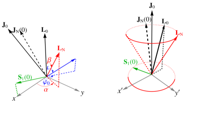
Figure 1: The inertial $\mathbf{L}_{0}$ and $\mathbf{J}_{0}$ frames whose $z$-axes are parallel to $\mathbf{L}_{\text{N}}(0)$ and $\mathbf{J}_{\text{2PN}}(0)$, respectively. We choose the $x$-axis of the $\mathbf{L}_{0}$ frame such that the initial spin of the primary component, $\mathbf{S}_{1}(0)$ lays in the $x$-$z$ plane. In this frame, we denote the spherical angles of $\mathbf{L}_{\text{N}}\equiv\mathbf{L}_{\text{N}}(t)$ (red arrow) by $\alpha$ and $\beta$. In the $\mathbf{J}_{0}$ frame, it is easier to discern the precession of $\mathbf{L}_{\text{N}}$ as it approximately traces out a cone per precession cycle (only approximately because $|\mathbf{L}_{\text{N}}|$ decreases due to radiation reaction, see Sec. II.3). We show such a cone in the right-hand panel along with its projection onto the plane perpendicular to $\mathbf{J}_{0}$. We also show $\mathbf{J}_{\text{N}}(0)$ as the dashed arrow, which is slightly different than our $\mathbf{J}_{0}$ which we explain in Sec. II.3. The blue arrow with the polar angles $(\iota,\varphi_{0})$ represents the line of sight to the detector.

Note that, for the purposes of data analysis and parameter estimation, we must restore $M$ to its physical units which we denote by $M_{\text{tot}}(M_{\odot})$. This is because the detection band of the GW interferometers is roughly between $20$ and $2000\,$Hz and the heavier binary systems merge at lower frequencies. Therefore, we parametrize our precessing binary inspirals using the following finalized set consisting of eight parameters

$$\{f_{0}(\text{Hz}),M_{\text{tot}}(M_{\odot}),q,\chi_{1},\chi_{2},\theta_{1},\theta_{2},\phi_{2}\},$$ (13)

where $f_{0}$ is the initial $(2,2)$-mode GW frequency marking the starting point of each inspiral.

II.3 Effects of precession

Spin-orbit precession occurs when the spins are not (anti)parallel to the orbital angular momentum. The main effect is a slow precession of $\mathbf{L}_{\text{N}}$ about an axis that is roughly aligned with $\mathbf{J}(0)$, but the true fixed axis depends on the order at which the precession ODEs are truncated, and the use of the appropriate solutions to those ODEs. For example, in Ref. Apostolatos et al. (1994), this axis is given by $\mathbf{J}_{0}\equiv\hat{\mathbf{J}}_{\text{N}}-\epsilon\,\hat{\mathbf{J}}_{\text{N}}\times\!\hat{\,\mathbf{L}}_{\text{N}}$ obtained from the NLO solutions while neglecting the spin-spin coupling. This $\mathbf{J}_{0}$ then indeed remains fixed. However, we neither truncate the ODEs at NLO, nor neglect the spin-spin coupling, therefore we choose not to use this choice for $\mathbf{J}_{0}$. As we solve the N4LO (2PN) equations here, which are obtained by imposing $\dot{\mathbf{J}}=\!\dot{\,\mathbf{L}}+\dot{\mathbf{S}}_{1}+\dot{\mathbf{S}}_{2}=0$ with $\mathbf{L}$ up to 3.5PN decaying under radiation reaction (see App. A), we have at best an approximate conservation of $\mathbf{J}_{\text{2PN}}$. Therefore, we set $\mathbf{J}_{0}=\mathbf{J}_{\text{2PN}}(0)$.

The decrease of $\mathbf{L}_{\text{N}}$ under radiation reaction results in a precession cone whose opening angle increases in time as illustrated in Ref. Apostolatos et al. (1994). Thus, the projection of $\!\hat{\,\mathbf{L}}_{\text{N}}$ orthogonal to $\mathbf{J}_{0}$ shows circularly outspiraling tracks as in Fig. 2. Furthermore, $\hat{\mathbf{J}}_{\text{N}}$ also precesses around, in fact, out-spirals around $\mathbf{J}_{0}$, which we also exhibit in Fig. 2. This spiralling behavior persists for PN-corrected $\mathbf{L}$ and $\mathbf{J}$, albeit with smaller precession cone opening angles for $\mathbf{J}$, as we show for $\hat{\mathbf{J}}_{2\text{PN}}$ in the figure. For three-dimensional versions of these, see Apostolatos et al.  Apostolatos et al. (1994) which still remains the most illustrative resource for understanding the qualitative behavior of precessing systems. Ref. Apostolatos et al. (1994) also provides a useful expression for the number of precession cycles when the masses are small and initial separation is large, i.e., $|\mathbf{L}_{\text{N}}|\gg|\mathbf{S}_{1}+\mathbf{S}_{2}|$,

$$N_{\alpha}\equiv\frac{\alpha}{2\pi}\approx 11\left(1+\frac{3m_{1}}{4m_{2}}\right)\frac{10M_{\odot}}{M_{\text{tot}}}\frac{10\,\text{Hz}}{f},$$ (14)

where, recall $M_{\text{tot}}$ is $M$ in solar masses.

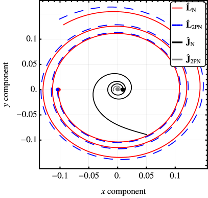
Figure 2: Tracks of the $x,y$ components of the Newtonian orbital ($\!\hat{\,\mathbf{L}}_{\text{N}}(t)$, red) and total angular [unit] momenta ($\hat{\mathbf{J}}_{\text{N}}(t)$, black) in the plane orthogonal to $\mathbf{J}_{0}=\mathbf{J}_{\text{2PN}}(0)$ for a binary with $M_{\text{tot}}=30M_{\odot},q=1,\chi_{1}=\chi_{2}=0.7,\theta_{1}=\theta_{2}=90^{\circ},$ and $\phi_{2}=135^{\circ}$ starting from the GW frequency of 20 Hz. We additionally show the components of the 2PN-corrected orbital angular momentum, $\!\hat{\,\mathbf{L}}_{\text{2PN}}$ (dashed blue), and the corresponding total angular momentum, $\hat{\mathbf{J}}_{\text{2PN}}$ (gray). The dots mark the starting positions for each vector. As described in the text, the various angular momenta spiral outward around the fixed axis $\mathbf{J}_{0}$, but $\hat{\mathbf{J}}_{\text{2PN}}$ outspirals much less than $\hat{\mathbf{J}}_{\text{N}}$ consistent with our use of solutions to the 2PN spin precession equations.

The precession of $\mathbf{L}_{\text{N}}$ induces amplitude modulations in the waveform and modifies the phase. The modulations depend strongly on the orientation of the orbit with respect to an observer’s line of sight. This is illustrated in Fig 3, where the gray curve is the precessing $(2,2)$ mode as seen by an observer lined up with $\mathbf{J}_{0}$ who receives less modulated GWs because $\mathbf{L}_{\text{N}}(t)$ tracks a circularly inspiralling path as depicted in Fig. 2 whereas the $\mathbf{L}_{0}$-frame observer sees emissions over an elliptically inspiralling track, hence resulting in larger amplitude variations. This means that the reference frame in which the incoming GWs are received (e.g., detector frame) plays a significant role in GW detection as using non-precessing waveform template banks to match-filter the signal can lead to a significant fraction of precessing signals being missed or dismissed as glitches Schmidt et al. (2012).

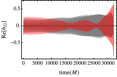
Figure 3: Precessing $(2,2)$ modes as viewed by observers whose line of sight is parallel to $\mathbf{L}_{0}$ (red) and to $\mathbf{J}_{0}$ (gray) for a binary system with $M_{\text{tot}}=30M_{\odot},q=1/5,\chi_{1}=\chi_{2}=0.7,\theta_{1}=\theta_{2}=\phi_{2}=135^{\circ}$ starting from 20 Hz. As discussed in the text, the $\mathbf{L}_{0}$-frame observers see much more pronounced amplitude modulations than their $\mathbf{J}_{0}$-frame counterparts.

Thus far, we have talked about simple precession dubbed so because both $\mathbf{L}$ and $\mathbf{S}$ precess around $\mathbf{J}$. However, when $\mathbf{L}+\mathbf{S}\approx 0$, a phenomenon known as transitional precession occurs in which $\mathbf{J}$ “tumbles” until radiation reaction decays $\mathbf{L}$ enough to take the system away from the $\mathbf{L}+\mathbf{S}\approx 0$ configuration Apostolatos et al. (1994). Since transitional precession requires careful fine-tuning of the parameters, it is expected to be a rare phenomenon Apostolatos et al. (1994); Buonanno et al. (2003) so we do not consider it here.

III Twisting non-precessing waveforms

Having conceptually introduced the twist operation, we next provide mathematical details. Our discussion here is mostly based on Refs. Boyle et al. (2011); Schmidt et al. (2012); Babak et al. (2017). Let us recall that $\alpha(t)$ and $\beta(t)$ are the azimuthal and polar angles of $\mathbf{L}_{\text{N}}(t)$ with respect to $\mathbf{L}_{0}=\mathbf{L}_{\text{N}}(0)$ and the third angle $\gamma(t)$ is obtained from $\dot{\gamma}=\dot{\alpha}\cos\beta$. The set $\{\alpha(t),\beta(t),\gamma(t)\}$ is all we need when transforming between the $\mathbf{L}_{\text{N}}(t)$ and $\mathbf{L}_{0}$ frames. Specifically, when going from our inertial $\mathbf{L}_{0}$ frame to the $\mathbf{L}_{\text{N}}(t)$-frame, we “forward”-Euler rotate using $R(\alpha,\beta,\gamma)\equiv R_{z}(\gamma)R_{y}(\beta)R_{z}(\alpha)$ where $R_{j}(\zeta_{k})$ represent rotations by the angles $\zeta_{k}$ with respect to the $j$ axis. In the following, we omit displaying the explicit time dependence of these angles and various other time-dependent quantities, e.g., $\mathbf{L}_{\text{N}}(t)$, which we restore when necessary.

Under the forward Euler rotation above, the gravitational-wave modes transform as follows

$$h_{\ell m}=\sum_{m^{\prime}=-\ell}^{\ell}h_{\ell m^{\prime}}\,D^{(\ell)}_{m^{\prime},m}(\alpha,\beta,\gamma)\,,$$ (15)

where $D^{(\ell)}_{m^{\prime},m}$ are Wigner’s D matrices which can be related to spin-weighted spherical harmonics via Goldberg et al. (1967)

$${}_{s}Y^{\ell m}(\theta,\phi)=(-1)^{m}\sqrt{\frac{2\ell+1}{4\pi}}D^{(\ell)}_{-m,s}(\phi,\theta,0).$$ (16)

Note that different versions of this equation exist in the literature due to conventions of Wigner D matrices. Here, we employ the definition introduced in Ref. Sakurai (1994)

$$D^{(\ell)}_{m^{\prime},m}(\alpha,\beta,\gamma)=e^{-im^{\prime}\alpha}e^{-im\gamma}d^{\ell}_{m^{\prime},m}(\beta),$$ (17)

where $d^{\ell}_{m^{\prime},m}(\beta)\in\mathbb{R}$ are the “little” D matrices given by

$$d^{\ell}_{m^{\prime},m}(\beta)= \sum_{k_{i}}^{k_{f}}(-1)^{k-m+m^{\prime}}$$

$$\times\frac{\sqrt{(\ell+m)!(\ell-m)!(\ell+m^{\prime})!(\ell-m^{\prime})!}}{k!(\ell+m-k)!(\ell-k-m^{\prime})!(k-m+m^{\prime})!}$$

$$\times\left[\cos\frac{\beta}{2}\right]^{2\ell-2k+m-m^{\prime}}\left[\sin\frac{\beta}{2}\right]^{2k-m+m^{\prime}},$$ (18)

where $k_{i}=\min(0,m-m^{\prime})$ and $k_{f}=\max(\ell+m,\ell-m^{\prime})$.

As explained in Sec. I, the key idea is to “unwrap” or twist aligned-spin waveforms generated in the $\mathbf{L}_{\text{N}}$ frame using Euler rotations. In order to transform from $\mathbf{L}_{\text{N}}$ to $\mathbf{L}_{0}$ frame, we “backward” Euler-rotate via the inverse rotation matrices: $R^{-1}=R(-\gamma,-\beta,-\alpha)$. Therefore, to twist we invert Eq. (15) Schmidt et al. (2011, 2012)

$$h^{\text{T}}_{\ell m}=\sum_{m^{\prime}=-\ell}^{\ell}h^{\text{NP}}_{\ell m^{\prime}}\,D^{(\ell)\ast}_{m^{\prime},m}(-\gamma,-\beta,-\alpha)\,,$$ (19)

where we introduced the superscripts T and NP to denote the twisted and the non-precessing waveforms, respectively. Using the standard identity $D^{(\ell)\ast}_{m^{\prime},m}=(-1)^{m^{\prime}-m}D^{(\ell)}_{-m^{\prime},-m}$ which translates to $(-1)^{m^{\prime}-m}d^{\ell}_{-m^{\prime},-m}(-\beta)=d^{\ell}_{m^{\prime},m}(-\beta)$ in Eq. (17), we obtain Schmidt et al. (2011, 2012); Hannam et al. (2014); Khan et al. (2019a)

$$h_{\ell m}^{\text{T}}(t)=e^{-im\alpha(t)}\sum_{m^{\prime}=-l}^{l}e^{im^{\prime}\gamma(t)}d^{\ell}_{m^{\prime},m}(-\beta(t))\,h_{lm^{\prime}}^{\text{NP}}(t)\,,$$ (20)

where we restored the time dependences.

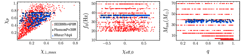
Figure 4: Our coverage of the eight-dimensional parameter space of precessing compact binary inspirals used in assessing the faithfulness of TEOBResumSP. The parameters $\{f_{0},q,M_{\text{tot}}\}$ span the space of nonspinning binaries, which is complemented by the set $\{\chi_{\text{eff},0},\chi_{p}\}$ or $\{\chi_{\text{eff},0},\chi_{\perp,\text{max}}\}$ that projects the five spin degrees of freedom in $\mathbf{S}_{1}(0),\mathbf{S}_{2}(0)$ [by design $\mathbf{S}_{1y}(0)=0$] to only two via Eqs. (9), (10), and (11). For our assessment, we considered 200 precessing binaries for the comparisons with NRSur7dq4 (blue triangles), IMRPhenomPv3HM (black squares), and 1230 binaries for comparisons with SEOBNRv4PHM (red dots). Note that some parameters are duplicate within the $\{f_{0},q,M_{\text{tot}}\}$ subset, hence there are fewer points in the middle and right panels than the rough total of 1230.

Note that the literature is replete with slightly different versions of Eq. (20) depending on: (i) Euler rotation conventions, (ii) Wigner D and spherical harmonic conventions, and (iii) the sign of the right-hand-side for the $\dot{\gamma}$ equation. Our definitions and conventions agree with Ref. Babak et al. (2017) (modulo the sign of $\gamma$) and our practical expression (20) agrees with Ref. Khan et al. (2019a) which interestingly disagrees with its updated version in Ref. Khan et al. (2019b), but then agrees with a recent version used in IMRPhenomXPHM Pratten et al. (2020b). We tested the performance of the alternate expression of Ref. Khan et al. (2019b) against ours in terms the $\ell=2$ detector strain mismatches of TEOBResumSP with SEOBNRv4PHM and NRSur7dq4. We found that the expression for the twist given by Eq. (20) performed better in the sense that it produced smaller mismatches. We delegate the details of this comparison to App. B.

In principle, one can also twist the non-precessing waveforms using the angles of PN-corrected $\mathbf{L}(t)$ with respect to $\mathbf{L}(0)$. Ref. Pan et al. (2014b) showed that the resulting differences in the twisted waveforms as compared with precessing NR waveforms are marginal, therefore we use only $\mathbf{L}_{\text{N}}(t)$ with respect to $\mathbf{L}_{\text{N}}(0)$ for TEOBResumSP.

We now have all the individual ingredients necessary to generate the precessing TEOBResumSP waveforms. The procedure for this operation is as follows:

1. Specify the initial parameters listed in Eq. (13).

2. Generate aligned-spin (non-precessing) $\ell=2$ waveform modes using TEOBResumS via the set of parameters $\{f_{0},M_{\text{tot}},q,\chi_{1},\chi_{2}\}$.

3. Solve the orbit-averaged spin precession ODEs (4a-4c) using SpinTaylorT4 resummed radiation reaction for $\dot{v}$.

4. Retrieve the spherical angles $\{\alpha(t),\beta(t)\}$ from the components of $\mathbf{L}_{\text{N}}(t)$ in the $\mathbf{L}_{\text{N}}(0)$ frame and subsequently obtain $\gamma(t)$ by solving $\dot{\gamma}=\dot{\alpha}\cos\beta$.

5. Construct the precessing $\ell=2$ TEOBResumSP modes via the twist formula (20).

Let us conclude this section with three remarks: (i) We can generate twisted waveforms in the $\mathbf{J}_{\text{N}}(0)$ frame as well as the $\mathbf{L}_{\text{N}}(0)$ frame, but this is slower because the solutions to the ODEs, which are solved in the $\mathbf{L}_{\text{N}}(0)$ frame, must be Euler-rotated to the $\mathbf{J}_{\text{N}}(0)$ frame at each time step. Therefore, for convenience we compare in the $\mathbf{L}_{\text{N}}(0)$ frame, but in principle we can straightforwardly rotate to the $\mathbf{J}_{\text{N}}(0)$ frame. (ii) It is possible to extend the above scheme by coupling the precession ODEs to TEOBResumS dynamics, i.e., by setting $\chi_{i}=\!\hat{\,\mathbf{L}}_{\text{N}}(t)\cdot\mathbf{S}_{i}(t)/m_{i}^{2}$ ($i=1,2$) at each time step of the aligned-spin EOB dynamics, where $\!\hat{\,\mathbf{L}}_{\text{N}}(t),\mathbf{S}_{i}(t)$ are obtained from the N4LO precession dynamics. This is similar to what is done in the precessing SEOBNRv3,v4 approximants, where aligned-spin modes with time-varying $\chi_{i}$ are twisted Pan et al. (2014b); Babak et al. (2017); Ossokine et al. (2020). (iii) For this initial version of TEOBResumSP, we truncate our precessing waveforms before the transition to ringdown. Attaching the ringdown portion to the inspiral-plunge-merger (IM) part of the precessing waveforms is quite a subtle procedure, especially in the time domain. For example, in SEOBNRv3P Babak et al. (2017), the ringdown waveforms are computed in the $\mathbf{J}(t_{\text{match}})$ frame, where $t_{\text{match}}$ approximates the merger time. Then, the ringdown waveform is attached to the precessing IM portions obtained by twisting the co-precessing modes to the $\mathbf{J}(t_{\text{match}})$ frame Babak et al. (2017). In the upgraded version, SEOBNRv4PHM Ossokine et al. (2020), the ringdown is attached in the co-precessing frame, which is less complicated to implement and less prone to numerical instabilities, thus is more appealing to us as a ringdown implementation. There is also the question of how far one can push the PN ODEs. The time domain IMRPhenomTP Estellés et al. (2020) approximant provides a prescription for extending $\alpha(t),\beta(t)$ into the ringdown regime (see Ref. Marsat and Baker (2018) for details of this prescription) and also uses the same implementation for $\alpha(t)$ as SEOBNRv4PHM. However, Ref. Estellés et al. (2020) remarks that this is a “simple implementation” that will be improved. In short, the ringdown attachment requires extreme care and detailed testing, that is why we leave it for the next version of TEOBResumSP.

IV Assessing the Twist: Comparisons with NRSur7dq4, IMRPhenomPv3HM and SEOBNRv4PHM

To assess the faithfulness of TEOBResumSP (henceforth TEOB), we compared the twisted TEOBResumS waveforms against precessing waveforms generated by the following three approximants: NRSur7dq4, IMRPhenomPv3HM, and SEOBNRv4PHM (henceforth, NRSur, Pv3HM, SEOB). We first considered a set of 200 precessing binaries consisting of “middle weight”, i.e., $35\leq M_{\text{tot}}\leq 37.5M_{\odot}$ BBHs, for a three-way comparison of TEOB with NRSur, Pv3HM, and SEOB. We then used the additional $1030$ more inspirals for an extended comparison with SEOB, which comprised of $100$ cases with BNS-like masses, a dozen cases with masses appropriate for black hole neutron star systems, approximately another 100 cases where one or both masses are in the lower mass gap, i.e., $\lesssim 5M_{\odot}$ Ozel et al. (2010); Farr et al. (2011); Abbott et al. (2020g), and the remaining cases involving typical stellar-mass BBHs. The non-precessing-binary parameters $\{f_{0},M_{\text{tot}},q\}$ corresponding to these 1230 cases are shown in Fig. 4, where we additionally show $\{\chi_{\text{eff},0},\chi_{\perp,\text{max}},\chi_{p}\}$ which project the remaining five spin degrees of freedom, $\mathbf{S}_{1}(0),\mathbf{S}_{2}(0)$, to just two (recall we set $\mathbf{S}_{1y}(0)=0$).

To assess TEOB, we first computed frequency-domain matches between TEOB-generated detector strains and those generated by $\{$NRSur, SEOB, Pv3HM$\}$ for the 200 inspirals, then extended the match computation to the expanded TEOB-SEOB comparison set. The match (or faithfulness) between two waveforms is computed by maximizing the following expression over initial time and phase shifts, $t_{0},\phi_{0}$ ​

$${\cal M}\equiv\max\limits_{t_{0},\phi_{0}}\frac{\langle h^{\mathtt{k}}|h^{\mathtt{T}}\rangle}{\sqrt{\langle h^{\mathtt{k}}|h^{\mathtt{k}}\rangle\langle h^{\mathtt{T}}|h^{\mathtt{T}}\rangle}},$$ (21)

where

$$\hskip 56.9055pt\langle h^{\mathtt{k}}|h^{\mathtt{T}}\rangle\equiv 4\Re\int_{f_{k}}^{f_{f}}\frac{\tilde{h}^{\mathtt{k}}(f)\,\tilde{h}^{\mathtt{T}\ast}(f)}{S_{n}(f)}df$$ (22)

is the inner product between the Fourier transforms of the GW strain, $\tilde{h}^{\mathtt{k}},\tilde{h}^{\mathtt{T}}$, weighted by the one-sided power spectral density (PSD) $S_{n}(f)$ of the detector noise with T denoting TEOB and k = NRSur, Pv3HM, SEOB. For the PSD, we use Advanced LIGO’s “zero-detuned high-power” design sensitivity of Ref. aLI . We set $f_{i}=1.05f_{0}$, where recall $f_{0}$ is the initial non-precessing $(2,2)$ mode frequency. As for $f_{f}$, since the current version of TEOB does not include ringdown, we opted for a suitable cutoff that is near the peak of the twisted (2,2) mode, but slightly less: $f_{f}=0.95f^{22}_{\text{peak}}$, to err on the side of caution. There are many subtleties and complications in selecting the proper peak when non-precessing modes first get “mixed up” in the twist formula, after which the resulting precessing modes further get mixed up in the mode sum (26) for the GW strain. As Ref. Babak et al. (2017) discusses in their App. D, there may be cases in which several local peaks may be found, or none at all.

In the time domain, the GW strain in a detector reads

$$h(t)= F_{+}(\theta_{s},\phi_{s},\psi_{s})h_{+}(t,\iota_{s},\varphi_{0})$$

$$+F_{\times}(\theta_{s},\phi_{s},\psi_{s})h_{\times}(t,\iota_{s},\varphi_{0}),$$ (23)

where $F_{+,\times}$ are the detector antenna pattern functions given by

$$F_{+}(\theta,\phi,\psi) =\frac{1+\cos^{2}\theta}{2}\cos 2\phi\cos 2\psi-\cos\theta\sin 2\phi\,\sin 2\psi,$$ (24)

$$F_{\times}(\theta,\phi,\psi) =\frac{1+\cos^{2}\theta}{2}\cos 2\phi\sin 2\psi+\cos\theta\sin 2\phi\,\cos 2\psi.$$ (25)

In Eq. (23), $\theta_{s},\phi_{s}$ are the sky-position angles, and $\psi_{s}$ is the polarization angle of the GWs in the detector frame. $h_{+,\times}$ are the standard GW polarizations which come from the following mode sum

$$h_{+}-ih_{\times}=\frac{1}{D_{L}}\sum_{\ell=2}^{\infty}\sum_{m=-\ell}^{\ell}h_{\ell m}(t)\,{}_{-2}Y^{\ell m}({\iota_{s}},\varphi_{0}),$$ (26)

where $D_{L}$ is the distance to the source, which we set to $100\,$Mpc, ${}_{-2}Y^{\ell m}$ are the (spin = $-2$)-weighted spherical harmonics, $\iota_{s}$ is the orbital inclination, and $\varphi_{0}$ is the azimuthal angle between the $x$-axis of the $\mathbf{L}_{\text{N}}(0)$ frame and the projection of the detector line-of-sight vector onto the plane perpendicular to $\mathbf{L}_{\text{N}}(0)$ (see Fig. 1). Formally, $h(t)$ is obtained from a sum over all $\ell,m$ modes, but here, we suffice with the $\ell=2$ mode. We will incorporate the available $\ell>2$ modes, which recently got upgraded Nagar et al. (2020), in the next version of TEOBResumSP. Note that EOBNR approximants do not model $m=0$ modes, so we set the (2,0) mode equal to zero.

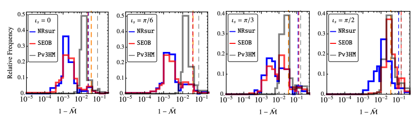
Figure 5: The distribution the three-angle ($\psi_{s},\theta_{s},\phi_{s}$) averaged mismatch, $1-\bar{{\cal M}}$, between TEOBResumSP and NRSur7dq4 (blue), SEOBNRv4PHM (red), and Pv3HM (grey) for the 200 precessing inspirals of Sec. IV.1 for orbital inclinations of $\iota_{s}=0,\pi/6,\pi/3,\pi/2$. The vertical orange dashed line marks the mismatch corresponding to $0.035$. The dashed blue, red, and black vertical lines mark the 95th percentile of each set.

It has become standard in waveform comparisons to use ${\cal M}=0.965$ as a benchmark. This cutoff translates to the loss of roughly 10% of events due to waveform systematics Owen (1996); Flanagan and Hughes (1998). We also employ this threshold and its mismatch counterpart $1-{\cal M}=0.035$ which we plot either as a horizontal or vertical dashed orange line in many of our subsequent figures.

IV.1 Summary of the main comparisons

For our main comparison, we considered a set of 200 precessing compact binary inspirals plotted as the blue-black dots in the parameter space figure 4. For each inspiral we compared TEOB to $\{$NRSur, SEOB, Pv3HM$\}$ by computing the detector strain matches using Eq. (21). As NRSur has been shown to be better than 99% faithful to NR simulations for $>95\%$ of the cases in its extrapolation space Varma et al. (2019), it has become the current gold standard. Therefore, we picked the parameters for our 200 cases to be well within NRSur’s domain of interpolation, i.e., $1/4\leq q\leq 1$ and $\chi_{1},\chi_{2}\leq 0.8$ Varma et al. (2019). In order to maximize the number of orbital cycles, hence the number of precession cycles, we set $f_{0}\in[35,40]\,$Hz and $M_{\text{tot}}\in[35,40]M_{\odot}$. Making these values any smaller tended to hit the low frequency bound of NRSur, and setting them higher would miss the one, or at best two, precession cycles that we expect. We further set $\chi_{1}=\chi_{2}=0.75$ since higher spins tend to lead to more pronounced precession, thus posing a tougher challenge for the precessing approximants.

For the $h(t)$ computation in Eq. (23) , we used a grid of $\iota_{s}=\{0,\pi/6,\pi/3,\pi/2\}$ and $\psi_{s}=\{0,\pi/8,\pi/4,3\pi/8\}$ with random values assigned for $\varphi_{0}\in[0,2\pi)$ at each value of $\{\iota_{s},\psi_{s}\}$. For the sky angles $\{\theta_{s},\phi_{s}\}$, we employed a grid with spacing ${\pi/4}$. At each point in the four-angle grid, we generated $h(t)$ using TEOB, NRSur, SEOB, and Pv3HM. This resulted in a total of $4\times 200\times 4\times 4\times 4\times 8\sim 4\times 10^{5}$ strains from which we computed the matches between TEOB and $\{$NRSur, SEOB, Pv3HM$\}$ via Eq. (21) using the Python library PyCBC Nitz et al. (2020).

For the $\sim 10^{5}$ TEOB-NRSur matches, we found that 91% were greater than 0.965 and less than 3% of the sample yielded ${\cal M}<0.9$ the majority of which happened with inclinations of $\iota=\pi/3$ and $\pi/2$. Similarly, 85% of the TEOB-SEOB matches and 77% of the TEOB-Pv3HM matches were greater than 0.965. These percentages remained within $\pm 1\%$ when we switched from an evenly spaced $\{\theta_{s},\phi_{s}\}$ grid to a random one as well as when we repeated the entire computation with new random values for $\varphi_{0}$. To summarize our main results, we introduce the three-angle averaged match, $\bar{{\cal M}}$ as follows. Given a set of binary parameters, we fix $\iota_{s},\varphi_{0}$ then compute the match ${\cal M}_{ijk}$ between a given pair of approximants at each of the $4\times 4\times 8=128$ points in the $\{\psi_{si},\theta_{sj},\phi_{sk}\}$ grid. $\bar{{\cal M}}$ is then just the straightforward discrete mean of ${\cal M}_{ijk}$. Note that since by definition $0\leq{\cal M}\leq 1$ and our main threshold is ${\cal M}=0.965$, the averaging tends to produce lower percentages of $\bar{{\cal M}}>0.965$ cases. Therefore, we present percentages over our entire match set, but use $\bar{{\cal M}}$ in our figures.

In Fig. 5 we present the distributions of the three-angle averaged mismatch, $1-\bar{{\cal M}}$, between TEOB and the validation approximants NRSur, SEOB, and Pv3HM for $\iota_{s}=\{0,\pi/6,\pi/3,\pi/2\}$. As can be seen in the figure, the majority of the mismatches lays to the left of $0.035$ represented by the vertical dashed orange line. The vertical dashed $\{$blue, red, gray$\}$ lines respectively represent the 95th percentile TEOB-$\{$NRSur, SEOB, Pv3HM$\}$ mismatches. Clearly, for $\iota\leq\pi/6$, TEOB matches NRSur and SEOB better than 0.965 for more than 95% of the cases. For the TEOB-Pv3HM matches, this is roughly 86%. The shift of the peak of $1-\bar{{\cal M}}$ from $10^{-3}$ to $10^{-2}$ as $\iota_{s}$ increases is also evident in the figure for the TEOB-NRSur (blue) and TEOB-SEOB (red) histograms, whereas for the TEOB-Pv3HM distribution (gray) this shift is much less pronounced with the peak of the distribution also remaining much narrower

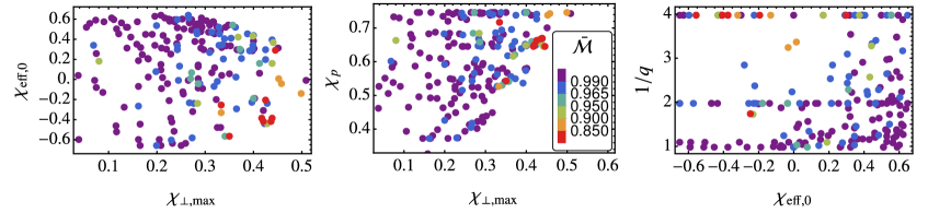
Figure 6: Two-dimensional scatter plots of the three-angle averaged match, $\bar{{\cal M}}$, between TEOBResumSP and NRSur7dq4 for the 200 precessing compact binary inspirals as “seen” at an orbital inclination of $\iota_{s}=\pi/3$. For this figure, we opted for $1/q$ to better relate to values more familiar in the NR community. The cooler colors (purple, blue) represent cases with $\bar{{\cal M}}\geq 0.965$ while the warmer colors (orange, red) represent $\bar{{\cal M}}\leq 0.9$. See Sec. IV.2 for details as to why the match degrades in certain regions. The distribution of the colors is roughly the same for $\iota_{s}=\pi/6,\pi/2$, albeit with very few “hot” dots for the former and about the same number for the latter.

for all inclinations.

The deterioration of TEOB’s agreement with the other approximants for increasing $\iota_{s}$ is expected since the precessing $(2,\pm 1),(2,0)$ modes contribute more to the GW strain as $\iota_{s}$ increases. The disagreements in these modes stem from disagreements in the non-precessing $(2,\pm 1),(2,0)$ modes. For example, we found that while all, but one, non-precessing $(2,2)$ modes of TEOBResumS matched their non-precessing NRSur counterparts to better than 0.99, only 60% of the non-precessing $(2,1)$ modes achieved matches greater than $0.965$. We further confirmed that most of the worst strain mismatches do indeed come from cases where the non-precessing $(2,1)$ mode matches between TEOB and the validation approximants are less than 0.9. This is consistent with the findings of Ref. Ramos-Buades et al. (2020), where the effects of mismodelling the non-precessing $(2,1)$ and higher modes were systematically investigated. As expected, we also found out that the worst matching cases between TEOB and the validation approximants have $0.65\lesssim\chi_{p}\leq 0.75$ and $q\lesssim 1/3$ with the majority having $q=1/4$.

Overall, for the set of precessing compact binary inspirals considered in this section with $0.3\lesssim\chi_{p}\leq 0.75$, SEOB showed the best agreement with NRSur with only 6.9% of the $\sim 10^{5}$ matches below 0.965. This percentage was $14\%$ for NRSur-Pv3HM and 18% for SEOB-Pv3HM matches. For the inclination of $\iota_{s}=\pi/2$, Pv3HM matched NRSur best with 91% of the cases yielding ${\cal M}>0.95$, whereas TEOB and SEOB had 88.6% and 86.6% of these cases yield ${\cal M}>0.95$, respectively. These differences once again highlight the importance of having several different waveform approximants. We present additional details of TEOB’s performance against $\{$NRSur, Pv3HM, SEOB$\}$ in the next subsections.

IV.2 Comparisons with NRSur7dq4 waveforms

For the $\sim 10^{5}$ TEOB-NRSur matches that we computed, we found that 74.1, 91.1, 93.8% yielded ${\cal M}>0.99,0.965,0.95$, respectively. Within the four $\iota_{s}=0,\pi/6,\pi/3,\pi/2$ subsets, 97.6, 95.5, 86.7, 84.7% yielded ${\cal M}>0.965$. Similarly, 97.0% of the $q<1/4$ matches gave ${\cal M}>0.965$ in contrast to 78.1% of the $q=1/4$ cases. Of the $q=1/4$ cases, about 94% and 86% of the $\iota_{s}=0,\pi/6$ subsets yielded ${\cal M}>0.965$ as opposed to only about 2/3 of the $\iota_{s}=\pi/3,\pi/2$ subsets giving ${\cal M}>0.965$.

The increase of mismatch with decreasing mass ratio and increasing orbital inclination is a direct outcome of the increasing mismatch between the precessing $(2,\pm 1),(2,0)$ modes of TEOB and NRSur. This disagreement, in turn, stems mostly from the less-than-ideal agreement between the non-precessing $(2,\pm 1)$ modes TEOB and NRSur mentioned in Sec. IV.1. Additionally, TEOB sets $h_{20}^{\text{NP}}=0$ which NRSur does not, but the mismatch due to this assignment is subdominant as the amplitude of $h_{20}^{\text{NP}}$ is orders of magnitude smaller than the amplitude of $h_{21}^{\text{NP}}$. As a test, we replaced $h_{21}^{\text{NP},\mathtt{TEOB}}$ with $h_{21}^{\text{NP},\mathtt{NRsur}}$ for a few cases and observed that the resulting TEOB-NRSur match improved, verifying our above hypothesis that the non-precessing $(2\pm 1)$ modes are mostly responsible for the high-inclination, low-$q$ mismatches.

We also explored how the TEOB-NRSur match behaves across the precessing binary parameter space. In Fig. 6, we show two-dimensional scatter plots of the match against $\chi_{\text{eff},0},\chi_{p},\chi_{\perp,\text{max}}$, and $1/q$ for $\iota_{s}=\pi/3$. As can be deduced from the middle panel of the figure, the match worsens for larger values of $\chi_{p},\chi_{\perp,\text{max}}$, i.e., stronger precession, indicated by the “warmer” colors (red, orange). Also evident in the right panel is the aforementioned degradation of the match for the $q=1/4$ cases. Interestingly, the match also worsens for more negative values $\chi_{\text{eff},0}$ hinted both in the left and right panels. This again relates back to the mismatch in the non-precessing $(2,\pm 1)$ modes. These trends persist for $\iota_{s}=\pi/6,\pi/2$, albeit less pronounced for the former.

Figure 7: Three-angle averaged mismatch, $1-\bar{{\cal M}}$ between TEOBResumSP and NRSur7dq4 vs $\chi_{\perp,\text{max}}$ (left panel, blue dots) and $\chi_{p}$ (right panel, teal dots) for $\iota_{s}=\pi/6$. The horizontal dashed black, orange, and gray lines represent mismatches of 0.01, 0.035, and 0.1, respectively. The mismatch seems to depend more strongly on $\chi_{\perp,\text{max}}$ than $\chi_{p}$, which suggests that $\chi_{\perp,\text{max}}$ may somehow expose a systematic error in TEOBResumSP resulting from twisting constant-spin non-precessing waveforms as opposed to time-varying ones.

As an interesting side note, we compared in Fig. 7 how $1-\bar{{\cal M}}$ changes when plotted against $\chi_{p}$ versus against $\chi_{\perp,\text{max}}$ for $\iota_{s}=\pi/6$. The [semilog] plots hint that $1-\bar{{\cal M}}$ shows a vague exponential dependence on $\chi_{\perp,\text{max}}$, but not on $\chi_{p}$. This trend persists for other inclinations, albeit with more outliers for larger values of $\iota_{s}$. The trend also shows in the mismatches of TEOB with Pv3HM as we illustrate in the next subsection. The trend even persists for NRSur-Pv3HM and NRSur-SEOB mismatches, albeit less clearly, but again more strongly for small $\iota_{s}$ as in TEOB-NRSur mismatches. This suggests that $\chi_{\perp,\text{max}}$ might somehow expose a systematic error in the way that the approximants generate their precessing waveforms. A more detailed study is required to firmly establish this (or refute it). Nonetheless, based on these findings and given that the values for $\chi_{\perp,\text{max}}$ seem less degenerate than $\chi_{p}$ (at least for the 200 cases here), we believe that $\chi_{\perp,\text{max}}$ may be useful in future parameter estimation studies. In the least, it seems to encode the strength of precession.

IV.3 Comparisons with IMRPhenomPv3HM waveforms

Of the $\sim 10^{5}$ TEOB-Pv3HM matches, 77.6% are greater than $0.965$ and 86.4% greater than $0.95$. The percentage of matches greater than 0.965 in the four $\iota_{s}=0,\pi/6,\pi/3,\pi/2$ subsets are 91.4, 87.2, 71.1, 60.7, respectively. As with the NRSur comparisons, the $q=1/4$ subset has fewer ${\cal M}>0.965$ cases, 45% of the set, than the $q<1/4$ subset, 87.6%. Within the $q=1/4$ subset, 65% and 57% of the $\iota_{s}=0,\pi/6$ subsets have ${\cal M}>0.965$ as opposed to only 36%, 22% for the $\iota_{s}=\pi/3,\pi/2$ subsets (these last two percentages are greater than 50% when considering ${\cal M}=0.95$).

The way TEOB compares with Pv3HM is roughly consistent with the way it compares with NRSur, albeit with lower percentages of ${\cal M}>0.965$ cases overall and within the chosen subsets. This consistency is evident when comparing Fig. 8 with Fig. 6, i.e, the two-dimensional scatter plots of $\bar{{\cal M}}$ for $\iota_{s}=\pi/3$. In both figures, many of the red dots are located at the same positions in the $\{\chi_{\text{eff},0},\chi_{\perp,\text{max}},\chi_{p},1/q\}$ space, with some orange dots of Fig. 6 also having become red. In fact, the major difference between the two figures is the “reddening” of the dots, consistent with Fig. 5 where the position of the peak of the distribution of TEOB-NRSur mismatches is roughly an order of magnitude smaller than the peak of the distribution of TEOB-Pv3HM mismatches, hence the domination of Fig. 6 by the purple dots, and of Fig. 8 by the blue dots. We should re-emphasize that it is not just TEOB that produces increasing mismatches for small $q$ and large $\chi_{p},\iota_{s}$. In fact, Pv3HM exhibits a similar degradation in its matches with NRSur, as does SEOB (but less so). When compared with each other, all approximants show increasing disagreements in this challenging region requiring excellent match of all precessing modes, not just the $(2,2)$ mode.

In Fig. 9 we plot the three-angle averaged mismatch between TEOB-Pv3HM against $\chi_{\perp,\text{max}}$ and $\chi_{p}$ for $\iota_{s}=\pi/6$. As in Fig. 7, a vague exponential relation between $1-\bar{{\cal M}}$ and $\chi_{\perp,\text{max}}$ can be discerned. Analogous to the TEOB-NRSur comparisons, this relation persists for other values of $\iota_{s}$. As we already discussed the implications of this relation in the previous section, we move on to comparisons of TEOB with SEOB.

IV.4 Extensive comparisons with SEOBNRv4PHM waveforms

SEOBNRv4PHM is the latest precessing approximant within the SEOBNR family. As the upgrade to SEOBNRv3 Pan et al. (2014b); Babak et al. (2017), it incorporates precession in higher modes up to $\ell=5$ Ossokine et al. (2020). The precession in SEOBNRv4PHM (also in v3) is coupled to the aligned-spin EOB dynamics so that the resulting aligned-spin waveforms in the co-precessing frame are obtained from time-dependent $\chi_{1},\chi_{2}$. Most recent comparisons using approximately 1500 precessing SXS simulations have yielded SEOBNRv4PHM-NR matches of $>0.97$ for $>94\%$ of the cases with the higher modes included Ossokine et al. (2020). Note that these currently consist of only the $(3,\pm 3),(4,\pm 4),(5,\pm 5)$ modes lacking the important and more challenging $(3,\pm 2)$ and $(4,\pm 3)$ modes Ossokine et al. (2020). Moreover, SEOBNRv4PHM is not yet calibrated to NR waveforms in the precessing sector, but only to the aligned-spin waveforms. Nonetheless, along with IMRPhenomXPHM

Figure 8: Same as Fig. 6, but now for matches between TEOBResumSP and IMRPhenomPv3HM once again for $\iota_{s}=\pi/3$. Note that many of the red dots here are the same as those of Fig. 6. This similarity persists for all values of $\iota_{s}$.

Pratten et al. (2020b), SEOBNRv4PHM is currently one of the most NR-faithful, non-surrogate precessing approximants.

Since SEOBNRv4PHM does not suffer from the current parameter limitations of NRSur7dq4, we used a larger set of 1230 precessing inspirals with the parameters spanning greater ranges. In particular, for the key parameters, we have: $0\leq\chi_{p}\leq 0.993,f_{0}\geq 20\,\text{Hz},0.1\leq q\leq 1$, and $3M_{\odot}\leq M_{\text{tot}}\leq 70M_{\odot}$ (see Fig. 4). We realize that comparing cases with $\chi_{p}$ in excess of 0.9 is rather ambitious, especially since SEOB has been tested against NR only up to this limit Ossokine et al. (2020). Nonetheless, Ref. Ossokine et al. (2020) also presented an SEOB-Pv3HM comparison up to $\chi_{p}\lesssim 0.99$ so we proceed in the same spirit.

Within this expanded set, 200 cases have already been partly discussed in Secs. IV.1, where we reported the TEOB-SEOB matches and their distribution in Fig. 5. Here, we add to this an expanded set of 1030 cases for which we once again computed the $\{\psi_{s},\theta_{s},\phi_{s}\}$-averaged matches, $\bar{{\cal M}}$, between TEOB and SEOB for inclinations of $\iota_{s}=0,\pi/6,\pi/3$. As we discuss below, we leave the $\iota_{s}=\pi/2$ comparison to future work. As before, we used a $4\times 4\times 8$ grid for $\{\psi_{s},\theta_{s},\phi_{s}\}$ while assigning random values to $\varphi_{0}$. This amounted to $128\times 1030\approx 1.3\times 10^{5}$ matches computed for each inclination. We set $D_{L}=100\,$Mpc as before.

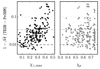
Figure 9: The three-angle averaged mismatch, $1-\bar{{\cal M}}$ between TEOBResumSP and IMRPhenomPv3HM plotted against $\chi_{\perp,\text{max}}$ and $\chi_{p}$ for $\iota_{s}=\pi/6$. As in Fig. 7, the mismatch increases with increasing $\chi_{\perp,\text{max}}$ (black dots, left panel), but seems to depend less strongly on $\chi_{p}$ (gray dots, right panel). The horizontal dashed black, orange, and gray lines represent $1-\bar{{\cal M}}=0.01,0.035,0.1$, respectively.

For the full set of 1230 cases, 90% of the $\iota_{s}=0,\pi/6$ matches are above 0.965 with this percentage dropping to 75% for $\iota_{s}=\pi/3$. We checked that these percentages remained unchanged (to less than 0.5%) when using randomly assigned values for $\theta_{s},\phi_{s}$ instead of a grid with spacing of $\pi/4$. Part of the reason for the increased disagreement with respect to the TEOB-NRSur comparison is the fact that now roughly 7.5% of the 1230 non-precessing TEOBResumS-SEOB (2,2)-mode matches are less than 0.965, whereas there was a single non-precessing TEOBResumS-NRSur (2,2) mode match less than 0.99 out of 200 cases. Some of this (2,2)-mode disagreement is due to the increased range of $q$ down to 0.1, for which we find that there are indeed increased occurrences of non-precessing (2,2) mode matches less than 0.965 for $q\lesssim 0.2$. Moreover, 42% of the non-precessing (2,1) mode matches are also less than 0.965. This latter disagreement manifests a more prominent mismatch in the precessing $(2,\pm 1),(2,0)$ modes which matter more for cases with strong precession and larger inclination. Therefore, given that nearly 60, 25% of the 1230 cases have $\chi_{p}\geq 0.5,0.7$ with a mean of 0.55, the degradation we observe in $\bar{{\cal M}}$ when going from $\iota_{s}=0,\pi/6$ to $\iota_{s}=\pi/3$ is not surprising. A similar disagreement has been shown between SEOB and Pv3HM for $\chi_{p}\gtrsim 0.7$ at $\iota_{s}=\pi/3$ Ossokine et al. (2020), but a similar $\iota_{s}=\pi/2$ comparison was not reported there. For our set, we find that $\bar{{\cal M}}$ degrades even more severely when going from $\iota_{s}=\pi/3$ to $\pi/2$ with only half the matches greater than 0.85. Again the culprit mostly seems to be the precessing (2,0) mode for which the TEOB-SEOB matches are mostly in the range of 0.6 to 0.8. As this requires further investigation, we limit our comparisons here to $\iota_{s}\leq\pi/3$.

In Fig. 10, we show the distribution of the TEOB-SEOB three-angle-averaged mismatches, $1-\bar{{\cal M}}$,

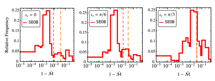
Figure 10: The distribution the three-angle ($\psi_{s},\theta_{s},\phi_{s}$) averaged mismatch, $1-\bar{{\cal M}}$, between TEOBResumSP and SEOBNRv4PHM for the additional 1030 precessing inspirals for orbital inclinations of $\iota_{s}=0,\pi/6,\pi/3$. The vertical orange dashed line marks the mismatch corresponding to $0.035$. The vertical dashed red line marks the 95th percentile. The parameters for the 1030 cases are represented by the red dots in Fig. 4 that do not overlap with the blue, black markers.

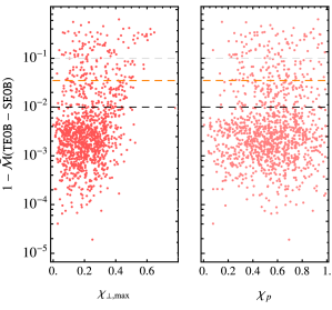
Figure 11: The three-angle averaged mismatch, $1-\bar{{\cal M}}$ between TEOBResumSP and SEOBNRv4PHM plotted against $\chi_{\perp,\text{max}}$ (red) and $\chi_{p}$ (pink) for $\iota_{s}=\pi/6$. Though the trend seen in Figs. 7 and 9 with respect to $\chi_{\perp,\text{max}}$ seems to have gotten mostly “buried”, its plot still looks like less of a random scatter than the corresponding $\chi_{p}$ plot. The horizontal dashed black, orange, and gray lines represent $\bar{{\cal M}}=0.99,0.965,0.9$, respectively.

for the three inclinations. As can be seen in the figure, for $\iota_{s}=0$ and $\pi/6$, the mismatches have a tall, narrow distribution centered at roughly $2\times 10^{-3}$, which becomes broader and shifts to roughly $2\times 10^{-2}$ for $\iota_{s}=\pi/3$.

We also checked whether or not the $\ln(1-\bar{{\cal M}})$ vs $\chi_{\perp,\text{max}}$ trend of Figs. 7 and 9 persisted for the entire set of 1230 TEOB-SEOB matches, which we show in Fig. 11 for $\iota_{s}=\pi/6$, where we also plot $\ln(1-\bar{{\cal M}})$ vs $\chi_{p}$ as before. It is clear from the new figure that the vague trend we had previously discerned has more or less disappeared as the set size increased by roughly an order of magnitude as well as the range of $q,f_{0},M_{\text{tot}}$. This is not unexpected since more cases with greater range of parameters may increase the potential causes of disagreement between waveform approximants, thus burying the rough trend of Figs. 7 and 9. Indeed, the alternate version of Fig. 11 made using only the 200 cases of Secs. IV.1-IV.3 looks very similar to Figs. 7 and 9. The proper way to check for this trend is to compare precessing waveforms for only the cases for which the non-precessing modes show excellent agreement (e.g., matches $>$ 0.99) then slowly increase $\theta_{1},\theta_{2}$ while keeping all other parameters unchanged, thus only increasing $\chi_{\perp,\text{max}}$ and $\chi_{p}$. The resulting plots of $\ln(1-\bar{{\cal M}})$ vs $\chi_{\perp,\text{max}}$ and $\chi_{p}$ would be much more conclusive as to whether or not the trend with respect to $\chi_{\perp,\text{max}}$ exists. We leave this for future work.

Since we greatly expanded the ranges of a few parameters, we investigated how this may affect the TEOB-SEOB matches by plotting them against $\chi_{p},q,\chi_{\text{eff},0}$, and the inspiral time $T_{\text{insp}}$, in Fig. 12 for $\iota_{s}=\pi/3$. As in Figs. 6, 8 we observe increasing mismatches for larger values of $\chi_{p}$ (and $\chi_{\perp,\text{max}}$) and more negative values of $\chi_{\text{eff},0}$. Additionally, the matches worsen for $q\lesssim 0.25$. This is not unexpected as it is known that the mismatch between the non-precessing TEOBResumS and SEOBNRv3 increases as $q$ decreases Nagar et al. (2018), but a similar investigation between TEOBResumS and SEOBNRv4 has not yet been conducted. However, we have already mentioned that we have observed some $q\lesssim 0.2$ cases with the TEOBResumS-SEOB non-precessing (2,2) mode matches less than 0.965.

The inspiral time seems to have no affect on the matches, up to the longest inspirals considered here, i.e., 25 seconds. The corresponding plots for $\iota_{s}=0,\pi/6$ contain the same regions of degrading matches, albeit with very few orange and red dots. Combining Figs. 6, 8 and 12, we can conclude that the most challenging “corner” of the parameter space for TEOBResumSP to match other precessing approximants is the three-dimensional $q\lesssim 0.25,\chi_{\text{eff},0}\lesssim-0.5,\chi_{p}\gtrsim 0.6$ region. The small-$q$, large-$\chi_{p}$ corner also seems to be a region of increased mismatch between SEOB and Pv3HM as shown in Fig. 14 of Ref. Ossokine et al. (2020) and also between Pv3HM and NR as hinted by Ref. Khan et al. (2019b) though there were only three NR simulations for the comparison. Increasing mismatches for larger $\chi_{p}$ values and $q\leq 1/5$ have also been observed between IMRPhenomXPHM and NR simulations Pratten et al. (2020b).

V Conclusions

In this article, we introduced TEOBResumSP: the precessing upgrade to TEOBResumS. Currently, TEOBResumSP generates precessing $\ell=2,m\in[-2,2]$ modes by Euler-rotating non-precessing (aligned, constant spin) TEOBResumS modes from the instantaneous, non-inertial $\mathbf{L}_{\text{N}}(t)$ frame to the inertial $\mathbf{L}_{\text{N}}(0)$ frame. This frame rotation, given by Eq. (20), is performed with Wigner’s D matrices. As it is, TEOBResumSP generates precessing modes only up to merger taken to be the peak of the twisted (2,2) mode.

We assessed the faithfulness of TEOBResumSP by computing the polarization-declination-right-ascension averaged $\ell$=2 detector strain matches between TEOBResumSP and $\{$NRSur7dq4, IMRPhenomPv3HM, SEOBNRv4PHM$\}$ for 200 binaries at orbital inclinations of $\iota_{s}=0,\pi/6,\pi/3$, and $\pi/2$. We further compared TEOBResumSP against SEOBNRv4PHM for an additional set of 1030 binaries.

We also introduced a new parameter, $\chi_{\perp,\text{max}}$, in Eq. (11), which encodes the strength of precession. We showed in Secs. IV.2-IV.4 how the waveform mismatch vaguely follows a trend roughly proportional to $e^{\chi_{\perp,\text{max}}}$. Additionally, at least for the precessing binaries used in this article, the values of $\chi_{\perp,\text{max}}$ are less degenerate than $\chi_{p}$, which we think would be a desirable property.

In summary:

1. TEOBResumSP matched NRSur7dq4 to better than 0.99 for 74% and better than 0.965 for 91% of the 200 cases with $\chi_{p}$ ranging up to $0.75$. Even for $\iota_{s}=\pi/2$, 85% of the matches were greater than 0.965.

2. For the same cases, 85% of the TEOBResumSP-SEOBNRv4PHM and 77% of the TEOBResumSP-IMRPhenomPv3HM matches exceeded 0.965 with higher percentages for low-inclination matches, and lower ones for high inclinations.

3. For the additional set consisting of 1030 binaries, 89% of the $\iota_{s}=0,\pi/6$, TEOBResumSP-SEOBNRv4PHM matches were greater than 0.965, which dropped to 73% for $\iota_{s}=\pi/3$.

4. Perhaps not surprisingly, the agreement between TEOBResumSP and $\{$NRSur7dq4, IMRPhenomPv3HM, SEOBNRv4PHM$\}$ worsens for cases with stronger precession indicated by larger values of $\chi_{p}$ (and $\chi_{\perp,\text{max}}$). Additionally, there is increasing disagreement for binaries with large negative spins and small mass ratios. In particular, the three-dimensional region of the parameter space bounded roughly by $\chi_{p}\gtrsim 0.5,\chi_{\text{eff},0}\lesssim-0.3,q\lesssim 0.25$ has the densest population of matches less than 0.85.

The major cause of the disagreement is the mismatch of the non-precessing modes. Any case for which the non-precessing (2,2) mode, $h_{22}^{\text{NP}}$, matches less than 0.965 will yield strain matches of $\lesssim 0.965$ as $h_{22}^{\text{NP}}$ contributes the most to the precessing (twisted) (2,2) mode which in turn is the dominant mode in the strain for most inclinations. While there is only one non-precessing (2,2) mode match of less than 0.99 between TEOBResumSP and NRSur7dq4 for the set of 200 binaries, 7% of the 1230 TEOBResumSP-SEOBNRv4PHM non-precessing (2,2) mode matches are less than 0.965. These percentages increase to roughly 40% and 42% for the matches of $h_{21}^{\text{NP}}$ for the same sets above. As $h_{21}^{\text{NP}}$’s contribution to the strain increases with respect to that of the $h_{22}^{\text{NP}}$’s with increasing inclination, the mismatches of $h_{21}^{\text{NP}}$ affect the high-inclination cases more as confirmed by our findings.

One possible explanation for the increase in TEOBResumSP-NRSur7dq4 and TEOBResumSP-SEOBNRv4PHM mismatches with increasing $\chi_{p}$ is the fact TEOBResumSP twists constant-spin, non-precessing waveforms, i.e., $\mathbf{S}_{1}(t)=\chi_{1}m_{1}^{2},\mathbf{S}_{2}(t)=\chi_{2}m_{2}^{2}$, whereas both NRSur7dq4 and SEOBNRv4PHM twist so-called co-precessing waveforms with time-varying $\mathbf{S}_{1}(t),\mathbf{S}_{2}(t)$ obtained either from fitting to NR data or from the SEOB dynamics. Moreover, like TEOBResumSP, IMRPhenomPv3HM also twists constant-spin waveforms and Ref. Khan et al. (2019b) reports that the worst match against SXS NR simulations happens for a “strongly precessing system” with $\chi_{p}=0.78$ Pratten et al. (2020b) and $q=1/6$. Similarly, Ref. Pratten et al. (2020b) states that the worst IMRPhenomXPHM matches with respect to SXS simulations also occur for “strongly precessing systems” and $q\leq 1/5$. There is also Fig. 14 of Ref. Ossokine et al. (2020), where significant SEOBNRv4PHM-IMRPhenomPv3HM disagreement is observed for $q\lesssim 0.1,\chi_{p}\gtrsim 0.6$. Be that as it may, without a systematic study, our “constant-spin-twist” hypothesis can not be tested, but we hope to do this after upgrading TEOBResumSP as we detail next.

Our most immediate task for the next version of TEOBResumSP is to add ringdown to the twisted modes.

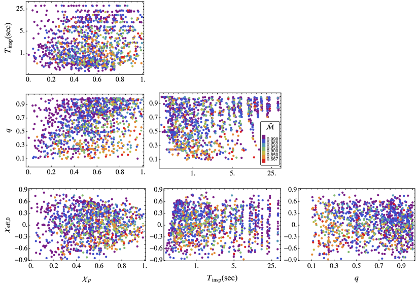
Figure 12: Similar to Figs. 6 and 8, but now for matches at an inclination of $\iota_{s}=\pi/3$ between TEOBResumSP and SEOBNRv4PHM for the entire set of 1230 cases. We have also added the inspiral time, $T_{\text{insp}}$ (note the log scale) to the plots. As written in Sec. IV.4, the matches degrade for low values of $q$, more negative values of $\chi_{\text{eff},0}$, and increasing values of $\chi_{p}$ (or $\chi_{\perp,\text{max}}$). The corresponding figures for $\iota_{s}=0,\pi/6$ are similar, albeit with fewer red and orange dots, and more purple dots.

One way to do this is as in Ref. Babak et al. (2017): by Euler-rotating the inspiralling modes to the $\mathbf{J}_{\text{peak}}$ frame to attach the ringdown portion of the modes, where $\mathbf{J}_{\text{peak}}$ is extracted from the solutions to the precession ODEs at a certain peak. The stitched inspiral-merger-ringdown GW modes are then rotated to the desired inertial frame. It seems, however, that these steps might be redundant as SEOBNRv4PHM successfully stitches the inspiral-merger-ringdown portions in the co-precessing frame Ossokine et al. (2020). See the end of Sec. III for a more detailed discussion.

The next task, after the incorporation of merger-ringdown, is to add higher ($\ell\geq 3$) modes to TEOBResumSP. As Ref. Nagar et al. (2020) states, the non-precessing TEOBResumS $(3,\pm 3),(3,\pm 2),(4,\pm 4)$, and $(5,\pm 5)$ modes show excellent agreement with NR results, so they can be twisted then added to the strain. Thus, in principle, TEOBResumSP can extend up to $\ell=5$, albeit in an incomplete manner, but SEOBNRv4PHM also only has these modes [no $(3,\pm 2)$] and has shown improved agreement as compared to its ($\ell=2$)-only version Ossokine et al. (2020).

Another planned improvement is to couple the precession equations to the TEOBResumS dynamics. This will enable us to generate aligned-spin waveforms with time-varying $\chi_{1}=\mathbf{S}_{1}(t)\cdot\mathbf{L}_{\text{N}}(t)/m_{1}^{2},\chi_{2}=\mathbf{S}_{2}(t)\cdot\mathbf{L}_{\text{N}}(t)/m_{2}^{2}$. This upgrade might improve TEOBResumSP’s agreement with NRSur7dq4 and SEOBNRv4PHM for the strongly precessing cases. Finally, we will test whether or not replacing the SpinTaylorT4 expression for $\dot{v}$ with one obtained from the aligned-spin TEOBResumS dynamics may further improve TEOBResumSP’s performance.

As it stands, the current version of TEOBResumSP yields values greater than $0.965$ for $91\%,86\%,77\%$ of the matches with NRSur7dq4, SEOBNRv4PHM, and IMRPhenomPv3HM respectively. The significantly disagreeing cases either have very strong precession, small mass ratios or rather negative spins. A nice feature of TEOBResumSP is that it is fast thanks to the post-adiabatic method implemented in TEOBResumS which “rushes” the inspiral Nagar and Rettegno (2019).  We expect that, with the above additions, TEOBResumSP will become another useful precessing approximant for the analysis of future GW events. TEOBResumSP will be added to the TEOBResumS git repository https://bitbucket.org/eob_ihes/teobresums/wiki/Home.

Appendix A Derivation of the post-Newtonian spin precession equations up to N4LO

This section builds upon the work of Ref. Sturani . Recall that the $\dot{\hat{\,\mathbf{L}}}_{\text{N}}$ equation is obtained by imposing total angular momentum conservation, $\dot{\mathbf{J}}=0$ which leads to

$$\dot{\mathbf{\,L}}=-\dot{\mathbf{S}}_{1}-\dot{\mathbf{S}}_{2}.$$ (27)

$\mathbf{L}$ is provided up to 3.5 PN in, e.g., Eq. (4.7) of Ref. Bohe et al. (2013) which we rewrite in the following compact form

$$\mathbf{L} =\frac{\eta}{v}\left\{\!\hat{\,\mathbf{L}}_{\text{N}}\left[1+v^{2}\left(\frac{3}{2}+\frac{\eta}{6}\right)\right.\right.$$

$$\hskip 54.06023pt\left.\,+v^{4}\left(\frac{27}{8}-\frac{19\eta}{8}+\frac{\eta^{2}}{24}\right)+\mathcal{O}(v^{6})\right]$$

$$\hskip 31.29802pt+v^{3}\Delta\mathbf{L}_{1.5\text{PN}}^{S}+v^{5}\Delta\mathbf{L}_{2.5\text{PN}}^{S}+v^{7}\Delta\mathbf{L}_{3.5\text{PN}}^{S}$$

$$\hskip 22.76219pt\left.{\color[rgb]{1,1,1}\frac{1}{2}}+\mathcal{O}(v^{8})\right\},$$ (28)

where we defined the terms $\Delta\mathbf{L}_{n\text{PN}}^{S}$ with $n=1.5,2.5,3.5$ with their explicit $v$ scalings factored out. From Ref. Bohe et al. (2013), we can extract

$$\Delta\mathbf{L}_{1.5\text{PN}}^{S} ={\bm{\ell}}\left(-\frac{35}{6}S_{\ell}-\frac{5}{2}\delta m\,\Sigma_{\ell}\right)$$ (29)

$$-{\bm{\lambda}}\left(3S_{\lambda}+\delta m\,\Sigma_{\lambda}\right)+{\mathbf{n}}\left(\frac{1}{2}S_{n}+\frac{1}{2}\delta m\,\Sigma_{n}\right),$$

where ${\bm{\ell}}=\!\hat{\,\mathbf{L}}_{\text{N}}$, ${\bm{n}}=\mathbf{r}/|\mathbf{r}|$ is the relative separation unit vector, and ${\bm{\lambda}}={\bm{\ell}}\times{\bm{n}}$. Moreover, $S_{\ell,\lambda,n}\equiv\{{\bm{\ell}},{\bm{\lambda}},{\bm{n}}\}\cdot\mathbf{S},\Sigma_{\ell,\lambda,n}\equiv\{{\bm{\ell}},{\bm{\lambda}},{\bm{n}}\}\cdot\bm{\Sigma}$, where $\mathbf{S}=\mathbf{S}_{1}+\mathbf{S}_{2},\bm{\Sigma}=\mathbf{S}_{2}/m_{2}-\mathbf{S}_{1}/m_{1}$. Defining $\mathbf{S}_{1\ell}\equiv{\bm{\ell}}({\bm{\ell}}\cdot\mathbf{S}_{1})$ and similarly for $\mathbf{S}_{1\lambda},\mathbf{S}_{1n}$ as well as the $1\to 2$ counterparts, Eq. (29) becomes

$$\Delta\mathbf{L}_{1.5\text{PN}}^{S}= -\frac{5}{6m_{1}}(3M+m_{1})\mathbf{S}_{1\ell}+\frac{(M-m_{1})}{2m_{1}}\mathbf{S}_{1n}$$

$$-\frac{(M+m_{1})}{m_{1}}\mathbf{S}_{1\lambda}+(1\to 2),$$ (30)

where we restored $M=m_{1}+m_{2}$ for clarity in this section. We can now orbit-average this expression using $\langle\hat{n}^{i}\hat{n}^{j}\rangle=\langle\hat{\lambda}^{i}\hat{\lambda}^{j}\rangle=\tfrac{1}{2}(\delta^{ij}-\hat{\ell}^{i}\hat{\ell}^{j})$ which yields $\langle\mathbf{S}_{1n}\rangle=\langle\mathbf{S}_{1\lambda}\rangle=\tfrac{1}{2}(\mathbf{S}_{1}-\mathbf{S}_{1\ell})$. Substituting these orbit-average terms into Eq. (30) we arrive at

$$\Delta\mathbf{L}_{1.5\text{PN}}^{S}= -\frac{M+3m_{1}}{4m_{1}}\mathbf{S}_{1}-\frac{(27M+m_{1})}{12m_{1}}\!\hat{\,\mathbf{L}}_{\text{N}}(\!\hat{\,\mathbf{L}}_{\text{N}}\cdot\mathbf{S}_{1})$$

$$+(1\to 2).$$ (31)

Similarly, with some more determination, one can obtain

$$\Delta\mathbf{L}_{2.5\text{PN}}^{S}=\left(\frac{7M-31m_{1}}{16m_{1}}+\eta\frac{22M+9m_{1}}{48m_{1}}\right)\mathbf{S}_{1}$$

$$+\left[-\frac{49M+39m_{1}}{16m_{1}}+\eta\left(\frac{59M}{24m_{1}}-\frac{13}{144}\right)\right]\!\hat{\,\mathbf{L}}_{\text{N}}(\!\hat{\,\mathbf{L}}_{\text{N}}\cdot\mathbf{S}_{1})$$

$$+(1\to 2).$$ (32)

Eq. (29) inside Eq. (28) together with Eqs. (4a, 4b) give us all the pieces that we need to go to N4LO [Eq. (32) enters at N5LO so we drop it.] For clarity, let us once again consider NNLO first. At this order, Eq. (28) becomes

$$\mathbf{L}= \!\hat{\,\mathbf{L}}_{\text{N}}\,\frac{\eta}{v}\text{L}_{1\text{PN}}+\eta v^{2}\left(c_{S1}\mathbf{S}_{1}+c_{S2}\mathbf{S}_{2}\right)$$

$$+ \eta v^{2}\!\hat{\,\mathbf{L}}_{\text{N}}\left(c_{S1L}\!\hat{\,\mathbf{L}}_{\text{N}}\cdot\mathbf{S}_{1}+c_{S2L}\!\hat{\,\mathbf{L}}_{\text{N}}\cdot\mathbf{S}_{2}\right),$$ (33)

where $\text{L}_{1\text{PN}}\equiv 1+v^{2}\left(\tfrac{3}{2}+\tfrac{1}{6}\eta\right)$ and the constants $c_{S1},c_{S1L}$, etc., are given in Eqs. (6a, 6b). Differentiating Eq. (33) with respect to time, we obtain

$$\dot{\hat{\,\mathbf{L}}}_{\text{N}}^{\text{NNLO}}=\frac{v}{\eta}\frac{1}{\text{L}_{1\text{PN}}} \left[-\dot{\mathbf{S}}_{1}^{\text{NNLO}}-\dot{\mathbf{S}}_{2}^{\text{NNLO}}\right.$$

$$\left.-\eta v^{2}\left(c_{S1}\dot{\mathbf{S}}_{1}^{\text{LO}}+c_{S2}\dot{\mathbf{S}}_{2}^{\text{LO}}\right)\right],$$ (34)

where, e.g., $\dot{\mathbf{S}}_{1}^{\text{NNLO}}$ implies that only terms that scale as $v^{\leq 7}$ should be retained. Several simplifications occurred in reaching Eq. (34). First, the second $\dot{\mathbf{S}}_{1},\dot{\mathbf{S}}_{2}$ terms contribute only at the LO. This is because of the factor of $v^{2}$ in front, which means that at our required order, i.e., NNLO, the terms multiplying $v^{2}$ can be at most $\propto v^{5}$ which is LO for $\dot{\mathbf{S}}_{1},\dot{\mathbf{S}}_{2}$ as can be seen from Eqs. (1a, 1b). Second, all the $c_{S1L},c_{S2L}$ terms have dropped from Eq. (34) because (i) $v^{2}\dot{\hat{\,\mathbf{L}}}_{\text{N}}\propto v^{8}$, i.e., is N3LO and (ii) at NNLO only $v^{2}\!\hat{\,\mathbf{L}}_{\text{N}}\cdot\dot{\mathbf{S}}_{1}^{\text{LO}}$ scales as $v^{7}$, but is actually zero because $\!\hat{\,\mathbf{L}}_{\text{N}}\perp\dot{\mathbf{S}}_{1}^{\text{LO}}$ as is clear from Eqs. (1a, 1b).

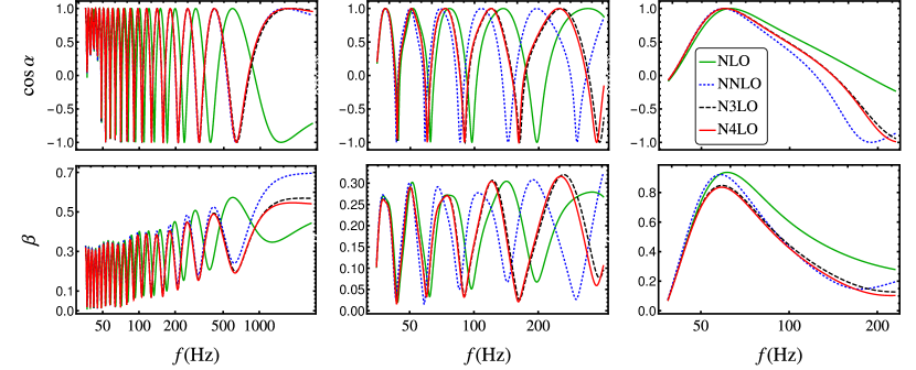
Figure 13: The spherical angles of $\mathbf{L}_{\text{N}}(t)$ in the $\mathbf{L}_{0}$ frame described in Sec. II.2 for three separate cases: binary neutron star (left panels), black hole neutron star (middle panels), and binary black hole (right panels) inspirals. $\alpha$ is the azimuthal angle and $\beta$ is the polar angle (see Fig. 1). In each panel, we show the angle obtained from solving the precession ODEs truncated at four different orders: NLO, NNLO, N3LO, and N4LO. From left to right, the binaries respectively have $M=3,20,35M_{\odot}$, $q\approx 0.85,0.11,0.35$, and $\chi_{p}\approx 0.78,0.22,0.74$. $f$ represents the (2,2)-mode gravitational wave frequency.

Pushing now to N4LO, Eq. (27) becomes

$$\dot{\mathbf{\,L}} =\dot{\hat{\,\mathbf{L}}}_{\text{N}}\frac{\eta}{v}\text{L}_{2\text{PN}}+\eta v^{2}\dot{\Delta\mathbf{L}}^{S}_{1.5\text{PN}}=-\dot{\mathbf{S}}_{1}^{\text{N4LO}}-\dot{\mathbf{S}}_{2}^{\text{N4LO}},$$ (35)

where $\text{L}_{2\text{PN}}$ is given in Eq. (5b). Note that we omit the radiation reaction terms starting at NNLO via $\eta\dot{v}/v^{2}\propto v^{7}$ in $\dot{\mathbf{\,L}}$ because they drop out from $\dot{\hat{\,\mathbf{L}}}_{\text{N},\perp}$ given in Eq. (7) since these terms are all parallel to $\!\hat{\,\mathbf{L}}_{\text{N}}$. The effects of radiation reaction are incorporated via $v=v(t)$ in the precession ODEs after the standard change of variables $d/dt\to\dot{v}(v)d/dv$ in Eqs. (1a) - (5a).

Explicitly writing out Eq. (35) at N4LO then rearranging gives us Eq. (4c), where we used the property that $\dot{\mathbf{S}}_{i}\perp\mathbf{S}_{i}$ up to NLO. In terms of powers of $v$, each term in Eq. (4c) goes up to $v^{9}$, i.e., N4LO as defined.

We can now obtain $\mathbf{L}_{\text{N}}$, therefore, the angles $\alpha$ and $\beta$ at any order of our choosing varying from NLO to N4LO, which we show in Fig. 13 as functions of the (2,2)-mode GW frequency for three different precessing compact binary inspirals. As can be seen in the figure, the angles from different orders remain very close to each other in general until the binaries enter their respective strong-gravity regimes. The angle dephasing between different orders happens earlier and is most prominent for the most asymmetric system in the figure, i.e., a black hole neutron star binary with $M=20M_{\odot}$ and $q\approx 0.11$. The differences between the N3LO and N4LO angles are much smaller, expectedly so since the differences of these two orders scales as $v^{9}$.

A thorough survey of the effects of the truncation order of the precession ODEs, the instantaneous terms (entering at N3LO), and the neglected terms would be beneficial to the entire gravitational-wave community. Ref. Ossokine et al. (2015) has already done some work in this regard, but a systematic, large-scale analysis quantified in terms of consequences to parameter estimation remains to be undertaken at this point.

Appendix B Results of using NLO angles and a different twist formula

In this section, we briefly show results from two additional test we conducted: (1) Using Euler angles in the twist formula (20) that are obtained from the precession ODEs truncated at NLO as given in Eqs. (1a)-(1c). (2) Using N4LO Euler angles in an alternate twist formula. Specifically, we have chosen to test the expression provided by Eq. (A2) of Ref. Khan et al. (2019b)

$$h_{\ell m}^{\text{T}}(t)=e^{im\alpha}\sum_{m^{\prime}=-l}^{l}e^{-im^{\prime}\gamma}d^{\ell}_{m^{\prime},m}(-\beta)\,h_{lm^{\prime}}^{\text{NP}}\,.$$ (36)

This version differs from our twist formula (20) in the signs of the $\alpha$ and $\gamma$ exponents. For convenience, we redisplay our expression

$$h_{\ell m}^{\text{T}}(t)=e^{-im\alpha}\sum_{m^{\prime}=-l}^{l}e^{im^{\prime}\gamma}d^{\ell}_{m^{\prime},m}(-\beta)\,h_{lm^{\prime}}^{\text{NP}}\,.$$ (37)

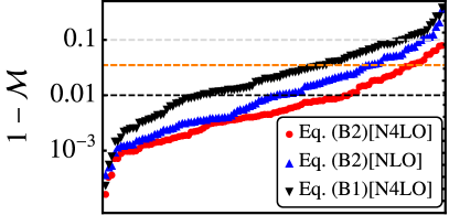
Figure 14: Performance of two alternate TEOBResumS twists against our standard twist measured in terms of $\ell=2$ detector strain mismatches with NRSur7dq4 (50 cases) and SEOBNRv4PHM (60 cases) ordered by increasing mismatch. Red circles represent mismatches obtained using our standard expression, dubbed Eq. (37)[N4LO]: twisting via Eq. (37) with angles obtained from the precession ODEs truncated at N4LO. Similarly, the blue triangles represent mismatches obtained with the same twist formula, but with angles coming from the NLO-truncated ODEs, hence dubbed Eq. (37)[NLO]. Finally, the inverted black triangles represent mismatches resulting from using the alternate twist formula (36) at N4LO. As before, the horizontal dashed black, orange, and gray lines mark ${\cal M}=0.99,0.965,0.9$. It is clear from the figure that our standard expression produces the best matches. We left the horizontal axis unlabelled since we reordered the total of 110 cases in terms of increasing $1-{\cal M}$.

For both tests, we used a subset of precessing compact binary inspirals that is a combination of 50 cases from our NRSur7dq4 set and 60 cases from our SEOBNRv4PHM set. Using Eq. (36) at N4LO and Eq. (37) at NLO we generated two new sets of twisted $\ell=2$ TEOBResumS modes with which we then computed the $\ell=2$ detector strain matches as before. We show how these two alternate twists perform against ours, dubbed Eq. (37)[N4LO], in Fig. 14, where it is evident that our twist produces consistently the smallest mismatches (red circles). The alternate twist formula of Eq. (36) is clearly the worst choice producing ${\cal M}>0.965$ for only about two thirds of the set (black inverted triangles). The reason why Eq. (36)[N4LO] still somehow manages to mostly yield ${\cal M}>0.965$ is due to both the fact that $\gamma$ remains close to $\alpha$ because $\beta$, starting from zero, is small for most binaries, and that the twisted $(2,\pm 2)$ modes differ by a small amount. Therefore, in binaries for which $\beta(t)\ll 1$ and the precessing $(2,\pm 2)$ modes dominate the mode-sum in the strain formula (23), Eqs. (36) and (37) are nearly equal under the $m\to-m$ exchange, thus produce twisted waveform strains that are very close to each other.

Returning to Fig. 14, we see that the NLO version of our twist performs somewhat well in the sense that roughly three quarters of the cases yielded ${\cal M}>0.965$ (blue triangles). The details of the differences in the plotted NLO, N4LO mismatches lay with the differences in the Euler angles used in the respective twists. We have already shown in Fig. 13 how these Euler angles vary as the ODE truncation order goes from NLO to N4LO. For most cases, the difference in the angles become significant only in the last few orbital cycles, corresponding to the small differences between the NLO and N4LO mismatches of Fig. 14. But for cases with small $q$, the differences in the Euler angles becomes more significant as can be seen in the middle panels of Fig. 13. It is possible that the speed-up gained in using NLO-truncated precession ODEs, instead of N4LO, is significant enough to justify their use in parameter estimation. As we have not yet carried out detailed speed tests of our code, we can not verify or refute this hypothesis, but will do so with the next version of TEOBResumSP.

References

- Aasi et al. (2015) J. Aasi et al. (LIGO Scientific), Class. Quant. Grav. 32, 074001 (2015), arXiv:1411.4547 [gr-qc] .
- Acernese et al. (2015) F. Acernese et al. (VIRGO), Class. Quant. Grav. 32, 024001 (2015), arXiv:1408.3978 [gr-qc] .
- Abbott et al. (2016a) B. P. Abbott et al. (Virgo, LIGO Scientific), Phys. Rev. Lett. 116, 061102 (2016a), arXiv:1602.03837 [gr-qc] .
- Abbott et al. (2017a) B. P. Abbott et al. (Virgo, LIGO Scientific), Phys. Rev. Lett. 119, 161101 (2017a), arXiv:1710.05832 [gr-qc] .
- Abbott et al. (2016b) B. P. Abbott et al. (Virgo, LIGO Scientific), Phys. Rev. Lett. 116, 241103 (2016b), arXiv:1606.04855 [gr-qc] .
- Abbott et al. (2017b) B. P. Abbott et al. (Virgo, LIGO Scientific), Astrophys. J. 851, L35 (2017b), arXiv:1711.05578 [astro-ph.HE] .
- Abbott et al. (2017c) B. P. Abbott et al. (Virgo, LIGO Scientific), Phys. Rev. Lett. 119, 141101 (2017c), arXiv:1709.09660 [gr-qc] .
- Abbott et al. (2017d) B. P. Abbott et al. (VIRGO, LIGO Scientific), Phys. Rev. Lett. 118, 221101 (2017d), arXiv:1706.01812 [gr-qc] .
- Abbott et al. (2019a) B. P. Abbott et al. (LIGO Scientific, Virgo), Phys. Rev. X9, 031040 (2019a), arXiv:1811.12907 [astro-ph.HE] .
- Venumadhav et al. (2019) T. Venumadhav, B. Zackay, J. Roulet, L. Dai, and M. Zaldarriaga, Phys. Rev. D 100, 023011 (2019), arXiv:1902.10341 [astro-ph.IM] .
- Venumadhav et al. (2020) T. Venumadhav, B. Zackay, J. Roulet, L. Dai, and M. Zaldarriaga, Phys. Rev. D 101, 083030 (2020), arXiv:1904.07214 [astro-ph.HE] .
- Nitz et al. (2019) A. H. Nitz, C. Capano, A. B. Nielsen, S. Reyes, R. White, D. A. Brown, and B. Krishnan, Astrophys. J. 872, 195 (2019), arXiv:1811.01921 [gr-qc] .
- Nitz et al. (2020) A. H. Nitz, T. Dent, G. S. Davies, S. Kumar, C. D. Capano, I. Harry, S. Mozzon, L. Nuttall, A. Lundgren, and M. Tápai, Astrophys. J. 891, 123 (2020), arXiv:1910.05331 [astro-ph.HE] .
- Abbott et al. (2020a) B. Abbott et al. (LIGO Scientific, Virgo), Astrophys. J. Lett. 892, L3 (2020a), arXiv:2001.01761 [astro-ph.HE] .
- Abbott et al. (2020b) R. Abbott et al. (LIGO Scientific, Virgo), Phys. Rev. D 102, 043015 (2020b), arXiv:2004.08342 [astro-ph.HE] .
- Abbott et al. (2020c) R. Abbott et al. (LIGO Scientific, Virgo), Astrophys. J. Lett. 896, L44 (2020c), arXiv:2006.12611 [astro-ph.HE] .
- Abbott et al. (2020d) R. Abbott et al. (LIGO Scientific, Virgo), Phys. Rev. Lett. 125, 101102 (2020d), arXiv:2009.01075 [gr-qc] .
- (18) “GraceDB — Gravitational-Wave Candidate Event Database,” https://gracedb.ligo.org/superevents/public/O3/.
- Abbott et al. (2020e) R. Abbott et al., (2020e), arXiv:2010.14527 [gr-qc] .
- Blanchet (2014) L. Blanchet, Living Rev. Relativity 17, 2 (2014), arXiv:1310.1528 [gr-qc] .
- Gourgoulhon (2012) E. Gourgoulhon, 3+1 formalism and bases of numerical relativity, Lecture notes in physics (Springer, Berlin, 2012) arXiv:gr-qc/0703035 [GR-QC] .
- Centrella et al. (2010) J. Centrella, J. G. Baker, B. J. Kelly, and J. R. van Meter, Rev. Mod. Phys. 82, 3069 (2010), arXiv:1010.5260 [gr-qc] .
- Buonanno and Damour (1999) A. Buonanno and T. Damour, Phys. Rev. D59, 084006 (1999), arXiv:gr-qc/9811091 .
- Buonanno and Damour (2000) A. Buonanno and T. Damour, Phys. Rev. D62, 064015 (2000), arXiv:gr-qc/0001013 .
- Ajith et al. (2007) P. Ajith, S. Babak, Y. Chen, M. Hewitson, B. Krishnan, et al., Class.Quant.Grav. 24, S689 (2007), arXiv:0704.3764 [gr-qc] .
- Ajith et al. (2008) P. Ajith, S. Babak, Y. Chen, M. Hewitson, B. Krishnan, et al., Phys.Rev. D77, 104017 (2008), arXiv:0710.2335 [gr-qc] .
- Bernard et al. (2018) L. Bernard, L. Blanchet, G. Faye, and T. Marchand, Phys. Rev. D97, 044037 (2018), arXiv:1711.00283 [gr-qc] .
- Messina et al. (2019) F. Messina, R. Dudi, A. Nagar, and S. Bernuzzi, Phys. Rev. D99, 124051 (2019), arXiv:1904.09558 [gr-qc] .
- Buonanno et al. (2009) A. Buonanno, B. Iyer, E. Ochsner, Y. Pan, and B. Sathyaprakash, Phys.Rev. D80, 084043 (2009), arXiv:0907.0700 [gr-qc] .
- Damour et al. (2012) T. Damour, A. Nagar, and L. Villain, Phys.Rev. D85, 123007 (2012), arXiv:1203.4352 [gr-qc] .
- Sturani et al. (2010) R. Sturani, S. Fischetti, L. Cadonati, G. Guidi, J. Healy, et al., J.Phys.Conf.Ser. 243, 012007 (2010), arXiv:1005.0551 [gr-qc] .
- Pretorius (2005) F. Pretorius, Phys. Rev. Lett. 95, 121101 (2005), arXiv:gr-qc/0507014 .
- Campanelli et al. (2006) M. Campanelli, C. O. Lousto, P. Marronetti, and Y. Zlochower, Phys. Rev. Lett. 96, 111101 (2006), arXiv:gr-qc/0511048 .
- Baker et al. (2006) J. G. Baker, J. Centrella, D.-I. Choi, M. Koppitz, and J. van Meter, Phys. Rev. Lett. 96, 111102 (2006), arXiv:gr-qc/0511103 .
- Mroue et al. (2013) A. H. Mroue, M. A. Scheel, B. Szilagyi, H. P. Pfeiffer, M. Boyle, et al., Phys.Rev.Lett. 111, 241104 (2013), arXiv:1304.6077 [gr-qc] .
- Boyle et al. (2019) M. Boyle et al., Class. Quant. Grav. 36, 195006 (2019), arXiv:1904.04831 [gr-qc] .
- (37) “SXS Gravitational Waveform Database,” https://data.black-holes.org/waveforms/index.html.
- Jani et al. (2016) K. Jani, J. Healy, J. A. Clark, L. London, P. Laguna, and D. Shoemaker, Class. Quant. Grav. 33, 204001 (2016), arXiv:1605.03204 [gr-qc] .
- (39) “Georgia Tech catalog of binary black hole simulations,” http://www.einstein.gatech.edu/catalog/.
- (40) “CCRG@RIT Catalog of Numerical Simulations,” https://ccrg.rit.edu/numerical-simulations.
- Healy et al. (2017) J. Healy, C. O. Lousto, Y. Zlochower, and M. Campanelli, Class. Quant. Grav. 34, 224001 (2017), arXiv:1703.03423 [gr-qc] .
- Dietrich et al. (2018) T. Dietrich, D. Radice, S. Bernuzzi, F. Zappa, A. Perego, B. Brügmann, S. V. Chaurasia, R. Dudi, W. Tichy, and M. Ujevic, Class. Quant. Grav. 35, 24LT01 (2018), arXiv:1806.01625 [gr-qc] .
- (43) “CoRe: Computational Relativity,” http://www.computational-relativity.org/.
- Ajith et al. (2011) P. Ajith, M. Hannam, S. Husa, Y. Chen, B. Brügmann, et al., Phys.Rev.Lett. 106, 241101 (2011), arXiv:0909.2867 [gr-qc] .
- Santamaria et al. (2010) L. Santamaria, F. Ohme, P. Ajith, B. Brügmann, N. Dorband, et al., Phys.Rev. D82, 064016 (2010), arXiv:1005.3306 [gr-qc] .
- Husa et al. (2016) S. Husa, S. Khan, M. Hannam, M. Pürrer, F. Ohme, X. Jiménez Forteza, and A. Bohé, Phys. Rev. D93, 044006 (2016), arXiv:1508.07250 [gr-qc] .
- Khan et al. (2016) S. Khan, S. Husa, M. Hannam, F. Ohme, M. Pürrer, X. Jiménez Forteza, and A. Bohé, Phys. Rev. D93, 044007 (2016), arXiv:1508.07253 [gr-qc] .
- Dietrich et al. (2017) T. Dietrich, S. Bernuzzi, and W. Tichy, Phys. Rev. D96, 121501 (2017), arXiv:1706.02969 [gr-qc] .
- Dietrich et al. (2019a) T. Dietrich, A. Samajdar, S. Khan, N. K. Johnson-McDaniel, R. Dudi, and W. Tichy, Phys. Rev. D100, 044003 (2019a), arXiv:1905.06011 [gr-qc] .
- London et al. (2018) L. London, S. Khan, E. Fauchon-Jones, X. J. Forteza, M. Hannam, S. Husa, C. Kalaghatgi, F. Ohme, and F. Pannarale, Phys. Rev. Lett. 120, 161102 (2018), arXiv:1708.00404 [gr-qc] .
- Hannam et al. (2014) M. Hannam, P. Schmidt, A. Bohé, L. Haegel, S. Husa, F. Ohme, G. Pratten, and M. Pürrer, Phys. Rev. Lett. 113, 151101 (2014), arXiv:1308.3271 [gr-qc] .
- Schmidt et al. (2015) P. Schmidt, F. Ohme, and M. Hannam, Phys. Rev. D91, 024043 (2015), arXiv:1408.1810 [gr-qc] .
- Pratten et al. (2020a) G. Pratten, S. Husa, C. Garcia-Quiros, M. Colleoni, A. Ramos-Buades, H. Estelles, and R. Jaume, Phys. Rev. D 102, 064001 (2020a), arXiv:2001.11412 [gr-qc] .
- García-Quirós et al. (2020a) C. García-Quirós, M. Colleoni, S. Husa, H. Estellés, G. Pratten, A. Ramos-Buades, M. Mateu-Lucena, and R. Jaume, Phys. Rev. D 102, 064002 (2020a), arXiv:2001.10914 [gr-qc] .
- García-Quirós et al. (2020b) C. García-Quirós, S. Husa, M. Mateu-Lucena, and A. Borchers, (2020b), arXiv:2001.10897 [gr-qc] .
- Chatziioannou et al. (2017) K. Chatziioannou, A. Klein, N. Yunes, and N. Cornish, Phys. Rev. D95, 104004 (2017), arXiv:1703.03967 [gr-qc] .
- Khan et al. (2019a) S. Khan, K. Chatziioannou, M. Hannam, and F. Ohme, Phys. Rev. D100, 024059 (2019a), arXiv:1809.10113 [gr-qc] .
- Khan et al. (2019b) S. Khan, F. Ohme, K. Chatziioannou, and M. Hannam, (2019b), arXiv:1911.06050 [gr-qc] .
- Pratten et al. (2020b) G. Pratten et al., (2020b), arXiv:2004.06503 [gr-qc] .
- Estellés et al. (2020) H. Estellés, A. Ramos-Buades, S. Husa, C. García-Quirós, M. Colleoni, L. Haegel, and R. Jaume, (2020), arXiv:2004.08302 [gr-qc] .
- Damour and Nagar (2009) T. Damour and A. Nagar, Phys. Rev. D79, 081503 (2009), arXiv:0902.0136 [gr-qc] .
- Damour and Nagar (2014a) T. Damour and A. Nagar, Phys.Rev. D90, 044018 (2014a), arXiv:1406.6913 [gr-qc] .
- Damour et al. (2009) T. Damour, B. R. Iyer, and A. Nagar, Phys. Rev. D79, 064004 (2009), arXiv:0811.2069 [gr-qc] .
- Pan et al. (2011) Y. Pan, A. Buonanno, R. Fujita, E. Racine, and H. Tagoshi, Phys.Rev. D83, 064003 (2011), arXiv:1006.0431 [gr-qc] .
- Damour and Nagar (2014b) T. Damour and A. Nagar, Phys.Rev. D90, 024054 (2014b), arXiv:1406.0401 [gr-qc] .
- Bohé et al. (2017) A. Bohé et al., Phys. Rev. D95, 044028 (2017), arXiv:1611.03703 [gr-qc] .
- Nagar et al. (2017) A. Nagar, G. Riemenschneider, and G. Pratten, Phys. Rev. D96, 084045 (2017), arXiv:1703.06814 [gr-qc] .
- Pürrer (2014) M. Pürrer, Class. Quant. Grav. 31, 195010 (2014), arXiv:1402.4146 [gr-qc] .
- Babak et al. (2017) S. Babak, A. Taracchini, and A. Buonanno, Phys. Rev. D95, 024010 (2017), arXiv:1607.05661 [gr-qc] .
- Cotesta et al. (2018) R. Cotesta, A. Buonanno, A. Bohé, A. Taracchini, I. Hinder, and S. Ossokine, Phys. Rev. D98, 084028 (2018), arXiv:1803.10701 [gr-qc] .
- Nagar et al. (2018) A. Nagar et al., Phys. Rev. D98, 104052 (2018), arXiv:1806.01772 [gr-qc] .
- Damour and Nagar (2010) T. Damour and A. Nagar, Phys. Rev. D81, 084016 (2010), arXiv:0911.5041 [gr-qc] .
- Bernuzzi et al. (2012) S. Bernuzzi, A. Nagar, M. Thierfelder, and B. Brügmann, Phys.Rev. D86, 044030 (2012), arXiv:1205.3403 [gr-qc] .
- Lackey et al. (2014) B. D. Lackey, K. Kyutoku, M. Shibata, P. R. Brady, and J. L. Friedman, Phys.Rev. D89, 043009 (2014), arXiv:1303.6298 [gr-qc] .
- Bernuzzi et al. (2015) S. Bernuzzi, A. Nagar, T. Dietrich, and T. Damour, Phys.Rev.Lett. 114, 161103 (2015), arXiv:1412.4553 [gr-qc] .
- Hinderer et al. (2016) T. Hinderer et al., Phys. Rev. Lett. 116, 181101 (2016), arXiv:1602.00599 [gr-qc] .
- Steinhoff et al. (2016) J. Steinhoff, T. Hinderer, A. Buonanno, and A. Taracchini, Phys. Rev. D94, 104028 (2016), arXiv:1608.01907 [gr-qc] .
- Dietrich et al. (2019b) T. Dietrich et al., Phys. Rev. D99, 024029 (2019b), arXiv:1804.02235 [gr-qc] .
- Akcay et al. (2019) S. Akcay, S. Bernuzzi, F. Messina, A. Nagar, N. Ortiz, and P. Rettegno, Phys. Rev. D99, 044051 (2019), arXiv:1812.02744 [gr-qc] .
- Lackey et al. (2019) B. D. Lackey, M. Pürrer, A. Taracchini, and S. Marsat, Phys. Rev. D 100, 024002 (2019), arXiv:1812.08643 [gr-qc] .
- Matas et al. (2020) A. Matas et al., (2020), arXiv:2004.10001 [gr-qc] .
- Thompson et al. (2020) J. E. Thompson, E. Fauchon-Jones, S. Khan, E. Nitoglia, F. Pannarale, T. Dietrich, and M. Hannam, Phys. Rev. D 101, 124059 (2020), arXiv:2002.08383 [gr-qc] .
- Vines et al. (2011) J. Vines, E. E. Flanagan, and T. Hinderer, Phys. Rev. D83, 084051 (2011), arXiv:1101.1673 [gr-qc] .
- Henry et al. (2020) Q. Henry, G. Faye, and L. Blanchet, Phys. Rev. D 102, 044033 (2020), arXiv:2005.13367 [gr-qc] .
- Abbott et al. (2019b) B. P. Abbott et al. (LIGO Scientific, Virgo), (2019b), arXiv:1903.04467 [gr-qc] .
- Chatziioannou et al. (2019) K. Chatziioannou et al., Phys. Rev. D100, 104015 (2019), arXiv:1903.06742 [gr-qc] .
- Mandel and Fragos (2020) I. Mandel and T. Fragos, (2020), arXiv:2004.09288 [astro-ph.HE] .
- Abbott et al. (2020f) R. Abbott et al. (LIGO Scientific, Virgo), Astrophys. J. Lett. 900, L13 (2020f), arXiv:2009.01190 [astro-ph.HE] .
- Apostolatos et al. (1994) T. A. Apostolatos, C. Cutler, G. J. Sussman, and K. S. Thorne, Phys. Rev. D49, 6274 (1994).
- Pürrer and Haster (2020) M. Pürrer and C.-J. Haster, Phys. Rev. Res. 2, 023151 (2020), arXiv:1912.10055 [gr-qc] .
- Harry et al. (2016) I. Harry, S. Privitera, A. Bohé, and A. Buonanno, Phys. Rev. D94, 024012 (2016), arXiv:1603.02444 [gr-qc] .
- Calderón Bustillo et al. (2017) J. Calderón Bustillo, P. Laguna, and D. Shoemaker, Phys. Rev. D95, 104038 (2017), arXiv:1612.02340 [gr-qc] .
- Barker and O’Connell (1979) B. M. Barker and R. F. O’Connell, Gen. Rel. Grav. 11, 149 (1979).
- Thorne and Hartle (1984) K. S. Thorne and J. B. Hartle, Phys. Rev. D31, 1815 (1984).
- Mathisson (1937) M. Mathisson, Acta Phys. Polon. 6, 163 (1937).
- Papapetrou (1951) A. Papapetrou, Proc. Roy. Soc. Lond. A209, 248 (1951).
- Dixon (1970) W. G. Dixon, Proc. Roy. Soc. Lond. A314, 499 (1970).
- LIGO Scientific Collaboration (2018) LIGO Scientific Collaboration, “LIGO Algorithm Library - LALSuite,” free software (GPL) (2018).
- Arun et al. (2009) K. G. Arun, A. Buonanno, G. Faye, and E. Ochsner, Phys. Rev. D79, 104023 (2009), [Erratum: Phys. Rev.D84,049901(2011)], arXiv:0810.5336 [gr-qc] .
- Pan et al. (2014a) Y. Pan, A. Buonanno, A. Taracchini, M. Boyle, L. E. Kidder, et al., Phys.Rev. D89, 061501 (2014a), arXiv:1311.2565 [gr-qc] .
- Ossokine et al. (2020) S. Ossokine et al., (2020), arXiv:2004.09442 [gr-qc] .
- Schmidt et al. (2011) P. Schmidt, M. Hannam, S. Husa, and P. Ajith, Phys. Rev. D84, 024046 (2011), arXiv:1012.2879 [gr-qc] .
- Cutler and Flanagan (1994) C. Cutler and E. E. Flanagan, Phys.Rev. D49, 2658 (1994), arXiv:gr-qc/9402014 [gr-qc] .
- Buonanno et al. (2003) A. Buonanno, Y.-b. Chen, and M. Vallisneri, Phys. Rev. D67, 104025 (2003), [Erratum: Phys. Rev.D74,029904(2006)], arXiv:gr-qc/0211087 [gr-qc] .
- Schmidt et al. (2012) P. Schmidt, M. Hannam, and S. Husa, Phys. Rev. D86, 104063 (2012), arXiv:1207.3088 [gr-qc] .
- Gualtieri et al. (2008) L. Gualtieri, E. Berti, V. Cardoso, and U. Sperhake, Phys. Rev. D 78, 044024 (2008), arXiv:0805.1017 [gr-qc] .
- Campanelli et al. (2009) M. Campanelli, C. O. Lousto, H. Nakano, and Y. Zlochower, Phys. Rev. D79, 084010 (2009), arXiv:0808.0713 [gr-qc] .
- O’Shaughnessy et al. (2011) R. O’Shaughnessy, B. Vaishnav, J. Healy, Z. Meeks, and D. Shoemaker, Phys. Rev. D84, 124002 (2011), arXiv:1109.5224 [gr-qc] .
- Boyle et al. (2011) M. Boyle, R. Owen, and H. P. Pfeiffer, Phys. Rev. D84, 124011 (2011), arXiv:1110.2965 [gr-qc] .
- Field et al. (2011) S. E. Field, C. R. Galley, F. Herrmann, J. S. Hesthaven, E. Ochsner, and M. Tiglio, Phys. Rev. Lett. 106, 221102 (2011), arXiv:1101.3765 [gr-qc] .
- Herrmann et al. (2012) F. Herrmann, S. E. Field, C. R. Galley, E. Ochsner, and M. Tiglio, Phys. Rev. D86, 084046 (2012), arXiv:1205.6009 [gr-qc] .
- Canizares et al. (2013) P. Canizares, S. E. Field, J. R. Gair, and M. Tiglio, Phys. Rev. D87, 124005 (2013), arXiv:1304.0462 [gr-qc] .
- Canizares et al. (2015) P. Canizares, S. E. Field, J. Gair, V. Raymond, R. Smith, and M. Tiglio, Phys. Rev. Lett. 114, 071104 (2015), arXiv:1404.6284 [gr-qc] .
- Pürrer (2016) M. Pürrer, Phys. Rev. D93, 064041 (2016), arXiv:1512.02248 [gr-qc] .
- Doctor et al. (2017) Z. Doctor, B. Farr, D. E. Holz, and M. Pürrer, Phys. Rev. D96, 123011 (2017), arXiv:1706.05408 [astro-ph.HE] .
- Cotesta et al. (2020) R. Cotesta, S. Marsat, and M. Pürrer, Phys. Rev. D 101, 124040 (2020), arXiv:2003.12079 [gr-qc] .
- Blackman et al. (2014) J. Blackman, B. Szilagyi, C. R. Galley, and M. Tiglio, Phys. Rev. Lett. 113, 021101 (2014), arXiv:1401.7038 [gr-qc] .
- Blackman et al. (2017) J. Blackman, S. E. Field, M. A. Scheel, C. R. Galley, D. A. Hemberger, P. Schmidt, and R. Smith, Phys. Rev. D95, 104023 (2017), arXiv:1701.00550 [gr-qc] .
- Varma et al. (2019) V. Varma, S. E. Field, M. A. Scheel, J. Blackman, D. Gerosa, L. C. Stein, L. E. Kidder, and H. P. Pfeiffer, Phys. Rev. Research. 1, 033015 (2019), arXiv:1905.09300 [gr-qc] .
- Williams et al. (2019) D. Williams, I. S. Heng, J. Gair, J. A. Clark, and B. Khamesra, (2019), arXiv:1903.09204 [gr-qc] .
- Fairhurst et al. (2019) S. Fairhurst, R. Green, C. Hoy, M. Hannam, and A. Muir, (2019), arXiv:1908.05707 [gr-qc] .
- Williamson et al. (2017) A. R. Williamson, J. Lange, R. O’Shaughnessy, J. A. Clark, P. Kumar, J. Calderón Bustillo, and J. Veitch, Phys. Rev. D96, 124041 (2017), arXiv:1709.03095 [gr-qc] .
- Nagar et al. (2019a) A. Nagar, F. Messina, P. Rettegno, D. Bini, T. Damour, A. Geralico, S. Akcay, and S. Bernuzzi, Phys. Rev. D99, 044007 (2019a), arXiv:1812.07923 [gr-qc] .
- Nagar and Rettegno (2019) A. Nagar and P. Rettegno, Phys. Rev. D99, 021501 (2019), arXiv:1805.03891 [gr-qc] .
- Nagar et al. (2019b) A. Nagar, G. Pratten, G. Riemenschneider, and R. Gamba, (2019b), arXiv:1904.09550 [gr-qc] .
- Nagar et al. (2020) A. Nagar, G. Riemenschneider, G. Pratten, P. Rettegno, and F. Messina, (2020), arXiv:2001.09082 [gr-qc] .
- Rettegno et al. (2019) P. Rettegno, F. Martinetti, A. Nagar, D. Bini, G. Riemenschneider, and T. Damour, (2019), arXiv:1911.10818 [gr-qc] .
- Bohe et al. (2013) A. Bohe, S. Marsat, G. Faye, and L. Blanchet, Class. Quant. Grav. 30, 075017 (2013), arXiv:1212.5520 [gr-qc] .
- Bohé et al. (2015) A. Bohé, G. Faye, S. Marsat, and E. K. Porter, Class. Quant. Grav. 32, 195010 (2015), arXiv:1501.01529 [gr-qc] .
- Racine et al. (2009) E. Racine, A. Buonanno, and L. E. Kidder, Phys. Rev. D80, 044010 (2009), arXiv:0812.4413 [gr-qc] .
- Kidder (1995) L. E. Kidder, Phys.Rev. D52, 821 (1995), arXiv:gr-qc/9506022 [gr-qc] .
- Pan et al. (2014b) Y. Pan, A. Buonanno, A. Taracchini, L. E. Kidder, A. H. Mroue, et al., Phys.Rev. D89, 084006 (2014b), arXiv:1307.6232 [gr-qc] .
- Chatziioannou et al. (2013) K. Chatziioannou, A. Klein, N. Yunes, and N. Cornish, Phys. Rev. D88, 063011 (2013), arXiv:1307.4418 [gr-qc] .
- (134) R. Sturani, https://dcc.ligo.org/public/0122/T1500554/013/dLdS.pdf.
- Ossokine et al. (2015) S. Ossokine, M. Boyle, L. E. Kidder, H. P. Pfeiffer, M. A. Scheel, and B. Szilágyi, Phys. Rev. D92, 104028 (2015), arXiv:1502.01747 [gr-qc] .
- Ajith (2011) P. Ajith, Phys.Rev. D84, 084037 (2011), arXiv:1107.1267 [gr-qc] .
- Damour (2001) T. Damour, Phys. Rev. D64, 124013 (2001), arXiv:gr-qc/0103018 .
- Racine (2008) E. Racine, Phys. Rev. D78, 044021 (2008), arXiv:0803.1820 [gr-qc] .
- Goldberg et al. (1967) J. N. Goldberg, A. J. MacFarlane, E. T. Newman, F. Rohrlich, and E. C. G. Sudarshan, J. Math. Phys. 8, 2155 (1967).
- Sakurai (1994) J. J. Sakurai, Modern quantum mechanics; rev. ed. (Addison-Wesley, Reading, MA, 1994).
- Marsat and Baker (2018) S. Marsat and J. G. Baker, (2018), arXiv:1806.10734 [gr-qc] .
- Ozel et al. (2010) F. Ozel, D. Psaltis, R. Narayan, and J. E. McClintock, Astrophys. J. 725, 1918 (2010), arXiv:1006.2834 [astro-ph.GA] .
- Farr et al. (2011) W. M. Farr, N. Sravan, A. Cantrell, L. Kreidberg, C. D. Bailyn, I. Mandel, and V. Kalogera, Astrophys. J. 741, 103 (2011), arXiv:1011.1459 [astro-ph.GA] .
- Abbott et al. (2020g) R. Abbott et al. (LIGO Scientific, Virgo), (2020g), arXiv:2010.14533 [astro-ph.HE] .
- (145) “Updated Advanced LIGO sensitivity design curve,” https://dcc.ligo.org/LIGO-T1800044/public.
- Owen (1996) B. J. Owen, Phys. Rev. D53, 6749 (1996), arXiv:gr-qc/9511032 [gr-qc] .
- Flanagan and Hughes (1998) E. E. Flanagan and S. A. Hughes, Phys. Rev. D57, 4535 (1998), arXiv:gr-qc/9701039 [gr-qc] .
- Nitz et al. (2020) A. Nitz, I. Harry, D. Brown, C. M. Biwer, J. Willis, T. D. Canton, C. Capano, L. Pekowsky, T. Dent, A. R. Williamson, G. S. Davies, S. De, M. Cabero, B. Machenschalk, P. Kumar, S. Reyes, D. Macleod, dfinstad, F. Pannarale, T. Massinger, M. Tápai, S. Fairhurst, S. Khan, S. Kumar, L. Singer, A. Nielsen, shasvath, I. Dorrington, A. Lenon, and H. Gabbard, “gwastro/pycbc: Pycbc release v1.16.1,” (2020).
- (149) J. Blackman, S. Field, C. Galley, and V. Varma, https://pypi.python.org/pypi/gwsurrogate/, gwsurrogate.
- Field et al. (2014) S. E. Field, C. R. Galley, J. S. Hesthaven, J. Kaye, and M. Tiglio, Phys.Rev. X4, 031006 (2014), arXiv:1308.3565 [gr-qc] .
- Ramos-Buades et al. (2020) A. Ramos-Buades, P. Schmidt, G. Pratten, and S. Husa, Phys. Rev. D 101, 103014 (2020), arXiv:2001.10936 [gr-qc] .