Where did the globular clusters of the Milky Way form? Insights from the E-MOSAICS simulations

Abstract

Globular clusters (GCs) are typically old, with most having formed at $z\gtrsim 2$. This makes understanding their birth environments difficult, as they are typically too distant to observe with sufficient angular resolution to resolve GC birth sites. Using 25 cosmological zoom-in simulations of Milky Way-like galaxies from the E-MOSAICS project, with physically-motivated models for star formation, feedback, and the formation, evolution, and disruption of GCs, we identify the birth environments of present-day GCs. We find roughly half of GCs in these galaxies formed in-situ ($52.0\pm 1.0$ per cent) between $z\approx 2-4$, in turbulent, high-pressure discs fed by gas that was accreted without ever being strongly heated through a virial shock or feedback. A minority of GCs form during mergers ($12.6\pm 0.6$ per cent in major mergers, and $7.2\pm 0.5$ per cent in minor mergers), but we find that mergers are important for preserving the GCs seen today by ejecting them from their natal, high density interstellar medium (ISM), where proto-GCs are rapidly destroyed due to tidal shocks from ISM substructure. This chaotic history of hierarchical galaxy assembly acts to mix the spatial and kinematic distribution of GCs formed through different channels, making it difficult to use observable GC properties to distinguish GCs formed in mergers from ones formed by smooth accretion, and similarly GCs formed in-situ from those formed ex-situ. These results suggest a simple picture of GC formation, in which GCs are a natural outcome of normal star formation in the typical, gas-rich galaxies that are the progenitors of present-day galaxies.

1 Introduction

A ubiquitous feature of galaxies in the nearby universe are their populations of globular clusters (GCs). These old ($\tau\sim 10\>{\rm Gyr}$), massive ($M\sim 10^{4}-10^{6}\>{\rm M_{\odot}}$) stellar clusters (e.g. Brodie & Strader, 2006; Kruijssen, 2014; Forbes et al., 2018) are found distributed throughout the haloes of nearly all galaxies with $M_{*}\gtrsim 10^{9}\>{\rm M_{\odot}}$ (Harris et al., 2017b). The ages of these objects tell us that many of them formed near cosmic noon, at $z\sim 2$ (e.g. Forbes & Bridges, 2010; Dotter et al., 2010; Dotter et al., 2011; VandenBerg et al., 2013; Kruijssen et al., 2019a; Reina-Campos et al., 2019), when the cosmic star formation rate was at its peak (Madau & Dickinson, 2014). Age determinations have yet to reach the level of precision, however, where observations alone can tell us the precise time line of GC formation in the Milky Way (MW) or elsewhere. The GC populations we see in galaxies across many decades of halo and stellar mass show remarkable differences compared to the “normal” field stellar populations of those same galaxies. GCs are typically older (Marín-Franch et al., 2009; VandenBerg et al., 2013), more metal poor (Puzia et al., 2005; Sarajedini et al., 2007), and broadly distributed through the halo compared to field stars (Zinn, 1985). Both the number (Blakeslee et al., 1997) and total mass (Spitler & Forbes, 2009; Harris et al., 2017b) of GCs appears to be a constant ratio of halo mass, unlike the total stellar mass, which both abundance matching (Behroozi et al., 2013; Moster et al., 2013) and weak lensing studies (Hudson et al., 2015) have confirmed to be a non-linear function of halo mass. In different galaxies, unimodal (e..g Harris et al., 2017a), bimodal (e.g. Peng et al., 2006), and even trimodal distributions (e.g. Blom et al., 2012; Usher et al., 2012) of GC metallicities have been observed. Understanding when, where, and how these objects form can help us understand star formation in some of the most extreme cosmic environments. As the epoch of GC formation may coincide with cosmic noon (Reina-Campos et al., 2019), understanding GC formation will help us better understand star formation during a key phase of the Universe’s evolution.

The differences between the populations of stars we see in GCs and the rest of the field stars have prompted a critical question: do they signal that special, early universe physics (distinct from “normal” star formation) is required to form GCs? Over time, a number of different formation scenarios have been proposed. The earliest proposed mechanisms for forming GCs are wildly different to the mechanisms we currently believe produce the vast majority of field stars. Peebles & Dicke (1968) argued that as the Jeans mass of the typical post-recombination intergalactic medium was comparable to the mass of observed GCs ($10^{5}-10^{6}\>{\rm M_{\odot}}$), and thus the collapse of pre-galactic gas clouds produced the GCs we see today. This model cannot produce metal-rich clusters, and would produce a cluster population with a radial distribution identical to the dark matter halo (rather than the more centrally concentrated distribution we observe). Naturally, the GCs produced via this mechanism would contain the oldest stars in existence (since the formation of the remaining non-GC stellar populations would necessarily follow the formation of galaxies). Fall & Rees (1985) proposed a mechanism that begins producing GCs once the formation of galaxies has begun, through a two-phase instability in the hot galactic corona. The discovery of GCs in low mass field dwarf galaxies, which lack a hot corona, means that at least some GCs cannot be formed through this mechanism (Larsen et al., 2012). Similar difficulties are faced by models which form GCs only during major mergers (Ashman & Zepf, 1992), as this merger-driven scenario fails to reproduce the metallicity distributions observed both in ellipticals (Forbes et al., 1997) and the MW (Griffen et al., 2010). Mergers may not only trigger the formation of GCs, but instead transport GCs into the galaxy’s halo. Finally, the nuclei of dwarf galaxies have similar masses and sizes to GCs, and so have been proposed as the progenitors of MW GCs after the rest of the dwarf galaxy is stripped away through tidal interactions (e.g. Zinnecker et al., 1988; Böker, 2008). Studies of the assembly history of galaxies have suggested that there are simply not enough stripped dwarf nuclei to account for the GC population we see today (Pfeffer et al., 2014).

The high-redshift environment that globular clusters form in has made studying their birth conditions difficult. The galactic ecosystem at $z>2$ was rather different than it is today: mergers were far more frequent (Lacey & Cole, 1993; Genel et al., 2009), low virial temperatures could allow unshocked gas to feed discs directly through cold flows along filaments (Dekel & Birnboim, 2006; Woods et al., 2014), and discs were clumpy and irregular (Ceverino et al., 2010; Genzel et al., 2011). All this leads to a potential formation environment for globular clusters that is different to that of a typical star-forming galaxy in the local universe: violently turbulent, gas-rich, high-pressure discs. Despite these differences, there do exist some analogs to these environments in the local universe (especially in merging and starbursting galaxies) and in these environments, potential “new” globular clusters are found in the form of young massive clusters (YMCs) (Portegies Zwart et al., 2010). While YMCs have comparable mass and size to observed GCs, they typically form in galaxies with much higher metallicity (Ma et al., 2016) than the median metallicity of GCs, and they have also not been subject to Gyrs of evolution. Their locations within their host galaxies are also quite different to that of GCs. While YMCs are seen forming in the dense ISM of the present-day galaxy disc, a significant fraction of the GC population orbits the galaxy at large radii, in a spherical distribution through the stellar halo. In order to build a population of GCs in the stellar halo, these GCs must either be flung out of the disc by merger events (an in-situ mechanism), or tidally stripped from accreted galaxies (an ex-situ mechanism), or simply have been formed at large radii (as in Peebles & Dicke 1968).

Regardless of the physics involved in the formation of GCs, a second selection step obscures their birth environment: the evolution of the cluster and dynamical disruption as it orbits within the galaxy for $\sim 10\>{\rm Gyr}$. Over this time, it will experience heating and disruption through the tidal field of the galaxy (Ambartsumian, 1938; Spitzer, 1940; Hénon, 1961; Lee & Ostriker, 1987; Baumgardt & Makino, 2003), and tidal shocks when eccentric orbits bring them through the galactic disc and bulge (Aguilar et al., 1988). Early in the cluster’s lifespan, it may pass through spiral arms and giant molecular clouds (GMCs), subjecting it to further intense tidal shocks (Lamers et al., 2005; Gieles et al., 2006; Elmegreen & Hunter, 2010; Elmegreen, 2010; Kruijssen et al., 2011; Kruijssen, 2015). Clusters within the halo may inspiral over time, as they lose angular momentum through dynamical friction (Tremaine, 1976). All of this means that the population of GCs we see today may have little resemblance to the population of proto-GCs that formed within the galaxy. If these disruption processes act much more strongly on clusters formed through one scenario we may find that despite that scenario producing most proto-GCs, those clusters that survive to $z=0$ are mostly formed through other mechanisms. Realistic modelling of both the formation and disruption physics is critical to being able to use simulations to study the formation of GCs.

The past half century has flipped the problem of GC formation on its head. Rather than lacking any explanation for the origin of GCs and their differences from the population of field stars, we now have a wealth of different theoretical models, some of which are quite successful in reproducing the metallicity, age, and number distributions that are seen observationally. Indeed, the problem in understanding the origin of GCs is now a question of which mechanisms, in what environments, and with what frequency, lead to the GC populations we see today. In this paper, we use the E-MOSAICS suite of 25 cosmological zoom-in simulations of $L^{*}$ galaxies to study the birth environment of the GC systems observed in present-day galaxies. The E-MOSAICS simulations are a state-of-the-art set of simulations of galaxy formation and evolution that simultaneously model the formation of stellar clusters and their parent galaxy with sub-grid models for star and cluster formation, stellar feedback, and tidal disruption, along with hydrodynamics, radiative cooling, and gravity in a fully cosmological environment. This lets us trace back the GCs we see at $z=0$ to determine the conditions of the gas from which they are born, and compare this population to the progenitor clusters (which have not yet experienced disruption effects). The purely local, yet environmentally-dependent physical models for GC formation and evolution allow us to study the birth environments of GCs without making assumptions about the relative importance of mergers, the age of the universe, or global galaxy properties.

The structure of this paper is as follows. In section 2, we detail the numerical methods used in the E-MOSAICS simulations. Section 3 outlines the results we find for the birth environments of globular clusters, and the scenarios that produce them. Section 4 looks specifically at globular clusters potentially produced in the collisions of substructure in the haloes of galaxies. Section 5 places our results in the context of other theoretical and observational studies of GC birth. We summarise our conclusion in Section 6.

2 The E-MOSAICS simulations

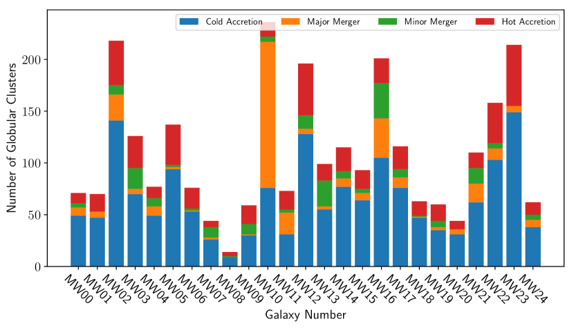
Figure 1: The formation environments of the $z=0$ GC populations in each of the 25 E-MOSAICS galaxies. The majority of GCs in every E-MOSAICS galaxy, except for MW10 and MW11, forms from gas which is smoothly accreted while cold, never exceeding $2\times 10^{5}\>{\rm K}$ prior to forming a GC. Both major and minor mergers only contribute a small fraction of the total number of GCs seen.

The E-MOSAICS simulations were introduced by Pfeffer et al. (2018); Kruijssen et al. (2019a), and described in detail in section 2 there. In brief, E-MOSAICS consists of 25 cosmological zoom-in simulations (Katz & White, 1993) of typical $L^{*}$, MW-like spiral galaxies. The simulations build on the successful EAGLE cosmological volume simulations (Schaye et al., 2015; Crain et al., 2015) by using the same set of physics for gas cooling and heating, formation of both stars and black holes, as well as feedback from the same. The details of the physics model used in both EAGLE and E-MOSAICS can be found in Crain et al. (2015) and Pfeffer et al. (2018), the enhanced hydrodynamics method anarchy is detailed in Schaye et al. (2015), and the results of the improvements are described in Schaller et al. (2015). The EAGLE simulations reproduce the galactic stellar mass function and size-mass relation (Baldry et al., 2012) through careful calibration of the star formation and feedback parameters used. This means that other galaxy properties and scaling relations, such as the cosmic star formation history, the black hole to stellar mass relation, mass-metallicity relation, and others are all predictions of the EAGLE physics model, rather than quantities that are explicitly tuned to match observations. The interplay of galaxy assembly and the star formation and feedback processes then emergently reproduce the star forming sequence (Crain et al., 2015), cosmic star formation history (Furlong et al., 2015), observed mass-discrepancy acceleration relation (Ludlow et al., 2017), HI-stellar mass relation (Crain et al., 2017), QSO absorption features (Oppenheimer et al., 2016; Turner et al., 2017), and mass-metallicity relation (De Rossi et al., 2017).

The EAGLE model uses the Wiersma et al. (2009) model for radiative cooling and heating, assuming ionisation equlibrium and a Haardt & Madau (2012) UV background. Star formation is handled using a a pressure-dependent reformulation of the Kennicutt (1998) star formation law (Schaye, 2004). The slope of the star formation relation $\dot{m}_{*}\propto P^{(n-1)/2}$ follows the standard Kennicutt slope of $n=1.4$ below $n_{H}<10^{3}\>{\rm cm^{-3}}$, but increases to $n=2$ at higher densities. Star formation is allowed to occur in gas which exceeds $n_{H}=0.1\>{\rm cm^{-3}}(Z/0.002)^{-0.64}$, where $Z$ is the local gas metallicity. A thorough discussion of this model, a justification of its parameters, and a comparison to simpler star formation models can be found in Schaye et al. (2015) and Crain et al. (2015).

The haloes simulated in E-MOSAICS are selected from the EAGLE Recal-L025N0752 volume, and re-simulated with a factor of 8 better mass resolution than the $100\>{\rm Mpc}$ EAGLE volume (corresponding to a factor of 2 better spatial resolution). The baryonic particle mass is $2.25\times 10^{5}\>{\rm M_{\odot}}$, with a Plummer-equivalent gravitational softening length of $1.33$ comoving kpc prior to $z=2.8$ and $350$ physical pc from that point forward. Merger trees are generated, as in Schaye et al. (2015) and Qu et al. (2017), using subfind (Springel et al., 2001) on the 29 snapshots saved between redshift 20 and 0.

The distinguishing feature that sets E-MOSAICS apart from EAGLE, or from the APOSTLE (Sawala et al., 2016) and Cluster-EAGLE (Barnes et al., 2017; Bahé et al., 2017) zoom-in simulations, which also use the EAGLE physics model, is the inclusion of a set of sub-grid physics models for the formation, evolution, and disruption of gravitationally bound stellar clusters (combined in the MOSAICS sub-grid cluster model Kruijssen et al. 2011; Pfeffer et al. 2018). These stellar cluster models are fully local, depending only on physical properties of the local environment, rather than disc or halo averaged properties, or non-local measurements (such as the identification of mergers). An in-depth discussion of these models for GC formation and evolution is presented in Pfeffer et al. (2018) and Kruijssen et al. (2019a), which we briefly summarise here. The cluster formation model in E-MOSAICS is determined by the theoretical model for the cluster formation efficiency (CFE) derived in Kruijssen (2012), which relates the CFE to the local gas volume density, velocity dispersion, and thermal sound speed, and reproduces the CFEs observed in nearby star-forming galaxies. Each star particle contains a population of clusters with an initial cluster mass function (ICMF) described by a Schechter (1976) function, with a ICMF truncation mass related to the maximum GMC mass (Reina-Campos & Kruijssen, 2017). This is set by the fraction of a locally-calculated Toomre mass which can collapse and form stars prior to being disrupted by feedback. Cluster evolution then consists of three major components: stellar evolution, using the same stellar evolution tracks as EAGLE, two-body relaxation, and tidal shocks. Two-body relaxation and tidal disruption rates are calculated using the locally-calculated tidal tensor (Gnedin, 2003; Prieto & Gnedin, 2008; Kruijssen et al., 2011), which allows on-the-fly calculation of cluster disruption based on the tidal environment they find themselves in. Finally, the dynamical friction timescale for a cluster to fall into the centre of the galaxy is calculated with a postprocessing algorithm (Pfeffer et al., 2018). If the dynamical friction timescale calculated is less than the age of the cluster, it is flagged as disrupted by dynamical friction.

The MOSAICS model for cluster formation and evolution has been used in a number of studies that have successfully reproduced many observed properties of GC populations. The cluster disruption used in MOSAICS has been shown to reproduce observed $z=0$ cluster distributions in age, space, and mass, as well as the kinematics of GC systems (Kruijssen et al., 2011, 2012; Adamo et al., 2015; Miholics et al., 2017). The simulated E-MOSAICS galaxies and GC populations reproduce the typical star formation history, specific frequency, metallicity distribution, mass function, spatial distribution (Pfeffer et al., 2018; Kruijssen et al., 2019a) and “blue tilt” (Usher et al., 2018) seen in local $L^{*}$ galaxies. The young stellar clusters in E-MOSAICS reproduce cluster formation efficiency and high mass truncation in the initial cluster mass function (Pfeffer et al., 2019b) observed in the local galaxy population.

The E-MOSAICS simulations have also been used to study a broad variety of questions in cluster and galaxy formation and evolution. They have been used to connect the galactic assembly history to the GC population in age-metallicity space (Hughes et al., 2019; Kruijssen et al., 2019a, b) and to the $\alpha$ element abundances of GCs (Hughes et al., 2020). E-MOSAICS has been used to predict the GC UV luminosity function (Pfeffer et al., 2019a), the overall formation history of clusters and GCs compared to field stars (Reina-Campos et al., 2019), and constrain the fraction of halo stars contributed by dynamical disruption of GCs (Reina-Campos et al., 2020).

3 The birth environment of globular clusters

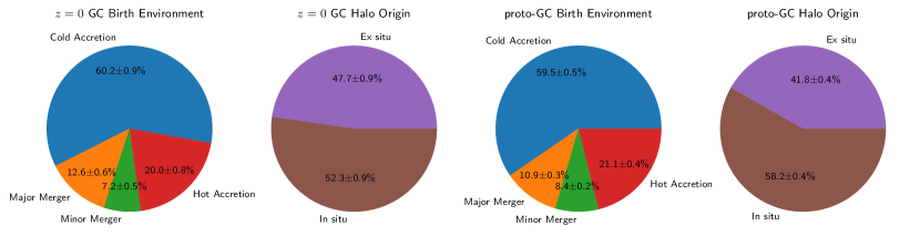
Figure 2: The birth environment and natal galaxy of both the present day GCs and all formed proto-GCs. For both the surviving GC population and the proto-GCs primarily form out of gas which has never been shocked above $2\times 10^{5}\>{\rm K}$, with $15-20$ per cent forming during major and minor mergers. Most proto-GCs and GCs at $z=0$ were formed in-situ ($58.2\pm 0.7$ per cent and $52\pm 1.0$ per cent, respectively). The larger fraction of in-situ proto-GCs indicates that proto-GCs formed in-situ experience stronger disruption over their lifetimes than those formed in satellites that were subsequently accreted.

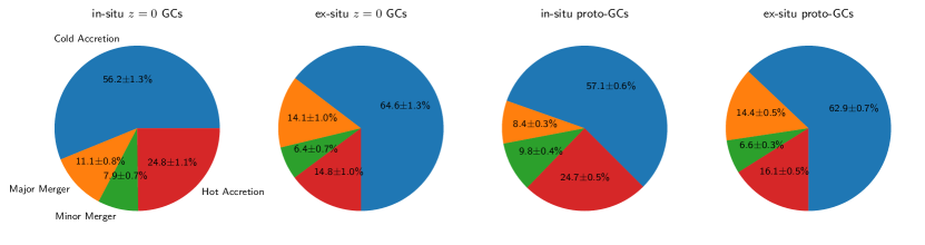
Figure 3: The birth environment for in-situ and ex-situ $z=0$ GCs and proto-GCs. In-situ clusters form within the “trunk” of the merger tree, while ex-situ clusters form in smaller haloes that are then accreted. The ex-situ population contains a roughly equal fraction of merger-formed GCs ($20.5\pm 1.2$ per cent as opposed to $19.1\pm 1.1$ per cent) and a lower fraction of GCs forming out of shock-heated gas ($15\pm 1$ per cent as opposed to $24.7\pm 1.1$ per cent). This is to be expected, as lower-mass haloes have lower virial temperatures.

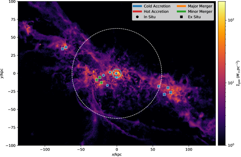
Figure 4: Gas column density in the environment of a typical GC-forming galaxy at $z=2.5$. Gas particles that will form GCs by the next snapshot are marked with coloured circles (in-situ) or squares (ex-situ), each indicating their formation channel (using the same colour scheme as in Figure 2 and 3). The virial radius of the galaxy is shown with the dashed white circle, and twice the stellar half-mass radius is shown with the solid cyan circle. The majority of the GCs that form at this time come from the cold, clumpy medium fed by the many visible filaments. A minor merger in the outskirts of the disc will produce 3 ex-situ GCs, and a single cluster is formed from gas which once exceeded a temperature of $2\times 10^{5}\>{\rm K}$. As can be seen, two smaller haloes will deliver 6 ex-situ clusters to the central galaxy when they later merge. These mergers will occur after these GCs form in the satellite galaxies.

We select $z=0$ GCs using the same criterion as Kruijssen et al. (2019a), namely that their masses must be $>10^{5}\>{\rm M_{\odot}}$, metallicities $\rm[Fe/H]$ between $-2.5$ and $-0.5$, and with galactocentric radii of $>3\>{\rm kpc}$, to select clusters that match observed GC properties and exclude clusters that likely have experienced underdisruption due to numerical effects (e.g. strongly softened gravity and importantly, under-resolved cold ISM clumps). With these selection criteria, we find 2732 GCs across the 25 E-MOSAICS galaxies. We also apply the same selection criteria, but rather than using the $z=0$ masses of the clusters, instead use their birth masses. This allows us to generate a population of “proto-GCs”, of clusters that would be identified as GCs at $z=0$ had they not experienced disruption due to their individual tidal histories (or lost mass due to stellar evolution). We find 12,186 of these proto-GCs, showing once again (as has been reported in Reina-Campos et al. 2018) that dynamical disruption plays as much of a role producing the present-day GC population as does the formation physics. For all quantities related to population fractions, we calculate a mean estimate and confidence interval using 1000 bootstrap samples (Efron, 1979).

3.1 Distribution of GCs across different formation channels

We split the populations of GCs and proto-GCs into a set of disjoint subsets (the union of which bijects the whole population). The first family is the birth environment, and contains four possible formation channels. A cluster can form during a merger event (either a major merger, with a stellar mass ratio above 1:4, or a minor merger with a stellar mass ratio between 1:4 and 1:10). We identify merger events by selecting subhaloes which formed through the merger of two or more subhaloes from the previous snapshot, and identify clusters which formed in that interval as forming during a merger. If a cluster does not form during a merger, it may form from gas that has never been strongly shock-heated above the $2\times 10^{5}\>{\rm K}$ peak of the cooling curve (gas that we identify as coming from “cold accretion”), or gas which has been heated above this temperature (gas we identify as brought to the galaxy by “hot accretion”). As this is near the peak of the cooling curve (due to efficient recombination cooling), gas will only be pushed above this temperature by feedback or a virial shock, and will usually persist well above or below this temperature (Brooks et al., 2009; Woods et al., 2014). This is also roughly the virial temperature that galaxies will reach once their halo mass exceeds $10^{11}\>{\rm M_{\odot}}$. As we simply track the maximum temperature a gas particle reaches prior to star formation, without a detailed analysis of the full thermal history, this temperature split will not perfectly map to gas accreted along cold flows vs. gas shock-heated at the virial radius. Heating from SNe can also generate temperatures above $2\times 10^{5}K$, and failure to capture brief shocks may miss brief excursions above $2\times 10^{5}\>{\rm K}$. Rather than specifically referring to gas accreted along cold streams as opposed to gas heated by a virial shock, our “cold accretion” and “hot accretion” populations are more accurately described simply as gas which was always cold as opposed to gas that was previously heated. Naturally, since star formation in the EAGLE model occurs when gas cools below the $8000\>{\rm K}$ equation-of-state threshold, gas that will form “hot accretion” GCs must cool before star formation actually occurs. We also split the population of GCs and proto-GCs based on whether they form in the largest progenitor of the $z=0$ galaxy (“in-situ” clusters, in the trunk of the merger tree), or in one of the smaller progenitors (“ex-situ” clusters, formed in the branches of the merger tree).

In Figure 1, we show the number of clusters formed through each of these four channels for the 25 E-MOSAICS MW analogues. The majority of GCs in each galaxy (except for MW10) form outside of merger events, with most of these forming from gas which has never been heated above $2\times 10^{5}\>{\rm K}$. It is also clear here that for MW-mass galaxies, there is fairly significant scatter of both the fraction of GCs formed through each channel, and the total number of GCs formed (this has been previously shown explicitly in figure 2 of Kruijssen et al. (2019a), and is implied by studies of the specific frequency of GCs, such as Peng et al. 2008). As Figure 2 shows, both the $z=0$ GC population, as well as the proto-GCs form primarily outside of merger events ($>80$ per cent of each population), and mostly from gas accreted onto their parent galaxy without being heated. Galaxy mergers appear to be a fairly minor contributor to the GC population, accounting for $15-20$ per cent of the proto-clusters that are formed, as well as the fraction of those which survive to $z=0$.

In Figure 2, we also show the fractions of GCs and proto-GCs that form in-situ or ex-situ. The fraction of proto-GCs formed in-situ is somewhat larger than the fraction of in-situ GCs that survive to $z=0$ ($58.2\pm 0.7$ per cent vs. $52.3\pm 1.3$ per cent). This tells us that the disruption mechanisms that destroy $\sim 80$ per cent of the proto-GCs before $z=0$ are more effective for in-situ clusters than ex-situ clusters. A deeper potential well, as well as higher ISM densities in the larger primary progenitor may help explain these differences, because of the increased rate of cluster disruption and tidal shocks.

We can also separate the in-situ and ex-situ populations based on the four formation channels previously examined. In Figure 3, we show the fraction of each formation channel producing the in-situ and ex-situ GCs and proto-GCs. Once again, there is little difference between the breakdown of formation channels between the surviving $z=0$ GCs and the proto-GCs. We do, however, see a noticeable difference between the in-situ and ex-situ populations. Ex-situ clusters are more formed in major mergers ($14.1\pm 0.9$ per cent in ex-situ, as opposed to $11.1\pm 0.9$ per cent for in-situ), and less often from gas that has been shock-heated ($14.8\pm 1.0$ per cent for ex-situ as opposed to $24.7\pm 1.1$ per cent for in-situ). We verify that this is not simply an effect of the different median formation times by looking at only clusters formed before $z=1$, and find similar fractions. The lower fraction formed by shock-heated gas is easily understood: the less-massive haloes in which these clusters form had virial temperatures below $2\times 10^{5}\>{\rm K}$, and the stellar feedback that could alternatively heated gas was less intense in the less active star formation environment of these lower-mass haloes. The larger fraction being formed by mergers is interesting, as it suggests that these smaller, accreted galaxies were less likely to produce the high ISM pressure and density required to form GCs outside of merger events.

An example of the qualitative morphology of a typical galaxy in which the majority of GCs form is shown in Figure 4, which shows the gas surface density in the progenitor halo of MW00 at $z\sim 2.5$. The bulk of the clusters formed between this snapshot and the next are formed in-situ, from cold accreted gas. A handful of ex-situ clusters will also be delivered to the central galaxy, from the two satellites falling in along the two primary filaments. These clusters will form in the two satellites prior to their merging with the central halo, and form from gas that has never been shock heated. Dense gas in this galaxy clearly extends well past the stellar half-mass radius, and is in a turbulent, highly disrupted state. The single example of a cluster formed from shock-heated gas is a case where the heating comes not from a virial shock, but from stellar feedback, as the virial temperatures of all haloes in this snapshot are $<2\times 10^{5}\>{\rm K}$.

3.2 Properties of globular clusters formed through different channels

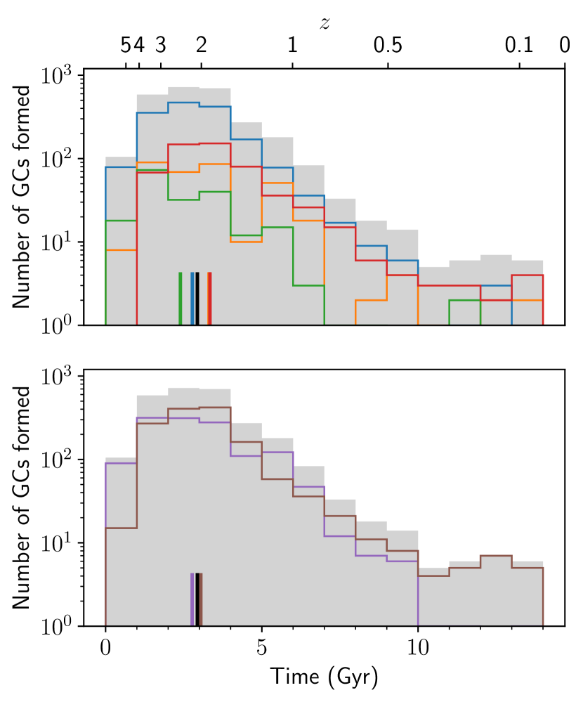
Figure 5: Formation times for $z=0$ GCs as a function of their formation channel (top) and whether the clusters formed in-situ vs. ex-situ (bottom). The top histogram shows the formation times for all GCs (grey), those formed in major mergers (orange), those formed in minor mergers (green), those formed by gas that was never shock-heated above $2\times 10^{5}\>{\rm K}$ (blue), and those formed by gas that was shock-heated (red). The vertical lines show the median formation times for each channel. The typical GC forms at $z=2$, roughly $11.3\>{\rm Gyr}$ ago. The bottom histogram shows the same quantities, but split based on whether the cluster forms in-situ (brown) or ex-situ (purple). Here it can be seen that the formation rates as a function of time for both in-situ and ex-situ clusters are relatively similar.

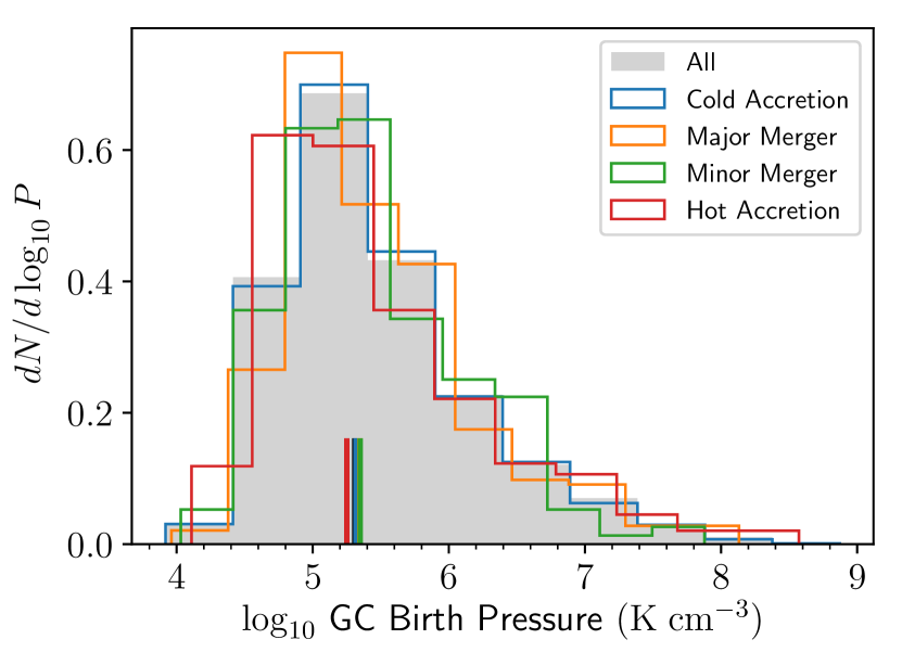
Figure 6: Distribution of ISM birth pressure for GCs as a function of their formation channel. The distribution of birth pressures for all GCs (grey), those formed in major mergers (orange), those formed in minor mergers (green), those formed by gas that was never shock-heated (blue), and those formed by gas that was shock-heated (red) are effectively indistinguishable. Regardless of what the state of the galaxy is, or how the gas which forms the GC is accreted onto the galaxy, the distribution of birth pressures is effectively the same, with the average GC forming from gas with $P/k_{\rm B}=10^{5.3\pm 0.9}\>{\rm K}\>{\rm cm^{-3}}$.

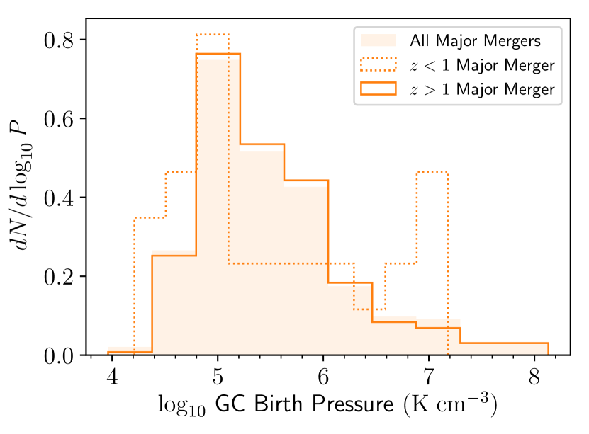
Figure 7: Distribution of ISM birth pressure for GCs formed in major mergers. The solid histogram shows all GCs formed in major mergers, the dashed line shows GCs formed in major mergers after $z=1$, and the solid line shows GCs formed in major mergers before $z=1$. The old GCs make up the majority of the population that formed in major mergers, and thus track the average pressure distribution. Notably, the young major merger-born GCs show a distinct bimodal distribution, with a high-pressure population forming from gas with pressures of $P/k_{\rm B}\sim 10^{7}\>{\rm K}\>{\rm cm^{-3}}$.

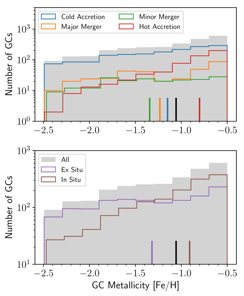
Figure 8: Metallicity distributions of GCs as a function of formation channel (top) and in-situ or ex-situ formation (bottom). As the top panel shows, GCs formed through mergers have a much flatter metallicity distribution than those formed through smooth accretion (whether that accretion is cold or hot). Clusters formed through hot accretion have the steepest metallicity distribution, with the vast majority having high metallicities. GCs formed during major mergers show a nearly uniform metallicity distribution. In the bottom panel, we see that the clusters formed ex-situ have significantly lower metallicities than those formed in-situ, as well as having a much flatter metallicity distribution. Clusters with metallicity $\rm[Fe/H]<-1.5$ are dominated by the ex-situ component.

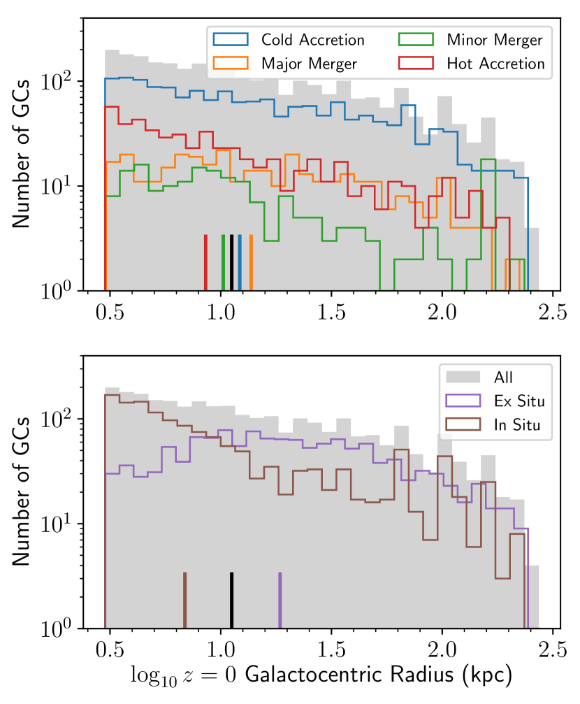
Figure 9: Galactocentric radii of GCs as a function of formation channel (top panel) and in-situ vs. ex-situ formation (bottom). As the top panel shows, GCs formed through smooth accretion (red and blue curves) have a more centrally peaked radial distribution, with the median cluster falling at galactocentric radii of $\sim 10\>{\rm kpc}$, while those formed through mergers (orange and green curves) fall into a nearly uniform radial distribution. In the bottom panel, we see this is even more pronounced when we differentiate between in-situ and ex-situ clusters.

The natural question these channels raise is whether populations of GCs formed in each channel share properties that are distinguishable from populations formed through the other channels, and whether these differences are potentially observable. Looking simply at when the present-day clusters are formed through each channel, as we do in Figure 5, we see that most GCs are formed between $z=1.5-5$, when the Universe was less than one third of its current age (also see Reina-Campos et al. 2019). We can also see noticeable transitions between the frequency of GCs formed through each of the four channels we examine. While the majority of GCs form from unshocked gas outside of merger events at nearly every epoch, the youngest population of clusters (especially those formed after $z=1$) is increasingly composed of those formed during major mergers and from shock-heated gas (prior to $z=1$, $>60$ per cent of clusters form from cold accretion, versus $\sim 50$ per cent after $z=1$). The oldest population is those formed in minor mergers, with a median birth time of $2.39\>{\rm Gyr}$ after the Big Bang, while the youngest is those formed through major mergers, with a median formation time of $3.34\>{\rm Gyr}$. GCs formed from previously heated gas have a median formation time of $3.31\>{\rm Gyr}$, and those formed from unheated gas have a median formation time of $2.77\>{\rm Gyr}$. The median formation time for all GCs is $2.93\>{\rm Gyr}$. We would expect the increase in shock-heating as the haloes become more massive and their virial temperatures increase, as well as more opportunities for feedback heating as the ISM is recycled in galactic fountains. Interestingly, the component formed from minor mergers is almost entirely formed prior to $z=1$, making them (on average) the oldest population, along with those which are formed from cold-accreted gas. For in-situ vs. ex-situ clusters, however, we see no difference in the median formation times, with both populations roughly tracking the total formation rate, and with median formation times comparable to each other.

If we look at the ISM property which primarily sets the cluster formation efficiency ($\Gamma$), the pressure, we see in Figure 6 little difference between clusters formed through each of our channels. The ISM birth pressures for GCs formed from each of the examined channels (as well as the full population) have nearly identical distributions. The median ISM pressure which $z=0$ GCs are formed is $P/k_{\rm B}=10^{5.3\pm 0.9}\>{\rm K}\>{\rm cm^{-3}}$. This distribution has noticeable skewness, with a long tail of clusters formed form pressures as high as $P/k_{\rm B}=10^{9}\>{\rm K}\>{\rm cm^{-3}}$. We can also see the enhanced pressures that are observed with YMC formation sites at low redshift in Figure 7. At low redshift, major mergers can form a larger fraction of GCs from much higher pressures than at earlier times, producing a distinct population of GCs formed at pressures of $P/k_{\rm B}\sim 10^{7}\>{\rm K}\>{\rm cm^{-3}}$. The higher collision velocities and more massive galaxies involved in recent major mergers make these events more violent, compressing the ISM to higher pressures (but for shorter time periods) than what is typical at higher redshifts.

If we look in Figure 8 at the metallicity of the clusters, probed through their iron abundances, we see a few notable features of our different formation channels. For all metallicity bins, GCs formed through cold accretion make the largest fraction of GCs. The metallicity distribution for clusters formed through minor mergers is nearly flat, resulting in the lowest median metallicity of $\rm[Fe/H]\sim-1.3$, while the metallicity distribution for clusters formed after being shock-heated is strongly biased towards metal-rich GCs, with a median $\rm[Fe/H]\sim-0.80$. These medians are somewhat unsurprising when we consider that minor mergers are frequent at high redshift (when the cosmic metallicity was lower), and will tend to bring relatively pristine gas in with the smaller merging partner (as the smaller partner, following the mass-metallicity relation, will have lower overall metallicity, see e.g. Erb et al. 2006). For GCs formed from previously shock-heated gas, this gas was either heated through a virial shock, implying the halo mass $>10^{11}\>{\rm M_{\odot}}$, and thus a much more metal-enriched ISM (assuming that the mass-metallicity relation holds), or through SN feedback, which brings with it fresh metals in the form of the SN ejecta. As GCs of all metallicities are primarily formed outside of mergers, from unshocked gas, we cannot easily use a simple metallicity criterion to determine observationally whether a cluster is formed through a given channel.

We do, however, see that if we look at metallicity for in-situ or ex-situ clusters, the median metallicity for in-situ clusters is larger ($\rm[Fe/H]\sim-0.9$ as opposed to $\rm[Fe/H]\sim-1.3$), and the distribution is much steeper. While some individual E-MOSAICS galaxies show bimodal MW-like GC metallicity distributions, we see here that neither the full population across all 25 galaxies, nor the population of in-situ or ex-situ GCs is simply bimodal. We do see that extremely metal poor GCs, with $\rm[Fe/H]<-1.5$ are dominated by ex-situ GCs. Despite this, if we look at metal rich vs. metal poor GCs, we cannot simply split the population based on their origin as in-situ or ex-situ. Both scenarios contribute significant numbers of GCs, and as Kruijssen et al. (2019a) showed, the old and metal-poor GC populations show a roughly equal contribution of in-situ and ex-situ GCs. Generally, ex-situ GCs tend to be lest metal rich than in-situ GCs as a consequence of the mass-metallicity relation and the fact that, for a given formation time, in-situ GCs form in more massive haloes than ex-situ ones (by definition). The fact that in-situ clusters have typically formed in more massive objects (as indicated by their higher metallicity) helps to explain their more effective disruption: more massive objects will have stronger tides, and a greater chance for close encounters with the ISM of the disc. When the GCs are young, and subject to the most intense tidal shocks from their natal environment (the dense ISM), this deeper potential will make it more difficult for them to be ejected from the disc.

Turning to the spatial distribution of GCs , we see in Figure 9 that there is a noticeable difference between GCs formed through different channels, but again at all radii the population is dominated by clusters formed through cold accretion. The most centrally concentrated population are those formed through hot accretion, as we might expect from their higher metallicity and the metallicity gradient observed in both real GC systems and the E-MOSAICS galaxies. Clusters formed through mergers have a broader distribution, with GCs formed in a major merger lying at a median radius of $\sim 12\>{\rm kpc}$. In-situ clusters have a median galactocentric radius of $\sim 7\>{\rm kpc}$, while ex-situ clusters have median radii of $\sim 18\>{\rm kpc}$. Interestingly, we can also see that a slim majority of GCs in the outer halo, beyond $10\>{\rm kpc}$, are accreted ex-situ clusters. We also see that in-situ clusters can be deposited up to $\sim 100\>{\rm kpc}$ from the galaxy.

3.3 The galaxies that form GCs

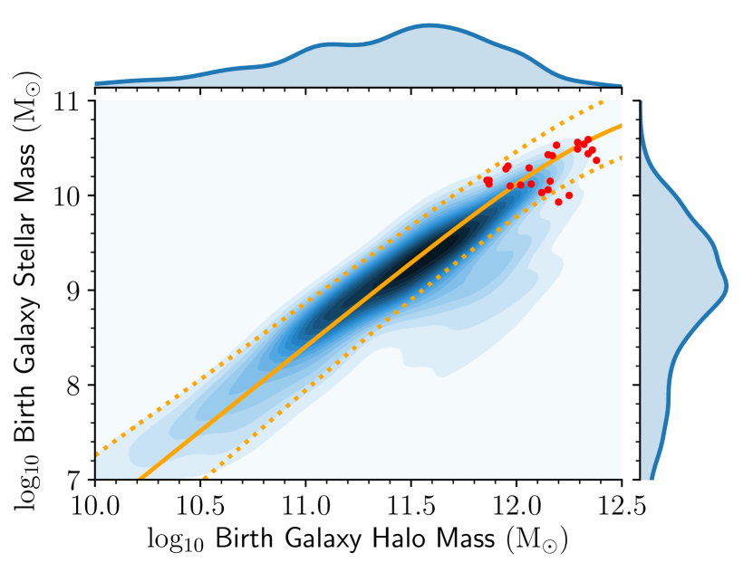
Figure 10: The relation between stellar mass and halo mass for haloes in which GCs are formed. The main panel shows contours of the number of GCs formed, with Kernel Density Estimates (KDEs) shown for the halo and stellar mass above and to the right. The median GC forms in a halo with virial mass $M_{200}=10^{11.5\pm 0.7}$ and stellar mass $M_{*}=10^{9.0\pm 1.1}$. The orange lines show the Moster et al. (2013) SMHMR at $z=2$ (median in solid, scatter in dotted). Red points show the final halo and stellar masses of the E-MOSAICS galaxies at $z=0$. The vast majority of GCs form in relatively massive haloes (rather than low mass dwarfs), which lie on the typical SMHMR for the median GC formation redshift, $z\sim 2$. The scatter seen in the E-MOSAICS haloes is in part due to them forming at a variety of redshifts, while the overplotted curves are for haloes at a single redshift ($z=2$), but also due to the intrinsic scatter in the SMHMR.

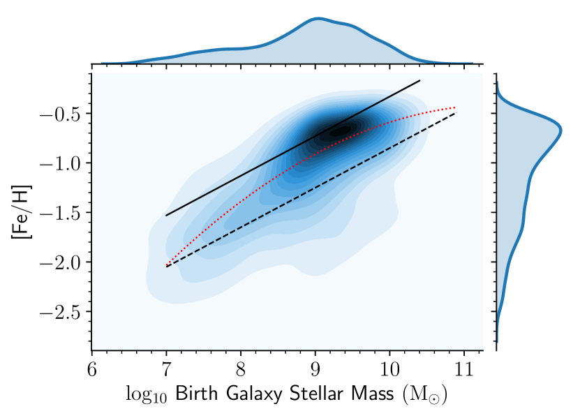
Figure 11: Globular cluster metallicity versus stellar mass of its birth galaxy. There is a close relation between the metallicity of $z=0$ GCs and the stellar (and therefore halo) mass of the galaxy they form in, an indication that GCs can “lock in” the galaxy mass-metallicity relation, indicating directly the mass of the galaxy they formed in through their present metallicity. The solid and dashed curves show the z$=0$ and $z=3$ galaxy mass-metallicity relations from the Ma et al. (2016) simulations, while the red dotted curve shows the mass-metallicity relation at $z=2$ derived in Kruijssen (2014) from observations by Erb et al. (2006) and Mannucci et al. (2009).

As we have seen, most globular clusters are formed in-situ, in between periods of major or minor mergers. Figure 10 shows us that the galaxies GCs are born within fall well on the abundance-matched host stellar mass–halo mass relation (SMHMR) of Moster et al. (2013) for the typical redshift at which most of our GCs form ($z\sim 2$). There is a relatively broad distribution in both the stellar and halo masses of the galaxies in which GCs form, with typical virial masses of $M_{200}=10^{11.5\pm 0.7}\>{\rm M_{\odot}}$ and stellar mass $M_{*}=10^{9.0\pm 1.1}\>{\rm M_{\odot}}$.

We have already seen that there are some noticeable differences in the metallicity distribution of GCs formed through different channels, and whether those clusters form in-situ or ex-situ. In Figure 11, we show that the metallicity of $z=0$ GCs trace, with significant scatter, the stellar mass of their birth galaxy (also see Kruijssen et al., 2019a, b). The metallicity of GCs is slightly above the average ISM metallicity we would expect from the mass-metallicity relation at $z\sim 2$, when most GCs form. This is indicative of correlated star formation producing GCs: i.e. they form within regions where previous star formation activity has enriched their natal gas with metals. The birth galaxy mass-GC metallicity relation explains most of the differences between GCs of different origins seen in Figure 8. Clusters which are formed in accreted satellites, or at higher redshift in minor mergers, will have lower metallicity if their birth galaxy follows the mass metallicity relation (as those birth galaxies will be less massive).

The local ISM that forms GCs naturally must be able to produce the pressures we see in Figure 6. In Figure 12 we look at the cold gas fraction $f_{\rm gas}=M_{\rm cold}/(M_{\rm cold}+M_{*})$ in the subhaloes where GCs form. Cold gas in this case is identified as gas below the temperature threshold for star formation in E-MOSAICS, $2.5\times 10^{4}\>{\rm K}$. The majority of GCs form in extremely gas-rich discs ($f_{\rm gas}=0.6\pm 0.2$). We see also a decreasing trend in gas fraction as we move to lower redshift, as shown by observations of high-redshift, star-forming galaxies (Tacconi et al., 2013). These gas fractions may be larger than those observationally determined, as we are measuring the total cold gas content of the subhalo, rather than the observationally-detected cold gas (traced by HI and CO, where the latter dominates at these gas pressures) within the stellar disc. This means we will include cold gas within the circumgalactic medium that might otherwise be missed by looking only within the disc of the galaxy, though this is likely a small minority.

For in-situ GCs, we can now look at how the assembly history of the galaxy redistributes them onto new orbits. In Figure 13, we can see how this radial shuffling takes place, comparing the galactocentric radius at formation to the galactocentric radius at $z=0$. Naturally, if GCs have highly eccentric orbits, we will find them at different galactocentric radii at different times. GCs on eccentric orbits spend more time at large radii, so we would expect to find most GCs at larger radii than their formation radius. On the other hand, GCs forming in growing haloes will find their orbital radii decreasing over time as the depth of the potential well increases. Figure 13 shows that this effect (the compaction of the GC system as the halo grows) is detectable in the change in GC radii, with more GCs migrating onto smaller (rather than larger or identical) radii between when they form and when we could observe them at $z=0$. As the ex-situ clusters are deposited on relatively larger radii than where they formed, the relative reduction of in-situ clusters at $r>10\>{\rm kpc}$ is compensated through the ex-situ clusters, which are distributed nearly uniformly through the halo (as is shown in Figure 9).

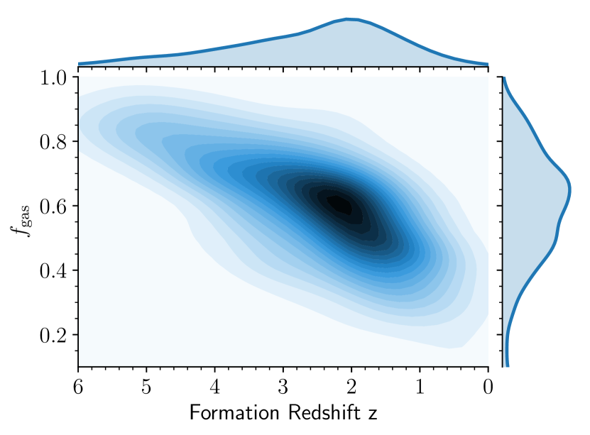
Figure 12: Subhalo gas fraction as a function of formation redshift of GCs. The majority of GCs form in highly gas-rich discs $f_{gas}>0.5$, regardless of redshift. However, a small fraction of GCs forms out of more stellar-dominated discs, predominantly at later redshifts, once sufficient time has passed to build up a stellar disc.

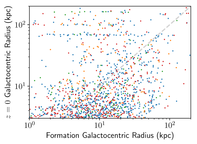
Figure 13: Final position at $z=0$ as a function of formation position for all in-situ GCs in E-MOSAICS, coloured by formation mechanism. The light grey line shows the 1-to-1 line we would expect if GCs remained on the same orbital radii as they formed. There is a tremendous amount of re-shuffling for all of the different formation mechanisms, with no obvious difference between them. It is also clear that the majority of clusters end up on closer orbits at $z=0$ than they are born on. This is somewhat to be expected from the evolution of the galaxy, as a GC with constant orbital energy will find itself in a tighter orbit as the halo mass grows. The horizontal lines seen near $\sim 100\>{\rm kpc}$ are dwarf satellites that are within the primary halo’s virial radius.

3.4 Birth environment and cluster survival

The trends we have seen in the $z=0$ GC population are a function of both the relative efficiencies of different GC formation mechanisms and the ability of proto-GCs to survive to the present time. We have already seen in Figure 2 that accreted proto-GCs are more likely to survive than in-situ proto-GCs. Proto-GCs formed in minor mergers are somewhat less likely to survive than the average proto-GC (they make up $8.4\pm 0.3$ per cent of formed proto-GCs, but only $7.2\pm 0.5$ per cent of the $z=0$ GCs), while those formed in major mergers are more likely to survive ($10.9\pm 0.3$ per cent of proto-GCs form in major mergers, compared to the surviving fraction of $12.5\pm 0.7$ per cent of $z=0$ GCs).

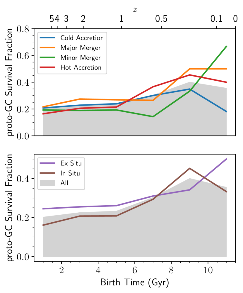
Figure 14: Fraction of proto-GCs that survive to $z=0$ as a function of time. For all GC formation mechanisms, we see an increase in the survival fraction over time owing to the fact that younger clusters form in a less disruptive environment (and have simply had less time to experience mass loss). As is clear from the top panel (survival fraction split based on formation mechanism), all formation channels see roughly similar survival rates, with major mergers having the highest survival rates during the peak of GC formation, $z>1$, and with minor mergers having the lowest survival rate. For the same time period, we also see in the bottom panel a higher survival rate for ex-situ, accreted proto-GCs.

In Figure 14, we examine the survival rate of proto-GCs formed in different channels over time. As we might expect, the average survival rate increases over time, as younger clusters have simply had less time to be disrupted than older clusters, and galaxies become less disruptive as they age and their ISM pressure drops. For the epoch when proto-GC formation is the most efficient, $z>1$, we can see that the differences in GC disruption seen in Figure 2 are reflected here. The survival rate of in-situ clusters is lower than of ex-situ clusters, those born in major mergers have the highest survival rate, and those born in minor mergers have the lowest survival rate. A proto-GC formed during the period of efficient GC formation had a relatively small chance of surviving to $z=0$, of about $20$ per cent. This is reflected in the overall survival fraction of $\sim 22$ per cent.

The survival fractions as a function of metallicity, shown in Figure 15, also shows the overall higher survival rate for ex-situ clusters. We see here as well that metal-rich clusters have lower survival fractions than metal-poor clusters for all of the populations we examine, except for a slight bump in the metal-rich clusters formed in major mergers. Some of these clusters correspond to the relatively late-forming population seen in Figure 5, and their high survival fraction is likely an artefact of their young ages. When we consider the decreasing survival rate as a function of metallicity along with the mass-metallicity relation shown in Figure 11, what we are seeing here is that more massive haloes (in which more metal-rich clusters form) subject their proto-GCs to stronger disruption than less massive haloes.

Figure 16 shows a significant trend in survival fraction as a function of the final galactocentric radii at which proto-GCs find themselves. We use the position of star particles that host disrupted clusters at $z=0$ to assign the radii of proto-GCs at $z=0$. Here we can see that we again have a universal trend in proto-GC survival, regardless of formation mechanism. Proto-GCs that are found in the stellar halo at $z=0$ have significantly higher survival rates (roughly a factor of 5 larger) than those found near the galactic disc. As proto-GCs are disrupted through tidal interactions (both smooth tides and tidal shocks), the closer they are to the denser environment of the galactic disc, the stronger their tidal mass loss will be. Those GCs we see in the halo at $z=0$ have likely spent a significant amount of time at large galactocentric radii, and thus have spent much of their lifetimes in a much gentler tidal environment than those we see closer to the disc. The most significant period of tidal disruption occurs early in the proto-GCs lifetime, when it is still embedded in the dense ISM. GCs that spend longer in the disruptive environment of the ISM prior to ejection will find themselves, on average, at smaller galactocentric radii (as the potential well will have grown deeper).

The disruption of clusters has been predicted (Gieles et al., 2006; Elmegreen & Hunter, 2010; Elmegreen, 2010; Kruijssen et al., 2011; Kruijssen, 2015) to be dominated by tidal shocks in the natal environment, as clusters move through the dense, high-pressure ISM in which they form. The strength of these tidal shocks increases at higher ISM densities and pressures. As Figure 17 shows, we see exactly this effect in the survival fraction of proto-GCs as a function of birth pressure. At higher pressures, significantly fewer proto-GCs are able to survive to $z=0$, with essentially all clusters formed at $P/k_{\rm B}>10^{9}\>{\rm K}\>{\rm cm^{-3}}$ being destroyed by tidal shocks. Interestingly, the only sub-population of GCs that show high survival fractions when formed from high pressures are those formed during major mergers. This has been predicted as a natural outcome of cluster migration (Kruijssen et al., 2011, 2012). Major mergers can “save” proto-GCs from disruption by depositing them into tidal tails, transporting them out of the dense ISM into the halo on a timescale shorter than the timescale required for disruption by tidal shocks, i.e. $\sim 100\>{\rm Myr}$. This is why we see a larger overall survival rate for clusters formed in major mergers, especially those formed at higher ISM pressure.

These trends all help explain the different survival rates we see for each of the different formation mechanisms in Figure 2. Ex-situ clusters have greater survival fractions than in-situ clusters, because they form in lower-mass haloes (as we would expect from Figure 8 based on their lower metallicity and the mass-metallicity relation from Erb et al. 2006) and orbit on much larger galactocentric radii (as we see in Figure 9). Despite forming in lower-mass haloes, proto-GCs formed through minor mergers are relatively old, and the merger events that form them were less likely to fling them out to large galactocentric radii than those proto-GCs formed in major mergers. This, combined with the population of relatively young GCs formed in late major mergers gives us the somewhat surprising result that proto-GCs formed during minor mergers are less likely to survive to $z=0$ than those formed in major mergers. The simple trends we see in age or metallicity for different formation mechanisms are not enough, a priori, to predict the survival rates of different mechanisms. The effect of disruption on proto-GC survival has a non-trivial effect on the distribution of clusters we see at $z=0$. The decreasing survival rate as a function of metallicity has the effect of flattening the metallicity distribution, as the survival rate as a function of metallicity has the opposite slope to the initial metallicity distribution. The same is true for the survival rate as a function of radius, with the increasing survival at high radii acting to flatten the radial profile by increasing the disruption rate of the disc clusters.

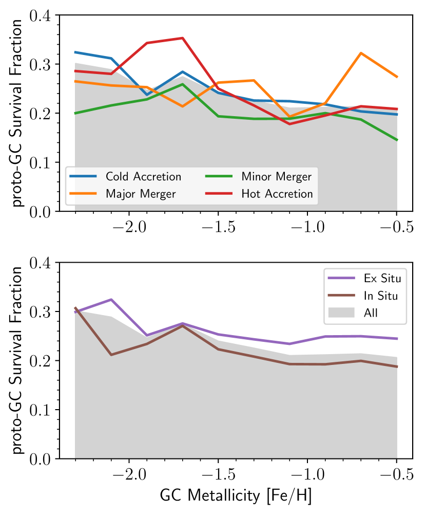
Figure 15: Survival fraction of proto-GCs as a function of their metallicity. As with the previous figures, the top panel shows the survival fractions split based on formation mechanism, while the bottom panel shows survival fractions split based on halo origin (in-situ or ex-situ). For all proto-GCs, regardless of their formation mechanism, we see a decrease in the survival fraction towards higher metallicities. Again, we see that proto-GCs formed in minor mergers have the lowest survival rates, and those formed ex-situ have higher survival rates than those formed in-situ.

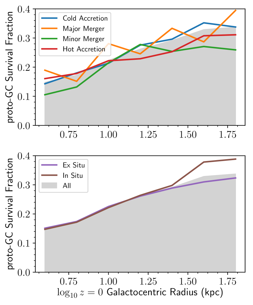
Figure 16: Survival fractions of proto-GCs as a function of their $z=0$ galactocentric radius. Proto-GCs that form closer to the centre of their parent halo experience stronger tidal interactions, producing a significantly rising survival fraction as a function of radius. Proto-GCs that are found at the edge of the halo are $\sim 5$ times more likely to survive to $z=0$ than those which are found near the galaxy disc. We see little difference in this relation between in-situ and ex-situ clusters, while the trend of lower survival rates for proto-GCs formed in minor mergers is again evident. Even for distant halo GCs, the survival fraction is $<40$ per cent, a result of the early disruption in the disc, prior to their ejection to large galactocentric radii.

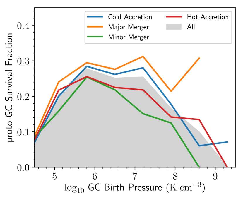
Figure 17: Survival fractions of proto-GCs as a function of birth pressure. The decreasing survival fraction, from $\sim 30$ per cent at $P/k_{\rm B}\sim 10^{6}\>{\rm K}\>{\rm cm^{-3}}$ to $\sim 5$ per cent at $P/k_{\rm B}\sim 10^{8}\>{\rm K}\>{\rm cm^{-3}}$ is evidence of the “cruel cradle” effect. This process is stronger at higher ISM density and pressure, and as a result proto-GCs formed from high pressures are less likely to survive to $z=0$, as they are destroyed rapidly by tidal shocks from dense clouds in the ISM. A major reason for the “bump” at high pressures seen in the proto-GCs formed through major mergers is the formation of more GCs from high-pressure gas in low redshift major mergers vs. high-redshift major mergers. As figure 14 shows, younger proto-GCs have larger survival fractions, meaning these proto-GCs have a higher survival rate simply due to their young age.

4 Do globular clusters form in substructure or minihalo collisions?

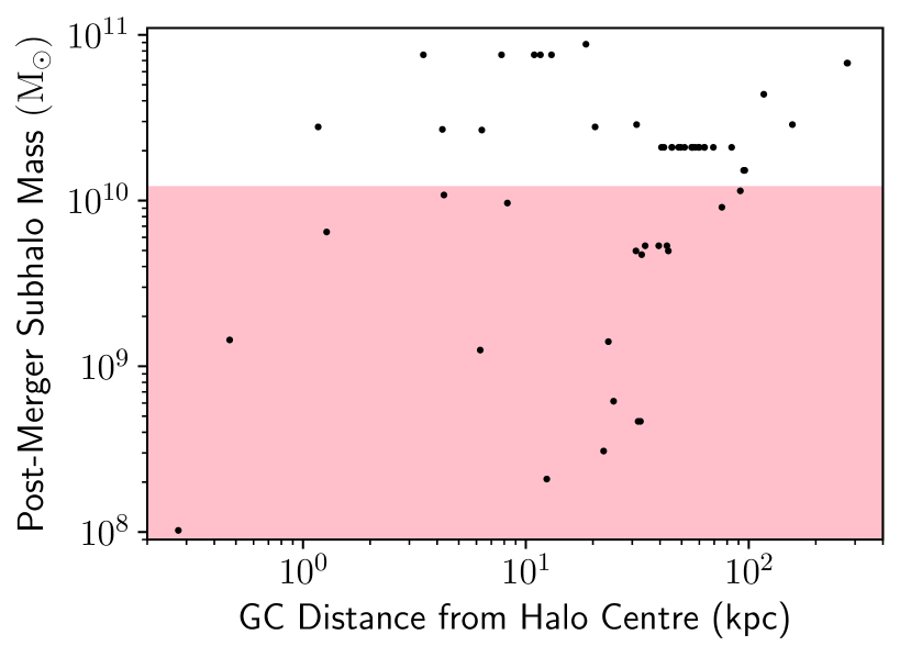
Figure 18: The mass of subhaloes produced by collisions of other subhaloes and form GCs as a function of the GC’s distance from the centre of potential of the primary halo the subhalo resides in. Most collisions occur between $10\>{\rm kpc}$ and $100\>{\rm kpc}$, and the median mass of the post-collision subhalo is $2.2\times 10^{10}\>{\rm M_{\odot}}$. Haloes affected by resolution (i.e. those with fewer than $10^{4}$ dark matter particles) are shown in the transparent red region. A significant fraction of these identified collisions are poorly resolved, and may be subject to significant numerical error.

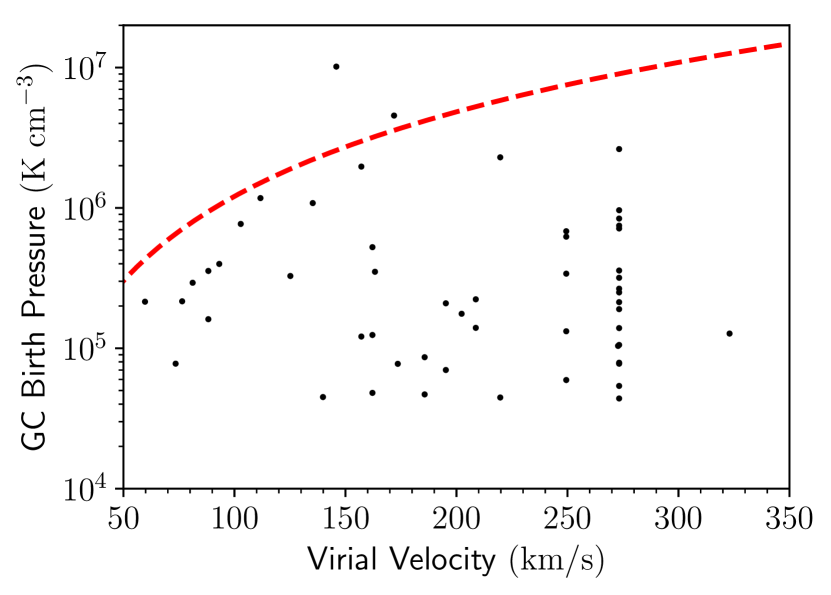
Figure 19: Birth pressure of GCs formed by subhalo collisions as a function of the virial velocity of the primary halo that contain those subhaloes. Black points show the true GC birth pressures, while the red dashed line shows the ram pressure produced by head-on collisions of subhaloes with ISM density of $1\>{\rm cm^{-3}}$ at the virial velocity of their parent halo. Only two clusters are formed at higher pressure than can be produced by the collision, whereas the majority of clusters can easily form through collisions at lower speed or with lower averaged ISM pressure.

One proposed mechanism (Smith, 1999; Madau et al., 2019) for the formation of GCs is through the collisions between subhaloes which then causes their gas to decouple from their dark matter (a small-scale analogue of the archetypical Bullet Cluster scenario, see Clowe et al. 2004). These clusters would actually form far from the disc, without the need for mergers and tidal encounters to deposit them into the halo and that way ensure their long-term survival.

The recent theoretical work of Madau et al. (2019) has sought to explain the specific observational facts we now have for the GC systems in the MW and M31. Namely, that observations of GCs in the outskirts of the galaxy halo, such as MGC1 have put strong constraints on the amount of dark matter these clusters may contain, consistent with them lacking any dark halo at all (Conroy et al., 2011). Madau et al. (2019) propose that a simple model for producing these dark matter free halo GCs that relies on two basic assumptions: that GCs form when gas pressures reach $P/k_{\rm B}\sim 10^{6}-10^{7}\>{\rm K}\>{\rm cm^{-3}}$, and that these pressures can be achieved through the collision of cool atomic clouds with densities of $\sim\>{\rm cm^{-3}}$ in substructure of the haloes of $L^{*}$ galaxies, where orbital velocities of $\sim 200\>{\rm km}\,{\rm s}^{-1}$ are sufficient to produce these conditions through ram pressure. The high pressures assumed for this model are justified by the fact that above $10^{7}\>{\rm K}\>{\rm cm^{-3}}$, the CFE approaches unity. The authors estimate, based on analytic kinetic theory and N-body simulations, that a few hundred of these collisions will occur within the halo of $L^{*}$ galaxies, most of which will have relative velocities sufficient to produce the high pressures they require. Of course, the alternative hypothesis for explaining the above observations is the one we obtain from E-MOSAICS, namely that GCs form as the natural outcome of high-redshift star formation in a way that is fundamentally unassociated with dark matter.

A similar proposed mechanism, albeit at higher redshift, is the collision of atomic cooling minihaloes (with virial masses $\sim 10^{8}\>{\rm M_{\odot}}$) at high redshift, prior to the formation of stars within said haloes (Trenti et al., 2015). In this mechanism, GCs form as the nuclei of these minihaloes after a major merger, with a dark matter halo surrounding them, and with re-enrichment of a second generation of stars fed via slow stellar winds. The dark matter halo is subsequently stripped away by the assembly of the main halo they fall into. While this chemical enrichment scenario is not one we can probe with the single phase of cluster formation intrinsic to the MOSAICS model, we can quantify the frequency of GC formation in minihalo collisions.

Since the mechanisms proposed by Trenti et al. (2015) and Madau et al. (2019) rely only on simple hierarchical structure formation and hydrodynamics, it should in principle manifest itself in the E-MOSAICS simulations, with some important caveats. Firstly, the E-MOSAICS simulations are run at a significantly lower dark matter resolution than the Via Lactea I simulations studied in Madau et al. (2019) ($1.6\times 10^{6}\>{\rm M_{\odot}}$ as opposed to $2.1\times 10^{4}\>{\rm M_{\odot}}$ respectively) or the simulations used in Trenti et al. (2015) (which used a mass resolution of $8.3\times 10^{4}\>{\rm M_{\odot}}$). This means that many of the subhaloes we identify, as well as the majority of the smaller pairs identified as colliding in Madau et al. (2019) are below the resolution limit of $10^{4}$ dark matter particles. These subhaloes will have dynamics significantly affected by both softening and discreteness noise. Secondly, while the Madau et al. (2019) analysis uses the high time resolution ($68.5\>{\rm Myr}$ between snapshots) to identify close passages of subhaloes, we lack a sufficiently high cadence of simulation outputs to follow this method. Instead, we rely on the merger tree generated using subhaloes of bound particles identified by SUBFIND. This means we may potentially miss events that occur between snapshots, if these smaller subhaloes are able to both accrete and collide between outputs. It also may mean these results are sensitive to the details of subhalo identification. While SUBFIND has been shown to produce good results for subhalo identification that include baryons (Dolag et al., 2009), the fact that many of our identified collisions involve subhaloes near the resolution limit may limit the accuracy of the algorithm.

We can look at our population of GCs to determine how many (if any) are formed through the substructure collision mechanism. As we saw in Figure 6, most clusters form at pressures much lower than the $10^{7}\>{\rm K}\>{\rm cm^{-3}}$ that Madau et al. (2019) invoke substructure collisions to produce. There is, however, a tail of clusters produced from ISM pressures $>10^{7}\>{\rm K}\>{\rm cm^{-3}}$, and substructure collisions still may produce GCs from lower-pressure gas if they have lower initial density or relative velocities. We find that out of the 2732 GCs in E-MOSAICS, 613 form in substructure: SUBFIND subhaloes that are within the virial radius of larger halo. From these, we can select substructure that is formed from the merging of two previous subhaloes containing bound gas, and find 54 candidate GCs formed through the merging of substructure across our full sample of galaxies ( $\sim 2$ per cent of the total GC population, or about 1-3 GCs per halo). Note that here we do not restrict our sample to mergers that result in dark matter-deficient objects (where the collisionless component has decoupled from the gas), so the numbers we see here can be considered an upper limit for the number of objects formed through this route. As Trenti et al. (2015) require minihalo collisions with mass ratio identical to what we have used for our major merger criterion (mass ratio $>0.25$), we can begin with the 343 GCs that have formed in major mergers. Of these, only 27 form from mergers between star-free halos. Of this small fraction, only a single one forms prior to $z\sim 6$, when atomic cooling can proceed without the heating from the post-reionization UV background.

In Figure 18, we examine where these subhalo collisions occur and see that the majority of the GCs formed in post-merger subhaloes are found between $10\>{\rm kpc}$ and $100\>{\rm kpc}$ from the main halo’s centre of potential. Many of these subhaloes are around the peak masses identified in Madau et al. (2019) of colliding Via Lactea simulated subhaloes ($\sim 2\times 10^{10}\>{\rm M_{\odot}}$), but a significant number are also fairly massive, approaching $10^{11}\>{\rm M_{\odot}}$. These are likely clusters formed in the tidal tails and debris of major mergers, when the primary halo contains much of the substructure of larger, accreted haloes. We can also look directly at the proposed mechanism of the Madau et al. (2019) GC formation scenario, at the birth pressure of GCs formed in subhalo mergers as a function of the virial velocities of the primary halo they live in. In Figure 19, we show the birth pressures for all 54 GCs formed in substructure collisions, as well as the maximum ram pressure produced by two subhaloes colliding head-on, each at the virial velocity of the primary halo. All of the GCs (except for 2) formed through substructure collisions form with birth pressures below this maximum ram pressure for gas at a density of $1\>{\rm cm^{-3}}$ ($P_{\rm ram}=\rho V_{200}^{2}$, where $V_{200}=\sqrt{2GM_{200}/R_{200}}$). Thus, it is conceivable that the collisions of these subhaloes, with lower relative velocities or densities, or with some amount of radiative cooling prior to GC formation can be explained solely through the ram pressure of the collision. The E-MOSAICS simulations thus do contain GCs formed through the mechanisms proposed by Trenti et al. (2015) and Madau et al. (2019), albeit a very small fraction ($\sim 2$ per cent for subhalo collisions, and $\sim 1$ per cent for minihalo major mergers) of the total GC population.

5 Discussion

5.1 The conditions of GC formation

The results presented in this paper show that the picture of GC formation is many-faceted. Single mechanisms, such as gas-rich major mergers, may account for a non-trivial fraction of GCs formed, but the conditions required for GC formation are not so difficult to achieve as to exclude other mechanisms, from the collision of subhaloes to the simple collapse of massive GMCs in gas-rich, turbulent discs at high redshift. What establishes the fractions of GCs formed through each of the channels examined here is the relative frequency of gas elements reaching the high pressures and densities required for clusters to form, combined with the subsequent evolution of that cluster allowing it to survive to $z=0$. The typical ISM pressures from which GCs are formed, as we showed in Figure 6 are relatively high, with $P/k_{\rm B}\sim 10^{5.5}\>{\rm K}\>{\rm cm^{-3}}$, but not quite as extreme as some proposed requirements ($P/k_{\rm B}>10^{7}\>{\rm K}\>{\rm cm^{-3}}$ in Madau et al. 2019 for example). This means that the ISM of high-redshift galaxies can frequently reach these pressures without extreme events or exotic physics (see Elmegreen, 2010; Kruijssen, 2015). Despite the relatively low cluster formation efficiency at these pressures ($\sim 10$ per cent, Pfeffer et al. 2018), the much higher frequency with which regions of the ISM can reach these pressures means that only $8.0\pm 1.3$ per cent of the surviving GCs formed with $P/k_{\rm B}>10^{7}\>{\rm K}\>{\rm cm^{-3}}$. The cold, clumpy, turbulent environment we identify as the primary site of GC formation may even produce GCs within the filaments that feed galaxies, prior to the actual accretion of this material (Mandelker et al., 2018). While we lack the resolution in E-MOSAICS to resolve the fragmentation of accretion filaments, future work at higher resolution may be able to disentangle whether the clusters we identify as forming through cold form within the turbulent disc, or within fragmentation of cold filaments within the halo.

Dynamical disruption is clearly an important factor in shaping the GC populations we see at $z=0$, as $\sim 80$ per cent of proto-GCs (defined as having an initial mass larger than $10^{5}\>{\rm M_{\odot}}$) formed in E-MOSAICS do not survive to $z=0$. Despite the importance of dynamical disruption, the formation channel of a proto-GC seems to have little impact on whether it will survive to the present. Ex-situ clusters do experience less disruption compared to in-situ ones, and we find that low metallicity clusters, along with those that end up at larger ($z=0$) galactocentric radii have higher survival rates compared to those with high metallicity or low galactocentric radii. Notably, we also find that proto-GCs formed from extremely high pressures $P/k_{\rm B}>10^{8}\>{\rm K}\>{\rm cm^{-3}}$ are almost universally destroyed, except for those that are formed in major mergers, because they are efficiently ejected from their disruptive birth environments (also see Kravtsov & Gnedin, 2005; Kruijssen et al., 2012).

All of this suggests that the E-MOSAICS GC population is well-described by the picture of GC formation presented in Kruijssen (2015): proto-GCs are efficiently formed, and destroyed, in the high-pressure, gas-rich discs of high redshift galaxies. Those that we see today are those that have survived by being either ejected from the in-situ disc, or delivered from an ex-situ disc, during subsequent hierarchical merging. The high-redshift galaxies in which GCs form have high gas fractions, as we see in Figure 12, and has been observed e.g. Tacconi et al. (2013). Fueled by cold filaments, these clumpy, turbulent, gas-rich discs are sites of efficient proto-GC formation. The conditions that make these galaxies ideal to form clusters also make them efficient destroyers of clusters, stripping the mass from proto-GCs through tidal shocks as they move through this dense ISM. However, the high frequency of mergers at high redshift can act to expel proto-GCs onto high radii, where they will evolve more slowly under the influence of weaker tidal evaporation. This is clearly revealed through the survival rates for clusters formed at different pressures in Figure 17. Only when a major merger occurs a short time after formation, or when a cluster forms during this merger, can a proto-GC formed in a $P/k_{\rm B}>10^{8}\>{\rm K}\>{\rm cm^{-3}}$ ISM be ejected from that ISM quickly enough. The importance of tidal shocks from the ISM is discussed in more detail in the analysis presented in Appendix A, where we compare the disruption mechanisms of E-MOSAICS and a recent, similar set of cosmological simulations (Li et al., 2017; Li et al., 2018; Li & Gnedin, 2019). The analysis presented in Appendix A shows that a distinguishing feature of proto-GCs that survive to $z=0$ is that they have experienced very little mass loss from tidal shocks. Essentially all $z=0$ GCs have lost less than $10^{5}\>{\rm M_{\odot}}$ due to tidal shocks, despite the fact that most proto-GCs experience at least this much shock-driven mass loss.

5.2 Comparison to observations

A great deal of comparisons have been made between the E-MOSAICS simulations and observations of the MW and other local galaxies. Pfeffer et al. (2018) showed that the E-MOSAICS galaxies, in general, match the specific star formation rate of the MW back to $z=6$, as well as the high-mass end ($>10^{5}\>{\rm M_{\odot}}$) GC mass function and maximum mass to galactocentric-radius relation in the MW at $z=0$. A more comprehensive set of observational comparisons were made in Kruijssen et al. (2019a). Here, it is shown that the metallicity distribution, spatial density profile, and specific frequency-stellar mass relationship match observations of the MW, M31, and Virgo Cluster galaxies. In particular, the metallicity and radial distribution we show in Figure 8 and Figure 9 were previously examined in Kruijssen et al. (2019a). While that study did not look at the split based on formation mechanism as we do here, they did find that the metallicity distribution in the E-MOSAICS galaxies is consistent with the MW (Harris, 1996) and M31 (Caldwell et al., 2011). The radial profiles of GCs is also compared with the MW density profile fit by Djorgovski & Meylan (1994).

As many studies (Blakeslee et al., 1997; Spitler & Forbes, 2009; Burkert & Forbes, 2020) have found, there is a tight relation between the number of GCs and halo mass across 6 dex in halo mass. While the E-MOSAICS simulated galaxy sample is currently limited to 25 MW-mass $L^{*}$, objects (these are the locations of most $z=0$ GCs, as shown by Harris 2016), we have also produced a simulated $34\;\rm{cMpc}$ cosmological volume. Analysis of this volume has allowed us to probe the $N_{\rm GC}-M_{\rm halo}$ relation across a much wider dynamical range (Bastian et al., 2020).

A wide variety of observational constraints from the Local Group deal with the internal evolution and properties of GCs. Whether this comes in the form of evidence for multiple populations (Bedin et al., 2004; Renzini et al., 2015; Bastian & Lardo, 2018), internal kinematics (Watkins et al., 2015; Kamann et al., 2018; Bastian & Lardo, 2018; Baumgardt et al., 2019), or mass segregation (Baumgardt et al., 2008; Beccari et al., 2010; Webb et al., 2017), all of this occurs at physical scales well below our resolution. However, many of these constraints can be used as indirect probes of the formation mechanisms and history of GCs. For example, a recent analysis of GC phase-space data from Gaia data by Baumgardt et al. (2019) have suggested that the MW may have formed $\sim 500$ proto-GCs, consistent with the average of 487 proto-GCs formed per E-MOSAICS galaxy. Observations of the mass function of GC stars (Sollima & Baumgardt, 2017) have been used to infer that MW GCs have lost $\sim 3/4$ of their mass since formation (Webb & Leigh, 2015; Kruijssen, 2015; Baumgardt & Sollima, 2017), consistent with the mass loss found in E-MOSAICS by Pfeffer et al. (2018) and Reina-Campos et al. (2018).

One limitation of current observational constaints for GC properties is that they (nearly all) come from nearby, low-redshift systems. As a result, we do not yet know how the $N_{\rm GC}-M_{\rm halo}$ relation evolves with time to act as a comparison to the predictions from E-MOSAICS (Bastian et al., 2020; Kruijssen et al., 2020). However, for GCs in the Local Group, stellar age dating can give us some idea as to the overall formation history of the GC systems in this handful of galaxies. For younger, more metal-rich GCs, age-dating can provide relatively tight constraints on the formation redshift (for example, the SMC GCs NGC 339, NGC 416, and Kron 3 all formed at $z\sim 0.65$, Niederhofer et al. 2017). At lower metallicity and greater age, uncertainties in age estimates become more significant. The age estimates for 47 Tuc determined in Hansen et al. (2013), calculated using the cooling of its white dwarf populations, yield an age of $9.9\pm 0.7\>{\rm Gyr}$. Studies of the GC ages in the MW (VandenBerg et al., 2013; Leaman et al., 2013) and M31 (Caldwell et al., 2011) have found the bulk of GC ages between $10-13\>{\rm Gyr}$, with individual cluster age uncertainties of $\sim 0.5\>{\rm Gyr}$, broadly consistent with the ages we find here and in Reina-Campos et al. (2018) and Kruijssen et al. (2019b). Other methods for age dating give comparable uncertainties for old stellar populations $(\sim 1\>{\rm Gyr})$ (a detailed review of this can be found in Section 5.4 of Kruijssen et al. 2019b. This means that a cluster formed at $z\sim 6$ is difficult to distinguish observationally from one formed at $z\sim 3-4$. Compounding this uncertainty is the requirement to resolve individual stars for most accurate age-dating techniques. This limits the sample of galaxies with accurate GC population ages to a the Local Group, which may bias our observational picture of when the “typical” GC forms. Observations of nearby early-type galaxies suggest that they may contain a younger GC population compared to the MW (Usher et al., 2019).

The problem of identifying high-redshift proto-GCs has been approached along a number of angles. Renzini (2017), Boylan-Kolchin (2018), and Pozzetti et al. (2019) have all identified that the brief, intense star formation that forms GCs should be detectable by the James Webb Space Telescope (JWST), even up to $z=10$. The number of detectable young proto-GCs will provide constraints on the initial masses of proto-GCs and their cosmic formation history. As we have shown here, and as was previously discussed in detail in Reina-Campos et al. (2019), the E-MOSAICS model predicts that most GCs form between $z=2-4$, well within the capabilities that Renzini (2017), Boylan-Kolchin (2018), and Pozzetti et al. (2019) predict for JWST. This would allow us to directly compare models that form most GCs early, at $z>4$, to models with more extended epochs of GC formation, like E-MOSAICS. These measurements would be independent of the uncertainties involved in age-dating old GCs, as the UV luminosity of stellar populations falls precipitously after a few tens of Myr. (Pfeffer et al., 2019a) has examined the UV luminosity properties of high-redshift proto-GCs in the E-MOSAICS simulations, and future observations will allow us to test these predictions.

5.3 Comparison to other simulations

E-MOSAICS is not the first simulation suite, cosmological or otherwise, to investigate the formation of GCs. Two of the earliest hydrodynamic simulations, Bekki & Chiba (2002) and Bekki et al. (2002), used SPH simulations of mergers between dwarf (Bekki & Chiba, 2002) and $L^{*}$ (Bekki et al., 2002) galaxies. Bekki et al. (2002) found that low redshift major mergers would produce GC systems with super-solar metallicity, in disagreement with the low observed median metallicities of GC systems in $L^{*}$ and larger galaxies, but that metal-poor clusters do end up on larger radii than metal-rich ones. Bekki & Chiba (2002) found that GCs produced in minor mergers between dwarf galaxies are sensitive to the details of the merger, including the orbital configuration and mass ratio. These idealised mergers used a simple model for the formation of GCs, where star forming gas has a fixed, $10$ per cent probability of forming a GC when the ISM pressure exceeds $2\times 10^{5}\>{\rm K}\>{\rm cm^{-3}}$. These simulations omit any form of cluster disruption and use a very simple models for the ISM, with a $10^{4}\>{\rm K}$ isothermal equation of state, and a gas mass resolution of $3\times 10^{6}\>{\rm M_{\odot}}$ (compared to $2.25\times 10^{5}\>{\rm M_{\odot}}$ in E-MOSAICS). A similar set of simulations by Li et al. (2004) was performed at 100 times higher resolution, with a different criterion for GC formation (gas density exceeding $1000\>{\rm cm^{-3}}$), and using accreting sink particles to model GCs embedded in dense molecular gas. They find that mergers can increase the GC formation rate by a factor of $\sim 3$ over $5\>{\rm Gyr}$, but without any disruption mechanism it is difficult to say what fraction of these proto-GCs would survive for a significant time post-merger. Recently, the approach of simulating isolated dwarf galaxies has been pushed to mass resolutions of $4\>{\rm M_{\odot}}$ by Lahén et al. (2020), which allow them to study the formation of individual, resolved massive stars, and look at the formation of clusters from first principles in a galactic environment.

The earliest attempt to simulate the formation and evolution of GCs in a cosmological environment came through Kravtsov & Gnedin (2005). These adaptive mesh refinement (AMR) simulations include a number of improvements over previous works, beyond the inclusion of a full cosmological history. These simulations include feedback and metal enrichment from supernovae, as well as tabulated density-dependent gas heating and cooling. However, these simulations do not follow the evolution of the $L^{*}$ galaxy to $z=0$, but focus on the early, $z>3$, evolution. To identify the sites of cluster formation, the authors built a cloud catalog of GMCs with densities exceeding $40\>{\rm cm^{-3}}$, and pressures of $>10^{4}k_{\rm B}\>{\rm K}\>{\rm cm^{-3}}$. Within these clouds, a number of simple analytic assumptions were made to estimate the mass and radius of clusters formed in the densest cores. Kravtsov & Gnedin (2005) find a qualitatively similar distribution of GC galactocentric radii and metallicities to the analysis presented here, but given the diverse GC systems seen in E-MOSAICS, it is difficult to interpret the differences seen in a single object at $z>3$ to the many GC systems we have simulated to $z=0$. As the simulations by Kravtsov & Gnedin (2005) were focused on formation of GCs, they do not include mechanisms for cluster disruption and evolution.

More recent attempts to simulate the formation of GCs at high mass resolution of $\sim 10^{2}\>{\rm M_{\odot}}$ have been attempted by Kimm et al. (2016), Kim et al. (2018), and Ma et al. (2020). Kimm et al. (2016) studied the evolution of atomic-cooling halos to $z=10.2$. As expected, many of the stars within these GCs are quite metal poor, with a large fraction of the stars having metallicity $Z/Z_{\odot}<-4$, and with a spread in metallicity of over 4 dex. These clusters do show a relatively uniform age for their stellar populations, with most clusters expelling all star forming gas by SN feedback within $\sim 10\>{\rm Myr}$. The high resolution that these simulations used only allowed them to study a pair of GCs, and only for a very short, early slice of cosmic time. Work by the FIRE collaboration, recently reported by Kim et al. (2018) and Ma et al. (2020), has also found GC candidates in high-resolution resimulations of $L^{*}$ progenitors run to $z=5$. These cosmological simulations allowed Kim et al. (2018) to study the formation, early rapid mass loss, and longer ($\sim 300\>{\rm Myr}$) evolution of a bound cluster in a realistic progenitor galaxy. They found that tidal shocks can be a powerful source of mass loss, as well as a filtering process that removes the least bound outer stars of the cluster. Ma et al. (2020) looked at the formation sites of these clusters, finding that bound clusters form preferentially at higher density (and therefore pressure) than unbound associations or isolated stars, consistent with the cluster formation of Kruijssen et al. (2012) that is adopted in E-MOSAICS. They also identified that their bound cluster mass function follows a $-2$ power-law slope, consistent with both observations and the cluster mass function in E-MOSAICS (Pfeffer et al., 2018). They also identified that, in high-resolution simulations, the details of the star formation model can have a large impact on the density at which stars are formed (similar results have been identified by Kay et al. 2002, Hopkins et al. 2012, and Gensior et al. 2020, among others).

These types of high-resolution, short timescale ($\ll t_{\rm Hubble}$) simulations are an important complement to results from the E-MOSAICS simulation we have shown here. Much of what such high-resolution simulations are able to examine (the internal structure of proto-GCs, their detailed formation process, and the evolution of individual stars) cannot be probed by E-MOSAICS, as these processes all occur in parameterised sub-grid models below our resolution scale. On the other hand, these simulations look at only a handful of objects: two proto-GCs in the case of Kimm et al. (2016), a single cluster examined in detail by Kim et al. (2018), and a few hundred clusters in four objects, evolved for only a few hundred Myr in Ma et al. (2020). This prevents these studies from being able to examine either the long-term evolution of individual GCs, or the diversity in GC population. With 25 $L^{*}$ galaxies, evolved to $z=0$, E-MOSAICS is designed specifically to look at these important features of GC evolution.

Only one other set of cosmological simulations takes both cluster formation physics and the subsequent tidal evolution into account, including both an observationally-justified mechanism for GC formation as well as self-consistent disruption. These are the simulations first presented in Li et al. (2017). These simulations are quite similar to E-MOSAICS, but with a number of critical differences, and we describe in detail the similarities and differences in Appendix A. The simulations of Li et al. (2017) have higher resolution than the E-MOSAICS simulations, but at the cost of being able to simulate only a single galaxy, evolved only to $z=0.6$. The higher resolution of these simulations, combined with the differences in both the hydrodynamic method and subgrid physics for star formation and feedback make them an important complementary study to the results that we have presented here.

A number of subsequent simulation studies have taken a post-processing approach of “painting on” GCs to star or dark matter particles with certain formation criteria. Whether these criteria are simply based on stellar age (Halbesma et al., 2019), halo properties (Griffen et al., 2010; Ramos-Almendares et al., 2019), or the more realistic ISM conditions used previously, each of these approaches will suffer from the same critical weakness, illustrated by the difference we see between proto-GCs (without disruption) and GCs that survive to $z=0$: roughly $\sim 80$ per cent of proto-GCs that form are disrupted before they can be observed at $z=0$. As this disruption depends on the precise history and environment of individual clusters (Reina-Campos et al., 2018, 2019), disruption is a critical piece of the physical picture that produces the $z=0$ GC population. Because this disruption is highly variable on short timescales (Pfeffer et al., 2018; Li et al., 2018), this effect cannot be simply calculated in post-processing, without the storage of a prohibitively large number of snapshots. This was attempted in a cosmological simulation of a MW-mass galaxy by Renaud et al. (2017). Their AMR zoom simulations of the FIRE halo “m12i” from Hopkins et al. (2014) has similar resolution to the E-MOSAICS haloes (a minimum physical cell size of $218\>{\rm pc}$, and includes the comprehensive feedback physics first presented in Agertz et al. (2013). Unlike E-MOSAICS, these simulations do not include a physical model for cluster formation or disruption, instead opting to define globular cluster candidates as star particles formed before a lookback time of $10\>{\rm Gyr}$. Only a subset of $15,000$ star particles have on-the-fly tidal tensors calculated, in order to reduce the computational and storage costs, but these tidal tensors are not used to model any mass loss of the clusters, and are derived to only measure the contribution of the large-scale tidal field. Renaud et al. (2017) find that their simulation reproduces the metallicity bimodality of the GC population through the difference in metallicity distribution for in-situ and ex-situ (i.e. accreted) clusters (similar to what we see in Figure 8). Their analysis does show that the tidal fields experienced by GC candidates evolve over time. However, because they omit the contribution of ISM-driven tidal shocks, and because they examine only a single object (rather than the 25 we study here), they are not able to study the diverse evolution of tidally-induced mass loss we have examined here (see also the detailed analysis of dynamical disruption in Reina-Campos et al. 2018).

A recent study by Carlberg (2020) presented a nearly opposite approach to “painting on” GCs in a cosmological simulation. Instead, semi-resolved ($5\>{\rm M_{\odot}}$ star particle mass) clusters are created with a King profile scaled to the tidal radius, and placed in a disk-like distribution throughout Hernquist (1990) halos generated to match the halo catalog of Via Lactea II, at $z=8$. These N-body only simulations are then evolved to $z=0$, along with a Monte Carlo model for internal many-body heating of the cluster. This approach allows a more detailed study of the tidal evolution of individual clusters, since they are better resolved than in E-MOSAICS or the simulations by Li et al. (2017) and are evolved to $z=0$, unlike in Kimm et al. (2016) or Ma et al. (2020). However, since the clusters themselves are evolving in a dark matter-only simulation, and are initialised explicitly by being placed in the initial conditions of the simulation, this approach cannot provide much insight to the formation mechanisms or history of GC populations. Like many other studies, it also provides a look at a single $L^{*}$ galaxy, and thus cannot probe the variety of formation and assembly histories that a larger sample can.

6 Conclusions

With E-MOSAICS, we have used cosmological zoom-in simulations of Milky Way-mass galaxies to examine the formation and evolution of globular clusters in $L^{*}$ galaxies. We see some notable trends and differences in the GCs that are formed in situ or ex situ, as well as those formed through four different formation channels (hot accretion, cold accretion, major mergers, and minor mergers). A summary of the features we have found in the birth environments of GCs and their survival over cosmic time are as follows.

• The GC systems of $L^{*}$ galaxies are formed through a mixture of clusters formed in-situ and those formed ex-situ that are later accreted. Most GCs formed initially in turbulent, high-redshift discs, with a small fraction formed during mergers. This picture of GC formation can explain the main features of $L^{*}$ GC systems without relying on physics beyond “simple”, environmentally dependent star and cluster formation.

• While major mergers do produce some ($12.6\pm 0.6$ per cent) of the GCs in $L^{*}$ galaxies, these GCs are a definite minority of the total population.

• The vast majority ($77.6\pm 1.0$ per cent) of proto-GCs are disrupted before $z=0$. This disruption is due to a combination of tidal shocks experienced in the “cruel cradle” of the birth environment and slower evaporation in the halo.

• In-situ clusters are more effectively disrupted than ex-situ clusters, but still make up $52.0\pm 1.0$ per cent of $z=0$ GCs. Ex-situ clusters slightly outnumber in-situ clusters for low metallicities ($\rm[Fe/H]<-1.5$) and large galactocentric radii ($r>10\>{\rm kpc}$).

• There is no simple set of criteria to fully isolate, in age-metallicity-position space, GCs that formed through any specific mechanism, or to determine whether those clusters formed in-situ or ex-situ. The reason is that GCs mix relatively well in configuration space over cosmic time, due to hierarchical galaxy assembly.

• GC metallicity is a good estimate for the stellar mass of the galaxy they formed within, which is a simple consequence of the mass-metallicity relation of the ISM in their natal galaxies.

• More exotic mechanisms, such as minhalo or substructure collisions, may produce a small fraction of GCs ($1-2$ per cent), but this formation channel occurs rarely compared to more “mundane” mechanisms in the E-MOSAICS simulations.

These results present a parsimonious picture of GC formation. At high redshift, the ISM of young galaxies frequently reached gas pressures high enough to form the majority of GCs seen today. These pressures were produced in turbulent, gas-rich discs fed through cold accretion, and the clusters that survive today are those that were ejected from their natal disc through mergers and interactions during hierarchical galaxy assembly. The birth environment of GCs is the simplest one possible, namely the normal star-forming galaxies that were typical during the epoch of GC formation. As a result, the GCs in the E-MOSAICS simulations are the relics of regular star formation in normal high-redshift galaxies.

Appendix A Comparison to the Li and Gnedin et al. Simulations

The recent simulations presented in Li et al. (2017), Li et al. (2018), and Li & Gnedin (2019) (LG1719 henceforth) are similar in both methods and objectives to the E-MOSAICS simulations we have used here, with a number of significant differences. Both E-MOSAICS and the LG1719 simulations are cosmological zoom-ins of $L^{*}$ galaxies, simulated at resolutions higher than could be obtained in comsological volumes with similar computation cost, but below the extremely high resolution needed to resolve the individual stars within GCs. Both simulations include sub-grid models for the birth, evolution, and disruption of GCs, with key differences between the two models (described below). While the Li et al. (2017) simulations are run at a comparable resolution to the E-MOSAICS simulations, Li et al. (2018) and Li & Gnedin (2019) increases their hydrodynamic resolution by a factor of 4, giving them somewhat higher spatial resolution for the hydrodynamics than the E-MOSAICS simulations. This additional resolution naturally increases the cost of simulations, and as a result, the LG1719 simulations have only examined a single halo, with a single assembly history, and only to a minimum redshift of $z=0.6$ (a look back time of $5.7\>{\rm Gyr}$). As we have shown in Pfeffer et al. (2018); Kruijssen et al. (2019a), the different assembly histories of $L^{*}$ galaxies with similar masses can result in significantly different GC populations from galaxy to galaxy.

Aside from the different hydrodynamic scheme, and the differences in the star formation and stellar feedback models used in E-MOSAICS and LG1719, there are some significant differences in the assumptions made in the star cluster models between the two models. The largest difference is in the formation model. While E-MOSAICS uses a physically and observationally motivated cluster formation efficiency and ICMF model to instantaneously build a population of clusters, LG1719 builds clusters over a $15\>{\rm Myr}$ period of accretion, treating newly-formed star particles as sinks which can accrete mass from their birth environment for a brief period of time. This allows the LG1719 simulations to examine the origin of the CFE and ICMF, which is imposed by hand in E-MOSAICS. The stellar evolution model used in LG1719 is roughly comparable to the one used in E-MOSAICS (Conroy & Gunn (2010) and Wiersma et al. (2009) respectively). However, the tidal disruption models used in E-MOSAICS and LG1719 are quite different. Both models rely on a local calculation of the tidal tensor:

$$T_{ij}=\frac{\partial\Phi}{\partial x_{i}\partial x_{j}}$$ (1)

and in particular the eigenvalues of the tidal tensor $\lambda_{i}$. E-MOSAICS and LG1719 both use these eigenvalues to determine the rate of mass loss due to two-body relaxation (equation 13 in Pfeffer et al. 2018 and equation 4 in Li & Gnedin 2019). There is little difference in the equations used to calculate these rates, with E-MOSAICS using:

$$\left(\frac{dM}{dt}\right)_{ev}=4.7\times 10^{-2}\>{\rm M_{\odot}}\>{\rm Myr}^{-1}\left(\frac{M}{\>{\rm M_{\odot}}}\right)^{-0.38}\left(\frac{T}{T_{\odot}}\right)^{1/2}$$ (2)

and LG1719 using:

$$\left(\frac{dM}{dt}\right)_{ev}=5.9\times 10^{-2}\>{\rm M_{\odot}}\>{\rm Myr}^{-1}\left(\frac{M}{\>{\rm M_{\odot}}}\right)^{-1/3}\left(\frac{T}{T_{\odot}}\right)^{1/2}$$ (3)

As was explored in Pfeffer et al. (2018), the slight changes in normalisation and the exponent of the mass term produce very little difference in the overall relaxation rate, and roughly correspond to the change brought by assuming a different cluster density profile. However, the equations used for estimating the strength of the tidal field $T$ is quite different. In E-MOSAICS, the tidal field strength is estimated as:

$$T=\max(\lambda_{i})-\frac{1}{3}\sum_{i}\lambda_{i}$$ (4)

While the LG1719 simulations use instead:

$$T=\max(|\lambda_{i}|)$$ (5)

Notably, this omits the term due to the Coriolis force $\Omega^{2}=\frac{1}{3}\sum_{i}\lambda_{i}$. Li & Gnedin (2019) argues that this term is unimportant for their clusters, based on estimates on the rotational velocity and size of their high-redshift discs. However, as figures C1 and C2 of Pfeffer et al. (2018) shows, the circular frequency term $\Omega^{2}$ contributes significantly to the tidal field in the inner $5\>{\rm kpc}$ of the $z=0$ disc, and omitting it can lead to erroneously strong compressive tidal fields. Li & Gnedin (2019) explicitly allows compressive tides to drive cluster evaporation by taking the magnitude of $\lambda_{i}$, while E-MOSAICS does not. This likely means that the mass loss rate due to tidal evaporation is higher in the LG1719 simulations compared to the E-MOSAICS simulations.

There is, however, another major difference in the calculated mass loss rates that likely outweighs this effect: LG1719 omits a model for tidal shocks. Past studies (Spitzer & Harm, 1958; Ostriker et al., 1972; Kundic & Ostriker, 1995; Gnedin & Ostriker, 1997) have shown that tidal shocks can transfer significant kinetic energy to stellar clusters, and their effect was shown explicitly in Kruijssen et al. (2011) to contribute 80-85 per cent of all cluster disruption. The E-MOSAICS simulations use the same equations to determine the shock disruption rate as were used in Kruijssen et al. (2011). It was shown in Kruijssen et al. (2012) that tidal shocks during major mergers can destroy more clusters than are formed during the increased star formation induced by the merger. As Figure 20 shows, the contribution of tidal shocks to the disruption of proto-GCs is significant, with two-body relaxation contributing an average mass loss of $6.7\times 10^{4}\>{\rm M_{\odot}}$ and tidal shocks contributing an average mass loss of $4.9\times 10^{4}\>{\rm M_{\odot}}$. Not only is the relative contribution from tidal shocks and two-body relaxation roughly equivalent in proto-GCs, the difference between the $z=0$ GC population and the population of proto-GCs shows that essentially no GCs surviving to $z=0$ have experienced mass loss from tidal shocks that exceeds $10^{5}\>{\rm M_{\odot}}$, while the mass loss experienced from both populations by two-body relaxation is relatively similar. This suggests tidal shocks play an important role in establishing which proto-GCs survive to $z=0$. Those clusters we see surviving to $z=0$ are the ones which have been relatively unaffected by tidal shocks.

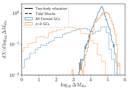
Figure 20: Integrated mass loss by disruption for all globular clusters observed at $z=0$ and all proto-GCs which form (including those which are disrupted by $z=0$). As is clear, the $z=0$ population of GCs have experienced much more mass loss through two-body relaxation than through tidal shocks. However, the population of all proto-GCs experience a nearly equal contribution from two-body relaxation and by tidal shocks. Omitting the effects of tidal shocks will result not only in more GCs surviving until $z=0$, but a different population of GCs compared to that which would be seen when including the effect of tidal shocks.

The effects of dynamical friction are also omitted from the LG1719 simulations, which is applied as a post-processing treatment in E-MOSAICS following Lacey & Cole (1993). Interestingly, despite the differences in both the formation model and the treatment of tidal disruption, both E-MOSAICS and LG1719 produce a similar final CMF, with an overabundance of low mass clusters. This suggests that the similar treatments of tidal disruption may need to be improved in the future to increase the disruption rate of low mass clusters. Despite the similarity in the CMFs in E-MOSAICS and LG1719, the metallicity distributions show opposite issues: too many metal-poor clusters in LG1719 and too many metal-rich clusters in E-MOSAICS. The different numerical approaches are the likely explanation of this. In E-MOSAICS, the ISM is under-resolved due to the fixed Jeans equation of state, leading to under-disruption in the metal-rich disc at lower redshifts (Kruijssen et al., 2019a). Meanwhile, in LG1719, tidal shocks are not included in the disruption rates, leading to under-disruption of globular clusters forming in high-redshift, low metallicity galaxies which experience frequent, violent mergers and inflow driven turbulence. With future improvements to the treatment of cold gas in E-MOSAICS and tidal disruption in LG1719, it is likely that both of these issues will be resolved and the results from the two simulation sets will further converge.

References

- Adamo et al. (2015) Adamo A., Kruijssen J. M. D., Bastian N., Silva-Villa E., Ryon J., 2015, MNRAS, 452, 246
- Agertz et al. (2013) Agertz O., Kravtsov A. V., Leitner S. N., Gnedin N. Y., 2013, ApJ, 770, 25
- Aguilar et al. (1988) Aguilar L., Hut P., Ostriker J. P., 1988, ApJ, 335, 720
- Ambartsumian (1938) Ambartsumian V. A., 1938, TsAGI Uchenye Zapiski, 22, 19
- Ashman & Zepf (1992) Ashman K. M., Zepf S. E., 1992, ApJ, 384, 50
- Bahé et al. (2017) Bahé Y. M., et al., 2017, MNRAS, 470, 4186
- Baldry et al. (2012) Baldry I. K., et al., 2012, MNRAS, 421, 621
- Barnes et al. (2017) Barnes D. J., et al., 2017, MNRAS, 471, 1088
- Bastian & Lardo (2018) Bastian N., Lardo C., 2018, ARAA, 56, 83
- Bastian et al. (2020) Bastian N., Pfeffer J., Kruijssen J. M. D., Crain R. A., Trujillo-Gomez S., Reina-Campos M., 2020, MNRAS submitted
- Baumgardt & Makino (2003) Baumgardt H., Makino J., 2003, MNRAS, 340, 227
- Baumgardt & Sollima (2017) Baumgardt H., Sollima S., 2017, MNRAS, 472, 744
- Baumgardt et al. (2008) Baumgardt H., De Marchi G., Kroupa P., 2008, ApJ, 685, 247
- Baumgardt et al. (2019) Baumgardt H., Hilker M., Sollima A., Bellini A., 2019, MNRAS, 482, 5138
- Beccari et al. (2010) Beccari G., Pasquato M., De Marchi G., Dalessand ro E., Trenti M., Gill M., 2010, ApJ, 713, 194
- Bedin et al. (2004) Bedin L. R., Piotto G., Anderson J., Cassisi S., King I. R., Momany Y., Carraro G., 2004, ApJ, 605, L125
- Behroozi et al. (2013) Behroozi P. S., Wechsler R. H., Conroy C., 2013, ApJ, 770, 57
- Bekki & Chiba (2002) Bekki K., Chiba M., 2002, ApJ, 566, 245
- Bekki et al. (2002) Bekki K., Forbes D. A., Beasley M. A., Couch W. J., 2002, MNRAS, 335, 1176
- Blakeslee et al. (1997) Blakeslee J. P., Tonry J. L., Metzger M. R., 1997, AJ, 114, 482
- Blom et al. (2012) Blom C., Spitler L. R., Forbes D. A., 2012, MNRAS, 420, 37
- Böker (2008) Böker T., 2008, ApJ, 672, L111
- Boylan-Kolchin (2018) Boylan-Kolchin M., 2018, MNRAS, 479, 332
- Brodie & Strader (2006) Brodie J. P., Strader J., 2006, ARAA, 44, 193
- Brooks et al. (2009) Brooks A. M., Governato F., Quinn T., Brook C. B., Wadsley J., 2009, ApJ, 694, 396
- Burkert & Forbes (2020) Burkert A., Forbes D. A., 2020, AJ, 159, 56
- Caldwell et al. (2011) Caldwell N., Schiavon R., Morrison H., Rose J. A., Harding P., 2011, AJ, 141, 61
- Carlberg (2020) Carlberg R. G., 2020, arXiv e-prints, p. arXiv:2001.00838
- Ceverino et al. (2010) Ceverino D., Dekel A., Bournaud F., 2010, MNRAS, 404, 2151
- Clowe et al. (2004) Clowe D., Gonzalez A., Markevitch M., 2004, ApJ, 604, 596
- Conroy & Gunn (2010) Conroy C., Gunn J. E., 2010, ApJ, 712, 833
- Conroy et al. (2011) Conroy C., Loeb A., Spergel D. N., 2011, ApJ, 741, 72
- Crain et al. (2015) Crain R. A., et al., 2015, MNRAS, 450, 1937
- Crain et al. (2017) Crain R. A., et al., 2017, MNRAS, 464, 4204
- De Rossi et al. (2017) De Rossi M. E., Bower R. G., Font A. S., Schaye J., Theuns T., 2017, MNRAS, 472, 3354
- Dekel & Birnboim (2006) Dekel A., Birnboim Y., 2006, MNRAS, 368, 2
- Djorgovski & Meylan (1994) Djorgovski S., Meylan G., 1994, AJ, 108, 1292
- Dolag et al. (2009) Dolag K., Borgani S., Murante G., Springel V., 2009, MNRAS, 399, 497
- Dotter et al. (2010) Dotter A., et al., 2010, ApJ, 708, 698
- Dotter et al. (2011) Dotter A., Sarajedini A., Anderson J., 2011, ApJ, 738, 74
- Efron (1979) Efron B., 1979, Ann. Statist., 7, 1
- Elmegreen (2010) Elmegreen B. G., 2010, ApJ, 712, L184
- Elmegreen & Hunter (2010) Elmegreen B. G., Hunter D. A., 2010, ApJ, 712, 604
- Erb et al. (2006) Erb D. K., Shapley A. E., Pettini M., Steidel C. C., Reddy N. A., Adelberger K. L., 2006, ApJ, 644, 813
- Fall & Rees (1985) Fall S. M., Rees M. J., 1985, ApJ, 298, 18
- Forbes & Bridges (2010) Forbes D. A., Bridges T., 2010, MNRAS, 404, 1203
- Forbes et al. (1997) Forbes D. A., Brodie J. P., Grillmair C. J., 1997, AJ, 113, 1652
- Forbes et al. (2018) Forbes D. A., et al., 2018, Proceedings of the Royal Society of London Series A, 474, 20170616
- Furlong et al. (2015) Furlong M., et al., 2015, MNRAS, 450, 4486
- Genel et al. (2009) Genel S., Genzel R., Bouché N., Naab T., Sternberg A., 2009, ApJ, 701, 2002
- Gensior et al. (2020) Gensior J., Kruijssen J. M. D., Keller B. W., 2020, arXiv e-prints, p. arXiv:2002.01484
- Genzel et al. (2011) Genzel R., et al., 2011, ApJ, 733, 101
- Gieles et al. (2006) Gieles M., Portegies Zwart S. F., Baumgardt H., Athanassoula E., Lamers H. J. G. L. M., Sipior M., Leenaarts J., 2006, MNRAS, 371, 793
- Gnedin (2003) Gnedin O. Y., 2003, ApJ, 582, 141
- Gnedin & Ostriker (1997) Gnedin O. Y., Ostriker J. P., 1997, ApJ, 474, 223
- Griffen et al. (2010) Griffen B. F., Drinkwater M. J., Thomas P. A., Helly J. C., Pimbblet K. A., 2010, MNRAS, 405, 375
- Haardt & Madau (2012) Haardt F., Madau P., 2012, ApJ, 746, 125
- Halbesma et al. (2019) Halbesma T. L. R., Grand R. J. J., Gómez F. A., Marinacci F., Pakmor R., Trick W. H., Busch P., White S. D. M., 2019, arXiv e-prints, p. arXiv:1909.02630
- Hansen et al. (2013) Hansen B. M. S., et al., 2013, Nature, 500, 51
- Harris (1996) Harris W. E., 1996, AJ, 112, 1487
- Harris (2016) Harris W. E., 2016, AJ, 151, 102
- Harris et al. (2017a) Harris W. E., Ciccone S. M., Eadie G. M., Gnedin O. Y., Geisler D., Rothberg B., Bailin J., 2017a, ApJ, 835, 101
- Harris et al. (2017b) Harris W. E., Blakeslee J. P., Harris G. L. H., 2017b, ApJ, 836, 67
- Hénon (1961) Hénon M., 1961, Annales d’Astrophysique, 24, 369
- Hernquist (1990) Hernquist L., 1990, ApJ, 356, 359
- Hopkins et al. (2012) Hopkins P. F., Quataert E., Murray N., 2012, MNRAS, 421, 3488
- Hopkins et al. (2014) Hopkins P. F., Kereš D., Oñorbe J., Faucher-Giguère C.-A., Quataert E., Murray N., Bullock J. S., 2014, MNRAS, 445, 581
- Hudson et al. (2015) Hudson M. J., et al., 2015, MNRAS, 447, 298
- Hughes et al. (2019) Hughes M. E., Pfeffer J., Martig M., Bastian N., Crain R. A., Kruijssen J. M. D., Reina-Campos M., 2019, MNRAS, 482, 2795
- Hughes et al. (2020) Hughes M. E., Pfeffer J. L., Martig M., Reina-Campos M., Bastian N., Crain R. A., Kruijssen J. M. D., 2020, MNRAS, 491, 4012
- Kamann et al. (2018) Kamann S., et al., 2018, MNRAS, 473, 5591
- Katz & White (1993) Katz N., White S. D. M., 1993, ApJ, 412, 455
- Kay et al. (2002) Kay S. T., Pearce F. R., Frenk C. S., Jenkins A., 2002, MNRAS, 330, 113
- Kennicutt (1998) Kennicutt Jr. R. C., 1998, ARAA, 36, 189
- Kim et al. (2018) Kim J.-h., et al., 2018, MNRAS, 474, 4232
- Kimm et al. (2016) Kimm T., Cen R., Rosdahl J., Yi S. K., 2016, ApJ, 823, 52
- Kravtsov & Gnedin (2005) Kravtsov A. V., Gnedin O. Y., 2005, ApJ, 623, 650
- Kravtsov et al. (1997) Kravtsov A. V., Klypin A. A., Khokhlov A. M., 1997, ApJS, 111, 73
- Kruijssen (2012) Kruijssen J. M. D., 2012, MNRAS, 426, 3008
- Kruijssen (2014) Kruijssen J. M. D., 2014, Classical and Quantum Gravity, 31, 244006
- Kruijssen (2015) Kruijssen J. M. D., 2015, MNRAS, 454, 1658
- Kruijssen et al. (2011) Kruijssen J. M. D., Pelupessy F. I., Lamers H. J. G. L. M., Portegies Zwart S. F., Icke V., 2011, MNRAS, 414, 1339
- Kruijssen et al. (2012) Kruijssen J. M. D., Pelupessy F. I., Lamers H. J. G. L. M., Portegies Zwart S. F., Bastian N., Icke V., 2012, MNRAS, 421, 1927
- Kruijssen et al. (2019a) Kruijssen J. M. D., Pfeffer J. L., Crain R. A., Bastian N., 2019a, MNRAS, 486, 3134
- Kruijssen et al. (2019b) Kruijssen J. M. D., Pfeffer J. L., Reina-Campos M., Crain R. A., Bastian N., 2019b, MNRAS, 486, 3180
- Kruijssen et al. (2020) Kruijssen J. M. D., et al., 2020, arXiv e-prints, p. arXiv:2003.01119
- Kundic & Ostriker (1995) Kundic T., Ostriker J. P., 1995, ApJ, 438, 702
- Lacey & Cole (1993) Lacey C., Cole S., 1993, MNRAS, 262, 627
- Lahén et al. (2020) Lahén N., Naab T., Johansson P. H., Elmegreen B., Hu C.-Y., Walch S., Steinwand el U. P., Moster B. P., 2020, ApJ, 891, 2
- Lamers et al. (2005) Lamers H. J. G. L. M., Gieles M., Portegies Zwart S. F., 2005, A&A, 429, 173
- Larsen et al. (2012) Larsen S. S., Strader J., Brodie J. P., 2012, A&A, 544, L14
- Leaman et al. (2013) Leaman R., VandenBerg D. A., Mendel J. T., 2013, MNRAS, 436, 122
- Lee & Ostriker (1987) Lee H. M., Ostriker J. P., 1987, ApJ, 322, 123
- Li & Gnedin (2019) Li H., Gnedin O. Y., 2019, MNRAS, 486, 4030
- Li et al. (2004) Li Y., Mac Low M.-M., Klessen R. S., 2004, ApJ, 614, L29
- Li et al. (2017) Li H., Gnedin O. Y., Gnedin N. Y., Meng X., Semenov V. A., Kravtsov A. V., 2017, ApJ, 834, 69
- Li et al. (2018) Li H., Gnedin O. Y., Gnedin N. Y., 2018, ApJ, 861, 107
- Ludlow et al. (2017) Ludlow A. D., et al., 2017, Physical Review Letters, 118, 161103
- Ma et al. (2016) Ma X., Hopkins P. F., Faucher-Giguère C.-A., Zolman N., Muratov A. L., Kereš D., Quataert E., 2016, MNRAS, 456, 2140
- Ma et al. (2020) Ma X., et al., 2020, MNRAS, 493, 4315
- Madau & Dickinson (2014) Madau P., Dickinson M., 2014, ARAA, 52, 415
- Madau et al. (2019) Madau P., Lupi A., Diemand J., Burkert A., Lin D. N. C., 2019, arXiv e-prints, p. arXiv:1905.08951
- Mandelker et al. (2018) Mandelker N., van Dokkum P. G., Brodie J. P., van den Bosch F. C., Ceverino D., 2018, ApJ, 861, 148
- Mannucci et al. (2009) Mannucci F., et al., 2009, MNRAS, 398, 1915
- Marín-Franch et al. (2009) Marín-Franch A., et al., 2009, ApJ, 694, 1498
- Miholics et al. (2017) Miholics M., Kruijssen J. M. D., Sills A., 2017, MNRAS, 470, 1421
- Moster et al. (2013) Moster B. P., Naab T., White S. D. M., 2013, MNRAS, 428, 3121
- Niederhofer et al. (2017) Niederhofer F., et al., 2017, MNRAS, 465, 4159
- Oppenheimer et al. (2016) Oppenheimer B. D., et al., 2016, MNRAS, 460, 2157
- Ostriker et al. (1972) Ostriker J. P., Spitzer Jr. L., Chevalier R. A., 1972, ApJ, 176, L51
- Peebles & Dicke (1968) Peebles P. J. E., Dicke R. H., 1968, ApJ, 154, 891
- Peng et al. (2006) Peng E. W., et al., 2006, ApJ, 639, 95
- Peng et al. (2008) Peng E. W., et al., 2008, ApJ, 681, 197
- Pfeffer et al. (2014) Pfeffer J., Griffen B. F., Baumgardt H., Hilker M., 2014, MNRAS, 444, 3670
- Pfeffer et al. (2018) Pfeffer J., Kruijssen J. M. D., Crain R. A., Bastian N., 2018, MNRAS, 475, 4309
- Pfeffer et al. (2019a) Pfeffer J., Bastian N., Crain R. A., Kruijssen J. M. D., Hughes M. E., Reina-Campos M., 2019a, MNRAS, 487, 4550
- Pfeffer et al. (2019b) Pfeffer J., Bastian N., Kruijssen J. M. D., Reina-Campos M., Crain R. A., Usher C., 2019b, MNRAS, 490, 1714
- Pontzen et al. (2013) Pontzen A., Roškar R., Stinson G., Woods R., 2013, pynbody: N-Body/SPH analysis for python, Astrophysics Source Code Library (ascl:1305.002)
- Portegies Zwart et al. (2010) Portegies Zwart S. F., McMillan S. L. W., Gieles M., 2010, ARAA, 48, 431
- Pozzetti et al. (2019) Pozzetti L., Maraston C., Renzini A., 2019, MNRAS, 485, 5861
- Prieto & Gnedin (2008) Prieto J. L., Gnedin O. Y., 2008, ApJ, 689, 919
- Puzia et al. (2005) Puzia T. H., Kissler-Patig M., Thomas D., Maraston C., Saglia R. P., Bender R., Goudfrooij P., Hempel M., 2005, A&A, 439, 997
- Qu et al. (2017) Qu Y., et al., 2017, MNRAS, 464, 1659
- Ramos-Almendares et al. (2019) Ramos-Almendares F., Sales L. V., Abadi M. G., Doppel J. E., Muriel H., Peng E. W., 2019, arXiv e-prints, p. arXiv:1906.11921
- Reina-Campos & Kruijssen (2017) Reina-Campos M., Kruijssen J. M. D., 2017, MNRAS, 469, 1282
- Reina-Campos et al. (2018) Reina-Campos M., Kruijssen J. M. D., Pfeffer J., Bastian N., Crain R. A., 2018, MNRAS, 481, 2851
- Reina-Campos et al. (2019) Reina-Campos M., Kruijssen J. M. D., Pfeffer J. L., Bastian N., Crain R. A., 2019, MNRAS, 486, 5838
- Reina-Campos et al. (2020) Reina-Campos M., Hughes M. E., Kruijssen J. M. D., Pfeffer J. L., Bastian N., Crain R. A., Koch A., Grebel E. K., 2020, MNRAS, 493, 3422
- Renaud et al. (2017) Renaud F., Agertz O., Gieles M., 2017, MNRAS, 465, 3622
- Renzini (2017) Renzini A., 2017, MNRAS, 469, L63
- Renzini et al. (2015) Renzini A., et al., 2015, MNRAS, 454, 4197
- Sarajedini et al. (2007) Sarajedini A., et al., 2007, AJ, 133, 1658
- Sawala et al. (2016) Sawala T., et al., 2016, MNRAS, 457, 1931
- Schaller et al. (2015) Schaller M., Dalla Vecchia C., Schaye J., Bower R. G., Theuns T., Crain R. A., Furlong M., McCarthy I. G., 2015, MNRAS, 454, 2277
- Schaye (2004) Schaye J., 2004, ApJ, 609, 667
- Schaye et al. (2015) Schaye J., et al., 2015, MNRAS, 446, 521
- Schechter (1976) Schechter P., 1976, ApJ, 203, 297
- Smith (1999) Smith G. H., 1999, ApJ, 526, L21
- Sollima & Baumgardt (2017) Sollima A., Baumgardt H., 2017, MNRAS, 471, 3668
- Spitler & Forbes (2009) Spitler L. R., Forbes D. A., 2009, MNRAS, 392, L1
- Spitzer (1940) Spitzer Lyman J., 1940, MNRAS, 100, 396
- Spitzer & Harm (1958) Spitzer Jr. L., Harm R., 1958, ApJ, 127, 544
- Springel et al. (2001) Springel V., Yoshida N., White S. D. M., 2001, New Astron., 6, 79
- Tacconi et al. (2013) Tacconi L. J., et al., 2013, ApJ, 768, 74
- Tremaine (1976) Tremaine S. D., 1976, ApJ, 203, 72
- Trenti et al. (2015) Trenti M., Padoan P., Jimenez R., 2015, ApJ, 808, L35
- Turner et al. (2017) Turner M. L., Schaye J., Crain R. A., Rudie G., Steidel C. C., Strom A., Theuns T., 2017, MNRAS, 471, 690
- Usher et al. (2012) Usher C., et al., 2012, MNRAS, 426, 1475
- Usher et al. (2018) Usher C., Pfeffer J., Bastian N., Kruijssen J. M. D., Crain R. A., Reina-Campos M., 2018, MNRAS, 480, 3279
- Usher et al. (2019) Usher C., Brodie J. P., Forbes D. A., Romanowsky A. J., Strader J., Pfeffer J., Bastian N., 2019, MNRAS, 490, 491
- VandenBerg et al. (2013) VandenBerg D. A., Brogaard K., Leaman R., Casagrande L., 2013, ApJ, 775, 134
- Watkins et al. (2015) Watkins L. L., van der Marel R. P., Bellini A., Anderson J., 2015, ApJ, 812, 149
- Webb & Leigh (2015) Webb J. J., Leigh N. W. C., 2015, MNRAS, 453, 3278
- Webb et al. (2017) Webb J. J., Vesperini E., Dalessandro E., Beccari G., Ferraro F. R., Lanzoni B., 2017, MNRAS, 471, 3845
- Wiersma et al. (2009) Wiersma R. P. C., Schaye J., Theuns T., Dalla Vecchia C., Tornatore L., 2009, MNRAS, 399, 574
- Woods et al. (2014) Woods R. M., Wadsley J., Couchman H. M. P., Stinson G., Shen S., 2014, MNRAS, 442, 732
- Zinn (1985) Zinn R., 1985, ApJ, 293, 424
- Zinnecker et al. (1988) Zinnecker H., Keable C. J., Dunlop J. S., Cannon R. D., Griffiths W. K., 1988, in Grindlay J. E., Philip A. G. D., eds, IAU Symposium Vol. 126, The Harlow-Shapley Symposium on Globular Cluster Systems in Galaxies. p. 603