Daniel R. Chavas \extraaffilPurdue University, Department of Earth, Atmospheric, and Planetary Sciences, West Lafayette, IN \extraauthorKevin A. Reed \extraaffilSchool of Marine and Atmospheric Sciences, Stony Brook University, Stony Brook, NY \extraauthor Daniel T. Dawson II \extraaffilPurdue University, Department of Earth, Atmospheric, and Planetary Sciences, West Lafayette, IN
Climatology of severe local storm environments and synoptic-scale features over North America in ERA5 reanalysis and CAM6 simulation
Abstract
Severe local storm (SLS) activity is known to occur within specific thermodynamic and kinematic environments. These environments are commonly associated with key synoptic-scale features–including southerly Great Plains low-level jets, drylines, elevated mixed layers, and extratropical cyclones–that link the large-scale climate to SLS environments. This work analyzes spatiotemporal distributions of both the environmental parameters and synoptic-scale features in ERA5 reanalysis and in Community Atmosphere Model version 6 (CAM6) during 1980–2014 over North America. Compared to radiosondes, ERA5 successfully reproduces SLS environments, with strong spatiotemporal correlations and low biases, especially over the Great Plains. Both ERA5 and CAM6 reproduce the climatology of SLS environments over the central United States as well as its strong seasonal and diurnal cycles. ERA5 and CAM6 also reproduce the climatological occurrence of the synoptic-scale features, with the distribution pattern similar to that of SLS environments. Compared to ERA5, CAM6 exhibits a high bias in Convective Available Potential Energy over the eastern United States primarily due to a high bias in surface moisture, and to a lesser extent, storm-relative helicity due to enhanced low-level winds. Composite analysis indicates consistent synoptic anomaly patterns favorable for significant SLS environments over much of the eastern half of the United States in both ERA5 and CAM6, though the pattern differs for the southeastern United States. Overall, results indicate that both ERA5 and CAM6 are capable of reproducing SLS environments as well as the synoptic-scale features and transient events that generate them.
1 Introduction
Severe local storm (SLS) environments are favorable atmospheric conditions for the development of SLS events, including severe thunderstorms accompanied by damaging winds, large hailstones, and/or tornadoes (Ludlam 1963; Johns and Doswell III 1992). Such environments are commonly defined by high values of a small number of key thermodynamic and kinematic parameters: convective available potential energy (CAPE), lower-tropospheric (0–6-km) bulk vertical wind shear (S06), and 0–3-km storm-relative helicity (SRH03) (Rasmussen and Blanchard 1998; Rasmussen 2003; Brooks et al. 2003; Doswell III and Schultz 2006; Grams et al. 2012). CAPE is the vertical integral of buoyancy from the level of free convection to the equilibrium level and thus provides a measure of conditional instability for a potential storm (Doswell III and Rasmussen 1994). Given the standard assumptions of parcel theory, CAPE is proportional to the theoretical maximum updraft wind speed (Holton 1973). S06 and SRH03 are proxies of environmental crosswise and streamwise vorticity available to generate updraft rotation (Rotunno and Klemp 1982, 1985; Davies-Jones et al. 1990; Davies-Jones 1993; Weisman and Rotunno 2000; Davies-Jones 2002; Rotunno and Weisman 2003; Davies-Jones 2003). These conditions work in combination to permit the generation of persistent rotating updrafts that are the defining characteristic of supercell storms (Doswell III and Burgess 1993). Given that both thermodynamic and kinematic “ingredients” are necessary, composite proxies, such as the product of CAPE and S06 (CAPES06) and the energy helicity index (EHI03; proportional to the product of CAPE and SRH03), are commonly employed as representative measures of the SLS potential of a given environment (Davies-Jones 1993; Brooks et al. 2003; Thompson et al. 2003). Composite proxies are in general preferable to the constituent parameters alone in discriminating conducive environments for SLS events (Rasmussen and Blanchard 1998; Brooks et al. 2003), while the individual constituent parameters are indicative of the key underlying physical processes (Doswell III and Schultz 2006).
The generation of SLS environments depends on synoptic-scale features that serve as an intermediate-scale bridge between weather and climate scales. Over the Great Plains of North America, the generation of SLS environments is intimately associated with the southerly Great Plains low-level jets, drylines, elevated mixed layers, and extratropical cyclones. The southerly Great Plains low-level jets (GPLLJs), defined by the low-level maximum winds, commonly form during the nighttime (Bonner 1968; Whiteman et al. 1997). GPLLJs modulate Great Plains precipitation (Weaver and Nigam 2008) and its moisture budget by transporting almost one-third of the moisture that enters the contiguous United States (Helfand and Schubert 1995), which is an important contributor to the formation of high-CAPE environments (Helfand and Schubert 1995; Higgins et al. 1997; Weaver et al. 2012). Drylines and elevated mixed layers (EMLs) are associated with the eastward advection of well-mixed air with relatively high potential temperature generated by strong surface heating over the elevated dry deserts of the Mexican Plateau. Meridionally oriented drylines are common across the central and southern Great Plains when this dry airmass from the west encounters the moist near-surface airmass advected northward from the Gulf of Mexico (Fujita 1958; Schaefer 1974; Ziegler and Hane 1993; Hoch and Markowski 2005), producing a focused linear band of convergence and moisture gradients (Rhea 1966; Ziegler and Rasmussen 1998; Xue and Martin 2006; Schultz et al. 2007). The advection of the well-mixed layer atop the low-level moist air generates the EML, often creating a strong capping inversion at the base of the EML (Carlson et al. 1983; Lanicci and Warner 1991a; Banacos and Ekster 2010). Subsequent daytime heating of the moist boundary layer allows for the removal of convective inhibition and a strong buildup of CAPE (Carlson et al. 1983; Farrell and Carlson 1989; Lanicci and Warner 1991b, c; Cordeira et al. 2017). Extratropical cyclones strongly enhance low-level moisture and heat convergence within their warm sectors, thereby enhancing CAPE (Hamill et al. 2005; Tochimoto and Niino 2015). Moreover, the cyclonic circulation itself and the baroclinic instability linked to the evolution of extratropical cyclones via thermal wind balance also act to enhance the vertical wind shear (Doswell III and Bosart 2001).
Previous studies have documented the climatological variability, including the amplitude and spatial pattern, of the SLS environmental proxies and parameters (Brooks et al. 2003; Wagner et al. 2008; Gensini and Ashley 2011; Diffenbaugh et al. 2013; Tippett et al. 2015; Gensini and Brooks 2018; Gensini and Bravo de Guenni 2019; Tang et al. 2019), as well as the key synoptic-scale features that help generate these environments (Bonner 1968; Reitan 1974; Zishka and Smith 1980; Lanicci and Warner 1991a; Whiteman et al. 1997; Hoch and Markowski 2005; Duell and Van Den Broeke 2016; Ribeiro and Bosart 2018). It is known from these studies that the SLS environments and the associated synoptic-scale features have strong seasonal and diurnal cycles, which emphasizes the influence of variations in the fundamental types of external climate forcing (earth orbit and solar insolation). However, these studies have analyzed different geographic domains and time-periods using different datasets, which makes holistic analysis and inter-comparison difficult.
Reanalysis datasets, combining multi-source observations and model-based forecasts via advanced data assimilation methods, provide a synthesized representation of the atmosphere over long historical time periods and thus have become an indispensable data source for the study of weather and climate from synoptic to planetary scales. Several reanalysis datasets have been used to investigate the climatological distribution or variation of SLS environments, including NCEP/NCAR (Brooks et al. 2003; Diffenbaugh et al. 2013), North American Regional Reanalysis (NARR) (Gensini and Ashley 2011; Gensini et al. 2014a; Tippett et al. 2016; Gensini and Brooks 2018; Tang et al. 2019), and ERA-Interim (Allen and Karoly 2014; Taszarek et al. 2018). These reanalyses in general produce similar spatial patterns but slightly different magnitudes for the climatology of SLS environments. Recent work evaluated the performance of ERA-Interim and NARR in estimating the environmental proxies and parameters by comparing them with radiosonde measurements (Gensini et al. 2014a; Taszarek et al. 2018), indicating that these reanalyses reproduce the observed spatial and temporal trends of SLS environments, though they exhibit larger regional biases in thermodynamic parameters (e.g., CAPE) than in kinematic parameters (e.g., S06). In addition, these reanalyses in general produce lower biases over flat terrain than in coastal areas and mountains owing to the limited horizontal resolution and sharp variations of atmospheric variables across regions with complex topography (Taszarek et al. 2018). Thus, caution is needed when interpreting results from reanalysis datasets considering the various uncertainties associated with the measurements and forecasts incorporated, as well as the complex inferential process that involves data assimilation for generating reanalysis datasets (Parker 2016). Such evaluation is necessary for identifying potential strengths and limitations of a reanalysis dataset for studying SLS environments (Gensini et al. 2014a) and a higher-resolution reanalysis dataset is expected to better represent these atmospheric environments.
Additionally, global climate models have been a useful tool to study SLS environments (Tippett et al. 2015). As with reanalyses, such models are too low-resolution to resolve actual SLS events, but they are capable of resolving larger-scale SLS environments. Though climate models do not reproduce the day-to-day weather, they are able to capture the statistical behavior of the present-day climate. Thereby, climate models have been widely used to analyze SLS environments in current or future climate simulations to assess the impacts of climate changes on SLS activity, assuming that changes in SLS activity will follow changes in the statistics of SLS environments (Trapp et al. 2007; Diffenbaugh et al. 2013; Romps et al. 2014; Seeley and Romps 2015; Tippett et al. 2016; Gensini and Brooks 2018). These models in general reproduce reasonable historical climatologies of SLS environments, though biases vary across models when compared to the reanalysis- or radiosonde-based climatology (Diffenbaugh et al. 2013; Seeley and Romps 2015). Forced with coarse-resolution output from global climate models, dynamical downscaling through high-resolution regional climate models has shown substantial potential for assessment of both SLS events and environments (Trapp et al. 2011; Robinson et al. 2013; Gensini and Mote 2014, 2015; Hoogewind et al. 2017).
The purpose of this study is therefore to evaluate the representations of both SLS environments and synoptic-scale features commonly associated with the generation of these environments over North America in a new high-resolution global reanalysis dataset (ERA5) and a climate model (the Community Atmosphere Model version 6, CAM6). A comprehensive analysis and comparison of the climatologies of these environments and the synoptic-scale features provides an important reference for using reanalyses and climate models to better understand climate controls on SLS activities in any climate state.
This work addresses the following questions:
-
1.
How well does the ERA5 reanalysis represent the observed climatology of SLS environments over the contiguous United States?
-
2.
How does this climatology, including seasonal and diurnal cycles, compare between the ERA5 reanalysis and CAM6 simulation?
-
3.
What are the climatological distributions of the key synoptic-scale features commonly associated with the generation of SLS environments over North America in the ERA5 reanalysis and CAM6 simulation?
-
4.
What are the characteristic synoptic patterns associated with SLS environments in the ERA5 reanalysis and CAM6 simulation? Do they vary from region to region?
To answer these questions, we first compare SLS environments between the ERA5 reanalysis and radiosonde observations. This examines the ability of the ERA5 reanalysis in reproducing both statistical property of the present-day climate and the observed day-to-day weather in terms of SLS environments. As climate models simulate climate statistics, we then compare the climatology, including seasonal and diurnal cycles, of extreme SLS environments and the associated synoptic-scale features between the ERA5 reanalysis and CAM6 simulation, as well as analyze biases in the CAM6 simulation. Finally, we create and compare synoptic composites associated with extreme SLS environments within a set of predefined regions across the eastern half of the United States to analyze the extent to which CAM6 reproduces the characteristic synoptic-scale flow patterns that generate these events across regions.
Section 2 introduced the data, experimental design, and our analysis methodology. We evaluate the ERA5 reanalysis against radiosonde observations in Section 3. Section 4 presents climatologies of SLS environments and synoptic-scale features, and synoptic composites. Finally, we provide conclusions and discussion of results and future work in Section 5.
2 Methodology
2.1 Datasets
We use radiosonde observations for the period 1998–2014, and the ERA5 reanalysis and CAM6 historical simulation data each for the period 1980–2014. The radiosonde observations are first used to evaluate the representation of SLS environments in ERA5 over the contiguous United States. Then, the CAM6 simulation is compared in-depth to ERA5 for North America. Each data source is described in detail below.
2.1.1 Observation: Radiosonde
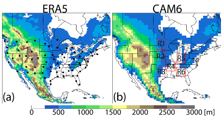
Radiosonde observations are obtained from the sounding database of the University of Wyoming (http://weather.uwyo.edu/upperair/sounding.html). This dataset includes 69 radiosonde stations over the contiguous United States with twice-daily raw soundings at 0000 and 1200 UTC. Three stations (the KUNR station over western South Dakota, the KVEF station over southern Nevada, and the KEYW station on the island of Key West) are excluded in this study because of a lack of multi-year records, resulting in 66 stations (Figure 1a). Roughly half of the radiosonde stations from the database do not have records before around 1994 and most stations were moved 0.01–0.03 degree along the longitude or latitude in 1990’s (in or before 1997) due to the National Weather Service modernization. Thus, we only use radiosonde observations for the period 1998–2014 in this work, similar to Gensini et al. (2014a). Furthermore, we apply the following quality-control checks to each sounding before use: (1) height and pressure arrays are in correct order: height increases and pressure decreases with time; (2) wind speed 0 kts, 0∘ wind direction 360∘, and temperature and dewpoint temperature 0 K; (3) height of the first record equals the local elevation; (4) top height 6 km and top pressure 100 hPa; and (5) the maximum pressure decrease between consecutive records 50 hPa. The first two checks follow the quality control done in SHARPpy (Blumberg et al. 2017); the third check ensures that the ground surface observation is available for calculating the surface-based CAPE; the fourth and fifth checks ensure that the vertical resolution of the sounding is identical with or higher than the ERA5 reanalysis, as the purpose of using radiosondes is to evaluate the ERA5 representations. The number percentage of qualified records for each radiosonde station is over 60% (Figure S1a).
2.1.2 Reanalysis: ERA5
The fifth generation of the European Centre for Medium-Range Weather Forecasts (ECMWF) global climate reanalysis, ERA5, spans the period 1979–present (Hersbach and Dee 2016). Here we use years 1980–2014, downloaded from NCAR’s Research Data Archive (date accessed: 09-19-2019; ECMWF 2019), for direct comparison with radiosondes and climate model simulation (described below). The dataset provides hourly variables at or near the surface and 37 constant pressure levels from 1000–1 hPa. These pressure-level data are produced by interpolating from the ECMWF’s Integrated Forecast System with 137 hybrid sigma-pressure model levels in the vertical, up to a top level of 0.01 hPa (Hersbach and Dee 2016); this reduction of vertical resolution may induce errors to calculations of vertically integrated parameters, such as CAPE and SRH03 (defined below). The horizontal grid spacing of ERA5 is 0.25 degree (roughly 31 km), which is higher than its predecessor ERA-Interim (79 km; Dee et al. 2011). Other improvements in ERA5 include using a revised data assimilation system and improved core dynamics and model physics (Hersbach and Dee 2016).
2.1.3 Modeling: CAM6
The Community Atmosphere Model version 6 (CAM6) is used for the simulation portion of this work. CAM6 is the atmospheric component of the Community Earth System Model version 2.1 ( available at http://www.cesm.ucar.edu/models/cesm2/) developed in part for participation in the Coupled Model Intercomparison Project 6 (CMIP6; Eyring et al. 2016). CAM6 builds off its predecessor CAM5 (documented in detail in Neale et al. 2012) with significant modifications to the physical parameterization suite. In particular, CAM5 schemes for cloud macrophysics, boundary layer turbulence and shallow convection have been replaced by the Cloud Layers Unified by Binormals (CLUBB; Golaz et al. 2002; Bogenschutz et al. 2013) scheme. In addition, CAM6 now implements the two-moment prognostic cloud microphysics from Gettelman and Morrison (2015), as well as additional updates to the Zhang and McFarlane (1995) deep convection and orographic drag parameterizations. CAM6 is configured with the default finite volume dynamical core on a 0.91.25∘ latitude-longitude grid mesh with 32 hybrid sigma-pressure levels. Our CAM6 simulation is configured as a historical simulation following Atmospheric Model Intercomparison protocols (Gates et al. 1999) over the period 1979–2014. We discard the first year for spinup and analyze the 3-hourly output from 1980–2014 for direct comparison with ERA5 reanalysis.
2.2 Analysis
We perform a climatological analysis of: (1) the annual, seasonal, and diurnal distributions of significant SLS environmental proxies and their constituent parameters (defined below); (2) the occurrence frequency distributions of key synoptic-scale features: southerly Great Plains low-level jets, drylines, elevated mixed layers, and extratropical cyclone activity over North America; and (3) characteristic synoptic composites associated with extreme SLS environments in different geographic regions over the eastern half of the United States. To evaluate ERA5 performance using radiosondes, we extract ERA5 at 0000 and 1200 UTC for 1998–2014, consistent with the radiosonde temporal resolution and coverage, and then linearly interpolate ERA5 results onto the radiosonde sites. To compare simulation with reanalysis, calculations for ERA5 and CAM6 are all done for 3-hourly outputs from 1980–2014 and then linearly interpolated onto 1∘1∘ grids. These horizontally linear interpolations are performed via the function of in the open-source matplotlib Python package (Hunter 2007).
2.2.1 SLS Environments
SLS Environmental Proxies and Parameters: We calculate two combined proxies, CAPES06 and EHI03, to represent SLS environments. CAPES06 (Brooks et al. 2003) and EHI03 (Hart and Korotky 1991; Davies-Jones 1993) are calculated by
| (1) |
and
| (2) |
respectively. As for each constituent parameter, CAPE is defined as (Doswell III and Rasmussen 1994):
| (3) |
where 9.81 m s-2 is the acceleration due to gravity, denotes the level of free convection, denotes the equilibrium level, and and is the virtual temperature of the 2-m parcel and the environment. Here we select the 2-m parcel for simplicity its consistent availability across all our datasets; it also avoids biases in defining other types of parcels (e.g., most-unstable or mixed-layer parcel) associated with differences in the vertical resolutions of the datasets. S06 is defined as the magnitude difference of wind vectors at 6 km and 10 m above the surface (Rasmussen and Blanchard 1998; Weisman and Rotunno 2000). SRH03 is defined as (Davies-Jones et al. 1990)
| (4) |
where V is horizontal wind vector, C is the storm motion vector following the definition and calculation from Bunkers et al. (2000), m is the altitude of the layer bottom, km is the altitude of the layer top, and is the vertical unit vector. We create the climatologies of SLS environments using CAPES06 and EHI03, respectively, as well as their constituent parameters (CAPE, S06, and SRH03).
Analysis of Extremes: We define “significant” (or “extreme”) SLS environments using the 99th percentile of the proxies and parameters, similar to past work (Tippett et al. 2016; Singh et al. 2017). The 99th percentile is calculated for each station site (for radiosondes) or each grid point (for ERA5 reanalysis or CAM6 simulation) based on the full-period (1998–2014 or 1980–2014) time series of each variable at the location. We also analyzed the 95th, 90th, and 75th percentiles, and found qualitatively similar climatological patterns across these high percentiles (analyzed below in Figure S4).
2.2.2 SLS-relevant synoptic-scale features
Southerly Great Plains Low-Level Jet (GPLLJ): We follow Bonner (1968) and Whiteman et al. (1997) to identify low level jets (LLJs). The method detects LLJs and defines an intensity category 0–3 based on two criteria: (1) the maximum wind speed below 3000 m: 10, 12, 16, or 20 m s-1 and (2) the largest decrease from in the layer from the height of to 3000 m: 5, 6, 8, or 10 m s-1. To identify specifically southerly LLJs, each detected LLJ is further classified as southerly if the direction of falls between 113∘ and 247∘, and as northerly if between 293∘ and 67∘ following Walters et al. (2008) and Doubler et al. (2015). Using these category- and direction-based criteria, we successfully detect various LLJs over North America, including the southerly and northerly GPLLJ, the northerly Pacific coast LLJ, the northerly Tehuantepec LLJ, and the easterly Caribbean LLJ, as documented in Doubler et al. (2015). The climatology of southerly GPLLJ in category 0 ( 10 m s-1 and 5 m s-1) is presented in this work.
Dryline: Drylines are identified at each grid point following the criteria in Duell and Van Den Broeke (2016): (1) the horizontal gradient of the surface specific humidity is at least 0.03 g kg-1 km-1 and the specific humidity gradient from west to east must be positive, (2) the surface temperature gradient from west to east is less than 0.02 K km-1, and (3) a surface wind shift exists with wind direction on the west side being between 170∘ and 280∘, and on the east side being between 80∘ and 190∘. The first criterion is consistent with the approach of Hoch and Markowski (2005), in which the specific humidity gradient is recommended instead of the dewpoint temperature gradient as the specific humidity is less sensitive to the varying elevation. The other two criteria are used in an effort to differentiate drylines from cold fronts. The limitations of the algorithm are further discussed in Duell and Van Den Broeke (2016).
Elevated Mixed Layer (EML): An EML is identified for a sounding that satisfies the following criteria, based on Banacos and Ekster (2010) and Ribeiro and Bosart (2018): (1) a candidate EML is identified as a layer with lapse rate equal to or greater than 8.0 K km-1 through a depth of at least 200 hPa, (2) the environmental relative humidity increases from the base to the top of the candidate EML, (3) the base of the candidate EML is at least 1000 m above the surface but below the 500-hPa level, and (4) the average lapse rate between the base and the surface is less than 8.0 K km-1. Here, the EML base is defined as the first model level from the bottom with lapse rate equal to or greater than 8.0 K km-1. The third and fourth criteria ensure the exclusion of surface-based or upper-tropospheric mixed layers.
Extratropical Cyclone Activity: Extratropical cyclone activity is defined using two methods: (1) cyclone track frequency calculated from explicit tracking of cyclone centers, and (2) eddy kinetic energy (EKE), which captures the spatial distribution of eddy activity in general.
The open-source TempestExtremes tracking algorithm (Ullrich and Zarzycki 2017) is used to detect and track individual extratropical cyclones using similar criteria described in Zarzycki (2018). Candidate cyclones are determined by searching for minima in sea level pressure with a closed contour of 2 hPa within 6 great circle degrees of the minimum. Candidate cyclones, which are detected at 3-hourly increments, are then stitched together in time by searching within an 8-degree great circle radius at the next time increment for another candidate cyclone to form a cyclone track. For a cyclone track to be included in the analysis it must exist for at least 9 time slices representing a minimum cyclone track length of 24 hours.
EKE at 850 hPa is calculated by
| (5) |
where represent zonal and meridional velocity deviations from the annual mean velocities that obtained by averaging the velocities over the entire study period (1980–2014). Calculating with respect to a multi-year, or yearly, or moving seasonal average does not change the amplitude or phase of the seasonal cycle of EKE significantly (Rieck et al. 2015). Following past work (Blackmon 1976; Ulbrich et al. 2008; Harvey et al. 2014; Schemm and Schneider 2018), we apply a 2–6-day Butterworth bandpass filter (Russell 2006) to to retain reasonable timescales of extratropical cyclone activities. Other bandpass ranges, such as 2–8-day (Yin 2005) and 3–10-day (Kaspi and Schneider 2013; Tamarin and Kaspi 2016), are also tested. EKE is quantitatively sensitive to the bandpass range: longer range (e.g., 2–8-day vs. 2–6-day) translates to larger EKE, but the qualitative spatial pattern and seasonal variation of EKE are not sensitive to these ranges (not shown).
2.2.3 Synoptic Composites for Extreme Cases
We calculate the composite of synoptic anomalies conditioned on extreme SLS environments within six 5∘ regions (i.e., R1–R6 in Figure 1b) from ERA5 and CAM6. R2–R4 are selected following Ribeiro and Bosart (2018); we also select sub-regions over the northern Great Plains (R1), the Midwest (R5), and the southeastern United States (R6), so that our analysis spans much of the land east of the Rocky Mountains where SLS activity and environments are concentrated. In this study, we define an extreme case in a region when the CAPES06 exceeds its local 99th percentile (i.e., within the top 1%) in at least 80% of the total grid points within the region. To generate the composite synoptic anomalies for each region, we first calculate the synoptic anomalies of each case from the full-period (1980–2014) monthly mean state (e.g., for a case selected in July 2012, the anomaly field of a variable is the difference between the variable field from the case and the mean field of the variable during 1980-2014 in July). Then, we generate composite synoptic anomalies at 250 hPa (horizontal winds and geopotential height), 700 hPa (horizontal winds, temperature, and geopotential height), and surface (10-m winds, 2-m specific humidity, and sea level pressure) by averaging the anomaly fields of the extreme cases for each region. The composite synoptic patterns based on a 50% threshold is qualitatively similar, though with less distinctive features (e.g., a smoothed trough or wind fields; not shown). The 50% threshold produces more candidates for each region than the 80% threshold does, but also introduces larger variance that may reduce similarity across cases.
3 Results: Radiosonde and ERA5
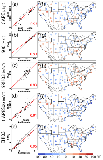
We begin by comparing the extreme values (99th percentile) of SLS environmental parameters and proxies in the ERA5 reanalysis against radiosondes to investigate the extent to which the ERA5 reanalysis can reproduce the observed SLS environments. We first calculate the pattern correlation coefficient between ERA5 and radiosondes, as well as the bias (defined as percentage difference from radiosonde value) in ERA5 for each parameter and proxy (Figure 2). ERA5 in general performs well in reproducing extreme values of these constituent parameters, with strong pattern correlation (CAPE: 0.93; S06: 0.93; SRH03: 0.83; Figure 2a–c) and relatively low bias, especially over the Great Plains ( 10%; Figure 2f–h). Specifically, extreme CAPE is generally underestimated (-10%–0 for the central Great Plains; -40%– -10% for other areas) for most stations east of the Rocky Mountains and overestimated ( 40%) over high terrains to the west (Figure 2f); extreme S06 has the smallest bias (within 10%) across most stations (Figure 2g); extreme SRH03 is generally underestimated over central and western United States with relatively low bias over the Great Plains (within 10%), while overestimated over eastern United States (10%–40%; Figure 2h). Owing to the strong pattern correlations in these constituent parameters, the combined proxies, CAPES06 and EHI03, also have strong pattern correlations (CAPES06: 0.91; EHI03: 0.95), though they are in general underestimated by ERA5 (Figure 2d, e). Biases of extreme CAPES06 is similar to the biases of extreme CAPE; biases of extreme EHI03 are slightly enhanced due to the combined influence of the constituent parameters, with negative bias of generally -40% – -10% across most stations over the central United States and -80% – -40% over western and northeastern United States (Figure 2i, j).
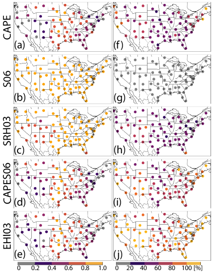
Similar good performance is found for the full-period (1998–2014) time series of each parameter and proxy at each station in terms of the temporal correlation (Figure 3a–e) and root-mean-square error (RMSE; Figure 3f–j). Here we condition the radiosondes on CAPE 500 J kg-1, as our focus is on the environments that could support SLS events. This threshold is only applied to CAPE (and thus CAPES06 and SRH03), resulting in a smaller sample size at each site for these parameters (Figure S1c) than for S06 and SRH03 (Figure S1a). ERA5 has relatively strong temporal correlations ( 0.8) and small RMSEs ( 40%) for CAPE over the Great Plains and the Midwest as compared to other areas (Figure 3a,f), and does an excellent job in representing S06 at all sites (temporal correlation 0.8; RMSE 20%; Figure 3b,g) and SRH03 over eastern half of the United States (temporal correlation 0.8; 40% RMSE 60%; Figure 3c,h). Regarding CAPES06 (Figure 3d,i) and EHI03 (Figure 3e,j), stations over the Great Plains in general have strong temporal correlation (0.8) and relatively low RMSE (CAPES06: 40%–60%; EHI03: 60%–80% ) as compared to the western United States and eastern coastal areas. Additionally, we perform similar analyses but condition CAPE, CAPES06, and EHI03 on CAPE 0 J kg-1, as SLS events also occur within low-CAPE environments (e.g., the SLS activity commonly associated with low-CAPE, high-shear environments over the Southeast). By including these low-CAPE cases, both the temporal correlations and RMSEs of CAPE, CAPES06, and EHI03 increase (Figure S2), indicating persistent and relatively large biases for the low-CAPE cases. Note though that including cases with CAPE below 500 J kg-1 skews the majority of our dataset to these relatively low CAPE values and so is much less representative of significant SLS environments over Great Plains.
Overall, ERA5 performs reasonably well in reproducing the spatiotemporal variability of key SLS environmental parameters and proxies when compared against radiosonde data, particularly east of the Rocky Mountains where SLS activity is most common. Kinematic parameters (S06 and SRH03) are generally better estimated than thermodynamic parameters (CAPE) by the ERA5 reanalysis, particularly in the mountain west and eastern coasts, due to resolution limitations and associated intrinsic difficulties representing thermodynamic variability in complex terrains (Taszarek et al. 2018). This is similar to the performance of other reanalyses (Gensini et al. 2014a; Taszarek et al. 2018). The temporal analyses (Figure 3) indicate that there may be significant errors in the values of SLS environmental parameters and proxies at any given point in time at a given location. However, for climatological studies such as this work, it is the high percentiles (Figure 2) that are most important to adequately represent.
4 Results: ERA5 and CAM6
We now move on to an in-depth analysis of significant SLS environments and the associated synoptic-scale features over North America in both ERA5 reanalysis dataset and CAM6 simulation for period 1980–2014. Since the ERA5 reasonably reproduces SLS environments, based on its strong spatiotemporal correlations and relatively small biases with respect to radiosonde observations, especially over much of the eastern half of the United States where SLS activity is most prominent, this allows for an assessment of how CAM6 reproduces these climatological environments and the associated synoptic-scale features over North America as compared to the ERA5. Biases in CAM6 simulation with respect to the ERA5 are analyzed in terms of biases in the mean-state atmosphere. Additionally, common synoptic patterns that favor extreme SLS environments in regions east of the Rocky Mountains are analyzed.
4.1 SLS Environments
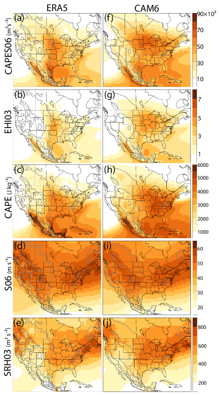
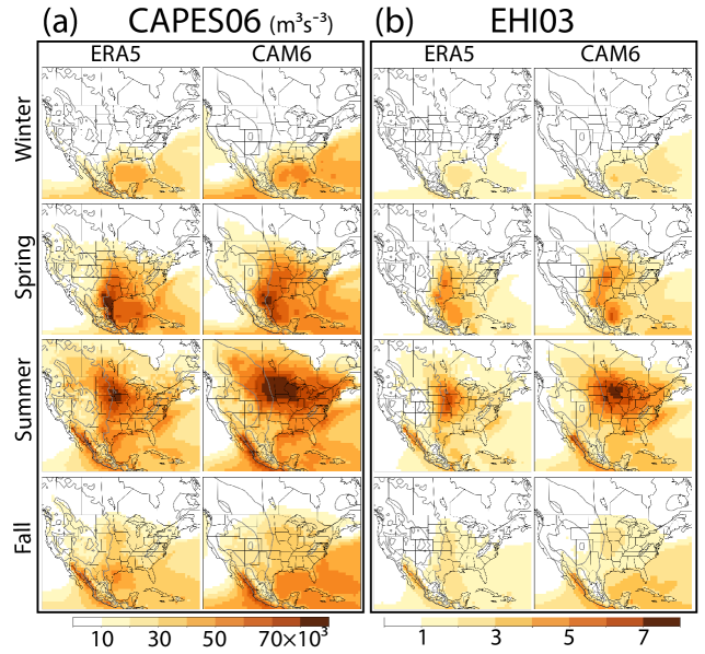
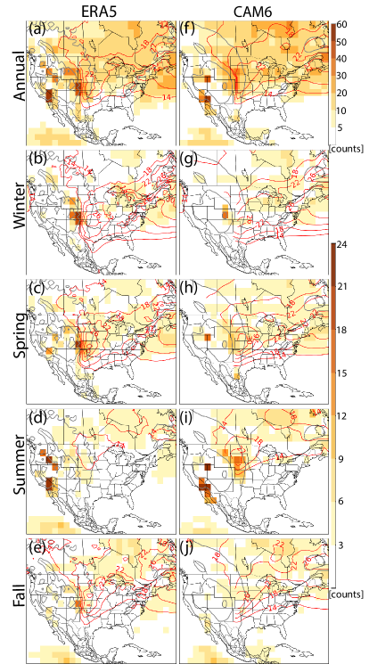
We first analyze the climatology of extreme values (99th percentile) of SLS environmental proxies and parameters over North America in ERA5 and CAM6. The spatial distributions of extreme CAPES06 and EHI03 in ERA5 indicate a similar climatological pattern of such environments (Figure 4a, b). Both extreme CAPES06 and extreme EHI03 achieve a local maximum over southern Texas and over the central United States, consistent with that in the NCEP/NCAR reanalysis (Brooks et al. 2003) and radiosondes (Seeley and Romps 2015). CAM6 simulation broadly reproduces the spatial pattern and amplitude of extreme CAPES06 and EHI03 in ERA5 (Figure 4f, g). However, the local maximum extends farther east covering a larger area of eastern North America, with an enhancement of extreme CAPES06 and EHI03 primarily over the Upper Midwest (Figure 4f, g and S3a, b).
CAM6 biases in extreme CAPES06 are predominantly tied to biases in extreme CAPE rather than S06, as CAM6 overestimates extreme CAPE (Figure 4c, h and S3c) but does an excellent job in reproducing extreme S06 from ERA5 (Figure 4d, i and S3d). Meanwhile, CAM6 biases in extreme EHI03 may be a result of biases in both extreme CAPE and SRH03, as CAM6 overestimates extreme SRH03 as well (Figure 4e, j and S3e). Specifically, CAM6 simulates higher extreme CAPE over much of the eastern half of the United States than ERA5 does (Figure 4c, h and S3c), and higher extreme SRH03 over the central United States and the Midwest (Figure 4e, j and S3e); the simulated extreme S06 is nearly identical to ERA5, which attains its peak in a predominantly zonal band cutting through the central United States associated with the jet stream (Figure 4d, i and S3d). We note that such spatial patterns of the proxies and parameters, as well as biases in CAM6 simulation with respect to ERA5 reanalysis, persist across the high-percentile cases (the 95th, 90th, and 75th percentiles), though the biases decrease moving toward lower percentiles (the 75th percentile; Figure S4).
Though not our focus in this work, convective inhibition (CIN; defined as the negative integral of buoyancy from surface to the level of free convection) is also a key parameter associated with SLS activity and environments, as CIN provides a measure of the lower tropospheric stability that serves as possible barriers to the initiation of conditional instability (Williams and Renno 1993; Chen et al. 2020). CIN extremes distribute broadly similar to CAPES06 and EHI extremes, and are overestimated by CAM6 as well (Figure S5). Deeper analysis for CIN representations in reanalysis datasets or climate models and the associated biases is desirable for future work.
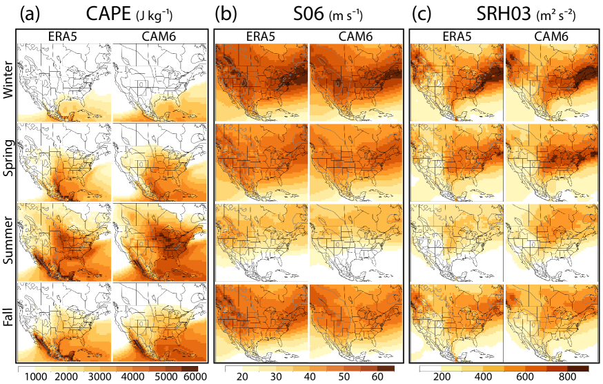
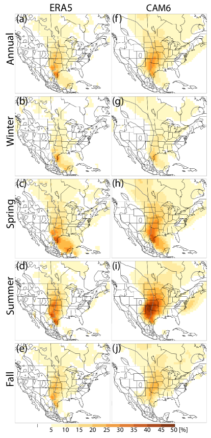
We next analyze the seasonal cycle. Extreme CAPES06 and EHI03 in both ERA5 and CAM6 exhibit a strong seasonal cycle that peaks in warm seasons (spring and summer) (Figure 5), consistent with Tippett et al. (2015). Specifically, the local maximum in spring occurs over southern Texas and shifts to the central United States in summer. A similar seasonal cycle is found in extreme CAPE (Figure 6a), whereas the extreme S06 and SRH03 show an opposite seasonal phase that peaks in winter and reaches a minimum in summer (Figure 6b, c). Biases in these SLS environments from CAM6 also exhibit a significant seasonal variation, as all proxies and parameters are biased higher in summer than in other seasons (Figure S6).
Note that past work has also analyzed the number of days with significant SLS environments () to quantify SLS environments, such as the with CAPES06 10,000 m3 s-3 (Brooks et al. 2003; Trapp et al. 2007, 2009; Diffenbaugh et al. 2013; Seeley and Romps 2015; Hoogewind et al. 2017) or the with CAPES06 20,000 m3 s-3 (Gensini and Ashley 2011; Gensini et al. 2014b; Gensini and Mote 2015). The results of this method can differ from the high-percentile method used here (Singh et al. 2017), as is a pure frequency that does not account for the magnitude above threshold. For comparison, we calculate the climatological and seasonal cycle of with CAPES06 exceeding 10,000 m3 s-3 and 20,000 m3 s-3 respectively in ERA5 reanalysis (Figure S7). Relative to the 99th percentile, the annual with CAPES06 exceeding 10,000 m3 s-3 is shifted toward the southern United States with the local maximum confined to southern Texas (Figure S7a), whereas distributions of the with CAPES06 exceeding 20,000 m3 s-3 are broadly similar to distributions of the 99th percentile of CAPES06 (Figure S7f–j). This is likely because cases with the lower threshold of CAPES06 are weighted more by CAPE than S06, and thus the distribution of is dominated by that of high CAPE which both show small seasonal variations over southern Texas, especially in spring and summer (Figure S7b–e and 7a). The with EHI03 1 is calculated as well, which indicates similar distribution pattern to EHI03 extremes (Figure S7k–o).
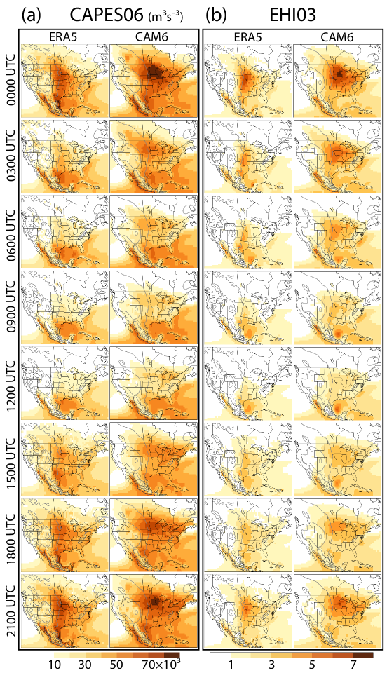
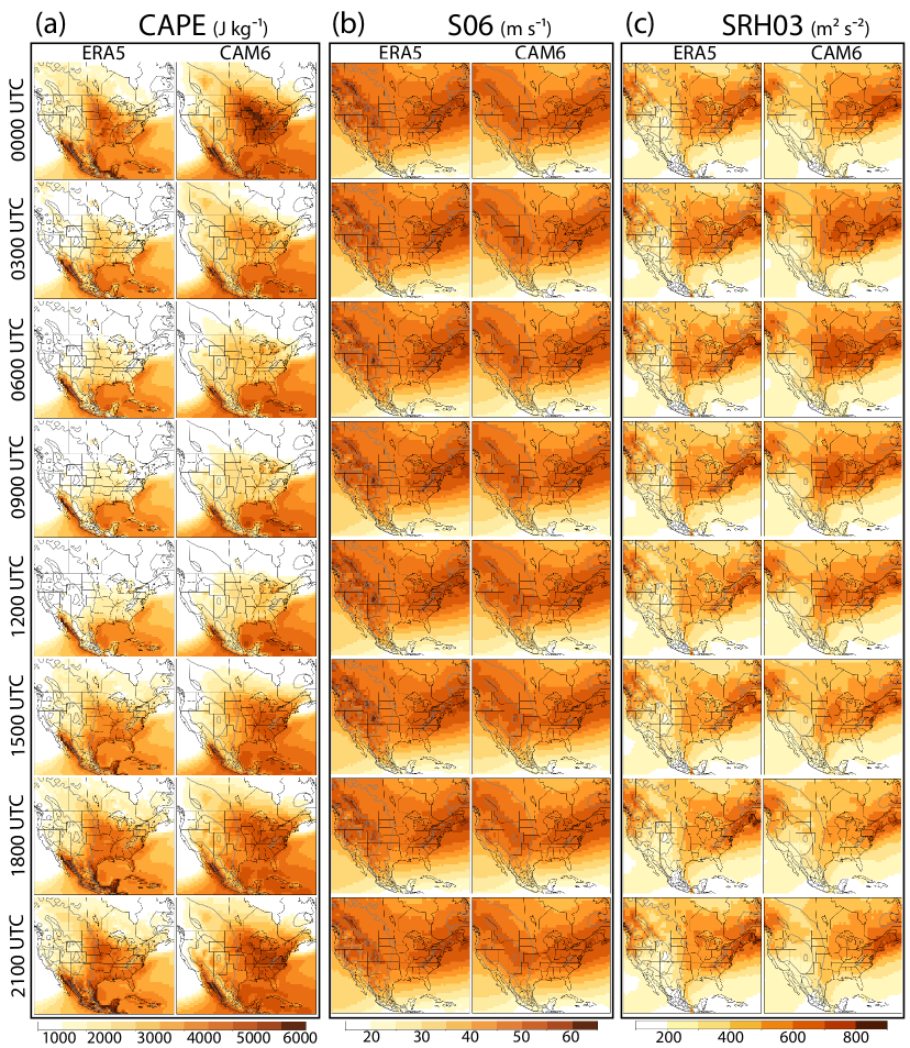
We next analyze the diurnal cycle. Extreme CAPES06 (Figure 7a) and EHI03 (Figure 7b) in both ERA5 and CAM6 exhibit a strong diurnal cycle, particularly in the continental interior where the diurnal cycle peaks during the late afternoon to early evening (2100–0000 UTC) and reaches a minimum in the early morning (0900–1200 UTC). Such diurnal cycle behavior also exists along the Gulf and Atlantic coasts but with a much smaller amplitude, resembling the diurnal variation over ocean. These results are in line with past work on the diurnal variation of deep convection over North America (Wallace 1975; Nesbitt and Zipser 2003; Tian et al. 2005). The diurnal cycle of extreme CAPES06 and EHI03 is dominated by that of extreme CAPE (Figure 8a), whereas the amplitude of the diurnal cycle of extreme S06 (Figure 8b) is relatively small and extreme SRH03 peaks later (at around 0600 UTC) than extreme CAPES06 and EHI03 (Figure 8c). The diurnal cycle signal of extreme SRH03 is strongest over the central United States, associated with the diurnal oscillation of the Great Plains low-level jets. Biases in these SLS environments from CAM6 also exhibit diurnal variations similar to the behaviors of the proxies and parameters themselves (Figure S8).
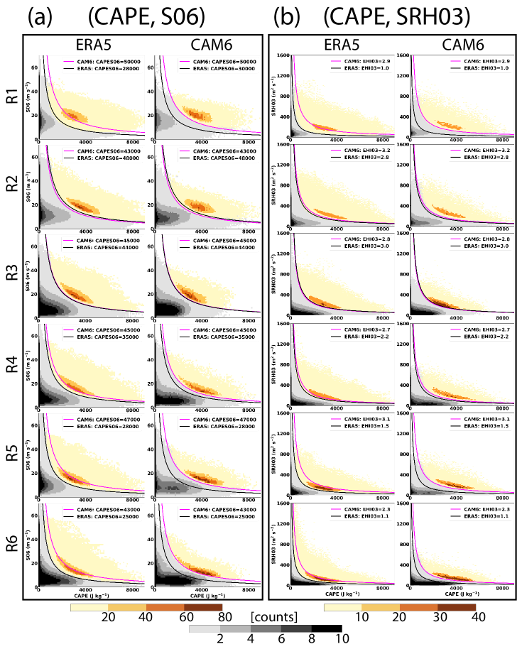
How is extreme CAPES06 or EHI03 affected by its constituent parameters? To more precisely answer this question, we analyze the joint PDF of (CAPE, S06) and (CAPE, SRH03) within each box (R1–R6 in Figure 1b). We analyze the entire joint distribution with special emphasis added to the top 1% cases of CAPES06 and EHI03. Both ERA5 and CAM6 indicate that the CAPES06 and EHI03 extremes consist of large-to-extreme CAPE but moderate-to-small S06 and SRH03 (Figure 9), as was found by Diffenbaugh et al. (2013). Meanwhile, the S06 and SRH03 extremes are associated with small values of CAPE, corresponding to the high-shear, low-CAPE environments (defined as CAPE 500 J kg -1 and S06 18 m s -1) (Guyer and Dean 2010; Sherburn and Parker 2014; Sherburn et al. 2016). These results are also evident in the seasonal cycles described above (Figure 5, 6): high CAPES06 and EHI03 in summer are associated with very high CAPE but relatively low S06 and SRH03, while the high-shear, low-CAPE environments, corresponding to low CAPES06 and EHI03, are concentrated in winter over land. The joint PDFs also indicate that CAPES06 and EHI03 extremes are greater in CAM6 than in ERA5 for regions over the northern Great Plains (R1) and southeastern United States (R5, R6), where the joint PDF shifts toward higher (CAPE, S06) and (CAPE, SRH03). Meanwhile, the difference in the PDFs between ERA5 and CAM6 is relatively small over south-central United States (R2–R4).
4.2 SLS-Relevant Synoptic-Scale Features
4.2.1 Southerly GPLLJ
ERA5 southerly GPLLJ frequency is concentrated primarily over the central and southern Great Plains (Figure 10a), with a seasonal frequency peak (up to 40%) in spring and summer (Figure 10b–e). The local maximum is located in southern Texas in spring and shifts to southwestern Texas and western Oklahoma in summer, consistent with results of NARR reanalysis (Walters et al. 2014; Doubler et al. 2015) and observations (Bonner 1968; Walters et al. 2014). CAM6 broadly reproduces the spatial pattern and amplitude of the southerly GPLLJ frequency (Figure 10f–j), except for summer when the frequency percentage in CAM6 (up to 50% over western Oklahoma; Figure 10i) is much higher than that in ERA5. This increased occurrence of southerly GPLLJ indicates stronger mean low-level winds in CAM6, which contribute to the positive biases in SRH03 over the central United States as well. Meanwhile, more moisture could be transported from the Gulf of Mexico (Helfand and Schubert 1995; Higgins et al. 1997), which may partially explain the enhanced CAPE in CAM6.
4.2.2 Dryline
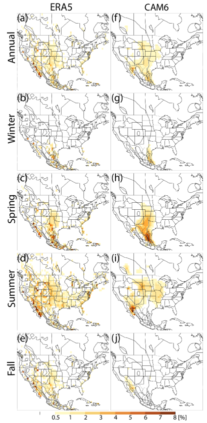
ERA5 dryline frequency is also concentrated in the central and southern Great Plains (Figure 11a), with a seasonal frequency peak (up to 8%) in spring over southwestern Texas (Figure 11c). The distribution shifts poleward into the central plains in summer with a reduced frequency percentage (4%) but spanning a larger area (Figure 11d). These results are qualitatively similar to observations by Schaefer (1974) and Hoch and Markowski (2005), though the amplitude of dryline occurrence is lower than Hoch and Markowski (2005) owing to the stricter criteria used in this work in an effort to distinguish drylines from fronts. CAM6 performs well in reproducing the dryline distribution, as the spatial pattern and amplitude of dryline frequency over the Great Plains and its seasonal variation are broadly similar to that in ERA5 (Figure 11f–j). ERA5 appears to better identify the less-frequent drylines over the far eastern United States (Duell and Van Den Broeke 2016), perhaps owing to its higher horizontal resolution that may permit detection of smaller-scale gradients in surface specific humidity. Meanwhile, ERA5 identifies a number of strong horizontal moisture gradient along the east coast, especially in summer, while these may not correspond with typical drylines over the Great Plains.
4.2.3 EML
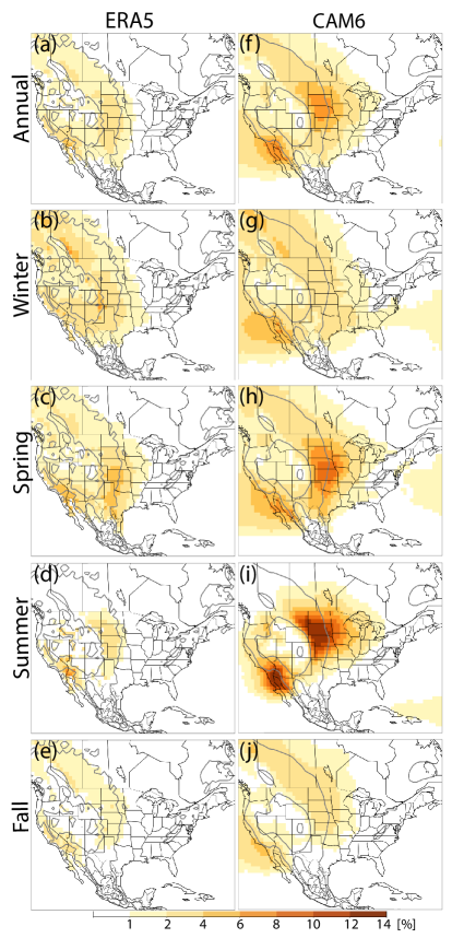
ERA5 EML frequency is again concentrated over the Great Plains (Figure 12a), with a seasonal frequency peak in spring over south-central United States (6%; Figure 12c), consistent with Lanicci and Warner (1991a). The local maximum shifts poleward to South Dakota and Nebraska in summer with a reduced frequency percentage (4%; Figure 12d), qualitatively similar to findings of Ribeiro and Bosart (2018). Note that the amplitude of EML occurrence is sensitive to the identification criteria: the criteria with 7.5 K km-1 for the minimum lapse rate and 150 hPa for the minimum EML depth significantly increase the frequency percentage of EML in ERA5 (e.g., 24% in spring and 20% in summer; not shown). CAM6 successfully reproduces these spatial patterns (Figure 12f–j). However, it exhibits a significant positive bias, particularly in summer (14% over South Dakota), which is associated with the generally larger mid-level lapse rate in CAM6 than in ERA5 (analyzed below in Figure 14). These enhanced EMLs potentially produce more CAPE, which may also partially explain the enhanced CAPE in CAM6.
4.2.4 Extratropical cyclone activity
ERA5 cyclone track frequency has its primary local maximum to the lee of the Rocky Mountains in both the annual mean (Figure 13a) and through the seasonal cycle (Figure 13b–e), which is linked to cyclogenesis on the leeside of the Rocky Mountains. Secondary local maxima are also found over the Great Lakes and off the Northeastern United States coast, in line with findings of Reitan (1974) and Zishka and Smith (1980). Seasonal variation of cyclone tracks is characterized by a decrease in the frequency and a poleward shift of the local maximum from winter and spring (24 counts over southeastern Colorado) to summer (9 counts over Montana-South Dakota), qualitatively similar to past work (Reitan 1974; Zishka and Smith 1980; Eichler and Higgins 2006). Similar results are evident for EKE, as the core of EKE shifts from northwestern Oklahoma in winter to North Dakota in summer. CAM6 broadly reproduces the spatial pattern and amplitude of cyclone tracks and EKE (Figure 13f–j). The cyclone track frequency over southeastern Colorado in CAM6 is smaller than that in ERA5 during winter, spring, and fall, likely due to the coarser horizontal resolutions (Chang et al. 2013). The major difference between CAM6 and ERA5 occurs in summer (Figure 13d, i) when CAM6 produces more cyclone tracks and higher EKE over the central and northern Great Plains than ERA5 (roughly 21 vs. 9 counts and 22 vs. 14 m2 s-2), which may contribute to the positive bias in CAM6 SLS environments in summer relative to ERA5.
Overall, both ERA5 and CAM6 produce qualitatively reasonable climatologies of the key synoptic-scale features over North America. The SLS environments are closely related to these synoptic-scale features as they have consistent climatological behavior in terms of their spatial distributions and seasonal cycles: (1) both SLS environments and the associated synoptic-scale features occur typically in warm seasons (spring or summer) to the east of the Rocky Mountains; and (2) they all exhibit a poleward shift of the local maximum from winter to summer and an equatorward shift again from summer to winter. Compared with ERA5, CAM6 overestimates SLS environments, principally due to a positive bias in extreme CAPE and to a lesser degree SRH03, particularly in summer over much of the eastern half of the United States. These results are consistent with the positive biases in most synoptic-scale features (GPLLJ, EML, and extratropical cyclone activity).
4.3 Biases in the mean-state atmosphere
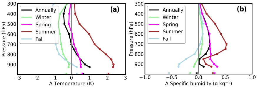
In an effort to better understand these biases in CAM6, we analyze differences in the mean-state atmosphere, which may provide insight into underlying causes (Trapp et al. 2007; Diffenbaugh et al. 2013). Compared to ERA5, the CAM6 summer-mean atmosphere over the eastern half of the United States (100–62∘W, 25–49∘N; Figure 14 and S9) is characterized by higher surface and lower-tropospheric temperatures (+2 K), enhanced low-to-mid-level (900–500-hPa) lapse rates (+0.5 K (100 hPa)-1) that accounts for the overestimated EMLs, and higher specific humidity at the surface (+0.3 g kg-1) and mid-levels (+0.4 g kg-1 averaged through 800–400 hPa). The high biases in summertime extreme CAPE and the combined proxies in CAM6 is attributed primarily to increases in the surface specific humidity. This attribution is supported by high, statistically significant (p0.001) linear pattern correlations () between biases in the extreme CAPE, CAPES06, and EHI03 and biases in the surface specific humidity over the eastern half of the United States ( 0.81, 0.72, and 0.80, respectively); generally small or statistically insignificant pattern correlations () are found with biases in surface temperature, low-to-mid-level lapse rate, or mid-level specific humidity. The summer-mean wind field at the surface and the upper levels in CAM6 and ERA5 is similar, though CAM6 produces slightly stronger upper-level jet streams over northern North America and slightly stronger surface onshore winds over Texas (Figure S9), helping explain the relatively small biases in extreme S06; while the southerly onshore winds over the Great Plains from the Gulf of Mexico are further enhanced in CAM6 at 900–850 hPa (not shown), consistent with the increased southerly GPLLJs and the positive bias of extreme SRH03 over the central Great Plains. Similar features are also evident in Spring though with smaller magnitude. As for winter and fall, the difference between ERA5 and CAM6 in the mean-state atmosphere is relatively small (Figure 14 and S9), consistent with the comparable climatologies of SLS environments and synoptic-scale features analyzed above between ERA5 and CAM6 during these seasons.
These mean low-level warm and moist biases over the eastern half of the United States in CAM6 are associated with systematic warm and dry biases over the central United States while warm and moist biases over the eastern third of the United States (Figure S9a) that have been found to persist in many generations of regional and global climate models (Klein et al. 2006; Cheruy et al. 2014; Mueller and Seneviratne 2014; Lin et al. 2017). Explanation for such systematic bias over the central United States have been proposed, including soil moisture deficit (Koster et al. 2004; Phillips and Klein 2014) or precipitation deficit (Lin et al. 2017) that alters the lower-tropospheric mean state via land-atmosphere feedback processes in climate models (Koster and Suarez 2001; Mo and Juang 2003). How precisely these systematic model biases over the eastern half of the United States affect the SLS environments and synoptic-scale features is a worthy topic left for future work.
4.4 Synoptic Composites for Extreme Cases
Finally, we compare composite patterns of synoptic anomalies associated with extreme SLS environments across our sub-regions over the eastern half of the United States (i.e., R1–R6 defined in Figure 1b) between ERA5 and CAM6. Here, our analysis focuses on R1 and R6. R1 represents the region of the primary local maximum of SLS environments from the ERA5 reanalysis and CAM6 simulation, though the actual SLS occurrence maximum is further south (Agee et al. 2016); R6 is known to exhibit different behavior from the central United States and has shown a positive trend of SLS occurrence in recent decades (Agee et al. 2016; Gensini and Brooks 2018).
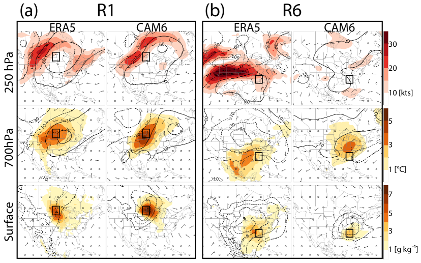
For region R1 over the eastern North Dakota and South Dakota (Figure 15a; ERA5: 166 cases; CAM6: 92 cases), the ERA5 composite yields an enhanced ridge at 250 hPa whose axis extends from northern Texas to North Dakota, with an intensified jet streak along the United States-Canada border (+20–30-kts anomalies). This enhanced upper-level ridge forcing is associated with enhanced southwesterly flow at 700 hPa, which advects more warm and dry air from the elevated terrain eastward toward the Great Plains. Near the surface, the region is located on the southeast side of a trough anomaly extending southward from south-central Canada whose south-southwesterly flow has advected considerable moisture into the region. This composite pattern is similar to that found to be associated with progressive derechos (Johns 1993; Bentley et al. 2000; Guastini and Bosart 2016). CAM6 reproduces this composite pattern, though the 700-hPa warm advection is stronger and the surface trough anomaly is replaced by a slightly more intense cyclonic anomaly centered within the region.
Composite synoptic patterns for cases in the central-southern Great Plains (R2–R4) and over Indiana (R5) are broadly similar between ERA5 and CAM6, and also indicate a similar setup to that in R1, though the relative position of synoptic features varies across regions (Figure S10). In general, a significantly intensified jet streak exists near the region at 250 hPa (except for R5 in CAM6 whose 250-hpa anomalies are relatively small). At 700 hPa, the region is located to the east or northeast of a warm air mass upstream, which supplies substantial warm air into the region due to the enhanced prevailing westerly or southwesterly winds. Near-surface air exhibits a deep trough or cyclonic anomaly with the region located to the east or southeast of the trough axis or the cyclonic center. As a result, robust advection of warm, moist air from the Gulf of Mexico into the region is found in the lower troposphere. These synoptic composites are broadly similar to the classic patterns of severe weather outbreaks over the Great Plains (Barnes and Newton 1986; Johns and Doswell III 1992; Johns 1993; Mercer et al. 2012).
The synoptic composite for sub-region R6 over the southeastern United States (Figure 15b; ERA5: 40 cases; CAM6: 96 cases) differs from the other sub-regions as well as between ERA5 and CAM6. The ERA5 composite yields a much more intense jet stream (anomaly 30 kts) over the central United States at 250 hPa and a subtle shortwave trough at 700 hPa. Near the surface, a strong extratropical cyclone occupies much of the eastern half of North America with a low pressure anomaly centered over the central United States. The region (R6) is located to the southeast of the surface low. One key difference from the other regions is that this area is directly influenced by the flow on the west side of the North Atlantic Subtropical High, which enhances the southwesterly low-level winds and moisture advection over the region (Stahle and Cleaveland 1992; Miller and Mote 2017). The CAM6 composite reproduces this near-surface flow pattern, but at higher levels it yields a broad ridge at 250- and 700-hPa with slight enhancement on the geopotential height and without any anomalous jet streak enhancement to the northwest of the region at 250 hPa. The surface cyclonic anomaly is weaker in CAM6 than in ERA5, causing less moisture transport into the region.
Overall, the common synoptic anomaly patterns associated with extreme SLS environments show small variations across sub-regions over much of the eastern half of the United States (R1–R5), where CAM6 also compares well with ERA5. The southeastern United States (R6) behavior differs somewhat from the other regions, as well as between ERA5 and CAM6, which implies differences in the generation of SLS environments in the Southeast as compared to farther inland. The SLS environments in the Southeast involve a significant portion of high-shear, low-CAPE environments (Guyer and Dean 2010; Sherburn and Parker 2014; Sherburn et al. 2016), which are known to be associated with more difficult forecasting of SLS activity (Miller and Mote 2017). This also implies that the extreme CAPES06 or EHI03 used may be not broadly applicable to identify SLS environments over the Southeast, as they in general capture high-CAPE environments while miss high-shear low-CAPE cases (Figure 9), and thus the composite synoptic patterns for R6 may be less representative of the SLS events in the Southeast. Sufficient low-level moisture supply is clearly essential for significant SLS environments, as all composite analyses reveal robust moisture transport at low levels. Deeper composite analysis using other composite methods such as empirical orthogonal functions (EOFs; Schaefer and Doswell III 1984), rotated principal component analysis (RPCA; Jones et al. 2004; Mercer et al. 2012), or self-organizing maps (SOMs; Sheridan and Lee 2011) would be a valuable path for future work.
5 Conclusions
This work provides a comprehensive climatological analysis and evaluation of SLS environments, and the associated synoptic-scale features that frequently generate them, in the ERA5 reanalysis data and CAM6 climate model simulation. Unlike reanalysis datasets, climate models, including CAM6, do not reproduce the observed daily weather, but they both are able to capture statistical states (e.g., the mean or extremes) for a climate. Thus, we analyzed the overall climatology, as well as seasonal and diurnal cycles, of SLS environments and the occurrence frequency of the synoptic-scale features in the ERA5 reanalysis and a CAM6 AMIP-style simulation for years of 1980–2014 over North America. Here, SLS environments are measured by extreme values (defined as the 99th percentile) of two environmental proxies for SLS favorability, CAPES06 (the product of CAPE and S06) and EHI03 (proportional to the product of CAPE and SRH03), and their constituent parameters (CAPE, S06, and SRH03). Key synoptic-scale features commonly associated with the generation of SLS environments analyzed in this work include southerly Great Plains low-level jets, drylines, elevated mixed layers, and extratropical cyclone activity. Biases in these SLS environments and synoptic-scale features from CAM6 simulation were attributed to biases in the mean-state. Finally, composite analysis was conducted for six sub-regions over the eastern half of the United States to characterize the common synoptic patterns associated with significant SLS environments and assess their CAM6 model representation as compared to ERA5 reanalysis. Primary results are summarized as follows:
-
1.
ERA5 reanalysis reasonably reproduces the observed (radiosonde) spatiotemporal distribution of SLS environments, with relatively low biases and strong correlations particularly over the Great Plains. Kinematic parameters (S06 and SRH03) are in general better estimated by ERA5 reanalysis than thermodynamic parameters (CAPE), especially for stations in the Mountain west and along the east coast where terrain effects are likely large.
-
2.
Climatological patterns of extreme SLS environments over North America are reasonably well-captured by the ERA5 reanalysis and CAM6 simulation. Both ERA5 and CAM6 representations of extreme CAPES06 and EHI03 indicate qualitatively similar annual, seasonal, and diurnal climatologies of extreme SLS environments. Local maxima are found over southern Texas in spring and shift to the central United States in summer. The diurnal cycle peaks during the late afternoon and early evening with a minimum in the early morning, with larger amplitude over the continental interior and smaller amplitude in coastal regions. Extreme values of CAPES06 or EHI03 typically consist of very high CAPE and moderate-to-small S06 or SRH03, and thus the climatological behavior of these proxies are dominated by the behavior of CAPE extremes, not S06 or SRH03 extremes. This implies that extreme CAPES06 and EHI03 is less representative of high-shear, low-CAPE environments which contribute to a considerable portion of SLS environments in the Southeast.
-
3.
Climatologies of key synoptic-scale features over North America are reasonably captured by the ERA5 reanalysis and CAM6 simulation as well. Southerly Great Plains low-level jets, drylines, elevated mixed layers, and extratropical cyclone activity in both ERA5 and CAM6 are most frequent east of the Rocky Mountains in warm seasons. Both ERA5 and CAM6 capture the strong linkage between SLS environments and these synoptic-scale features, as the spatial pattern and seasonal variation of the occurrence frequency of these synoptic-scale features are highly consistent with that of SLS environments.
-
4.
Biases between the CAM6 simulation and ERA5 reanalysis over the eastern United States are largest during summer: (1) CAPE extremes are biased high in CAM6 over much of the eastern half of the United States, which is primarily attributed to the enhanced surface specific humidity in CAM6; (2) SRH03 extremes are biased slightly high, which is primarily attributed to the stronger mean-state low-level winds in CAM6 than ERA5 and more frequent southerly Great Plains low-level jets; (3) elevated mixed layer frequency is biased high, which is primarily attributed to a steeper mean-state mid-level lapse rate and further enhances CAPE; and (4) taken together, the combined proxies CAPES06 and EHI03 are each biased high.
-
5.
The composite synoptic patterns favorable for extreme SLS environments within six sub-regions across the eastern United States in the ERA5 reanalysis indicate an intensified upper-level jet streak in the vicinity of the region, sufficient warm and dry air advection from the elevated terrains eastward toward the Great Plains, and robust low-level moisture transport from the Gulf of Mexico due to the enhanced prevailing southerly or southwesterly winds east of a surface trough or cyclonic anomaly. CAM6 successfully reproduces these structures found in ERA5 for most regions. The principal exception is over the southeastern United States in CAM6 where the influence of the North Atlantic Subtropical High is also important, highlighting differences in climatological forcing that may translate to different behavior and predictability of severe weather itself, as has been identified in past work.
These results suggest that the ERA5 reanalysis data reasonably reproduce SLS environments and synoptic-scale features, and climate models such as CAM6 can be useful tools to investigate climate controls on the generation of SLS environments over North America. Meanwhile, it is necessary to be aware of the biases in climate models (e.g., the systematic biases in surface moisture and temperature over the central and eastern United States), which may affect the interpretation of their projections. To further understand the formation of SLS environments within climate system, future work can use idealized climate modeling experiments to quantitatively test both the detailed linkages between key synoptic-scale features and SLS environments, as well as how climate-scale boundary forcing fundamentally controls the spatiotemporal distribution of SLS environments on Earth.
Acknowledgements.
The authors thank Larry Oolman (University of Wyoming) for providing radiosonde data. The authors thank Editor Dr. Xin-Zhong Liang and three anonymous reviewers for their feedback in improving this manuscript. The authors would like to acknowledge high-performance computing support from Cheyenne (doi:10.5065/D6RX99HX) provided by NCAR’s Computational and Information Systems Laboratory, sponsored by the National Science Foundation, for the simulation and data analysis performed for this work. This research was also supported in part through computational resources provided by Information Technology at Purdue, West Lafayette, Indiana. Li and Chavas were supported by NSF grant 1648681. Reed was supported by the NSF grant AGS1648629, as well as the U.S. Department of Energy Office of Science (DE-SC0019459).References
- Agee et al. (2016) Agee, E., J. Larson, S. Childs, and A. Marmo, 2016: Spatial redistribution of U.S. tornado activity between 1954 and 2013. Journal of Applied Meteorology and Climatology, 55 (8), 1681–1697, https://doi.org/10.1175/JAMC-D-15-0342.1.
- Allen and Karoly (2014) Allen, J. T., and D. J. Karoly, 2014: A climatology of Australian severe thunderstorm environments 1979–2011: inter-annual variability and ENSO influence. International Journal of Climatology, 34 (1), 81–97, https://doi.org/10.1002/joc.3667.
- Banacos and Ekster (2010) Banacos, P. C., and M. L. Ekster, 2010: The association of the elevated mixed layer with significant severe weather events in the northeastern United States. Weather and Forecasting, 25 (4), 1082–1102, https://doi.org/10.1175/2010WAF2222363.1.
- Barnes and Newton (1986) Barnes, S., and C. Newton, 1986: Thunderstorms in the synoptic setting. Thunderstorm Morphology and Dynamics, E, Kessler, Ed., University of Oklahoma Press, 75–111.
- Bentley et al. (2000) Bentley, M. L., T. L. Mote, and S. F. Byrd, 2000: A synoptic climatology of derecho producing mesoscale convective systems in the North-Central Plains. International Journal of Climatology: A Journal of the Royal Meteorological Society, 20 (11), 1329–1349, https://doi.org/10.1002/1097-0088(200009)20:11¡1329::AID-JOC537¿3.0.CO;2-F.
- Blackmon (1976) Blackmon, M. L., 1976: A climatological spectral study of the 500 mb geopotential height of the Northern Hemisphere. Journal of the Atmospheric Sciences, 33 (8), 1607–1623, https://doi.org/10.1175/1520-0469(1976)033¡1607:ACSSOT¿2.0.CO;2.
- Blumberg et al. (2017) Blumberg, W. G., K. T. Halbert, T. A. Supinie, P. T. Marsh, R. L. Thompson, and J. A. Hart, 2017: Sharppy: An open-source sounding analysis toolkit for the atmospheric sciences. Bulletin of the American Meteorological Society, 98 (8), 1625–1636, https://doi.org/10.1175/BAMS-D-15-00309.1.
- Bogenschutz et al. (2013) Bogenschutz, P. A., A. Gettelman, H. Morrison, V. E. Larson, C. Craig, and D. P. Schanen, 2013: Higher-order turbulence closure and its impact on climate simulations in the Community Atmosphere Model. Journal of Climate, 26 (23), 9655–9676, https://doi.org/10.1175/JCLI-D-13-00075.1.
- Bonner (1968) Bonner, W. D., 1968: Climatology of the low level jet. Monthly Weather Review, 96 (12), 833–850, https://doi.org/10.1175/1520-0493(1968)096¡0833:COTLLJ¿2.0.CO;2.
- Brooks et al. (2003) Brooks, H. E., J. W. Lee, and J. P. Craven, 2003: The spatial distribution of severe thunderstorm and tornado environments from global reanalysis data. Atmospheric Research, 67, 79–94, https://doi.org/10.1016/S0169-8095(03)00045-0.
- Bunkers et al. (2000) Bunkers, M. J., B. A. Klimowski, J. W. Zeitler, R. L. Thompson, and M. L. Weisman, 2000: Predicting supercell motion using a new hodograph technique. Weather and forecasting, 15 (1), 61–79, https://doi.org/10.1175/1520-0434(2000)015¡0061:PSMUAN¿2.0.CO;2.
- Carlson et al. (1983) Carlson, T. N., S. G. Benjamin, G. S. Forbes, and Y. F. Li, 1983: Elevated mixed layers in the regional severe storm environment: Conceptual model and case studies. Monthly Weather Review, 111 (7), 1453–1474, https://doi.org/10.1175/1520-0493(1983)111¡1453:EMLITR¿2.0.CO;2.
- Chang et al. (2013) Chang, E. K., Y. Guo, X. Xia, and M. Zheng, 2013: Storm-track activity in IPCC AR4/CMIP3 model simulations. Journal of Climate, 26 (1), 246–260, https://doi.org/10.1175/JCLI-D-11-00707.1.
- Chen et al. (2020) Chen, J., A. Dai, Y. Zhang, and K. L. Rasmussen, 2020: Changes in Convective Available Potential Energy and Convective Inhibition under global warming. Journal of Climate, 33 (6), 2025–2050, https://doi.org/10.1175/JCLI-D-19-0461.1.
- Cheruy et al. (2014) Cheruy, F., J. Dufresne, F. Hourdin, and A. Ducharne, 2014: Role of clouds and land-atmosphere coupling in midlatitude continental summer warm biases and climate change amplification in CMIP5 simulations. Geophysical Research Letters, 41 (18), 6493–6500, https://doi.org/10.1002/2014GL061145.
- Cordeira et al. (2017) Cordeira, J. M., N. D. Metz, M. E. Howarth, and T. J. G. Jr, 2017: Multiscale upstream and in situ precursors to the elevated mixed layer and high-impact weather over the Midwest United States. Weather and Forecasting, 32 (3), 905–923, https://doi.org/10.1175/WAF-D-16-0122.1.
- Davies-Jones (1993) Davies-Jones, R. P., 1993: Helicity trends in tornado outbreaks. 17th Conf. on Severe Local Storms, St. Louis, MO, Amer. Meteor. Soc., 56–60.
- Davies-Jones (2002) Davies-Jones, R. P., 2002: Linear and nonlinear propagation of supercell storms. Journal of the Atmospheric Sciences, 59 (22), 3178–3205, 10.1175/1520-0469(2003)059¡3178:LANPOS¿2.0.CO;2.
- Davies-Jones (2003) Davies-Jones, R. P., 2003: Reply. Journal of the Atmospheric Sciences, 60 (19), 2420–2426, https://doi.org/10.1175/1520-0469(2003)060¡2420:R¿2.0.CO;2.
- Davies-Jones et al. (1990) Davies-Jones, R. P., D. Burgess, and M. Foster, 1990: Test of helicity as a tornado forecast parameter. 16th Conf. on Severe Local Storms, Kananaskis Park, AB, Canada, Amer. Meteor. Soc., 588–592.
- Dee et al. (2011) Dee, D. P., and Coauthors, 2011: The ERA-Interim reanalysis: Configuration and performance of the data assimilation system. Quarterly Journal of the royal meteorological society, 137 (656), 553–597, https://doi.org/10.1002/qj.828.
- Diffenbaugh et al. (2013) Diffenbaugh, N. S., M. Scherer, and R. J. Trapp, 2013: Robust increases in severe thunderstorm environments in response to greenhouse forcing. Proceedings of the National Academy of Sciences, 110 (41), 16 361–16 366, https://doi.org/10.1073/pnas.1307758110.
- Doswell III and Schultz (2006) Doswell III, C., and D. M. Schultz, 2006: On the use of indices and parameters in forecasting severe storms. Electronic Journal of Severe Storms Meteorology, 1 (3), 1–22, https://doi.org/10.1128/AAC.00548-11.
- Doswell III and Bosart (2001) Doswell III, C. A., and L. F. Bosart, 2001: Extratropical synoptic-scale processes and severe convection. American Meteorological Society, https://doi.org/10.1007/978-1-935704-06-5_2.
- Doswell III and Burgess (1993) Doswell III, C. A., and D. W. Burgess, 1993: Tornadoes and Tornadic Storms: A Review of Conceptual Models, 161–172. American Geophysical Union (AGU), 10.1029/GM079p0161.
- Doswell III and Rasmussen (1994) Doswell III, C. A., and E. N. Rasmussen, 1994: The effect of neglecting the virtual temperature correction on CAPE calculations. Weather and forecasting, 9 (4), 625–629, https://doi.org/10.1175/1520-0434(1994)009¡0625:TEONTV¿2.0.CO;2.
- Doubler et al. (2015) Doubler, D. L., J. A. Winkler, X. Bian, C. K. Walters, and S. Zhong, 2015: An NARR-derived climatology of southerly and northerly low-level jets over North America and coastal environs. Journal of Applied Meteorology and Climatology, 54 (7), 1596–1619, https://doi.org/10.1175/JAMC-D-14-0311.1.
- Duell and Van Den Broeke (2016) Duell, R. S., and M. S. Van Den Broeke, 2016: Climatology, synoptic conditions, and misanalyses of Mississippi River Valley drylines. Monthly Weather Review, 144 (3), 927–943, https://doi.org/10.1175/mwr-d-15-0108.1.
- ECMWF (2019) ECMWF, 2019: ERA5 Reanalysis (0.25 Degree Latitude-Longitude Grid). Research Data Archive at the National Center for Atmospheric Research, Computational and Information Systems Laboratory, Boulder CO, URL https://doi.org/10.5065/BH6N-5N20.
- Eichler and Higgins (2006) Eichler, T., and W. Higgins, 2006: Climatology and ENSO-related variability of North American extratropical cyclone activity. Journal of Climate, 19 (10), 2076–2093, https://doi.org/10.1175/JCLI3725.1.
- Eyring et al. (2016) Eyring, V., S. Bony, G. A. Meehl, C. A. Senior, B. Stevens, R. J. Stouffer, and K. E. Taylor, 2016: Overview of the Coupled Model Intercomparison Project Phase 6 (CMIP6) experimental design and organization. Geoscientific Model Development, 9, 1937–1958, https://doi.org/10.5194/gmd-9-1937-2016.
- Farrell and Carlson (1989) Farrell, R. J., and T. N. Carlson, 1989: Evidence for the role of the lid and underunning in an outbreak of tornadic thunderstorms. Monthly Weather Review, 117 (4), 857–871, https://doi.org/10.1175/1520-0493(1989)117¡0857:EFTROT¿2.0.CO;2.
- Fujita (1958) Fujita, T., 1958: Structure and movement of a dry front. Bulletin of the American Meteorological Society, 39 (11), 574–582, https://doi.org/10.1175/1520-0477-39.11.574.
- Gates et al. (1999) Gates, W. L., and Coauthors, 1999: An overview of the results of the Atmospheric Model Intercomparison Project (AMIP I). Bulletin of the American Meteorological Society, 80, 29–55, https://doi.org/10.1175/1520-0477(1999)080¡0029:AOOTRO¿2.0.CO;2.
- Gensini and Ashley (2011) Gensini, V. A., and W. S. Ashley, 2011: Climatology of potentially severe convective environments from the North American Regional Reanalysis. E-Journal of Severe Storms Meteorology, 6 (8), 1–40.
- Gensini and Bravo de Guenni (2019) Gensini, V. A., and L. Bravo de Guenni, 2019: Environmental covariate representation of seasonal US tornado frequency. Journal of Applied Meteorology and Climatology, 58 (6), 1353–1367, https://doi.org/10.1175/JAMC-D-18-0305.1.
- Gensini and Brooks (2018) Gensini, V. A., and H. E. Brooks, 2018: Spatial trends in United States tornado frequency. npj Climate and Atmospheric Science, 1 (1), 1–5, https://doi.org/10.1038/s41612-018-0048-2.
- Gensini and Mote (2014) Gensini, V. A., and T. L. Mote, 2014: Estimations of hazardous convective weather in the United States using dynamical downscaling. Journal of Climate, 27 (17), 6581–6589, https://doi.org/10.1175/JCLI-D-13-00777.1.
- Gensini and Mote (2015) Gensini, V. A., and T. L. Mote, 2015: Downscaled estimates of late 21st century severe weather from CCSM3. Climatic Change, 129 (1–2), 307–321, https://doi.org/10.1007/s10584-014-1320-z.
- Gensini et al. (2014a) Gensini, V. A., T. L. Mote, and H. E. Brooks, 2014a: Severe-thunderstorm reanalysis environments and collocated radiosonde observations. Journal of Applied Meteorology and Climatology, 53 (3), 742–751, https://doi.org/10.1175/JAMC-D-13-0263.1.
- Gensini et al. (2014b) Gensini, V. A., C. Ramseyer, and T. L. Mote, 2014b: Future convective environments using NARCCAP. International Journal of Climatology, 34 (5), 1699–1705, https://doi.org/10.1002/joc.3769.
- Gettelman and Morrison (2015) Gettelman, A., and H. Morrison, 2015: Advanced two-moment bulk microphysics for global models. Part I: Off-line tests and comparison with other schemes. Journal of Climate, 28 (3), 1268–1287, https://doi.org/10.1175/JCLI-D-14-00102.1.
- Golaz et al. (2002) Golaz, J.-C., V. E. Larson, and W. R. Cotton, 2002: A PDF-based model for boundary layer clouds. Part I: Method and model description. Journal of the atmospheric sciences, 59 (24), 3540–3551, https://doi.org/10.1175/1520-0469(2002)059¡3540:APBMFB¿2.0.CO;2.
- Grams et al. (2012) Grams, J. S., R. L. Thompson, D. V. Snively, J. A. Prentice, G. M. Hodges, and L. J. Reames, 2012: A climatology and comparison of parameters for significant tornado events in the United States. Weather and Forecasting, 27 (1), 106–123, https://doi.org/10.1175/waf-d-11-00008.1.
- Guastini and Bosart (2016) Guastini, C. T., and L. F. Bosart, 2016: Analysis of a progressive derecho climatology and associated formation environments. Monthly Weather Review, 144 (4), 1363–1382, https://doi.org/10.1175/MWR-D-15-0256.1.
- Guyer and Dean (2010) Guyer, J. L., and A. R. Dean, 2010: Tornadoes within weak cape environments across the continental United States. 25th Conf. on Severe Local Storms, Denver, CO, Amer. Meteor. Soc.
- Hamill et al. (2005) Hamill, T. M., R. S. Schneider, H. E. Brooks, G. S. Forbes, H. B. Bluestein, M. Steinberg, D. Meléndez, and R. M. Dole, 2005: The May 2003 extended tornado outbreak. Bulletin of the American Meteorological Society, 86 (4), 531–542, https://doi.org/10.1175/bams-86-4-531.
- Hart and Korotky (1991) Hart, J. A., and W. Korotky, 1991: The SHARP workstation v1.50 users guide. National Weather Service, NOAA, US. Dept. of Commerce, 30pp pp., [Available from NWS Eastern Region Headquarters,630 Johnson Ave., Bohemia, NY 11716.].
- Harvey et al. (2014) Harvey, B. J., L. C. Shaffrey, and T. J. Woollings, 2014: Equator-to-pole temperature differences and the extra-tropical storm track responses of the CMIP5 climate models. Climate Dynamics, 43 (5-6), 1171–1182, https://doi.org/10.1007/s00382-013-1883-9.
- Helfand and Schubert (1995) Helfand, H. M., and S. D. Schubert, 1995: Climatology of the simulated Great Plains low-level jet and its contribution to the continental moisture budget of the United States. Journal of Climate, 8 (4), 784–806, https://doi.org/10.1175/1520-0442(1995)008¡0784:COTSGP¿2.0.CO;2.
- Hersbach and Dee (2016) Hersbach, H., and D. Dee, 2016: ERA5 reanalysis is in production. ECMWF newsletter, 147 (7), 5–6.
- Higgins et al. (1997) Higgins, R. W., Y. Yao, E. S. Yarosh, J. E. Janowiak, and K. C. Mo, 1997: Influence of the Great Plains low-level jet on summertime precipitation and moisture transport over the central United States. Journal of Climate, 10 (3), 481–507, https://doi.org/10.1175/1520-0442(1997)010¡0481:IOTGPL¿2.0.CO;2.
- Hoch and Markowski (2005) Hoch, J., and P. Markowski, 2005: A climatology of springtime dryline position in the U.S. Great Plains region. Journal of Climate, 18 (12), 2132–2137, https://doi.org/10.1175/JCLI3392.1.
- Holton (1973) Holton, J. R., 1973: An introduction to dynamic meteorology. American Journal of Physics, 41 (5), 752–754.
- Hoogewind et al. (2017) Hoogewind, K. A., M. E. Baldwin, and R. J. Trapp, 2017: The impact of climate change on hazardous convective weather in the United States: insight from high-resolution dynamical downscaling. Journal of Climate, 30 (24), 10 081–10 100, https://doi.org/10.1175/JCLI-D-16-0885.1.
- Hunter (2007) Hunter, J. D., 2007: Matplotlib: A 2d graphics environment. Computing in Science & Engineering, 9 (3), 90–95, 10.1109/MCSE.2007.55.
- Johns (1993) Johns, R. H., 1993: Meteorological conditions associated with bow echo development in convective storms. Weather and Forecasting, 8 (2), 294–299, https://doi.org/10.1175/1520-0434(1993)008¡0294:MCAWBE¿2.0.CO;2.
- Johns and Doswell III (1992) Johns, R. H., and C. A. Doswell III, 1992: Severe local storms forecasting. Weather and Forecasting, 7 (4), 588–612, https://doi.org/10.1175/1520-0434(1992)007¡0588:SLSF¿2.0.CO;2.
- Jones et al. (2004) Jones, T. A., K. M. McGrath, and J. T. Snow, 2004: Association between NSSL mesocyclone detection algorithm-detected vortices and tornadoes. Weather and forecasting, 19 (5), 872–890, https://doi.org/10.1175/1520-0434(2004)019¡0872:ABNMDA¿2.0.CO;2.
- Kaspi and Schneider (2013) Kaspi, Y., and T. Schneider, 2013: The role of stationary eddies in shaping midlatitude storm tracks. Journal of the Atmospheric Sciences, 70 (8), 2596–2613, https://doi.org/10.1175/jas-d-12-082.1.
- Klein et al. (2006) Klein, S. A., X. Jiang, J. Boyle, S. Malyshev, and S. Xie, 2006: Diagnosis of the summertime warm and dry bias over the US Southern Great Plains in the GFDL climate model using a weather forecasting approach. Geophysical research letters, 33 (18), https://doi.org/10.1029/2006GL027567.
- Koster and Suarez (2001) Koster, R. D., and M. J. Suarez, 2001: Soil moisture memory in climate models. Journal of hydrometeorology, 2 (6), 558–570, https://doi.org/10.1175/1525-7541(2001)002¡0558:SMMICM¿2.0.CO;2.
- Koster et al. (2004) Koster, R. D., and Coauthors, 2004: Regions of strong coupling between soil moisture and precipitation. Science, 305 (5687), 1138–1140, 10.1126/science.1100217.
- Lanicci and Warner (1991a) Lanicci, J. M., and T. T. Warner, 1991a: A synoptic climatology of the elevated mixed-layer inversion over the southern Great Plains in spring. Part I: Structure, dynamics, and seasonal evolution. Weather and Forecasting, 6 (2), 181–197, https://doi.org/10.1175/1520-0434(1991)006¡0181:ASCOTE¿2.0.CO;2.
- Lanicci and Warner (1991b) Lanicci, J. M., and T. T. Warner, 1991b: A synoptic climatology of the elevated mixed-layer inversion over the southern Great Plains in spring. Part II: The life cycle of the lid. Weather and Forecasting, 6 (2), 198–213, https://doi.org/10.1175/1520-0434(1991)006¡0198:ASCOTE¿2.0.CO;2.
- Lanicci and Warner (1991c) Lanicci, J. M., and T. T. Warner, 1991c: A synoptic climatology of the elevated mixed-layer inversion over the southern Great Plains in spring. Part III: Relationship to severe-storms climatology. Weather and Forecasting, 6 (2), 214–226, https://doi.org/10.1175/1520-0434(1991)006¡0214:ASCOTE¿2.0.CO;2.
- Lin et al. (2017) Lin, Y., W. Dong, M. Zhang, Y. Xie, W. Xue, J. Huang, and Y. Luo, 2017: Causes of model dry and warm bias over central US and impact on climate projections. Nature communications, 8 (1), 1–8, https://doi.org/10.1038/s41467-017-01040-2.
- Ludlam (1963) Ludlam, F., 1963: Severe local storms: A review. Severe Local Storms. Meteorological Monographs, vol 5., American Meteorological Society, Boston, MA, 1–32, https://doi.org/10.1007/978-1-940033-56-3_1.
- Mercer et al. (2012) Mercer, A. E., M. B. Richman, C. A. Doswell III, C. M. Shafer, and L. M. Leslie, 2012: Synoptic composites of tornadic and nontornadic outbreaks. Monthly Weather Review, 140 (8), 2590–2608, https://doi.org/10.1175/mwr-d-12-00029.1.
- Miller and Mote (2017) Miller, P. W., and T. L. Mote, 2017: A climatology of weakly forced and pulse thunderstorms in the southeast United States. Journal of Applied Meteorology and Climatology, 56 (11), 3017–3033, https://doi.org/10.1175/JAMC-D-17-0005.1.
- Mo and Juang (2003) Mo, K. C., and H.-M. H. Juang, 2003: Relationships between soil moisture and summer precipitation over the great plains and the southwest. Journal of Geophysical Research: Atmospheres, 108 (D16), https://doi.org/10.1029/2002JD002952.
- Mueller and Seneviratne (2014) Mueller, B., and S. I. Seneviratne, 2014: Systematic land climate and evapotranspiration biases in CMIP5 simulations. Geophysical research letters, 41 (1), 128–134, https://doi.org/10.1002/2013GL058055.
- Neale et al. (2012) Neale, R. B., and Coauthors, 2012: Description of the ncar community atmosphere model: Cam5.0. Technical Report NCAR/TN-486+STR;National Center for Atmospheric Research; Boulder, Colorado, USA, 268pp.
- Nesbitt and Zipser (2003) Nesbitt, S. W., and E. J. Zipser, 2003: The diurnal cycle of rainfall and convective intensity according to three years of TRMM measurements. Journal of Climate, 16 (10), 1456–1475, https://doi.org/10.1175/1520-0442(2003)016¡1456:TDCORA¿2.0.CO;2.
- Parker (2016) Parker, W. S., 2016: Reanalyses and observations: What’s the difference? Bulletin of the American Meteorological Society, 97 (9), 1565–1572, https://doi.org/10.1175/BAMS-D-14-00226.1.
- Phillips and Klein (2014) Phillips, T. J., and S. A. Klein, 2014: Land-atmosphere coupling manifested in warm-season observations on the us southern great plains. Journal of Geophysical Research: Atmospheres, 119 (2), 509–528, https://doi.org/10.1002/2013JD020492.
- Rasmussen (2003) Rasmussen, E. N., 2003: Refined supercell and tornado forecast parameters. Weather and Forecasting, 18 (3), 530–535, https://doi.org/10.1175/1520-0434(2003)18¡530:RSATFP¿2.0.CO;2.
- Rasmussen and Blanchard (1998) Rasmussen, E. N., and D. O. Blanchard, 1998: A baseline climatology of sounding-derived supercell and tornado forecast parameters. Weather and Forecasting, 13 (4), 1148–1164, https://doi.org/10.1175/1520-0434(1998)013¡1148:abcosd¿2.0.co;2.
- Reitan (1974) Reitan, C. H., 1974: Frequencies of cyclones and cyclogenesis for North America, 1951–1970. Monthly Weather Review, 102 (12), 861–868, https://doi.org/10.1175/1520-0493(1974)102¡0861:FOCACF¿2.0.CO;2.
- Rhea (1966) Rhea, J. O., 1966: A study of thunderstorm formation along dry lines. Journal of Applied Meteorology, 5 (1), 58–63, https://doi.org/10.1175/1520-0450(1966)005¡0058:asotfa¿2.0.co;2.
- Ribeiro and Bosart (2018) Ribeiro, B. Z., and L. F. Bosart, 2018: Elevated mixed layers and associated severe thunderstorm environments in South and North Americas. Monthly Weather Review, 146 (1), 3–28, https://doi.org/10.1175/MWR-D-17-0121.1.
- Rieck et al. (2015) Rieck, J. K., C. W. Böning, R. J. Greatbatch, and M. Scheinert, 2015: Seasonal variability of eddy kinetic energy in a global high-resolution ocean model. Geophysical Research Letters, 42 (21), 9379–9386, https://doi.org/10.1002/2015GL066152.
- Robinson et al. (2013) Robinson, E. D., R. J. Trapp, and M. E. Baldwin, 2013: The geospatial and temporal distributions of severe thunderstorms from high-resolution dynamical downscaling. Journal of applied meteorology and climatology, 52 (9), 2147–2161, https://doi.org/10.1175/JAMC-D-12-0131.1.
- Romps et al. (2014) Romps, D. M., J. T. Seeley, D. Vollaro, and J. Molinari, 2014: Projected increase in lightning strikes in the United States due to global warming. Science, 346 (6211), 851–854, https://doi.org/10.1126/science.1259100.
- Rotunno and Klemp (1985) Rotunno, R., and J. Klemp, 1985: On the rotation and propagation of simulated supercell thunderstorms. Journal of the Atmospheric Sciences, 42 (3), 271–292, https://doi.org/10.1175/1520-0469(1985)042¡0271:OTRAPO¿2.0.CO;2.
- Rotunno and Klemp (1982) Rotunno, R., and J. B. Klemp, 1982: The influence of the shear-induced pressure gradient on thunderstorm motion. Monthly Weather Review, 110 (2), 136–151, https://doi.org/10.1175/1520-0493(1982)110¡0136:TIOTSI¿2.0.CO;2.
- Rotunno and Weisman (2003) Rotunno, R., and M. L. Weisman, 2003: Comment on “Linear and nonlinear propagation of supercell storms”. Journal of the Atmospheric Sciences, 60 (19), 2413–2419, https://doi.org/10.1175/1520-0469(2003)060¡2413:COLANP¿2.0.CO;2.
- Russell (2006) Russell, D. R., 2006: Development of a time-domain, variable-period surface-wave magnitude measurement procedure for application at regional and teleseismic distances, Part I: Theory. Bulletin of the Seismological Society of America, 96 (2), 665–677, https://doi.org/10.1785/0120050055.
- Schaefer (1974) Schaefer, J. T., 1974: The life cycle of the dryline. Journal of Applied Meteorology, 13 (4), 444–449, https://doi.org/10.1175/1520-0450(1974)013¡0444:tlcotd¿2.0.co;2.
- Schaefer and Doswell III (1984) Schaefer, J. T., and C. A. Doswell III, 1984: Empirical orthogonal function expansion applied to progressive tornado outbreaks. Journal of the Meteorological Society of Japan. Ser. II, 62 (6), 929–936, https://doi.org/10.2151/jmsj1965.62.6_929.
- Schemm and Schneider (2018) Schemm, S., and T. Schneider, 2018: Eddy lifetime, number, and diffusivity and the suppression of eddy kinetic energy in midwinter. Journal of Climate, 31 (14), 5649–5665, https://doi.org/10.1175/JCLI-D-17-0644.1.
- Schultz et al. (2007) Schultz, D. M., C. C. Weiss, and P. M. Hoffman, 2007: The synoptic regulation of dryline intensity. Monthly Weather Review, 135 (5), 1699–1709, https://doi.org/10.1175/mwr3376.1.
- Seeley and Romps (2015) Seeley, J. T., and D. M. Romps, 2015: The effect of global warming on severe thunderstorms in the United States. Journal of Climate, 28 (6), 2443–2458, https://doi.org/10.1175/JCLI-D-14-00382.1.
- Sherburn and Parker (2014) Sherburn, K. D., and M. D. Parker, 2014: Climatology and ingredients of significant severe convection in high-shear, low-CAPE environments. Weather and forecasting, 29 (4), 854–877, https://doi.org/10.1175/WAF-D-13-00041.1.
- Sherburn et al. (2016) Sherburn, K. D., M. D. Parker, J. R. King, and G. M. Lackmann, 2016: Composite environments of severe and nonsevere high-shear, low-CAPE convective events. Weather and Forecasting, 31 (6), 1899–1927, https://doi.org/10.1175/waf-d-16-0086.1.
- Sheridan and Lee (2011) Sheridan, S. C., and C. C. Lee, 2011: The self-organizing map in synoptic climatological research. Progress in Physical Geography, 35 (1), 109–119, https://doi.org/10.1177/0309133310397582.
- Singh et al. (2017) Singh, M. S., Z. Kuang, E. D. Maloney, W. M. Hannah, and B. O. Wolding, 2017: Increasing potential for intense tropical and subtropical thunderstorms under global warming. Proceedings of the National Academy of Sciences, 114 (44), 11 657–11 662, https://doi.org/10.1073/pnas.1707603114.
- Stahle and Cleaveland (1992) Stahle, D. W., and M. K. Cleaveland, 1992: Reconstruction and analysis of spring rainfall over the southeastern U.S. for the past 1000 years. Bulletin of the American Meteorological Society, 73 (12), 1947–1961, https://doi.org/10.1175/1520-0477(1992)073¡1947:raaosr¿2.0.co;2.
- Tamarin and Kaspi (2016) Tamarin, T., and Y. Kaspi, 2016: The poleward motion of extratropical cyclones from a potential vorticity tendency analysis. Journal of the Atmospheric Sciences, 73 (4), 1687–1707, https://doi.org/10.1175/jas-d-15-0168.1.
- Tang et al. (2019) Tang, B. H., V. A. Gensini, and C. R. Homeyer, 2019: Trends in United States large hail environments and observations. npj Climate and Atmospheric Science, 2 (1), 1–7, https://doi.org/10.1038/s41612-019-0103-7.
- Taszarek et al. (2018) Taszarek, M., H. E. Brooks, B. Czernecki, P. Szuster, and K. Fortuniak, 2018: Climatological aspects of convective parameters over Europe: a comparison of ERA-Interim and sounding data. Journal of Climate, 31 (11), 4281–4308, https://doi.org/10.1175/JCLI-D-17-0596.1.
- Thompson et al. (2003) Thompson, R. L., R. Edwards, J. A. Hart, K. L. Elmore, and P. Markowski, 2003: Close proximity soundings within supercell environments obtained from the rapid update cycle. Weather and Forecasting, 18 (6), 1243–1261, https://doi.org/10.1175/1520-0434(2003)018¡1243:CPSWSE¿2.0.CO;2.
- Tian et al. (2005) Tian, B., I. M. Held, N. C. Lau, and B. J. Soden, 2005: Diurnal cycle of summertime deep convection over North America: A satellite perspective. Journal of Geophysical Research D: Atmospheres, 110 (8), 1–10, https://doi.org/10.1029/2004JD005275.
- Tippett et al. (2015) Tippett, M. K., J. T. Allen, V. A. Gensini, and H. E. Brooks, 2015: Climate and hazardous convective weather. Current Climate Change Reports, 1 (2), 60–73, https://doi.org/10.1007/s40641-015-0006-6.
- Tippett et al. (2016) Tippett, M. K., C. Lepore, and J. E. Cohen, 2016: More tornadoes in the most extreme US tornado outbreaks. Science, 354 (6318), 1419–1423, https://doi.org/10.1126/science.aah7393.
- Tochimoto and Niino (2015) Tochimoto, E., and H. Niino, 2015: Structural and environmental characteristics of extratropical cyclones that cause tornado outbreaks in the warm sector: A composite study. Monthly Weather Review, 144 (3), 945–969, https://doi.org/10.1175/mwr-d-15-0015.1.
- Trapp et al. (2007) Trapp, R. J., N. S. Diffenbaugh, H. E. Brooks, M. E. Baldwin, E. D. Robinson, and J. S. Pal, 2007: Changes in severe thunderstorm environment frequency during the 21st century caused by anthropogenically enhanced global radiative forcing. Proceedings of the National Academy of Sciences, 104 (50), 19 719–19 723, https://doi.org/10.1073/pnas.0705494104.
- Trapp et al. (2009) Trapp, R. J., N. S. Diffenbaugh, and A. Gluhovsky, 2009: Transient response of severe thunderstorm forcing to elevated greenhouse gas concentrations. Proceedings of the National Academy of Sciences, 36 (1), https://doi.org/10.1029/2008GL036203.
- Trapp et al. (2011) Trapp, R. J., E. D. Robinson, M. E. Baldwin, N. S. Diffenbaugh, and B. R. Schwedler, 2011: Regional climate of hazardous convective weather through high-resolution dynamical downscaling. Climate dynamics, 37 (3–4), 677–688, https://doi.org/10.1007/s00382-010-0826-y.
- Ulbrich et al. (2008) Ulbrich, U., J. G. Pinto, H. Kupfer, G. C. Leckebusch, T. Spangehl, and M. Reyers, 2008: Changing Northern Hemisphere storm tracks in an ensemble of IPCC climate change simulations. Journal of Climate, 21 (8), 1669–1679, https://doi.org/10.1175/2007JCLI1992.1.
- Ullrich and Zarzycki (2017) Ullrich, P. A., and C. M. Zarzycki, 2017: Tempestextremes: a framework for scale-insensitive pointwise feature tracking on unstructured grids. Geoscientific Model Development, 10 (3), 1069–1090, 10.5194/gmd-10-1069-2017.
- Wagner et al. (2008) Wagner, T. J., W. F. Feltz, and S. A. Ackerman, 2008: The temporal evolution of convective indices in storm-producing environments. Weather and Forecasting, 23 (5), 786–794, https://doi.org/10.1175/2008waf2007046.1.
- Wallace (1975) Wallace, J. M., 1975: Diurnal variations in precipitation and thunderstorm frequency over the conterminous United States. Monthly Weather Review, 103 (5), 406–419, https://doi.org/10.1175/1520-0493(1975)103¡0406:DVIPAT¿2.0.CO;2.
- Walters et al. (2014) Walters, C. K., J. A. Winkler, S. Husseini, R. Keeling, J. Nikolic, and S. Zhong, 2014: Low-level jets in the North American Regional Reanalysis (NARR): A comparison with rawinsonde observations. Journal of Applied Meteorology and Climatology, 53 (9), 2093–2113, https://doi.org/10.1175/JAMC-D-13-0364.1.
- Walters et al. (2008) Walters, C. K., J. A. Winkler, R. P. Shadbolt, J. van Ravensway, and G. D. Bierly, 2008: A long-term climatology of southerly and northerly low-level jets for the central United States. Annals of the Association of American Geographers, 98 (3), 521–552, https://doi.org/10.1080/00045600802046387.
- Weaver et al. (2012) Weaver, S. J., S. Baxter, and A. Kumar, 2012: Climatic role of North American low-level jets on US regional tornado activity. Journal of climate, 25 (19), 6666–6683, https://doi.org/10.1175/JCLI-D-11-00568.1.
- Weaver and Nigam (2008) Weaver, S. J., and S. Nigam, 2008: Variability of the Great Plains low-level jet: Large-scale circulation context and hydroclimate impacts. Journal of Climate, 21 (7), 1532–1551, https://doi.org/10.1175/2007JCLI1586.1.
- Weisman and Rotunno (2000) Weisman, M. L., and R. Rotunno, 2000: The use of vertical wind shear versus helicity in interpreting supercell dynamics. Journal of the Atmospheric Sciences, 57 (9), 1452–1472, https://doi.org/10.1175/1520-0469(2000)057¡1452:tuovws¿2.0.co;2.
- Whiteman et al. (1997) Whiteman, C. D., X. Bian, and S. Zhong, 1997: Low-level jet climatology from enhanced rawinsonde observations at a site in the southern Great Plains. Journal of Applied Meteorology, 36 (10), 1363–1376, https://doi.org/10.1175/1520-0450(1997)036¡1363:LLJCFE¿2.0.CO;2.
- Williams and Renno (1993) Williams, E., and N. Renno, 1993: An analysis of the conditional instability of the tropical atmosphere. Monthly Weather Review, 121 (1), 21–36, https://doi.org/10.1175/1520-0493(1993)121¡0021:AAOTCI¿2.0.CO;2.
- Xue and Martin (2006) Xue, M., and W. J. Martin, 2006: A high-resolution modeling study of the 24 May 2002 dryline case during IHOP. Part I: Numerical simulation and general evolution of the dryline and convection. Monthly Weather Review, 134 (1), 149–171, https://doi.org/10.1175/MWR3071.1.
- Yin (2005) Yin, J. H., 2005: A consistent poleward shift of the storm tracks in simulations of 21st century climate. Geophysical Research Letters, 32 (18), 1–4, https://doi.org/10.1029/2005GL023684.
- Zarzycki (2018) Zarzycki, C., 2018: Projecting changes in societally impactful northeastern US snowstorms. Geophysical Research Letters, 45 (21), 12–067, https://doi.org/10.1029/2018GL079820.
- Zhang and McFarlane (1995) Zhang, G. J., and N. A. McFarlane, 1995: Sensitivity of climate simulations to the parameterization of cumulus convection in the Canadian Climate Centre general circulation model. Atmosphere-ocean, 33 (3), 407–446, https://doi.org/10.1080/07055900.1995.9649539.
- Ziegler and Hane (1993) Ziegler, C. L., and C. E. Hane, 1993: An observational study of the dryline. Monthly Weather Review, 121 (4), 1134–1151, https://doi.org/10.1175/1520-0493(1993)121¡1134:aosotd¿2.0.co;2.
- Ziegler and Rasmussen (1998) Ziegler, C. L., and E. N. Rasmussen, 1998: The initiation of moist convection at the dryline: Forecasting issues from a case study perspective. Weather and Forecasting, 13 (4), 1106–1131, https://doi.org/10.1175/1520-0434(1998)013¡1106:tiomca¿2.0.co;2.
- Zishka and Smith (1980) Zishka, K. M., and P. J. Smith, 1980: The climatology of cyclones and anticyclones over North America and surrounding ocean environs for January and July, 1950–77. Monthly Weather Review, 108 (4), 387–401, https://doi.org/10.1175/1520-0493(1980)108¡0387:TCOCAA¿2.0.CO;2.