Error analysis of bit-flip qubits under random telegraph noise for low and high temperature measurement application

Abstract

Achieving small error for qubit gate operations under random telegraph noise (RTN) is of great interest for potential applications in quantum computing and quantum error correction. I calculate the error generated in the qubit driven by $\pi$, CORPSE, SCORPSE, symmetric and asymmetric pulses in presence of RTN. For a special case when pulse acts in x-direction and RTN in z-direction, I find that for small value of noise correlation time, $\pi$-pulse has small error among all the other pulses. For large value of noise correlation time, possibly white noise, symmetric pulse generates small error for small energy amplitudes of noise strength, whereas CORPSE pulse has small error for large energy amplitudes of noise strength. For the pulses acting in all the three directions, several pulse sequences were identified that generate small error in presence of small and large strength of energy amplitudes of RTN. More precisely, when $\pi$ pulse acts in x direction, CORPSE pulse acts in y direction and SCORPSE pulse acts in z-direction then such pulse sequences induces small error and may consider for better candidate in implementing of bit-flip quantum error correction. Error analysis of small energy amplitudes of RTN may be useful for low temperature measurements, whereas error analysis of large energy amplitudes of RTN may be useful for room temperature measurements of quantum error correction codes.

I Introduction

Qubits can be manipulated in a desired fashion by excellent architect design in several physical devices, such as, quantum dots, cavity quantum electrodynamics, superconducting devices, Majorana fermions Choi et al. (2000); Burkard et al. (1999); Hu and Sarma (2000); Koh et al. (2012); Xiao et al. (2010); Prabhakar et al. (2010, 2014a, 2014b); Vool et al. (2016); Lau and Plenio (2017); Yoshihara et al. (2017); Clarke et al. (2016); Grünhaupt et al. (2019); Zhong et al. (2019); Kurpiers et al. (2019); Xu et al. (2018); Li et al. (2018). Manipulation of qubits in these devices seems promising in that one can make quantum logic gates and memory devices for various quantum information processing applications. Such devices require sufficiently short gate operation time combined with long coherent time Loss and DiVincenzo (1998); Golovach et al. (2004); Amasha et al. (2008); Balocchi et al. (2011). When a qubit is operated on by a classical bit, then its decay time is given by a relaxation time which is also supposed to be longer than the minimum time required to execute one quantum gate operation.

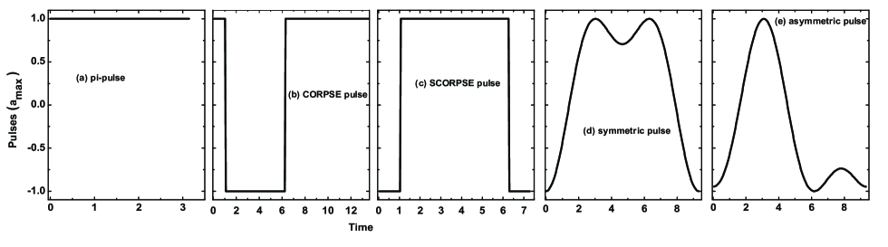
Figure 1: The form of designed pulses for (a) $\pi$, (b) CORPSE, (c) SCORPSE, (d) symmetric and (e) asymmetric. These pulses are under consideration to achieve fidelity recovery (or, minimize the error) in one qubit gate operation under random telegraph noise.

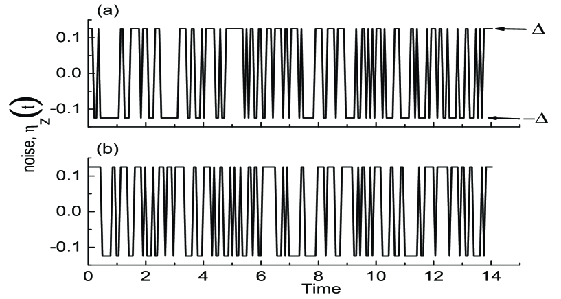
Figure 2: Simulations of random telegraph noise (RTN) as a function of time ($\hbar/a_{max}$) for the correlation time, $\tau_{c}$= 0.001($\hbar/a_{max}$). Note that the density of RTN jumps between $\pm\Delta$ is random which is shown in Fig.2(a) and (b). Here only two noises functions are shown for demonstration purpose but in a realistic simulation of finding error, 500 RTN trajectories have been chosen.)

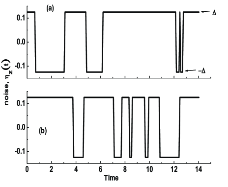
Figure 3: Same as to Fig. 2 but $\tau_{c}$=1($\hbar/a_{max}$). Notice that the jumps in RTN is significantly decreased as correlation time, $\tau_{c}$ increases. For large $\tau_{c}$ ($\approx$ 20($\hbar/a_{max}$)), RTN noise can be treated as a white noise.

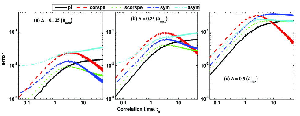
Figure 4: error (1-$\phi(\rho_{f},\rho_{0})$) vs noise correlation time, $\tau_{c}(\hbar/a_{max})$ for $\pi$ pulse (black, solid line), CORPSE pulse (red, dashed line), SCORPSE pulse (green, dotted line), symmetric pulse (blue, dotted line) and asymmetric pulse (cyan, dashed-dotted-dotted line). I chose $\Delta=0.125a_{max}$ as the amplitude of strength of the RTN noise.

In most cases, compared to coherent time, the dephasing time of qubits in presence of noise is reduced by several orders of magnitude due to coupling of qubits to the environment. The reduction of dephasing time depends on the specific dynamical coupling sequence from where the principle of quantum mechanics is inevitably lost. Therefore, one might need to decouple the qubits from the environment and may consider more robust topological method to preserve a quantum state against noise, enabling robust quantum memoryJing et al. (2015). Hence, to make quantum computers, one needs to find an efficient and experimentally feasible algorithm that overcome the issues of undesired interactions of qubits to the surrounding environment. Interactions of qubits to the surrounding environment destroy the quantum coherence that lead to generate errors and loss of fidelity. In quantum computing language, this phenomenon is called decoherence. For example, experimental observations reported that in GaAs quantum dots, decoherence time, $T_{2}^{\star}\approx 10ns$ and coherent time, $T_{1}\approx 0.1ms$, whereas for Si, $T_{2}^{\star}\approx 100ns$ and $T_{1}\approx 0.1ms$ Bluhm et al. (2011); Petta et al. (2005); Maune et al. (2012); Pla et al. (2012); Malinowski et al. (2018); Friesen et al. (2017); Martins et al. (2017); He et al. (2019); Geng et al. (2016); Liu et al. (2019); Throckmorton et al. (2017); Yang et al. (2018); Huang and Goan (2017). There are several possible ways to overcome the issues of decoherence, as for example, fidelity recovery by applying error-correcting codes, decoherence free subspace coding, noiseless subsystem coding, dynamical decoupling from hot bath, numerical design of pulse sequences, that is more robust to experimental inhomogeneities, and optimal control pulse based on Markovian master equation descriptions. Ofek et al. (2016); Michael et al. (2016); Brown et al. (2016); Reiserer et al. (2016); Lau and Plenio (2016); Liu et al. (2016); Castro et al. (2012); Wang et al. (2012); Jenei et al. (2019); Rudge and Kosov (2019); Motzoi et al. (2016); Dickel et al. (2018); Kurpiers et al. (2018); Campagne-Ibarcq et al. (2018) In Ref. Möttönen et al., 2006, authors provided a scheme of high fidelity recovery of qubits operating by $\pi$, CORPSE, and SCORPSE pulses in random telegraph noise but present work is different in that qubits operating by symmetric pulse shows the smallest error generation in the regime of small energy amplitudes of noise strength that has large noise correlation time. In addition, this paper investigates the interplay of these pulses acting in all three (x,y,z) directions while RTN still acts in z-direction and then identified the pulse sequences which provide less error on bit-flip qubits. Identifying pulse sequences that generate small error in small energy amplitudes of noise strength may be suitable for the experiments operating at low temperatures, whereas identifying pulse sequences that generate small error in large energy amplitudes of noise strength may be suitable for the experiments operating at high temperatures.

In this paper, I consider the design of several control pulses acting on a single bit-flip computational basis states in presence of noise. The present work seek to identify different regimes of operating parameters in the designed control pulses that eliminate the series of phase and dynamical errors and induce the recovery of high fidelities. The calculations are restricted to only eliminate the phase errors, which are more robust due to stochastic time-varying amplitudes, appear in the model Hamiltonian. More precisely, the designed pulses are $\pi$, CORSPE, SCORPSE, symmetric and asymmetric acting on a qubit in a random telegraph noise environment. Then checking the quantum gate errors at various noise correlation times as well as various energy amplitudes of noise strength as an indication of most efficient way to perform algorithm for quantum bit operations. The result of calculation shows that when the qubits are driven by pulses in the x-direction and the noises act in the z-direction then the symmetric pulse sequence along with small energy amplitude of noise strength, (i.e., $\Delta\approx 0.125\hbar/a_{max}$) induce less systematic errors over all the other pulses ($\pi$, CORPSE, SCORPSE and asymmetric pulses). Such error analysis in the qubits is useful for the laboratory experiments operating at low temperatures where one can correct the systematic errors in a more efficient way by designing additional quantum gates in a physical device . On the other hand, for the case of strong noise environments (i.e., energy amplitude of noise strength, $\Delta\approx 0.25\hbar/a_{max}$), may suitable for the experiments operating at room temperature, CORPSE pulse is the most efficient way to reduce the error. For a more general case, I consider the pulses acting in arbitrary x, y and z directions and show that when $\pi$ pulse acts in x-direction, CORPSE pulse acts in y-direction and SCORPSE pulse acts in z-direction in presence of arbitrary low and high temperature measurements noise condition, then such pulse sequences have large fidelity recovery and may consider better candidate for implementing in next generation electronic circuits design to minimize error.

The paper is organized as follows. In section II, I provide a theoretical description of the model Hamiltonian for a qubit operating under several control pulses in a random telegraph noise environment. In section IV, I analyze two main results: (i) qubits driven by a pulse in the x-direction and RTN noise acts in z-direction. (ii) individual pulse acts in the x,y and z-direction in the qubits and RTN still acts in the z-direction. Finally I conclude the results in Section V.

II Model Hamiltonian

The effective model Hamiltonian of a single qubit is written as Nielsen and Chuang (2000)

$$H(t)=\sum_{i\in\{x,y,z\}}\frac{1}{2}\left[a_{i}(t)+\eta_{i}(t)\right]\cdot\sigma_{i},$$ (1)

where $a_{i}(t)$ are the energy amplitude of the external control fields, $\eta_{i}(t)$ are the energy amplitude of the random environmental noise and $\sigma_{i}$ is the Pauli spin matrices. I further assumed that the designed control pulses are acting on all three x,y and z-directions while environmental noises are acting only in z-direction. Hence, the effective Hamiltonian (1) can be written as

$$H(t)=\frac{1}{2}\left[a_{x}(t)\sigma_{x}+a_{y}(t)\sigma_{y}+a_{z}(t)\sigma_{z}+\eta_{z}(t)\sigma_{z}\right].$$ (2)

Several designed pulses are shown in Fig. 1, which have the following sequences for energy amplitudes variations:

For $\pi$ pulse,

$$a_{\pi}(\theta)=a_{0},~{}~{}\mathrm{for}~{}~{}\theta\in\left[0,\pi\right].$$ (3)

For CORPPE pulse,

$$a_{C}(\theta) = a_{max},~{}~{}\mathrm{for}~{}~{}0<\theta<\frac{\pi}{3},$$ (4)

$$= -a_{max},~{}~{}\mathrm{for}~{}~{}\frac{\pi}{3}\leq\theta\leq 2\pi,$$

$$= a_{max},~{}~{}\mathrm{for}~{}~{}2\pi<\theta\leq\frac{13\pi}{3}.$$

For SCORPSE pulse,

$$a_{SC}(\theta) = -a_{max},~{}~{}\mathrm{for}~{}~{}0<\theta<\frac{\pi}{3},$$ (5)

$$= a_{max},~{}~{}\mathrm{for}~{}~{}\frac{\pi}{3}\leq\theta\leq 2\pi,$$

$$= -a_{max},~{}~{}\mathrm{for}~{}~{}2\pi<\theta\leq\frac{7\pi}{3}.$$

For symmetric pulse,

$$a(t)=\frac{\pi}{2}+\left(a-\frac{\pi}{2}\right)\cos{\left(\frac{2\pi t}{\tau}\right)}-a\cos{\left(\frac{4\pi t}{\tau}\right)},$$ (6)

$$a_{sym}(t)=\frac{a_{max}}{N_{1}}a(t)-a_{max},$$ (7)

where $a_{max}$=1, $a$ = 5.263022(1/$\tau$), $\tau$=9.325 and 1/$N_{1}$=0.8477 are integers.

For asymmetric pulse,

$$a_{asym}(t)=\frac{a_{max}}{N_{2}}\left[a(t)+b\sin{\left(\frac{2\pi t}{\tau}\right)}-\frac{b}{2}\sin{\left(\frac{4\pi t}{\tau}\right)}\right]-a_{max},$$ (8)

where $b$ = 17.850535(1/$\tau$) and 1/$N_{2}$=0.412 are integers. Above pulse sequences, which are plotted in Fig. 1, are used to drag the qubits in noisy environments to seek the recovery of the measurement of high fidelity quantum gates.

For random environmental noise, $\eta_{z}(t)$ changes randomly between two values $\eta(0)=\Delta$ and $\eta(0)=-\Delta$, where $\Delta$ is the energy amplitude of the strength of the noise. The environmental noise function is written as

$$\eta_{z}(t)=(-1)^{\Sigma_{i}\Theta\left(t-t_{i}\right)}\eta(0),$$ (9)

where $\Theta(t)$ is the heaviside step function, and $\tau_{c}$ is the correlation time. The jump time instants $t_{i}$ is expressed as

$$t_{i}=\sum_{j=1}^{i}-\tau_{c}ln(p_{j}),$$ (10)

where the random numbers $p_{i}\in(0,1)$ determine the sample trajectories of random telegraph noises. Two randomly generated environmental noise functions are shown in Fig. 2 and 3. For the simulations of fidelity measurement, $500$ randomly generated noise functions are chosen. As can be seen in Fig. 2, there are large density of random jump noises in the vicinity of zero correlation times, $\tau_{c}$. On the other hand, as $\tau_{c}$ increases, the density of random jump noises decreases that can be seen in Fig. 3.

Suppose the effective Hamiltonian (2) is acting only on the qubit. Hence, to find the system dynamics, average over different noise trajectories were chosen to find the system dynamics. Therefore, the density matrix of the dynamics of the system is written as

$$\rho(t)=lim~{}N\rightarrow\infty~{}\frac{1}{N}\sum_{k=1}^{N}U_{k}\rho_{0}U_{k}^{\dagger},$$ (11)

where $\rho_{0}$ is the initial state of the system and $\{U_{k}\}$ is the unitary time evolution of the qubit under the influence of control pulses (see Fig. 1) and randomly generated noise functions (see Fig. 2 and 3). The unitary time evolution operator is written as

$$U_{k}=\tau e^{{-i/2\hbar}\int_{0}^{t}d\tau\sum_{i\in\{x,y,z\}}\left[a_{i}(t)\cdot\sigma_{i}+\eta_{z}(t)\sigma_{z}\right]},$$ (12)

where $\tau$ is the time ordering parameter. Considering $\rho_{f}$ is the final state of the system then the fidelity for the system is given by

$$\phi=tr\{\rho_{f}^{\dagger}\rho_{T}\},$$ (13)

where $\rho_{T}$ is the final desired state of the qubit.

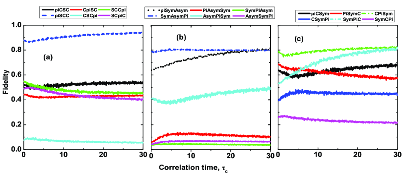
Figure 5: Bit flip fidelities, $\phi(\rho_{f},\rho_{0})$ vs noise correlation time, $\tau_{c}(\hbar/a_{max})$ for possible combinations of pulse sequences $\{a_{x}(t),a_{y}(t),a_{z}(t)\}$ in the Hamiltonian 2. Notice that the recovery of fidelity is the largest for $(a_{\pi}(t),a_{SC},a_{C})$ (Fig. 5(a), dashed line, blue), $(a_{\pi}(t),a_{sym},a_{Asym})$ (Fig. 5(b), dotted line, black) and $(a_{sym}(t),a_{Asym},a_{\pi})$ (Fig. 5(b),dashed-dotted line, blue). Similarly, the recovery of fidelity is the largest for $(a_{C}(t),a_{\pi}(t),a_{sym}(t))$ (Fig. 5(c). All other combinations of pulse sequences have small fidelities that may be useless for performing experiments. Here I chose $\Delta=0.125$.

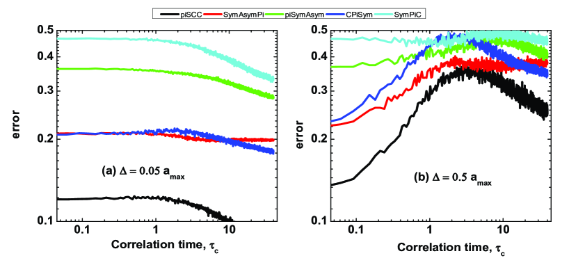
Figure 6: Bit flip fidelities, $\phi(\rho_{f},\rho_{0})$ vs noise correlation time, $\tau_{c}(\hbar/a_{max})$ for $\Delta=0.05$ (left panel) that is useful for low temperature measurements and $\Delta=0.5$ (right panel) that is useful for large temperature measurements. The combination of pulse sequences $\{a_{x}(t),a_{y}(t),a_{z}(t)\}$ in the Hamiltonian 2 $\pi$ is chosen same as to Fig. 5 but only consider those pulse sequences which has large fidelity recovery against noises.

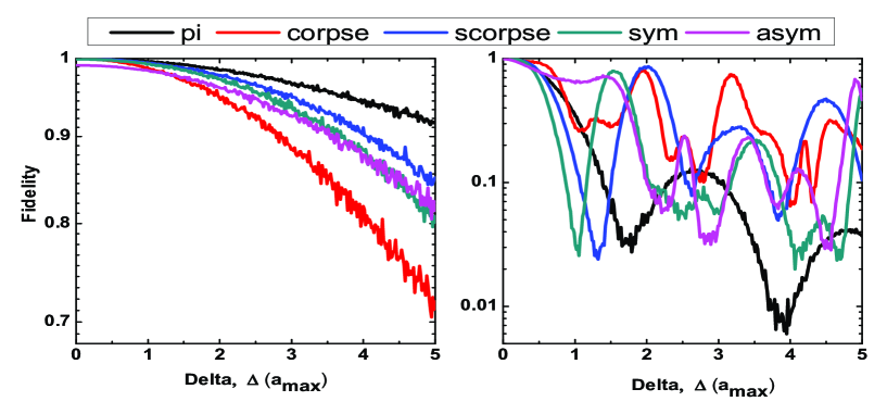
Figure 7: The pulse sequences are as same as to Fig. 4 (e.g., $a_{x}(t)$ is present but $a_{y}(t)$ and $a_{z}(t)$ are vanishing in the Hamiltonian 2) but $\tau_{c}=0.001$ (left figure) and $\tau_{c}=30$ (right figure). Notice that for small correlation time (left figure), fidelity recovery against noise strength is not possible due to the nature of the jumps in RTN (see Fig. 2). On the other hand, for large correlation time (right figure), fidelity recovery against noise strength is possible due to about no jumps in RTN which is the ideal case for white noise.

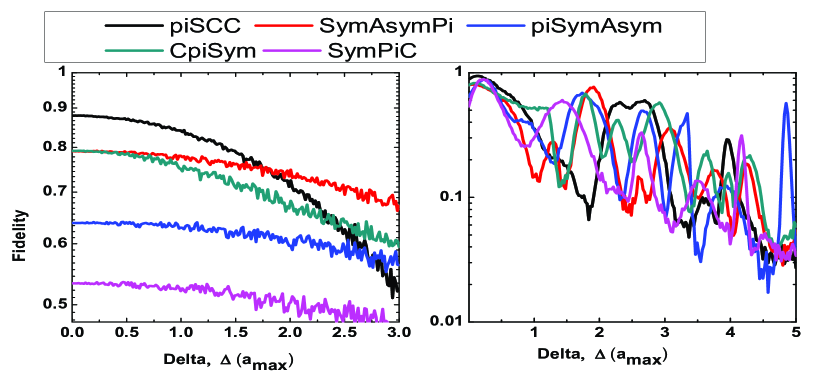
Figure 8: The pulse sequences are as same as to Fig. 6 (e.g., $a_{x}(t)$, $a_{y}(t)$ and $a_{z}(t)$ are all present in the Hamiltonian 2) but $\tau_{c}=0.001$ (left figure) and $\tau_{c}=30$ (right figure). Comparing Figs. 7 and 8, one finds that the performance of fidelity recovery is weak in Fig. 8 due to the possiblity of qubit interaction in all three x, y and z directions on the Bloch sphere.

III Computational Methods

I consider the bit flip computational basis states $|0>$ and $|1>$ as:

$$\rho_{0}=\left(\begin{array}[]{cc}0&0\\ 0&1\end{array}\right),~{}~{}~{}\rho_{f}=\left(\begin{array}[]{cc}1&0\\ 0&0\end{array}\right).$$

For the limiting case as the correlation time, $\tau_{c}\rightarrow 0$ and $\Delta\rightarrow\infty$, $\Delta^{2}\tau_{c}/2\equiv\hbar^{2}\Gamma$ remains finite value where $\Gamma$ is the decoherence time. In this case RTN model reduces to white noise. One may apply Markovian master equation in the model Hamiltonian to find the fidelity of the system Blum (1996). In this paper, I do not apply Markovian master equation instead write simulate the RTN trajectories numerically and then find the system dynamics by using Eq. (12). I have chosen $500$ RTN trajectories and express the density matrix of the system by a unitary quantum trajectory approach that is valid for all values of the correlation times $\tau_{c}$. Throughout the paper, I have chosen $\hbar=a_{max}=1$.

IV Results and Discussions

Considering $a_{y}(t)=a_{z}(t)=0$ in the Hamiltonian (2) and utilizing Eq. (13), the influence of $\pi$, CORSPE, SCORPSE, symmetric and assymetric pulses on the measurement of quantum error correction under random telegraph noises is shown in Figs. (4). Here $\Delta=0.125a_{max}$, $\Delta=0.25a_{max}$ and $\Delta=0.5a_{max}$ are chosen in (a),(b) and (c) of Fig. (4), respectively. In the regime of vanishing noise correlation time ($i.e.,\tau_{c}\rightarrow 0$), error is minimum which is shown in Fig. 4(a,b,c) for $\pi$ pulse followed by SCORPE, CORPE, symmetric and asymmetric pulses. The small error for $\pi$ pulse on the qubit operation is due to the fact that the single qubit under $\pi-$pulse does not have enough time to drift into the direction of densely populated random noise (see Fig. 2). Note that the noise function is very dense in the vicinity of zero correlation time (see Fig.2) while noise function has no jumps in the vicinity of infinite correlation time (e.g., density of noise jumps decreases as $\tau_{c}$ increases from Fig.2 to Fig.3). The energy amplitude of the noise functions rapidly changes its sign between $\pm\Delta$. Hence, in the vicinity of zero correlation time, the error is smaller or the fidelity is larger, to be about 99$\%$, for $\pi$ pulse than all the other pulses (e.g., SCORPSE, CORPSE, symmetric and asymmetric).

As a correlation time increases, the density of noises or the frequency of random jumps of noise functions decreases that can be seen in Figs. (2) and (3). Here I chose $\tau_{c}=0.001\hbar/a_{max}$ in Fig. 2 and ($\tau_{c}=1\hbar/a_{max}$) in Fig. (3). From Fig. 2 and Fig. 3, one can conclude that in the regime of sufficiently large noise correlation time ($i.e.,\tau_{c}\rightarrow\infty$), the frequency of random jumps of noise function $\eta(t)$ is significantly reduced, where noise function can be treated as a constant (no jumps or white nosie). The gate pulses acting on this regime with $\Delta=0.125$ quickly recover their lost fidelities except for $\pi$ and asymmetric pulses (see Fig. 4(a). However, for large value of $\Delta=0.5$, only CORPSE pulse has large fidelity recovery, which can be utilized to correct systematic time-independent errors. Since gate pulses (except $\pi$ pulse) change its amplitude between $\pm a_{max}$ with the variation of gate operation time, one can find the global minimum point at $\tau_{c}\approx 3\hbar/a_{max}$, from where the lost fidelity starts to recover.

I have plotted the error vs noise correlation time with $\Delta=0.25$ in Fig. 4(b) and with $\Delta=0.5$ in Fig. 4(c). Since $\Delta=$0.25 and 0.5 may consider a strong noisy environments, the qubit operation in this case may be suitable for gate operation at room temperature, the CORSPE pulse sequence recovers its lost fidelities more rapidly than other pulse sequences due to its large gate operation time. Hence in a very noisy environment, CORSPE pulse is only suitable candidate that correct the systematic errors. For a less noisy environment, i.e., $\Delta=0.125$ in Fig. 4(a) suitable for gate operation at low temperature, $\pi$ pulse in the regime of $\tau_{c}\rightarrow 0$ and the symmetric pulse sequences in the regime of $\tau_{c}\rightarrow\infty$ are the most suitable pulse to recover their lost fidelities.

Now I turn calculations for the pulses that act in x, y and z-directions while the RTN noises still act in the z-direction. The description of the qubits in this situations are well formulated by the Hamiltonian (2). I have tested interplay of several possible combinations of the pulse sequences $\{a_{x}(t),a_{y}(t),a_{z}(t)\}$ among $(a_{\pi}(t)$, $a_{C}(t)$, $a_{SC}(t)$, $a_{sym}(t)$ and $a_{asym}(t)$ in the Hamiltonian (2) and then plotted the fidelity vs correlation time in Fig 5. The results from this plots show that the pulses $a_{x}(t)$ represented by $a_{\pi}(t)$, $a_{y}(t)$ represented by $a_{SC}(t)$ and $a_{z}(t)$ represented by $a_{C}(t)$ has large value of fidelity shown in Fig. 5(a). Similarly, the pulses $a_{x}(t)$ represented by $a_{\pi}(t)$, $a_{y}(t)$ represented by $a_{sym}(t)$ and $a_{z}(t)$ represented by $a_{asym}(t)$ has large value of fidelity shown in Fig. 5(b)(dotted-line). In a similar way, the pulses $a_{x}(t)$ represented by $a_{sym}(t)$, $a_{y}(t)$ represented by $a_{asym}(t)$ and $a_{z}(t)$ represented by $a_{\pi}(t)$ has large value of fidelity shown in Fig. 5(b)(dotted-line). All the other combinations of pulse sequences has lower fidelity and may be useless for achieving less error in the low and high temperature measurements of bit-flip qubits.

In Fig. 6, I consider the same pulses that has large fidelity measurement in Fig. 5 but with different values of noise strength. Note that small value of noise strength, $\Delta$ is applicable for low temperature measurements while large value of $\Delta$ is applicable for high temperature measurements, probably room temperature. Here one find that when $\pi$ pulse acts in x-direction, CORPSE pulse acts in y direction and SCORPSE pulse acts in z-direction in presence of arbitrary low and high temperature measurements noise condition (i.e., small and large values of $\Delta$) have large fidelity recovery and may consider for implementing in next generation future electronic circuits design to minimize error.

In Fig. 7, I plot fidelity vs noise strength, $\Delta$, for the pulses acting only in the x-direction for correlation times, $\tau_{e}=0.001$ (left figure) and $\tau_{e}=30$ (right figure). Note that for $\tau_{e}=0.001$, the frequency of RTN jumps with respect to time is very large compared to almost no jumps for $\tau_{e}=30$. Hence fidelity recovery against noise strength is completely impossible for $\tau_{e}=0.001$ in Fig. 7 (left) but qubit driven by $\pi$ pulse in x-direction has large fidelity for large noise strength. Oscillations in fidelity can be seen for large RTN corellation time, $\tau_{e}=30$ in Fig. 7 (right) due to the fact that the RNT noise can act as a white noise. Here one finds that the fidelity recovery is faster for the case of qubit driven by symmetric pulse over all the other pulses (e.g., $\pi$, CORPSE, SCORPSE, and assymetric pulses). The data in Fig. 8 is the same as to Fig. 7 but qubits are driven by three different pulse sequences that has high fidelity against noises (also see Fig. 6). In Fig. 8, fidelity is inevitably lost compare to Fig. 7 because of possible interaction among qubit when these qubits are driven by pulse sequences on the Bloch sphere.

V Conclusion

In Fig. (4), I have demonstrated a possible way to minimize error and achieve high fidelity quantum gate operations using several bounded control pulses (e.g., $\pi$, CORPSE, SCORPE, symmetric and asymmetric pulses) acting on a one qubit system in presence of random telegraph noises. Here I have compared the errors for the qubits driven by the pulses discussed above. I conclude that in the limit of vanishing noise correlation time, $\pi$ pulse can be used for the measurement of achieving high fidelity due to its small gate operation time. In the limit of large correlation time, two pulses, namely symmetric pulse (Fig.4(a)) and CORPSE pulse (Fig.4(c), were identified to achieve recovery of high fidelity. More precisely, symmetric pulse (see Fig. 4(a)) provide large fidelity for the small energy amplitudes of noise strength which may be useful for the experiments that perform at low temperatures. On the other hand, CORPE pulse (see Fig. 4(b,c)) provide large fidelity for the large energy amplitudes of noise strength which may be useful for the experiments that perform at high temperatures. Finally, in Figs. 5 and 6, I have shown that when $\pi$ pulse acts in x direction, SCORPSE pulse acts in y direction and CORPSE pulse acts in z-direction in presence of arbitrary low and high temperature measurements noise conditions, large fidelity recovery can be achieved and may consider for implementing for next generation electronic circuits design to minimize error. In addition, oscillations in the fidelity measurement against noise strength for large correlation time (e.g., special case for white noise) is observed which is shown in Fig. 7 and 8.

VI Acknowledgements

This work is supported by Gordon State College under Faculty Development Program.

References

- Choi et al. (2000) M.-S. Choi, C. Bruder, and D. Loss, Physical review B 62, 13569 (2000).
- Burkard et al. (1999) G. Burkard, D. Loss, and D. P. DiVincenzo, Physical Review B 59, 2070 (1999).
- Hu and Sarma (2000) X. Hu and S. D. Sarma, Physical Review A 61, 062301 (2000).
- Koh et al. (2012) T. S. Koh, J. K. Gamble, M. Friesen, M. Eriksson, and S. Coppersmith, Physical review letters 109, 250503 (2012).
- Xiao et al. (2010) D. Xiao, M.-C. Chang, and Q. Niu, Reviews of modern physics 82, 1959 (2010).
- Prabhakar et al. (2010) S. Prabhakar, J. Raynolds, A. Inomata, and R. Melnik, Physical Review B 82, 195306 (2010).
- Prabhakar et al. (2014a) S. Prabhakar, R. Melnik, and L. L. Bonilla, Physical Review B 89, 245310 (2014a).
- Prabhakar et al. (2014b) S. Prabhakar, R. Melnik, and A. Inomata, Applied Physics Letters 104, 142411 (2014b).
- Vool et al. (2016) U. Vool, S. Shankar, S. Mundhada, N. Ofek, A. Narla, K. Sliwa, E. Zalys-Geller, Y. Liu, L. Frunzio, R. Schoelkopf, et al., Physical Review Letters 117, 133601 (2016).
- Lau and Plenio (2017) H.-K. Lau and M. B. Plenio, Physical Review A 95, 022303 (2017).
- Yoshihara et al. (2017) F. Yoshihara, T. Fuse, S. Ashhab, K. Kakuyanagi, S. Saito, and K. Semba, Nature Physics 13, 44 (2017).
- Clarke et al. (2016) D. J. Clarke, J. D. Sau, and S. D. Sarma, Physical Review X 6, 021005 (2016).
- Grünhaupt et al. (2019) L. Grünhaupt, M. Spiecker, D. Gusenkova, N. Maleeva, S. T. Skacel, I. Takmakov, F. Valenti, P. Winkel, H. Rotzinger, W. Wernsdorfer, et al., Nature materials 18, 816 (2019).
- Zhong et al. (2019) Y. Zhong, H.-S. Chang, K. Satzinger, M.-H. Chou, A. Bienfait, C. Conner, É. Dumur, J. Grebel, G. Peairs, R. Povey, et al., Nature Physics 15, 741 (2019).
- Kurpiers et al. (2019) P. Kurpiers, M. Pechal, B. Royer, P. Magnard, T. Walter, J. Heinsoo, Y. Salathé, A. Akin, S. Storz, J.-C. Besse, et al., Physical Review Applied 12, 044067 (2019).
- Xu et al. (2018) Y. Xu, W. Cai, Y. Ma, X. Mu, L. Hu, T. Chen, H. Wang, Y. Song, Z.-Y. Xue, Z.-q. Yin, et al., Physical review letters 121, 110501 (2018).
- Li et al. (2018) X. Li, Y. Ma, J. Han, T. Chen, Y. Xu, W. Cai, H. Wang, Y. Song, Z.-Y. Xue, Z.-q. Yin, et al., Physical Review Applied 10, 054009 (2018).
- Loss and DiVincenzo (1998) D. Loss and D. P. DiVincenzo, Physical Review A 57, 120 (1998).
- Golovach et al. (2004) V. N. Golovach, A. Khaetskii, and D. Loss, Phys. Rev. Lett. 93, 016601 (2004).
- Amasha et al. (2008) S. Amasha, K. MacLean, I. P. Radu, D. Zumbühl, M. Kastner, M. Hanson, and A. Gossard, Physical review letters 100, 046803 (2008).
- Balocchi et al. (2011) A. Balocchi, Q. Duong, P. Renucci, B. Liu, C. Fontaine, T. Amand, D. Lagarde, and X. Marie, Physical review letters 107, 136604 (2011).
- Jing et al. (2015) J. Jing, L.-A. Wu, M. Byrd, J. Q. You, T. Yu, and Z.-M. Wang, Phys. Rev. Lett. 114, 190502 (2015).
- Bluhm et al. (2011) H. Bluhm, S. Foletti, I. Neder, M. Rudner, D. Mahalu, V. Umansky, and A. Yacoby, Nature Physics 7, 109 (2011).
- Petta et al. (2005) J. R. Petta, A. C. Johnson, J. M. Taylor, E. A. Laird, A. Yacoby, M. D. Lukin, C. M. Marcus, M. P. Hanson, and A. C. Gossard, Science 309, 2180 (2005).
- Maune et al. (2012) B. M. Maune, M. G. Borselli, B. Huang, T. D. Ladd, P. W. Deelman, K. S. Holabird, A. A. Kiselev, I. Alvarado-Rodriguez, R. S. Ross, A. E. Schmitz, et al., Nature 481, 344 (2012).
- Pla et al. (2012) J. J. Pla, K. Y. Tan, J. P. Dehollain, W. H. Lim, J. J. Morton, D. N. Jamieson, A. S. Dzurak, and A. Morello, Nature 489, 541 (2012).
- Malinowski et al. (2018) F. K. Malinowski, F. Martins, T. B. Smith, S. D. Bartlett, A. C. Doherty, P. D. Nissen, S. Fallahi, G. C. Gardner, M. J. Manfra, C. M. Marcus, et al., Physical Review X 8, 011045 (2018).
- Friesen et al. (2017) M. Friesen, J. Ghosh, M. Eriksson, and S. Coppersmith, Nature communications 8, 15923 (2017).
- Martins et al. (2017) F. Martins, F. K. Malinowski, P. D. Nissen, S. Fallahi, G. C. Gardner, M. J. Manfra, C. M. Marcus, and F. Kuemmeth, Physical review letters 119, 227701 (2017).
- He et al. (2019) Y. He, S. Gorman, D. Keith, L. Kranz, J. Keizer, and M. Simmons, Nature 571, 371 (2019).
- Geng et al. (2016) J. Geng, Y. Wu, X. Wang, K. Xu, F. Shi, Y. Xie, X. Rong, and J. Du, Physical review letters 117, 170501 (2016).
- Liu et al. (2019) B.-J. Liu, X.-K. Song, Z.-Y. Xue, X. Wang, and M.-H. Yung, Physical Review Letters 123, 100501 (2019).
- Throckmorton et al. (2017) R. E. Throckmorton, E. Barnes, and S. D. Sarma, Physical Review B 95, 085405 (2017).
- Yang et al. (2018) X.-C. Yang, M.-H. Yung, and X. Wang, Physical Review A 97, 042324 (2018).
- Huang and Goan (2017) C.-H. Huang and H.-S. Goan, Physical Review A 95, 062325 (2017).
- Ofek et al. (2016) N. Ofek, A. Petrenko, R. Heeres, P. Reinhold, Z. Leghtas, B. Vlastakis, Y. Liu, L. Frunzio, S. Girvin, L. Jiang, et al., Nature 536, 441 (2016).
- Michael et al. (2016) M. H. Michael, M. Silveri, R. Brierley, V. V. Albert, J. Salmilehto, L. Jiang, and S. M. Girvin, Physical Review X 6, 031006 (2016).
- Brown et al. (2016) B. J. Brown, D. Loss, J. K. Pachos, C. N. Self, and J. R. Wootton, Reviews of Modern Physics 88, 045005 (2016).
- Reiserer et al. (2016) A. Reiserer, N. Kalb, M. S. Blok, K. J. van Bemmelen, T. H. Taminiau, R. Hanson, D. J. Twitchen, and M. Markham, Physical Review X 6, 021040 (2016).
- Lau and Plenio (2016) H.-K. Lau and M. B. Plenio, Physical Review Letters 117, 100501 (2016).
- Liu et al. (2016) B.-H. Liu, X.-M. Hu, J.-S. Chen, C. Zhang, Y.-F. Huang, C.-F. Li, G.-C. Guo, G. b. u. Karpat, F. F. Fanchini, J. Piilo, and S. Maniscalco, Phys. Rev. A 94, 062107 (2016).
- Castro et al. (2012) A. Castro, J. Werschnik, and E. K. Gross, Physical review letters 109, 153603 (2012).
- Wang et al. (2012) X. Wang, L. S. Bishop, J. Kestner, E. Barnes, K. Sun, and S. D. Sarma, Nature communications 3, 997 (2012).
- Jenei et al. (2019) M. Jenei, E. Potanina, R. Zhao, K. Y. Tan, A. Rossi, T. Tanttu, K. W. Chan, V. Sevriuk, M. Möttönen, and A. Dzurak, Phys. Rev. Research 1, 033163 (2019).
- Rudge and Kosov (2019) S. L. Rudge and D. S. Kosov, Phys. Rev. B 100, 235430 (2019).
- Motzoi et al. (2016) F. Motzoi, E. Halperin, X. Wang, K. B. Whaley, and S. Schirmer, Phys. Rev. A 94, 032313 (2016).
- Dickel et al. (2018) C. Dickel, J. J. Wesdorp, N. K. Langford, S. Peiter, R. Sagastizabal, A. Bruno, B. Criger, F. Motzoi, and L. DiCarlo, Phys. Rev. B 97, 064508 (2018).
- Kurpiers et al. (2018) P. Kurpiers, P. Magnard, T. Walter, B. Royer, M. Pechal, J. Heinsoo, Y. Salathé, A. Akin, S. Storz, S. Besse, J-C Gasparinetti, A. Blais, and A. Wallraff, Nature 558, 264 (2018).
- Campagne-Ibarcq et al. (2018) P. Campagne-Ibarcq, E. Zalys-Geller, A. Narla, S. Shankar, P. Reinhold, L. Burkhart, C. Axline, W. Pfaff, L. Frunzio, R. Schoelkopf, et al., Physical review letters 120, 200501 (2018).
- Möttönen et al. (2006) M. Möttönen, R. de Sousa, J. Zhang, and K. B. Whaley, Physical Review A 73, 022332 (2006).
- Nielsen and Chuang (2000) M. A. Nielsen and I. L. Chuang, Quantum Computation and Quantum Information (Cambridge University Press, Cambridge, England, 2000).
- Blum (1996) K. Blum, Density Matrix Theory and Applications (Plenum Press, New York, 1996).