Fractional advection-diffusion-asymmetry equation

Abstract

Fractional kinetic equations employ non-integer calculus to model anomalous relaxation and diffusion in many systems. While this approach is well explored, it so far failed to describe an important class of transport in disordered systems. Motivated by work on contaminant spreading in geological formations we propose and investigate a fractional advection-diffusion equation describing the biased spreading packet. While usual transport is described by diffusion and drift, we find a third term describing symmetry breaking which is omnipresent for transport in disordered systems. Our work is based on continuous time random walks with a finite mean waiting time and a diverging variance, a case that on the one hand is very common and on the other was missing in the kaleidoscope literature of fractional equations. The fractional space derivatives stem from long trapping times while previously they were interpreted as a consequence of spatial Lévy flights.

Fractional calculus is an old branch of mathematics that studies non-integer differential operators Oldham1974Fractional ; Samko1993Fractional ; Podlubny1999Fractional ; Meerschaert2012Stochastic . This method is used extensively to model anomalous diffusion and relaxation in a wide variety of systems Caputo ; SchneiderWyss ; MetzKlaf ; Sokolov . To recap consider the fractional diffusion equation Saichev ; Mainardi for the density of spreading particles ${\cal P}(x,t)$

$$\frac{\partial^{\beta}{\cal P}}{\partial t^{\beta}}=D_{\beta,\mu}{\nabla^{\mu}}{\cal P},$$ (1)

where $D_{\beta,\mu}$, with units ${\rm m}^{\mu}/\mbox{s}^{\beta}$, is a generalised diffusion constant. The fractional time and space derivatives are convolution operators that more intuitively are defined with their respective Laplace and Fourier transforms (see below). This equation, sometimes called the fractional diffusion-wave equation, reduces to the diffusion equation when $\beta=1,\mu=2$ and the wave equation for $\beta=2,\mu=2$. $\mu<2$ corresponds to long spatial jumps referred to as Lévy flights (LF), while $\beta<1$ to long dwelling times between jump events MetzKlaf . Originally this equation was derived using the continuous time random walk (CTRW) model Kotulski1995Asymptotic ; MetzKlaf ; Scalas ; Carioli ; Kutner ; Morales2017Stochastic ; Burioni2014Scaling . More recently the fractional diffusion equation with $\beta=1$ was derived for heat transport using models of interacting particles Kundu ; Dhar . Such fractional kinetic equations are used to describe the time of flight experiments of charge carriers in disordered systems where due to trapping $\beta<1,\mu=2$ Scher75 ; fracPRE and anomalous diffusion of cold atoms in optical lattices where the atom-laser interaction induces $\mu<2$ and $\beta=1$ Sagi ; KesBarPRL . Extensions that include external forces are well studied, within a framework referred to as the fractional Fokker-Planck equation FracPRL ; Marcin ; Deng2008Finite ; Henry1 , and distributed order fractional equations Chechkin2005Fractional ; Fedotov . For an extensive review see MetzKlaf .

Eq. (1) exhibits reflection symmetry and hence the packet of spreading particles is symmetric around its mean, if the initial condition density is localised. In disordered systems with fixed advection, symmetry breaking is found, and Eq. (1) is invalid. Such behavior is found throughout hydrology, for example, for tracer and contaminant spreading in heterogeneous media. For more than two decades, two opposing and competing frameworks were developed in this field. One approach advanced by Benson, Schumer, Meerschaert, and Wheatcraft (BSMW) Benson ; Shumer proposed that the mechanism for transport is controlled by non-local spatial jumps of the Lévy type MetzKlaf ; Zhang ; Kelly ; zhang2005mass . It was suggested that solute particles may experience long movements in high velocity flow paths, leading to such super diffusive behavior, possibly in the spirit of LFs in rotational flow Swinney . Importantly, since field observations exhibit non-symmetric shapes of the spreading packet of particles, the microscopic picture introduces skewed probability density function (PDF) of spatial jump lengths. This approach extensively promoted the use of non-symmetrical fractional space advection-diffusion equations for LFs, see Kelly for an overview.

The second approach uses what might be considered the opposite strategy. Instead of long non-local Lévy jumps in space, Berkowitz, Scher and co-workers Scher ; Berkowitz2002 ; Margolin ; Levy ; Berkowitz ; Edery ; Nissan ; Morales2017Stochastic showed that the CTRW framework with a power-law trapping time PDF is the key feature needed to explain the observed data. Physically this is the result of long trapping events in geometrically induced dead-ends found in strongly disordered porous media. Specifically, based on field experiments and extensive modelling, the trapping time PDF is $\psi(\tau)\sim\tau^{-(1+\beta)}$ and importantly in many cases $1<\beta<2$ Levy ; Berkowitz . Here the mean trapping time is finite, while the variance diverges. In this case Eq. (1) is certainly not valid. To see this consider a CTRW with a finite variance of jump lengths, so $\mu=2$ and then as mentioned if we take $\beta\to 2$ we get the wave equation, which is completely irrelevant for the transport under study. Thus, so far, the Scher-Berkowitz theoretical framework is based on a random walk picture Berkowitz2002 and not on a governing fractional advection-diffusion equation. Both the CTRW and the BSMW frameworks and the experiments in the field agree on one thing: advection-diffusion is anomalous and non-symmetric Burioni2013Rare ; Berkowitz ; Hou ; WanliPRR , however otherwise these schools promote widely different philosophies.

One goal of this letter is to promote a better understanding of the meaning of the fractional space derivatives in transport equations. As mentioned in the literature these are associated with LFs however we show here that they are actually related to the long-tailed PDF of trapping times, provided that $1<\beta<2$. The mentioned biased CTRW is known to exhibit super-diffusion $\langle(X-\langle X\rangle)^{2}\rangle\propto t^{3-\beta}$ Shlesinger1974Asymptotic however this as a stand alone does not imply a connection to LFs or fractional space kinetic equations. The first important conceptual step towards a unification of LFs and biased CTRW was given by Weeks, Urbach, and Swinney Weeks1998Anomalous ; Weeks1996Anomalous . In the presence of bias, an observer in a reference frame moving with the mean speed set by the advection, will view the power-law trapping times of the CTRW framework, as if the particle is performing large jumps in space. Our challenge is three fold. First to extend this idea into a fractional equation showing the role of fluctuations. Secondly, to develop a tool, capable of dealing with a wide variety of applied problems, ranging from calculations of breakthrough curves (see below), effect of time-dependent fields (omnipresent in field experiments) and different boundary conditions by far extending Burioni2013Rare ; Hou ; WanliPRR ; Shlesinger1974Asymptotic ; Weeks1998Anomalous ; Weeks1996Anomalous . In essence this framework is the continuum fractional diffusive description of a very large class of random walk processes. Finally, after deriving the fractional equation for the Berkowitz-Scher transport, we will be in the position to compare it to the BSMW LF method.

The fractional advection-diffusion-asymmetry equation (FADAE) investigated in this letter reads

$$\frac{\partial}{\partial t}{\cal P}=D{\partial^{2}\over\partial x^{2}}{\cal P}-V{\partial\over\partial x}{\cal P}+S{{\rm\partial}^{\beta}\over{\rm\partial}(-x)^{\beta}}{\cal P}.$$ (2)

The first two terms on the right-hand-side of Eq. (2) are the standard diffusion and drift terms, the last term is the modification we propose. The operator ${\rm\partial}^{\beta}/{\rm\partial}(-x)^{\beta}$ is a Riemann-Liouville fractional derivatives Samko1993Fractional ; MetzKlaf of order $1<\beta<2$; see the Appendix. The Fourier transform of this operator acting on some test function is ${\cal F}\left[{\rm d}^{\beta}g(x)/{\rm d}(-x)^{\beta}\right]=(-ik)^{\beta}\tilde{g}(k)$ where $\tilde{g}(k)$ is the Fourier transform of $g(x)$. In contrast to the spatial Riemann-Liouville derivatives in Eq. (2), the generalised Laplacian in Eq. (1) is symmetric Riesz derivatives Saichev , where ${\cal F}[\nabla^{\mu}g(x)]=-|k|^{\mu}\widetilde{g}(k)$. Further in Eq. (2) we have no fractional time derivatives and hence obviously it is very different from the standard fractional diffusion Eq. (1). Here $D$ describes normal diffusion, $V$ controls the drift, while $S$ is the symmetry breaking parameter. We now explain the meaning of Eq. (2) and its extensions.

When initially ${\cal P}(x,t)|_{t=0}=\delta(x)$, namely the packet of particles is localised on the origin, and when the transport coefficients are time-independent and for free boundary conditions, the solution is obtained using Fourier transform. Let $\tilde{{\cal P}}(k,t)$ be the Fourier pair of ${\cal P}(x,t)$ then Eq. (2) gives

$$\tilde{P}(k,t)=\exp\left[-Dk^{2}t-ikVt+S(-ik)^{\beta}t\right].$$ (3)

Thus the solution is a convolution of a Gaussian and a non-symmetric Lévy density Schneider1986Stable ; Zolotarev1986One ; Feller1971introduction ; Uchaikin2011Chance ; Padash2019First . These correspond to limit distributions of sums of independent identically distributed random variables described by thin and fat-tailed densities respectively. More specifically we denote $L_{\beta}(y)$ as the asymmetrical Lévy density whose Fourier transform is $\exp[(-ik)^{\beta}]$, and hence ${\cal P}(x,t)=L_{\beta}[x/(St)^{\beta}](St)^{-\beta}\bigotimes\exp[-(x-Vt)^{2}/4Dt]/\sqrt{4\pi Dt}$ where $\bigotimes$ is the convolution symbol WeylD ; Otiniano2013Stable .

Model. We treat the problem using the assumption that the particle will wait for some random time $\tau$ between two successive jumps. This is exactly the framework of the CTRW that describes a particle performing random independent steps $x$, determined by the PDF $f(x)$, and the waiting time $\tau$ distributed according to $\psi(\tau)$ Kotulski1995Asymptotic ; MetzKlaf ; Hou ; WanliPRR ; Shlesinger1974Asymptotic ; Weeks1998Anomalous ; Weeks1996Anomalous . All the waiting times and the jump lengths are independent. We consider, $\psi(\tau)\sim\beta(\tau_{0})^{\beta}\tau^{-1-\beta}$ and as mentioned $1<\beta<2$. The time scale $\tau_{0}$ together with the finite mean waiting time $\langle\tau\rangle=\int_{0}^{\infty}\tau\psi(\tau){\rm d}\tau$ is important. The probability of observing $N$ steps at time $t$ is Godreche ; WanliPRE

$$Q_{t}(N)\sim\frac{1}{(t/\bar{t})^{1/\beta}}L_{\beta}\left[\frac{N-t/\langle\tau\rangle}{(t/\bar{t})^{1/\beta}}\right]$$ (4)

with $\bar{t}=\langle\tau\rangle^{1+\beta}/[(\tau_{0})^{\beta}|\Gamma(1-\beta)|]$. This equation is valid for large times and large $N$, for example the mean number of jumps $\langle N\rangle\sim t/\langle\tau\rangle$ is large. Eq. (4) means that Lévy statistics are applicable for the shifted observable $N-\langle N\rangle$. For the jump length distribution $f(x)$, we assume that the mean size of the jumps is $a$ and the variance is $\sigma$. For example, in simulations below, the PDF of jump size is Gaussian

$$f(x)=\frac{1}{\sqrt{2\pi\sigma^{2}}}\exp\left[-\frac{(x-a)^{2}}{2\sigma^{2}}\right].$$ (5)

The parameter $a$ is the bias, and the mean position of the particle after $N$ steps, is $Na$ hence on average the packet of particles starting on the origin will be on $at/\langle\tau\rangle$. Clearly this modelling implies that we do not assume fat-tailed jump length distributions, unlike the LF picture in BSMW WeylD .

In CTRW the position of the particle after $N$ steps is $X=\sum_{i=1}^{N}x_{i}$, and thus it depends both on the microscopic displacements $x_{i}$ and the random number of steps $N$. By conditioning on a specific outcome of $N$ displacements, the PDF of finding the particle at $X$ at time $t$ is ${\cal P}_{{\rm CTRW}}(X,t)=\sum_{N=0}^{\infty}Q_{t}(N)P(X|N)$. We are interested in the long time limit since in this limit $N$ is large, hence we replace $P(X|N)$ with the Gaussian, and similarly replace $Q_{t}(N)$ with the Lévy distribution Eq. (4). Switching from summation to integration, in the long time limit we find

$${\cal P}_{{\rm CTRW}}(X,t)\sim\int_{0}^{\infty}L_{\beta}\left({N-t/\langle\tau\rangle\over(t/\bar{t})^{1/\beta}}\right){\exp\left(-{(X-aN)^{2}\over 2\sigma^{2}N}\right)\over\sqrt{2\pi\sigma^{2}N}(t/\bar{t})^{1/\beta}}{\rm d}N.$$ (6)

This idea is also known as the subordination of the spatial process $X$ by the temporal process for $N$ and is routinely considered in the literature for $\beta<1$, see Fogedby ; fracPRE . We already mentioned our intention to derive the spatial derivative usually associated with Lévy spatial jumps using the perfectly Gaussian jump statistics in space, and that is what we do next. In the long time limit, we find

$${\cal P}_{{\rm CTRW}}\sim\int_{-\infty}^{\infty}L_{\beta}(y){\exp\left\{-{\left[X-at/\langle\tau\rangle-ay(t/\bar{t})^{1/\beta}\right]^{2}\over 2\sigma^{2}t/\langle\tau\rangle}\right\}\over\sqrt{2\pi\sigma^{2}t/\langle\tau\rangle}}{\rm d}y.$$ (7)

Technically this limit is obtained with a change of variables to $\xi=(X-at/\langle\tau\rangle)/a(t/\bar{t})^{1/\beta}$ and $\xi$ is kept fixed while $t\to\infty$ WeylD . We now take the time derivative of the Fourier transform of Eq. (7) and find

$${\partial\tilde{{\cal P}}(k,t)\over\partial t}=-{\sigma^{2}\over 2\langle\tau\rangle}k^{2}\tilde{{\cal P}}(k,t)-ik{a\over\langle\tau\rangle}\tilde{{\cal P}}(k,t)+(-ik)^{\beta}{a^{\beta}\over\bar{t}}\tilde{{\cal P}}(k,t).$$ (8)

This is the Fourier representation of Eq. (2) when we identify the transport constants:

$$D={\sigma^{2}\over 2\langle\tau\rangle},\ V={a\over\langle\tau\rangle},\ S={a^{\beta}\over\bar{t}}.$$ (9)

The two formulas for $D$ and $V$ are standard relations in the theory of advection-diffusion. To summarize, the FADAE (2) describes the biased CTRW process and this has several consequences which are now discussed.

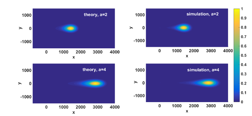
Figure 1: Packets of particles released from an origin in two-dimensions with $\beta=3/2$, time $t=200$ where the mean waiting time is $\langle\tau\rangle=0.3$ and $\tau_{0}=0.1$. The bias is pointing to the $x$ direction, while it is absent along the $y$ axis, and this creates packets distorted in the direction of the field. The symmetry breaking effect is visibly stronger as the bias level is increased. Here we show how simulations of the CTRW process and the analytical solutions of the FADAE nicely match. For theory we use Eq. (9) which gives $D=41.7,V=a/0.3$, and $S=a^{3/2}/0.44$ the bias $a$ is provided in the figure while in the $y$ direction $D=41.7$, and $S=V=0$. For further details on simulations see the Appendix, for example, a perfect agreement between theory and simulations without fitting, for one-dimensional CTRW.

The importance of bias. An interesting effect is that in the absence of bias, i.e. $a=0$ we get $S=0$, hence the anomaly is present only when we have advection. Since $S=0$ implies normal diffusion, in the case of weak advection the solution exhibits nearly normal behaviour even for very long times, an effect crucial for experiments. Further, Eq. (9) shows how the two transport coefficients $S$ and $V$ are generally not independent. To see this consider linear response theory. Then we have $a\sim F$ where $F$ is the external force field, and we have $V\sim F$ and $S\sim F^{\beta}$, a prediction that could be tested in experiments.

Packets in two dimensions. The fact that the asymmetry constant $S$ is bias-dependent leads to the following interesting prediction in two dimensions. Imagine the bias is directed in the $x$ direction, then the distortion of the packet of particles is found only along the $x$ axis. In other words the diffusion in the perpendicular $y$ direction will be perfectly normal. In the Appendix we extend our mathematical treatment of the problem to two dimensions. Here we present this effect graphically in Fig. 1, the asymmetrical oval like shape of the spreading packet is clearly visible, with the left tail broader than the right one. Similar experimental observations were reported in Levy ; Berkowitz2009shcer . The left tail, seen clearly in the figure, is due to trapping of particles far lagging behind the mean position of the packet and this as we showed is modeled with the asymmetry operator $\partial^{\beta}/\partial(-x)^{\beta}$ in Eq. (2). Thus the physical interpretation of the fractional space derivatives in FADAE should be made with care, as it does not necessarily mean that the process exhibits LFs.

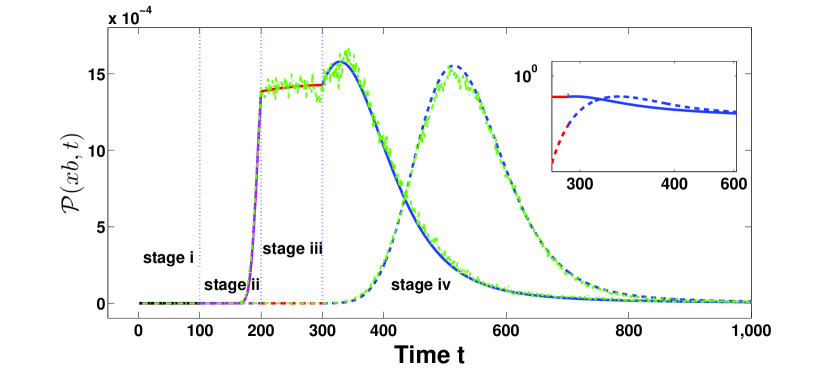
Figure 2: Particles are released on the origin at time zero and then the density on $x_{b}$ is recorded versus time. Such breakthrough curves present contaminant spreading from a source (say upper part of a stream) to some target on $x_{b}$, here $x_{b}=1800$. Here we present the solution of the FADAE and compare it with the CTRW simulations with $\beta=3/2$ without fitting. The bias $a$ is time-dependent, and as explained in the text, the dynamics has four stages as indicated in the graph, e.g. stage i), $0<t<100$ etc.

Temporal variations of the mean velocity $a/\langle\tau\rangle$ is often present in the real world and tested experimentally in Nissan . We explore this issue now using a time-dependant but piece wise constant bias $a(t)$ Nissan . Indeed in controlled experiments, the velocity $V$ can be modified, and then theoretical predictions can be tested in a non trivial setting. This example will demonstrate the power of the fractional framework, as it allows for a semi-analytical solution of the rather complex behaviour, and present physical effects related to the magnitude of the bias. We consider four stages of the transport Nissan : i) we use bias $a=1$ ii) we then sharply increase $a$ to a value $a=3.6$, then (iii) decrease the value then bias to a small number $a=0.09$, and finally (iv) return to the bias in state i). All along the second length scale $\sigma=5$ is fixed. The time lapses of each stage clearly indicated in Fig. 2 while the derivation of analytical results is left to the Appendix. Note that as we modify the bias $a$ we are effectively modifying $V$ and $S$ while $D$ remains fixed, see Eq. (9). The essential idea behind the analytical approach is that the final state of each stage serves as an initial condition to the spatial distribution of the next stage. In Fig. 2 (curve A) this analytical method is compared to numerical solution of the CTRW with $\beta=3/2$, finding excellent agreement. We also present the case of a constant time-independent $a=1$ (curve B). The concentration $P(x_{b},t)$ at some fixed $x_{b}$ presented in Fig. 2, is called a breakthrough curve and it is commonly observed in the field of contaminant spreading in Hydrology. Fig. 2 clearly demonstrates the excellent quantitive agreement between theory and simulation, in a regime of dynamics which is close to real real life experiments and far from trivial. Hence we are confident that our tool, the FADAE is a useful one.

Lévy flights and the interpretation of experiment. The CTRW process with long-tailed PDFs is an excellent model for transport in a wide variety of systems, for example porous media, hence the governing FADAE (2) is deeply related to transport in many physical systems MetzKlaf ; Kutner ; Hou ; Scher75 ; Bouchaud ; Andrea ; Scher2 ; PCCP . Still it is interesting to compare our approach to the fractional model of LFs that reads Benson ; remark

$${\partial{\cal P}_{{\rm LF}}\over\partial t}=-V{\partial{\cal P_{{\rm LF}}}\over\partial x}+K\left(q{\partial^{\mu}\over\partial(-x)^{\mu}}+p{\partial^{\mu}\over\partial x^{\mu}}\right){\cal P}_{{\rm LF}}$$ (10)

Clearly this equation is very different from ours, in fact in some sense it is more general as compared with Eq. (2), as it describes a general class of skewed processes with the phenomenological parameters $p$ and $q$. In zhang2005mass , authors fit experimental of contaminant data and report: $V=0.8~{}{\rm m/h}$, $D=0$, $\mu=1.51$, $K=2.8~{}{\rm m^{1.51}/h}$, $q=1$, and $p=0$ to match the breakthrough curves. Based on this one may naively interpret the data as stemming from a LF process. However, we realise that these parameters imply, based on our notation Eq. (2), a strong bias in the long time limit of CTRW. This highlights that the data are consistent with a CTRW with long-tailed trapping times. To summarize, using $p=0$ in Eq. (10) is consistent with both a LF picture promoted by BSMW and a CTRW with broad-tailed waiting times.

To distinguish between these two approaches one needs to analyse the trajectories of the process, not the packet of the spreading particles. More exactly, the CTRW approach and LFs method can give the same predictions for the positional distribution, but the interpretation that a model with fractional space derivatives always implies LFs is wrong. In that sense we claim that the two competing methods are identical (in some limit relevant to experiments) from the point of view of distributions but the particles trajectories widely differ.

Extensions with subordination. A key formula is the transformation Eq. (6). It shows how to transform a normal process to an anomalous one, for the case $1<\beta<2$ and as mentioned, this idea is called subordination. In Eq. (6) t is the laboratory time and $N$ is sometimes referred to as operational time. The idea is simple, $N$ which is actually the random number of steps in the process, is distributed according to Lévy statistics, as expected from the generalised central limit theorem. We then transform the Gaussian process in the operational time $N$ to the laboratory framework with what we call a Lévy transformation, see Eq. (6). This method, can be extended to include cases with different boundary conditions, different spatial dependent force fields, stochastic trajectories etc. and hence the mathematical approach we presented is versatile and far more general than what we considered here.

Mean square displacement. All along the manuscript we focus on the typical fluctuations of the process. The rare events influence the density $\mathcal{P}(x,t)$ in the vicinity of $x\simeq 0$ WanliPRR . Here Eq. (2) does not work. In that limit, the probability of finding these particles is very small, as expected for a biased process. In fact such a cutoff exists also for the diffusion equation, where the telegraph equation can be used to describe far tails of the density of particles. However, in the present case rare events control the behavior of the mean square displacement, which exhibits superdiffusion. It indicates that Eq. (2) cannot give a valid mean square displacement Hou ; WanliPRR , in this sense CTRWs are of course very different compared to LFs.

Summary. The FADAE (2) is controlled by three transport coefficients, $D$, $V$ and $S$, given in Eq. (9). This framework is valuable in many CTRW systems, ranging from the field of contaminant spreading and geophysics to transport random environments, for example, the quenched trap model Bouchaud ; Burov . What is remarkable is that the long-tailed PDF of trapping times, which for $0<\beta<1$ implies a fractional time derivative, is transplanted into a spatial space derivative when $1<\beta<2$. And long tailed PDFs of jump sizes, like in LFs, are not a basic requirement for fractional space operators in transport equations, rather these are related to Lévy statistics applied to the number of jumps in the process. In this sense we have provided a new physical and widely applicable interpretation of fractional space derivatives, within the context of fractional diffusion. More importantly, we provided a tool box with which one may analyse advection diffusion with different boundary conditions (with subordination) and with time-dependent fields.

Appendix A Mathematical background

Here we briefly discuss fractional derivatives, the non-symmetric stable probability density function, Eq. (7) in the main text, the infinite density that controls the rare fluctuations of $X$, the convolution used in the main text, and the general fractional advection-diffusion-asymmetry equation.

A.1 Riemann-Liouville derivatives

There are many excellent texts describing the long history and analytical properties of fractional derivatives, for example see Refs. Oldham1974Fractional ; Podlubny1999Fractional ; Meerschaert2012Stochastic . The fractional space derivatives operator $\frac{{\rm d}^{\beta}}{{\rm d}(-x)^{\beta}}$ used in the main text is now discussed. Here we focus on Riemann-Liouville derivatives Oldham1974Fractional ; remark . In real space, the (right) Riemann-Liouville derivative operator is defined through

$$\frac{{\rm d}^{\beta}}{{\rm d}(-x)^{\beta}}g(x)=\frac{(-1)^{n}}{\Gamma(n-\beta)}\frac{{\rm d}^{n}}{{\rm d}x^{n}}\int_{x}^{\infty}(y-x)^{n-\beta-1}g(y)\rm{d}y,$$ (11)

where $n$ is the smallest integer larger than $\beta$. While if the bottom limit of the integral is set to minus infinity, we have another related expression called left Riemann-Liouville derivatives

$$\frac{{\rm d}^{\beta}}{{\rm d}x^{\beta}}g(x)=\frac{1}{\Gamma(n-\beta)}\frac{{\rm d}^{n}}{{\rm d}x^{n}}\int_{-\infty}^{x}(x-y)^{n-\beta-1}g(y)\rm{d}y.$$ (12)

The mentioned operators have a simple expression under transforms since no initial values come into play. In Fourier space, the Riemann-Liouville derivative derivatives obey the following theorem Oldham1974Fractional ; remark

$$\left\{\begin{array}[]{ll}\displaystyle\mathcal{F}\left[\frac{{\rm d}^{\beta}}{{\rm d}(-x)^{\beta}}g(x)\right]=(-ik)^{\beta}\tilde{g}(k),&\hbox{}\\ \displaystyle\mathcal{F}\left[\frac{{\rm d}^{\beta}}{{\rm d}x^{\beta}}g(x)\right]=(ik)^{\beta}\tilde{g}(k),&\hbox{}\end{array}\right.$$ (13)

where we denote $\tilde{g}(k)$, $\tilde{g}(k)=\int_{-\infty}^{\infty}\exp(-ikx)g(x){\rm d}x$, as the Fourier transform of $g(x)$.

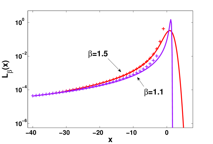
Figure 3: Plot of the Lévy distribution with $\beta=3/2~{}{\rm and}~{}\beta=1.1$, showing asymmetric far tails. The Lévy distribution is tabulated with Mathematica (see the solid lines) and the asymptotic behavior of the left tail, plotted by the symbols ‘$+$’, is obtained from Eq. (19) [the last line].

A.2 Non-symmetric Lévy distribution

As mentioned in the main text, in the long time limit, the number of jumps $N$ in the renewal process, shifted by its mean $\langle N\rangle$, follows the Lévy stable distribution, which is defined by

$$L_{\beta}(x)=\frac{1}{2\pi}\int_{-\infty}^{\infty}\exp(ikx)\exp[(-ik)^{\beta}]{\rm d}k.$$ (14)

If $0<\beta<1$, the above equation reduces to the one-sided Lévy distribution, namely $L_{\beta}(x)=0$ for $x>0$. In the literature, some authors prefer to use the characteristic function to define the Lévy distribution, for example, see Refs. Schneider1986Stable ; Zolotarev1986One ; Feller1971introduction ; Padash2019First , while we use the Fourier transform (the difference is simply a sign in front of $k$). Eq. (14) is plotted in Fig. 3 using Mathematica command, i.e., ${\rm PDF}{\rm[StableDistribution[}1,\beta,-1,0,{\rm Abs[Cos[Pi*}\beta/2]]^{1/\beta}],x]$; see also the inset in linear-linear scale. Rewriting Eq. (14), we have

$$L_{\beta}(x)=\frac{1}{\pi}\int_{0}^{\infty}\exp\left(k^{\beta}\cos\left(\frac{\pi\beta}{2}\right)\right)\cos\left(kx-k^{\beta}\sin\left(\frac{\pi\beta}{2}\right)\right){\rm d}k,$$ (15)

which can be used to plot the PDF of the Lévy distribution. We are interested in the decay of the far left and right tails, which are briefly presented below to emphasize the difference between them.

In the large deviation regime, namely $x$ is large, from Eq. (14) the saddle-point method yields

$$L_{\beta}(x)\sim\frac{\exp\left(-(\beta-1)(\frac{x}{\beta})^{\frac{\beta}{\beta-1}}\right)}{\sqrt{2\pi\beta^{-\frac{1}{\beta-1}}(\beta-1)x^{\frac{\beta}{\beta-1}}}},$$ (16)

which was found originally in Ref. Zolotarev1986One using other methods. This indicates that the right tail of the distribution decays as $\exp(-(\beta-1)(x/\beta)^{\frac{\beta}{\beta-1}})$, approaching zero rapidly.

Splitting the integral Eq. (14) into two parts at $k=0$ and changing variables $k^{{}^{\prime}}=k$ for the negative $k$, we have

$$L_{\beta}(x)=\mathcal{R}e\left[\frac{1}{\pi}\int_{0}^{\infty}\exp(-ikx)\exp((ik)^{\beta}){\rm d}k\right],$$ (17)

where $\mathcal{R}e[g(x)]$ means the real part of $g(x)$. Expanding the integrand $\exp[(ik)^{\beta}]$ in the right hand side of Eq. (17) as a Taylor series

$$\exp[(ik)^{\beta}]=\sum_{n=0}^{\infty}\frac{(-ik)^{\beta n}}{n!}=\sum_{n=0}^{\infty}\frac{1}{n!}(-ik)^{\frac{n+\frac{1}{\beta}-\frac{1}{\beta}}{\frac{1}{\beta}}},$$ (18)

and substituting Eq.  (18) into Eq.  (17), we get the asymptotic behavior of the left tail

$$\begin{split}L_{\beta}(x)&\sim\sum_{n=0}^{\infty}\mathcal{R}e\left[\exp\left(\frac{(n\beta+1)\pi}{2}\right)\Gamma(n\beta+1)\frac{i^{n\beta}}{n!(-x)^{n\beta+1}}\right]\\ &=\sum_{n=1}^{\infty}-\frac{\sin(n\beta\pi)\Gamma(n\beta+1)}{\pi n!(-x)^{n\beta+1}}\\ &\sim\frac{1}{\Gamma(-\beta)(-x)^{\beta+1}}\end{split}$$ (19)

with $x\to-\infty$. The well known leading term, i.e., the last line of Eq. (19), is plotted in Fig. 3 using the symbols ‘$+$’. Note that here we used method of stationary phase when calculating Eq. (19) from the integral Eq. (17). As shown in Fig. 3, we can see that two tails of the asymmetry Lévy distribution under study show different behaviors. The left one decays as a power law, i.e., $L_{\beta}(x)\sim(-x)^{-\beta-1}$ with $x\to-\infty$, tending to zero slowly if compared with the right one. This indicates that the variance of $x$ is infinity but the mean is finite. The exact expression of Lévy distribution, exists in terms of Fox function, which can also be expressed in the form of Mellin-Barnes type of integral. See Ref. Schneider1986Stable for a review. There are a number of cases of analytically expressible stable distribution, for example, when $\beta=3/2$, the Lévy distribution is related to Whittaker function Uchaikin2011Chance .

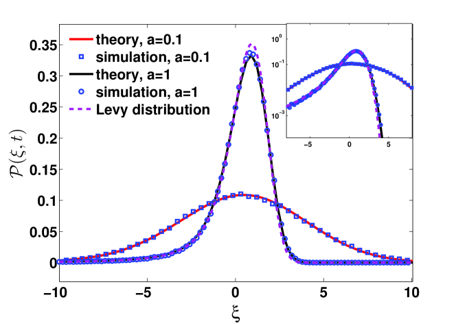
Figure 4: PDF of $\xi=(X-at/\langle\tau\rangle)/a(t/\bar{t})^{1/\beta}$ for various $a$ listed in figure. The symbols denote the simulation results obtained by averaging $10^{7}$ particles with $\beta=1.5$, $\tau_{0}=0.1$, $\sigma=1$ and $t=1000$. The corresponding theoretical theory plotted by solid lines is obtained from Eq. (7) in the main text by changing variable showing excellent fitting. When the bias is weak, the limiting law Eq. (20) plotted by the dashed line completely fails; see the simulations for $a=0.1$.

A.3 Derivation of Eq. (7)

In the Eq. (7) of the letter we used a subordination method. We now explain a step in the derivation. According to subordination form Eq. (6), we change variables according to $y=(N-t/\langle\tau\rangle)/(t/\bar{t})^{1/\beta}$ and find

$${\cal P}_{{\rm CTRW}}(X,t)\sim\int_{-\infty}^{\infty}L_{\beta}\left(y\right){\exp\left\{-{\left[X-at/\langle\tau\rangle-ay(t/\bar{t})^{1/\beta}\right]^{2}\over 2\sigma^{2}\left[t/\langle\tau\rangle+y(t/\bar{t})^{1/\beta}\right]}\right\}\over\sqrt{2\sigma^{2}\pi\left[t/\langle\tau\rangle+y(t/\bar{t})^{1/\beta}\right]}}{\rm d}y,$$

where the lower limit of the integration is found when $t\to\infty$. The typical fluctuations of the process, are found when $X-at/\langle\tau\rangle\sim a(t/\bar{t})^{1/\beta}$, and in this scaling regime, we finally find the law describing typical fluctuations, i.e., Eq. (7).

A.4 The Limit theorem and the infinite density.

The mean position of the walker in the long time limit is clearly $\langle X(t)\rangle\sim at/\langle\tau\rangle$, where $a$ is the mean displacement of each jump, and $t/\langle\tau\rangle$ is the average number of jumps. For convenience assume that $a>0$, so $\langle X(t)\rangle$ is positive. In the limit $t\to\infty$, it was rigorously shown that Kotulski1995Asymptotic ; Burioni2014Scaling ; WanliPRR

$$P(X,t)_{{\rm CTRW}}\sim{1\over l(t)}L_{\beta}\left({X-\langle X^{*}(t)\rangle\over l(t)}\right),$$ (20)

where $L_{\beta}(\cdot)$ represents the non-symmetrical Lévy stable law whose Fourier transform is $\exp[(-ik)^{\beta}]$ and $\langle X^{*}(t)\rangle$ is equal to $at/\langle\tau\rangle$. See the dashed line in Fig. (4). Here $l(t)=a(t/\overline{t})^{1/\beta}$ describing the width of the distribution is the typical length scale of the problem with $\overline{t}=\langle\tau\rangle^{1+\beta}/(\tau_{0})^{\beta}|\Gamma(1-\beta)|$. This equation while perfectly correct has several drawbacks which we wish to address. Firstly, the left tail of the density decays as a power law, which is a well known property of Lévy distribution. This naively implies that the mean square displacement is infinite, which is certainly not possible. An immediate consequence is that the mentioned super-diffusive effect discussed in the recent literature, is related to the non typical fluctuations. Thus it is not difficult to realize that this limit law has a cutoff, and this is solved recently in WanliPRR

$$\mathcal{P}(X,t)_{{\rm CTRW}}\sim\frac{(\tau_{0})^{\beta}t^{-\beta}}{a}\mathcal{I}_{\beta}(\eta)$$ (21)

with $0<\eta<1$, $\eta=1-(X/a)/(t/\langle\tau\rangle)$, and

$$\mathcal{I}_{\beta}(y)=\beta y^{-\beta-1}-(\beta-1)y^{-\beta}.$$

Eq. (21) is called the infinite density since the integration of Eq. (21) over $X$ diverges; see Figs. 6, 6, 8, and 8. Further discussion and simulations are presented in Ref. WanliPRR .

Secondly, Eq. (20) is independent of $\sigma$ which in many physical situations is not satisfactory. Let us consider a simple case, where the bias is weak and $t$ is finite. We have $a\ll\sigma$ and then expect that the variance of size of jumps is a key parameter, for example when $a=10^{-2}$, $\sigma=100$, $t=100$, we expect to get the Gaussian distribution. Further, in the context of active rheology and more generally single molecule experiments the number of jumps $N$ can be large (say $100-1000$) and the limit theorem which assumes $\langle N\rangle\to\infty$ is found to be a non-sensible description within the practical time range. As shown in Figs. 6 and 6, the limiting law Eq. (20) completely fails for small $a\ll\sigma$. With the growth of $a$, $P(\xi,t)$ approaches Eq. (20) slowly. Based on Eq. (21), the MSD reads

$$\langle x^{2}(t)\rangle-\langle x(t)\rangle^{2}\sim\frac{2a^{2}(\beta-1)(\tau_{0})^{\beta}|\Gamma(1-\beta)|}{\langle\tau\rangle^{3}\Gamma(4-\beta)}t^{3-\beta},$$ (22)

showing enhanced diffusion. Note that Eq. (22) can not be obtained from Eq. (2) in the main text since we used the typical fluctuations of $N$. In particular, if we are not interested in the mean square displacement, the rare events can be ignored; see Figs. 6 and 8.

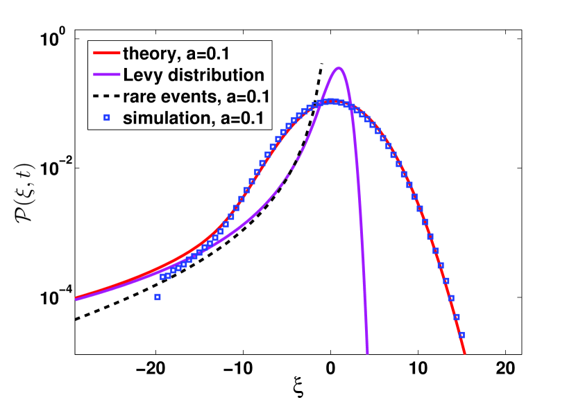
Figure 5: Simulations of the distribution of $\xi$ with the scaling $\xi=(X-\langle X^{*}(t)\rangle)/l(t)$ and $\beta=1.5$ compared with the analytical prediction Eq. (7) in the main text. Here we choose $t=10^{3}$, $\tau_{0}=0.1$, $\sigma=1$, $a=0.1$ and $10^{7}$ trajectories for simulations.

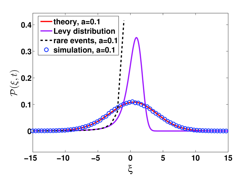
Figure 6: Same as Fig. 6 in linear-linear scale.

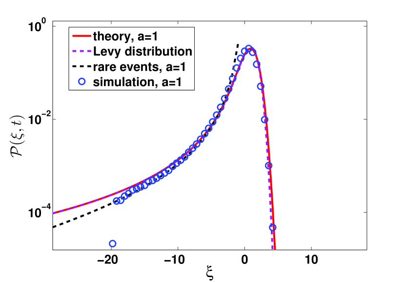
Figure 7: Same as Fig. 6 for $a=1$.

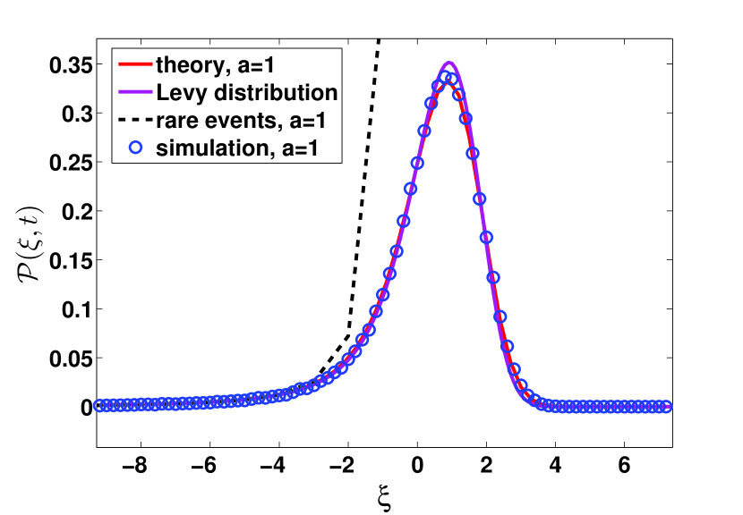
Figure 8: Same as Fig. 8 in linear-linear scale.

A.5 Convolution of Lévy and Gaussian distribution

Now let us consider the solution of the fractional advection-diffusion equation with an initial condition on the origin. As mentioned in the text the solution $\mathcal{P}(x,t)$ in one dimension is the convolution with respect to Lévy and Gaussian distributions

$$\mathcal{P}(x,t)=\int_{-\infty}^{\infty}\frac{1}{(St)^{1/\beta}}L_{\beta}\left(\frac{y}{(St)^{1/\beta}}\right)\exp\left(\frac{-(x-y-Vt)^{2}}{4Dt}\right)\frac{1}{\sqrt{4\pi Dt}}{\rm d}y.$$ (23)

Such a convolution is sometimes called the Voigt profile, see related discussions in Ref. Otiniano2013Stable . The scaling behavior of $\xi=(x-Vt)/(St)^{1/\beta}$ gives

$$\mathcal{P}(\xi,t)=\int_{-\infty}^{\infty}L_{\beta}\left(z\right)\underbrace{\exp\left(\frac{-(\xi-z)^{2}}{4Dt(St)^{-2/\beta}}\right)\frac{1}{\sqrt{4Dt}(St)^{-1/\beta}}}_{~{}}{\rm d}z.$$ (24)

Below we investigate two limits:

• When $\mathcal{Z}=4Dt(St)^{-2/\beta}\to 0$, i.e., $4Dt\ll(St)^{2/\beta}$, the term marked by under-brace in Eq. (24) reduces to a delta function using $\lim_{\epsilon\to 0^{+}}\exp(-z^{2}/(4\epsilon))/\sqrt{4\pi\epsilon}=\delta(z)$. Thus in the very long time limit the Lévy distribution describes the dynamics. This means that we can use the asymptotic behavior of Lévy distribution to study the properties of far tails of the distribution of the position.

• If $\mathcal{Z}\to\infty$ which is the short time limit, we have that the width of the Lévy distribution is narrow [see Eq. (23)] if compared with the width of Gaussian distribution. In this case, the Lévy distribution approaches to a “delta function”. As expected, we get the packet of spreading particles, following Gaussian distribution.

Notice that for a finite constant $\mathcal{Z}$ we use the integral Eq. (23) to show the solution of fractional advection-diffusion equation (2) in the main text.

To demonstrate these properties, in Fig. 9 we plot the solution $\mathcal{P}(x_{b},t)$ at site $x_{b}=Vt$ versus $t$, namely we focus on the probability of reaching the mean position. In other words, here $x_{b}$ is changing with time. Based on our setting in Fig. 9, we choose $D=41.7$, $V=3.3$, and $S=2.27$ which are transport constants of the fractional equation. If $t=10$, we have $\mathcal{Z}=26$. Thus we have $\mathcal{P}(x=V,t)\sim 1/\sqrt{4\pi Dt}$ for small $t$ since the packet of particles follows nearly Gaussian distribution. While, with the increase of the time $t$, as mentioned the Gaussian distribution fails, deviating from the solution of fractional advection-diffusion-asymmetry equation. Then at large times the solution using the Lévy stable law is valid, i.e., $\mathcal{P}(x_{b},t)\sim L_{\beta}(0)/(St)^{1/\beta}$. This transition is presented in Fig. 9.

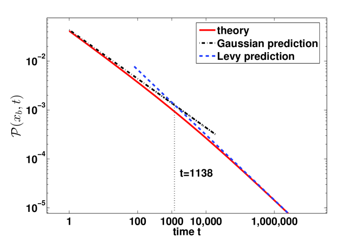
Figure 9: Concentration $P(x_{b},t)$ at changing site $x_{b}=Vt$ versus $t$. Solution of the fractional advection-diffusion equation, i.e., Eq. (23), is the solid line. The dash-dotted and the dashed lines are obtained from the corresponding Gaussian prediction valid for short times ($\mathcal{P}(x_{b},t)\sim 1/\sqrt{4\pi Dt}$) and Lévy prediction ($\mathcal{P}(x_{b},t)\sim L_{\beta}(0)/(St)^{1/\beta}$). Here we choose $\beta=1.5$, $D=41.7$, $V=3.3$, and $S=2.27$.

A.6 General fractional advection-diffusion-asymmetry equation

All along the main text, for example Eq. (5), we focus on the case when jump sizes have a finite non-zero mean and variance. We now further consider a general case, i.e., the displacement has a finite non-zero mean but infinite variance to extend the current Eq. (2) in the main text. In Fourier space, the displacement follows

$$\widetilde{f}(k)=\exp(-ika+(-ik)^{\gamma})$$ (25)

with $1<\gamma<2$, from which we get the probability of reaching $X$ after exactly $N$ steps

$$P(X|N)=\frac{1}{N^{1/\gamma}}L_{\gamma}\left(\frac{X-aN}{N^{1/\gamma}}\right).$$ (26)

If $N=1$, Eq. (26) reduces to $f(x)$ in real space. Utilizing Eqs. (4) and (26), we obtain

$$\mathcal{P}_{{\rm CTRW}}(X,t)\sim\frac{1}{(t/\bar{t})^{1/\beta}}\int_{0}^{\infty}L_{\beta}\left(\frac{N-t/\langle\tau\rangle}{(t/\bar{t})^{1/\beta}}\right)\frac{1}{N^{1/\gamma}}L_{\gamma}\left(\frac{X-aN}{N^{1/\gamma}}\right){\rm d}N.$$ (27)

Note that here $N$ is treated as a continuous variable. Changing variables of the above integral yields

$$\mathcal{P}_{{\rm CTRW}}(X,t)\sim\int_{-\infty}^{\infty}L_{\beta}(y)\frac{1}{(t/\langle\tau\rangle+y(t/\bar{t})^{1/\beta})^{1/\gamma}}L_{\gamma}\left(\frac{X-at/\langle\tau\rangle-ay(t/\bar{t})^{1/\beta}}{(t/\langle\tau\rangle+y(t/\bar{t})^{1/\beta})^{1/\gamma}}\right){\rm d}y$$ (28)

and performing Fourier transform with respect to $X$ leads to

$$\widetilde{\mathcal{P}}_{{\rm CTRW}}(k,t)\sim\exp\left(-ika\frac{t}{\langle\tau\rangle}+(-ik)^{\gamma}\frac{t}{\langle\tau\rangle}\right)\int_{-\infty}^{\infty}L_{\beta}(y)\exp\left(-ikay\left(\frac{t}{\bar{t}}\right)^{1/\beta}+(-ik)^{\gamma}y\left(\frac{t}{\bar{t}}\right)^{1/\beta}\right){\rm d}y.$$ (29)

We are interested in the statistics of $X$ in the long time limit. For small $k$, Eq. (29) reduces to

$$\widetilde{\mathcal{P}}_{CTRW}(k,t)\sim\exp\left(-ika\frac{t}{\langle\tau\rangle}+(-ik)^{\gamma}\frac{t}{\langle\tau\rangle}+(-ik)^{\beta}\frac{a^{\beta}t}{\bar{t}}\right).$$ (30)

Thus, the corresponding general fractional advection-diffusion equation reads

$$\frac{\partial}{\partial t}\mathcal{P}=-\frac{a}{\langle\tau\rangle}\frac{\partial}{\partial x}\mathcal{P}+\frac{1}{\langle\tau\rangle}\frac{\partial^{\gamma}}{\partial(-x)^{\gamma}}\mathcal{P}+\frac{a^{\beta}}{\bar{t}}\frac{\partial^{\beta}}{\partial(-x)^{\beta}}\mathcal{P}.$$ (31)

In particular, when $\gamma=2$ in Eq. (31), we get Eq. (2) in the main text which describes the case of Gaussian displacements. It can be seen that the method given in the main text is valid for a vast number of models. As mentioned before, we have two ways to derive Eq. (31). The first approach is from the well-known Lévy flight, i.e., the asymptotic displacement captures a non-zero mean and an infinite variance with two heavy tails. The second way dealing with Eq. (31) is a CTRW framework, where the waiting time has a fat tail with a finite mean and an infinite variance, and the distribution of the displacement has only one fat tail. It can be seen that the positional distribution for both approaches is the same. The interesting point is that the types of particles’ trajectories behind Eq. (31) are totally different, see the discussion in the main text.

Appendix B Fractional advection-diffusion-asymmetry equation in two dimensions

Now we study the advection-diffusion equation in two dimensions and present a generalization of Eq. (2) in the main text. We further use a CTRW formalism in two dimensions to explain the meaning of the equation.

Motivated by previous studies of the CTRW, we consider here the probability density function capturing a fat tail

$$\begin{array}[]{ll}\psi(\tau)=\left\{\begin{split}&0,&\hbox{$\tau<\tau_{0}$;}\\ &\beta\frac{(\tau_{0})^{\beta}}{\tau^{1+\beta}},&\hbox{$\tau\geq\tau_{0}$}\end{split}\right.\end{array}$$ (32)

with $1<\beta<2$. Clearly, the waiting time $\tau$ has an finite mean $\langle\tau\rangle$ but a infinite variance. In our simulations, we choose $\tau_{0}=0.1$ and $\beta=3/2$ and hence $\langle\tau\rangle=0.3$. Thus, if the observation time $t=1000$, the average number of renewals is $\langle N\rangle\sim t/\langle\tau\rangle\simeq 3333$.

The joint PDF of jump length follows

$$\begin{split}f(x,y)&=\frac{1}{\sqrt{2(\sigma_{x})^{2}\pi}}\exp\left(-\frac{(x-a_{x})^{2}}{2(\sigma_{x})^{2}}\right)\times\frac{1}{\sqrt{2(\sigma_{y})^{2}\pi}}\exp\left(-\frac{y^{2}}{2(\sigma_{y})^{2}}\right),\end{split}$$ (33)

where $a_{x},~{}\sigma_{x}$, $\sigma_{y}\neq 0$ are constants. This indicates that the drift is only in $x$ direction. In double Fourier spaces, $x\to k_{x}$ and $y\to k_{y}$, we get

$$\widetilde{f}(k_{x},k_{y})=\exp\left(-ik_{x}a_{x}-\frac{1}{2}(\sigma_{x})^{2}(k_{x})^{2}-\frac{1}{2}(\sigma_{y})^{2}(k_{y})^{2}\right),$$ (34)

which gives the PDF of finding the particle on site $(X,Y)$ after exactly $N$ steps by taking the inverse Fourier transform of $\widetilde{f}^{N}(k_{x},k_{y})$. Restarting from Eq. (7) in the main text, in the long time limit, $\mathcal{P}(X,Y,t)_{{\rm CTRW}}$ becomes

$$\mathcal{P}(X,Y,t)_{{\rm CTRW}}\sim\int_{-\infty}^{\infty}L_{\beta}(z)\frac{\exp\left(-\frac{(X-\frac{a_{x}t}{\langle\tau\rangle}-a_{x}z(\frac{t}{\overline{t}})^{1/\beta})^{2}}{2(\sigma_{x})^{2}\frac{t}{\langle\tau\rangle}}\right)}{\sqrt{2\pi(\sigma_{x})^{2}\frac{t}{\langle\tau\rangle}}}\frac{\exp\left(-\frac{Y^{2}}{2(\sigma_{y})^{2}\frac{t}{\langle\tau\rangle}}\right)}{\sqrt{2\pi(\sigma_{y})^{2}\frac{t}{\langle\tau\rangle}}}{\rm d}z.$$ (35)

Taking double Fourier transforms with respect to $X$ and $Y$, respectively, we get a useful expression

$$\widetilde{P}(k_{x},k_{y},t)_{{\rm CTRW}}\sim\exp\left(-(k_{y})^{2}(\sigma_{y})^{2}\frac{t}{2\langle\tau\rangle}-(k_{x})^{2}(\sigma_{x})^{2}\frac{t}{2\langle\tau\rangle}-ia_{x}k_{x}\frac{t}{\langle\tau\rangle}+\left(-ia_{x}k_{x}\left(\frac{t}{\overline{t}}\right)^{1/\beta}\right)^{\beta}\right).$$ (36)

Note that if $k_{x}=k_{y}=0$, we can check that $\mathcal{P}(X,Y,t)_{{\rm CTRW}}$ is normalized for any time $t$. Similar to the calculation in the main text, we take the time derivative of this solution, perform the inverse Fourier transform and then find using Eqs. (13) and (36)

$$\frac{\partial}{\partial t}\mathcal{P}(x,y,t)=\frac{(\sigma_{y})^{2}}{2\langle\tau\rangle}\frac{\partial^{2}}{\partial y^{2}}\mathcal{P}(x,y,t)+\frac{(\sigma_{x})^{2}}{2\langle\tau\rangle}\frac{\partial^{2}}{\partial x^{2}}\mathcal{P}(x,y,t)-\frac{a_{x}}{\langle\tau\rangle}\frac{\partial}{\partial x}\mathcal{P}(x,y,t)+\frac{(a_{x})^{\beta}}{\overline{t}}~{}\frac{\partial^{\beta}}{\partial(-x)^{\beta}}\mathcal{P}(x,y,t).$$ (37)

This is the fractional advection-diffusion equation in two dimensions, where the symmetry breaking takes place only in the $x$ direction, where the bias is pointing to. The solution of the above equation is plotted in Fig. 1 in the main text showing the packet of spreading particles. In this figure, we denote $a$ as $a_{x}$ to simplify our expression. Note that Eq. (37) is not just valid for Gaussian displacement given in Eq. (35) but the displacement should have a finite mean and a finite variance. In particular, when $a_{x}=0$, the above equation reduces to the classical diffusion equation. Clearly, the marginal density $\mathcal{P}(x,t)$ is the corresponding one dimensional solution Eq. (7) in the main text.

Appendix C Breakthrough curves

Here the aim is to use the fractional advection-diffusion-asymmetry equation found in the main text to predict breakthrough curves. For that, the first step is to obtain $\mathcal{P}(x,t)$ from Eq. (2) with time-dependent bias and then use it to compare with simulations of CTRW breakthrough curves.

C.1 Theory of propagator with time-dependent but piece wise constant bias

Motivated by Nissan , we consider time-dependent bias determined by four stages. We suppose that the rapid injection of particles is done immediately after starting observing the process. In other words, the initial condition of the particle is $\mathcal{P}(x,t=0)=\delta(x)$. As mentioned in the main text we simulate the spreading of the particles consisting of four states: (i) after the injection of the particles, they are moving with a constant bias which is determined by $a_{1}=a$, (ii) in the time interval $t_{1}<t<t_{2}$, we increase the bias sharply to $a_{2}=4a\gamma/(\gamma+1)$ with $\gamma\geq 1/3$, (iii) decrease the bias abruptly to $a_{3}=a/(2/3+\gamma)$, and (iv) then finally starting at $t_{3}$ return to the state (i) with $a_{4}=a$. Here $\gamma$ is a constant that controls the strength of bias or the average of “velocity”. In particular, when $\gamma=1/3$, and hence all the states mentioned above are the same. In Fourier space, the initial condition satisfies $\widetilde{\mathcal{P}}(k,0)=1$. In view of the special expression of $\widetilde{\mathcal{P}}(k,t)$, $\widetilde{\mathcal{P}}(k,t)$ for different states can be cast as

$$\widetilde{\mathcal{P}}(k,t)=\left\{\begin{array}[]{ll}\exp(-c_{11}k^{2}-ic_{12}k+c_{13}(-ik)^{\beta}),&\hbox{$0<t\leq t_{1}$;}\\ \exp(-c_{21}k^{2}-ic_{22}k+c_{22}(-ik)^{\beta}),&\hbox{$t_{1}<t\leq t_{2}$;}\\ \exp(-c_{31}k^{2}-ic_{32}k+c_{33}(-ik)^{\beta}),&\hbox{$t_{2}<t\leq t_{3}$;}\\ \exp(-c_{41}k^{2}-ic_{42}k+c_{43}(-ik)^{\beta}),&\hbox{$t_{3}<t$}\end{array}\right.$$ (38)

with

$$c_{m1}=\left\{\begin{array}[]{ll}t\frac{\sigma^{2}}{2\langle\tau\rangle},&\hbox{$m=1$;}\\ t\frac{\sigma^{2}}{2\langle\tau\rangle},&\hbox{$m=2$;}\\ t\frac{\sigma^{2}}{2\langle\tau\rangle},&\hbox{$m=3$;}\\ t\frac{\sigma^{2}}{2\langle\tau\rangle},&\hbox{$m=4$,}\end{array}\right.$$ (39)

$$c_{m2}=\left\{\begin{array}[]{ll}a_{1}\frac{t}{\langle\tau\rangle},&\hbox{$m=1$;}\\ \left[a_{1}t_{1}+a_{2}(t-t_{1})\right]\frac{1}{\langle\tau\rangle},&\hbox{$m=2$;}\\ \left[a_{1}t_{1}+a_{2}(t_{2}-t_{1})+a_{3}(t-t_{2})\right]\frac{1}{\langle\tau\rangle},&\hbox{$m=3$;}\\ \left[a_{1}t_{1}+a_{2}(t_{2}-t_{1})+a_{3}(t_{3}-t_{2})+a_{4}(t-t_{3})\right]\frac{1}{\langle\tau\rangle},&\hbox{$m=4$,}\end{array}\right.$$ (40)

and

$$c_{m3}=\left\{\begin{array}[]{ll}a_{1}^{\beta}t\frac{1}{\overline{t}},&\hbox{$m=1$;}\\ \left[a_{1}^{\beta}t_{1}+a_{2}^{\beta}(t-t_{1})\right]\frac{1}{\overline{t}},&\hbox{$m=2$;}\\ \left[a_{1}^{\beta}t+a_{2}^{\beta}(t_{2}-t_{1})+a_{3}^{\beta}(t-t_{2})\right]\frac{1}{\overline{t}},&\hbox{$m=3$;}\\ \left[a_{1}^{\beta}t_{1}+a_{2}^{\beta}(t_{2}-t_{1})+a_{3}^{\beta}(t_{3}-t_{2})+a_{4}^{\beta}(t-t_{3})\right]\frac{1}{\overline{t}},&\hbox{$m=4$.}\end{array}\right.$$ (41)

Here recall that $\bar{t}=\langle\tau\rangle^{1+\beta}/[(\tau_{0})^{\beta}|\Gamma(1-\beta)|]$ which is fixed, since in our simulations of the CTRW we only change the bias. The main idea of the analytical calculation is that the final position of each stage will be treated as an “initial condition” for the next stage. In particular, if $a_{1}=a_{2}=a_{3}=a_{4}$, Eq. (38) reduces to a constant bias case calculated in the main text. For the four-stage process, from Eq. (38) the solution is of the form

$$\mathcal{P}(x,t)=\int_{-\infty}^{\infty}\frac{1}{\sqrt{4\pi c_{m1}}}\exp\left[-\frac{(x-y-c_{m2})^{2}}{4c_{m1}}\right]\frac{1}{(c_{m3})^{1/\beta}}L_{\beta}\left[\frac{y}{(c_{m3})^{1/\beta}}\right]{\rm d}y$$ (42)

with $m=1,2,3,4$ being the number of the state. This is plotted in Fig.  10 for different times $t$. Note that when $0<t<t_{1}$, the solution Eq. (42) reduces to Eq. (7) in the main text.

C.2 Breakthrough curves

As mentioned in the main text breakthrough curves are measured considering a source that passes through the absorbent fixed bed sample, which is a method to analyze the adsorption properties of tracers in porous materials. An example of experiments is the transport through layers of different media, see Refs. Berkowitz2009shcer ; Nissan . With Eq. (42) we constructed the analytical solution presented in Fig. 2 of the main text. In Fig. 2 we use $\gamma=10$ for curve A, and further choose $a=1$, so there we have in the four stages $a=\{1,3.6,0.09,1\}$. Curve B in Fig. 2 corresponds to the case $\gamma=1/3$, where we get $a=\{1,1,1,1\}$. For the time interval of each state we use $t_{1}=t_{2}-t_{1}=t_{3}-t_{2}=100$ and $t-t_{3}=700$. Note that the detection wall is set on $x_{b}=1800$. In addition to Fig. 2 in the main text here we present results for the density with $t_{1}=t_{2}-t_{1}=t_{3}-t_{2}=10$ as this shows the quick convergence to our theory; see Fig. 11. Here the time interval is $10$ for the first three stages, given that $\langle\tau\rangle=0.3$ we have roughly $33$ steps in each of the first three time intervals. The figure illustrates that even for these relatively short time intervals the approximation works nicely.

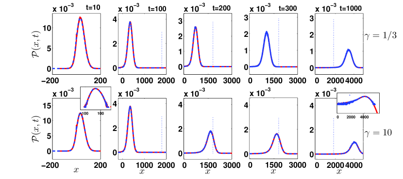
Figure 10: Simulations of propagators for different states with theoretical predictions Eq. (42). Waiting times of particles are drawn from Eq. (32) and displacements generated according to $f(x)=\exp(-(x-a)^{2}/2\sigma^{2})/\sqrt{2\pi\sigma^{2}}$, where $a$ is time dependent obtained for $\gamma=1/3~{}({\rm the~{}first~{}row}),~{}10$ (the second). The red solid lines are the theory and the blue dashed lines are the simulation results generated from $2\times 10^{6}$ trajectories. The time interval of the first three states is $100$ and the total time of the last state is $700$. Note that here it is not easy to see the asymmetry of the packet of spreading particles in a linear-linear plot for large $t$, at least this figure can be treated as an optical illusion. However, semi-log scales are presented to show the symmetric properties of the packet and the heavy tail; see the left and the right insets. The parameters are $\beta=3/2$, $\tau_{0}=0.1$, and  $\sigma=5$, which are the same as Fig. 2 in the main text.

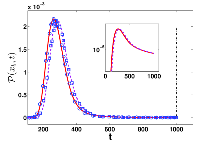
Figure 11: A plot of breakthrough curves for a weak bias. Here we choose $\beta=3/2$, $\tau_{0}=0.1$, $t_{1}=10$, $t_{2}=20$, $t_{3}=30$, $t=1000$, $\gamma=1/3$ (solid lines), and $\gamma=10$ (dashed lines). The detection wall for breakthrough curves is $x_{b}=10^{3}$; see the dash-dotted line. For both cases, after reaching a peak, we see a slow decay of the far right tail to zero, if compared to the left one (see the inset). Clearly the theoretical predictions Eq. (38) (the solid and the dashed lines) are consistent with simulations results plotted by the symbols.

Similarly, one can deal with time-dependent bias in two dimensions using Eq. (36) like Eq. (38). In Fig. 12, the time-dependent bias in two dimensions is investigated and the asymmetry packet with respect to $x$ is clearly observed. Here we have the drift in the $x$ direction and no bias in the $y$ direction, i.e.,

$$a_{x}=\left\{\begin{array}[]{ll}a,&\hbox{$0<t\leq t_{1}$;}\\ \frac{4a}{\gamma+1},&\hbox{$t_{1}<t\leq t_{2}$;}\\ \frac{a}{\gamma+\frac{2}{3}},&\hbox{$t_{2}<t\leq t_{3}$;}\\ a,&\hbox{$t_{3}<t$.}\end{array}\right.$$ (43)

It can be seen that Figs. 10 and 12 are complementary and yield a better understanding of breakthrough curves and the asymmetric packets of spreading particles.

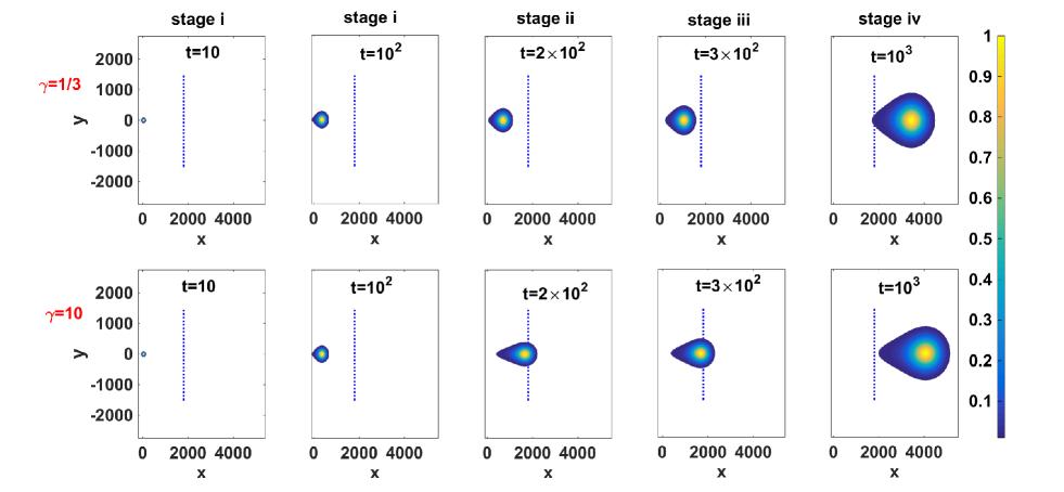
Figure 12: Theoretical prediction $\mathcal{P}(x,y,t)/\mathcal{P}_{\max}$ showing spatial contour maps under the time-dependent bias in two dimensions, where $\mathcal{P}_{\max}=\max_{x,y\in(-\infty,\infty)\times(-\infty,\infty)}(\mathcal{P}(x,y,t))$. The colorbar represents the relative concentration, $\mathcal{P}(x,y,t)/{\mathcal{P}_{\max}}$. Here fours stages are $0<t<100$, $100<t<200$, $200<t<300$, and $300<t<1000$. The joint PDF of displacements follows Eq. (33) with a changing $a_{x}$, namely we have $a_{x}=\{1,3.6,0.09,1\}$  ($a_{x}=\{1,1,1,1\}$) when $\gamma=10$  ($\gamma=1/3$); see Eq. (43). The theoretical results are obtained from Eqs. (38) and (36), namely $\mathcal{P}(x,y,t)$ factorizes into a product of Eq. (42) and $\exp(-y^{2}/2(\sigma_{y})^{2}(t/\langle\tau\rangle))/\sqrt{2\pi(\sigma_{y})^{2}(t/\langle\tau\rangle)}$. In our setting, we choose $\sigma_{x}=\sigma_{y}=5$, and the other parameters are the same as Fig. 10.

References

- (1) K. B. Oldham and J. Spanier, The Fractional Calculus (Academic Press, New York, 1974).
- (2) S. G. Samko, A. A. Kilbas, and O. I. Marichev, Fractional integrals and derivatives (Gordon and Breach Science Publishers, Yverdon, 1993).
- (3) I. Podlubny, Fractional Differential Equations (Academic Press, Inc., San Diego, 1999).
- (4) M. M. Meerschaert and A. Sikorskii, Stochastic Models for Fractional Calculus, vol. 43 of De Gruyter Studies in Mathematics (Walter de Gruyter & Co., Berlin, 2012).
- (5) M. Caputo and F. Mainardi, A new dissipation model based on memory mechanism, Pure and Appl. Geophys. 91, 124 (1971).
- (6) W. R. Schneider and W. Wyss, Fractional diffusion and wave equations, J. of Math. Phys. 30, 134 (1989).
- (7) R. Metzler and J. Klafter, The random walk’s guide to anomalous diffusion: a fractional dynamics approach, Phys. Rep. 339, 1 (2000).
- (8) I. M. Sokolov, J. Klafter, and A Blumen, Fractional kinetics, Phys. Today 55, 48 (2002).
- (9) A. I. Saichev and G. M. Zaslavsky, Fractional kinetic equations solution and application, Chaos 7, 753 (1997).
- (10) F. Mainardi, The fundamental solution for the fractional diffusion-wave equation, Appl. Math. Lett. 9, 23 (1996).
- (11) M. Kotulski, Asymptotic distributions of continuous-time random walks:A probabilistic approach, J. Stat. Phys. 81, 777 (1995).
- (12) E. Scalas, The application of continuous-time random walks in finance and economics, Physica A 362, 225 (2006).
- (13) R. Burioni, G. Gradenigo, A. Sarracino, A. Vezzani, and A. Vulpiani: Scaling properties of field-induced superdiffusion in continuous time random walks. Commun. Theor. Phys. 62, 514 (2014).
- (14) A. Cairoli and A. Baule, Anomalous processes with general waiting times: Functionals and multipoint structure, Phys. Rev. Lett. 115, 110601 (2015).
- (15) R. Kutner and J. Masoliver, The continuous time random walk, still trendy: fifty-year history, state of art and outlook, Eur. Phys. J. B 90, 50 (2017).
- (16) V. L. Morales, M. Dentz, M. Willmann, and M. Holzner,Stochastic dynamics of intermittent pore-scale particle motion in three-dimensional porous media: Experiments and theory, Geophys. Res. Lett., 44, 9361 (2017).
- (17) A. Kundu, C. Bernardin, K. Saito, A. Kundu, and A. Dhar, Fractional equation description of an open anomalous heat conduction set up, J. Stat. Mech. Theory Exp. 2019, 013205. (2019).
- (18) A. Dhar, A. Kundu, and A. Kundu, Anomalous heat transport in one dimensional systems: a description using non-local fractional-type diffusion equation, Front. Phys. 7, 159 (2019).
- (19) H. Scher and E. W. Montroll, Anomalous transit-time dispersion in amorphous solids, Phys. Rev. B 12, 2455 (1975).
- (20) E. Barkai, Fractional Fokker-Planck equation, Solution and Application, Phys. Rev. E 63, 046118 (2001).
- (21) Y. Sagi, M. Brook, I. Almog, and N. Davidson, Observation of anomalous diffusion and fractional self-similarity in one dimension,, Phys. Rev. Lett. 108, 093002 (2012).
- (22) D. A. Kessler and E. Barkai, Theory of fractional Lévy kinetics for cold atoms diffusing in optical lattices, Phys. Rev. Lett. 108, 230602 (2012).
- (23) R. Metzler, E. Barkai, and J. Klafter, Anomalous diffusion and relaxation close to thermal equilibrium: A Fractional Fokker-Planck equation approach, Phys. Rev. Lett. 82, 3563 (1999).
- (24) M. Magdziarz, A. Weron, and J. Klafter, Equivalence of the fractional Fokker-Planck and subordinated Langevin equation: The case of a time dependent force, Phys. Rev. Lett. 101, 210601 (2008).
- (25) W. Deng, Finite element method for the space and time fractional Fokker-Planck equation, SIAM J. Numer. Anal. 47, 204 (2008).
- (26) B. I. Henry, T. A. M. Langlands, and P. Straka, Fractional Fokker-Planck equations for sub-diffusion with space-and time-dependent forces, Phys. Rev. Lett. 105, 170602 (2010).
- (27) A. V. Chechkin, R. Gorenflo, and I. M. Sokolov, Fractional diffusion in inhomogeneous media, J. Phys. A: Math. Gen. 38, L679 (2005).
- (28) S. Fedotov and D. Han, Asymptotic behavior of the solution of the space dependent Variable order fractional diffusion equation: ultraslow anomalous aggregation, Phys. Rev. Lett. 123, 050602 (2019).
- (29) D. A. Benson, R. Schumer, M. M. Meerschaert, and S. W. Wheatcraft, Fractional dispersion, Lévy Motion and the MADE tracer tests, Transp. Porous Media 42, 211 (2001).
- (30) R. Schumer, D. A. Benson, M. M. Meerschert, and S. W. Wheatcraft, Eulerian derivation of the fractional advection-dipersion equation, J. Contam. Hydrol. 48, 69 (2001).
- (31) X. Zhang, J. W. Crawford, L. K. Deeks, M. I. Stutter, A. G. Bengough, and I. M. Young, A mass balance based numerical method for the fractional advection-dispersion equation: Theory and application, Water Resour. Res. 41, W07029 (2005).
- (32) Y. Zhang, M. M. Meerschaert, and R. M. Neupauer, Backward fractional advection dispersion model for contaminant source prediction, Water Resour. Res. 52, 2462 (2016).
- (33) J. F. Kelly and M. M. Meerschaert, In Handbook of fractional calculus with applications. Vol. 5, 129-149 (De Gruyter, Berlin, 2019)
- (34) T. H. Solomon, E. R. Weeks, and H. L. Swinney, Observation of anomalous diffusion and LFs in a two-dimensional rotating flow, Phys. Rev. Lett. 71, 3975 (1993).
- (35) B. Berkowitz and H. Scher, Theory of anomalous chemical transport in random fracture network, Phys. Rev. E. 57 5858 (1998).
- (36) G. Margolin and B. Berkowitz, Spatial behaviour of anomalous transport, Phys. Rev. E. 65, 031101 (2002).
- (37) B. Berkowitz, J. Klafter, R. Metzler, and H. Scher, Physical pictures of transport in heterogeneous media: Advection-dispersion, random-walk, and fractional derivative formulations, Water Resour. Res. 38, 203 (2002).
- (38) M. Levy and B. Berkowitz, Measurement and analysis of non-Fickian dispersion in heterogeneous porous media, J. Contam. Hydrol. 64, 203 (2003).
- (39) B. Berkowitz, A. Cortis, M. Dentz, and H. Scher, Modeling non-Fickian transport in geological formations as a continuous time random walk, Rev. Geophys., 44, RG2003 (2006).
- (40) Y. Edery, I. Dror, H. Scher, and B. Berkowitz, Anomalous reactive transport in porous media: Experiments and modeling, Phys. Rev. E. 91, 052130 (2015).
- (41) A. Nissan, I. Dror, and B. Berkowitz, Time-dependent velocity-field controls on anomalous chemical transport in porous media, Water Resour. Res. 53, 3760 (2017).
- (42) R. Burioni, G. Gradenigo, A. Sarracino, A. Vezzani, and A. Vulpiani, Rare events and scaling properties in field-induced anomalous dynamics, J. Stat. Mech. Theory Exp. 2013, 09022 (2013).
- (43) R. Hou, A. G. Chervstry, R. Metzler, and T. Akimoto, Biased continuous-time random walks for ordinary and equilibrium cases: facilitation of diffusion, ergodicity breaking and ageing, Phys. Chem. Chem. Phys. 20, 20827 (2018).
- (44) W. Wang, A. Vezzani, R. Burioni, and E. Barkai, Transport in disordered systems: the single big jump approach Phys. Rev. Research 1, 033172 (2019).
- (45) M. F. Shlesinger, Asymptotic solutions of continuous-time random walks, J. Stat. Phys. 10, 421 (1974).
- (46) E. R. Weeks and H. L. Swinney, Anomalous diffusion resulting from strongly asymmetric random walks. Phys. Rev. E 57, 4915 (1998).
- (47) E. R. Weeks, J. Urbach, and H. L. Swinney, Anomalous diffusion in asymmetric random walks with a quasi-geostrophic flow example, Physica D, 97, 291 (1996).
- (48) W. R. Schneider: Stable distributions: Fox functions representation and generalization, vol. 262 of Lecture Notes in Phys., 497–511 (Springer, Berlin, 1986).
- (49) V. M. Zolotarev: One-dimensional stable distributions, vol. 65 (American Mathematical Soc., Providence R.I., 1986).
- (50) W. Feller: An Introduction to Probability Theory and Its Applications. Vol. II. Second edition (John Wiley & Sons, Inc., New York, 1971).
- (51) V. V. Uchaikin and V. M. Zolotarev: Chance and stability: stable distributions and their applications (Walter de Gruyter, Berlin, 2011).
- (52) A. Padash, A. V. Chechkin, B. Dybiec, I. Pavlyukevich, B. Shokri, and R. Metzler: First-passage properties of asymmetric lévy flights. J. Phys. A: Math. Theor. 52, 454004 (2019).
- (53) See Supplemental Material at [url] for further discussion.
- (54) C. Otiniano, T. Sousa, and P. Rathie: Stable random variables: Convolution and reliability. J. Comput. App;. Math. 242, 1 (2013).
- (55) C. Godrèche and J. M. Luck, Statistics of the occupation time of renewal processes, J. Stat. Phys. 104, 489 (2001).
- (56) W. Wang, J. H. P. Schulz, W. Deng, and E. Barkai, Renewal theory with fat tailed distributed sojourn times: typical versus rare, Phys. Rev. E 98, 042139 (2018).
- (57) H. C. Fogedby, Langevin equation for continuous time Lévy flights, Phys. Rev. E 50, 1657 (1994).
- (58) B. Berkowitz and H. Scher, Exploring the nature of non-Fickian transport in laboratory experiments, Adv. Water Resour. 32, 750 (2009).
- (59) J. P. Bouchaud and A. Georges, Anomalous diffusion in disordered media: Statistical mechanisms, models and physical applications, 195, 127 (1990).
- (60) A. Cortis and B. Berkowitz, Anomalous transport in “classical” soil and sand columns, Soil Sci. Soc. Am. J. 68, 1539 (2004).
- (61) B. Berkowitz and H. Scher, Exploring the nature of non-Fickian transport in laboratory experiments, Adv. Water Resour. 32, 750 (2009).
- (62) R. Metzler, J, H. Jeon, A. G. Cherstvy, and E. Barkai, Anomalous diffusion models and their properties: non-stationarity, non-ergodicity, and ageing at the centenary of single particle tracking, Phys. Chem. Chem. Phys. 16, 24128 (2014).
- (63) D. A. Benson, S. W. Wheatcraft, and M. M. Meerschaert, The fractional-order governing equation of Lévy motion, Water Resour. Res. 36, 1413 (2000).
- (64) S. Burov, The transient case of the quenched trap model, arXiv:2002.06958 (2020) and Ref. therein.