On the numerical range of second order elliptic operators with mixed boundary conditions in $L^{p}$

Abstract

We consider second order elliptic operators with real, nonsymmetric coefficient functions which are subject to mixed boundary conditions. The aim of this paper is to provide uniform resolvent estimates for the realizations of these operators on $L^{p}$ in a most direct way and under minimal regularity assumptions on the domain. This is analogous to the main result in [7]. Ultracontractivity of the associated semigroups is also considered. All results are for two different form domains realizing mixed boundary conditions. We further consider the case of Robin- instead of classical Neumann boundary conditions and also allow for operators inducing dynamic boundary conditions. The results are complemented by an intrinsic characterization of elements of the form domains inducing mixed boundary conditions.

1 Introduction

The regularity of solutions of elliptic or parabolic operators is a classical subject. Uniform estimates for resolvents of elliptic operators and for the semigroups generated by them are central instruments for the study of nonautonomous linear or quasilinear parabolic equations. Much of the theory is standard nowadays and treated in many comprehensive books on parabolic evolution equations; we refer exemplarily to [1, Chapter II], [23, Chapter 6.1], [13] or [29].

In this work, we provide uniform resolvent estimates for the $L^{p}$-realizations of second order elliptic operators with real, nonsymmetric coefficient functions posed on bounded domains in $\mathbb{R}^{d}$ and subject to mixed boundary conditions, under minimal regularity assumptions on the domain. In case of smooth domains and real and symmetric coefficient functions, such uniform resolvent estimates are classical ([28, Chapter 7.3]) and have been generalized in [16] to non-smooth domains and mixed boundary conditions. Moreover, the case of non-symmetric coefficient functions has been treated in [7] under pure Dirichlet or pure Neumann- or Robin conditions.

Our main result is a complement to the main result in [7]. We give an (optimal) estimate for the half angle $\theta_{p}$ of the sector containing the numerical range of the $L^{p}$-realization of the elliptic operator. The proof given here differs from the proof in [7] and uses ideas from [9]. The estimate for the numerical range immediately yields resolvent estimates outside the sector with half angle $\theta_{p}$, and these estimates stand in a one-to-one correspondence to the holomorphy of the corresponding semigroup on a sector with half angle $\frac{\pi}{2}-\theta_{p}$; see [27, Theorem 1.45] for details. This yields an $\mathrm{H}^{\infty}$ functional calculus, $\mathcal{R}$-sectoriality and maximal parabolic regularity for the associated operators. It is known that the obtained resolvent estimates estimates are in general optimal [6, 20]. We moreover mention ultracontractivity and associated properties. The results extend to elliptic operators with mixed Robin- and Dirichlet boundary conditions, and are also applied to parabolic evolution equations with dynamical boundary conditions.

All $L^{p}$-realizations of elliptic operators are here defined via sesquilinear forms. It turns out that sectoriality of the underlying operator in $L^{p}$, the $\mathrm{H}^{\infty}$-functional calculus, ${\mathcal{R}}$-sectoriality and $L^{p}$-maximal regularity solely depend on the properties of the coefficients of the second order elliptic operator and structural properties of the form domain, but neither on the regularity of the domain nor on the type of boundary conditions. On the other hand, ultracontractivity of the underlying semigroup and a characterisation of the trace zero property on (parts of) the boundary for elements from the form domain (see Appendix) solely depend on regularity of the form domain via properties of the domain in $\mathbb{R}^{d}$ and the type of boundary conditions. They are, however, stable under the passage from mixed Neumann- and Dirichlet boundary conditions to mixed Robin- and Dirichlet boundary conditions, if the part of the boundary where Dirichlet boundary conditions are imposed does not change.

For the sake of readability, we consider only pure second order operators. Moreover, it would also be possible to deal with weighted Lebesgue- and associated Sobolev spaces which would allow for more general and involved differential operators. Since this is rather involved to combine with mixed boundary conditions and already incorporated in [7] in the case of non-mixed boundary conditions, we have decided to not include weighted spaces.

2 Preliminaries

Let $\Omega\subseteq\mathbb{R}^{d}$ be a domain. We do not require $\Omega$ to be bounded and there are no further regularity assumptions on $\Omega$ until Section 4. Let us denote the usual (complex) Lebesgue spaces by $L^{p}(\Omega)$ and the corresponding first order Sobolev spaces, given by all $L^{p}(\Omega)$ functions whose first-order weak derivatives are again in $L^{p}(\Omega)$, by $W^{1,p}(\Omega)$.

2.1 Form domain

We first define the considered form domains $V$. These will be Sobolev spaces incorporating a partially vanishing trace condition leading to associated evolution equations with mixed boundary conditions. Let $D\subseteq\partial\Omega$ be a closed subset of the boundary of $\Omega$, the Dirichlet boundary part. In all of the following, let $V$ be either of the following spaces:

$$V=W^{1,2}_{D}(\Omega)\coloneqq\overline{\underline{W}^{1,2}_{D}(\Omega)}^{W^{1,2}}\quad\text{or}\quad V=\widetilde{W^{1,2}_{D}(\Omega)}\coloneqq\overline{C_{D}^{\infty}(\Omega)}^{W^{1,2}}$$

where

$$\underline{W}^{1,2}_{D}(\Omega) \coloneqq\bigl{\{}u\in W^{1,2}(\Omega)\colon\operatorname{dist}(\operatorname{supp}u,D)>0\bigr{\}}$$

and

$$C_{D}^{\infty}(\Omega) \coloneqq\bigl{\{}u\in C^{\infty}(\Omega)\colon u=v|_{\Omega}\text{ for }v\in C^{\infty}_{c}(\mathbb{R}^{d})\text{ with }\operatorname{supp}v\cap D=\emptyset\bigr{\}}.$$

Clearly, for $D=\emptyset$, the former $V=W^{1,2}_{D}(\Omega)$ is just the usual $W^{1,2}(\Omega)$. Note that $C_{c}^{\infty}(\Omega)\subset V$ for both choices of $V$, so either $V$ is dense in $L^{2}(\Omega)$. Moreover, both spaces satisfy the following additional properties:

1. $V$ is a sublattice of $W^{1,2}(\Omega)$, that is, for every $u\in V$ one has $(\operatorname{Re}u)^{+}\in V$, and

2. $V$ is stable under the operation $u\mapsto(|u|\wedge\mathbf{1})\operatorname{sign}u$.

Indeed, these properties are classical for $V=\widetilde{W^{1,2}_{D}(\Omega)}$ and for $W^{1,2}(\Omega)$, see [27, Propositions 4.4&4.11]. For $V=W^{1,2}_{D}(\Omega)$ with $D\neq\emptyset$, they follow from the $W^{1,2}(\Omega)$ case for the dense subspace $\underline{W}^{1,2}_{D}(\Omega)$ and then by continuity for the whole $W^{1,2}_{D}(\Omega)$. We mention that in property $(V_{2})$, the constant function $\mathbf{1}$ need not be an element of the form domain $V$.

Remark 2.1.

The above definitions of $V$ imply a certain, implicit zero trace property on $D$ for its elements in an abstract way. It is possible to obtain more explicit characterisations of zero traces, at least under certain regularity assumptions. Indeed, in the appendix, we show that under natural, very mild assumptions on $D$ and $\partial\Omega$ and the regularity of the relative boundary of $D$ within $\partial\Omega$ (6.1), the space $W^{1,2}_{D}(\Omega)$ can be characterized by the set of all $u\in W^{1,2}(\Omega)$ which satisfy a Hardy-type inequality w.r.t. $D$ or which satisfy

$$\lim_{r\searrow 0}\frac{1}{|B_{r}(x)|}\int_{B_{r}(x)\cap\Omega}|u|=0$$

for $\mathcal{H}_{d-1}$-a.e. $x\in D$. Under stronger conditions, $W^{1,2}_{D}(\Omega)$ and $\widetilde{W^{1,2}_{D}(\Omega)}$ in fact coincide and can then be characterized intrinsically as mentioned. We refer to e.g. [15, Theorem 2.1]. (We assume such a setup in Section 5 below, see 5.1.) See moreover also [4, Theorem 8.7 (iii)] in the context of $(\varepsilon,\delta)$-domains.

2.2 Coefficient function and form

Let $a=(a_{ij})\in L^{\infty}(\Omega;\mathbb{R}^{d\times d})$ be a real, uniformly elliptic coefficient function, that is, $\operatorname{Re}\langle a(x)\xi,\xi\rangle\geq\eta\|\xi\|^{2}$ for every $x\in\Omega$, $\xi\in\mathbb{C}^{d}$ and some ellipticity constant $\eta>0$. Here $\langle\cdot,\cdot\rangle$ denotes the usual Hermitian inner product in $\mathbb{C}^{d}$. It follows from the boundedness and the uniform ellipticity that $a$ is in addition uniformly sectorial, that is, there exists an angle $\theta_{2}\in[0,\frac{\pi}{2}[$ such that

$$\langle a(x)\xi,\xi\rangle\in\overline{\Sigma_{\theta_{2}}}\quad(x\in\Omega,\,\xi\in\mathbb{C}^{d}),$$ (1)

where $\Sigma_{\theta}=\{r\,e^{i\varphi}\colon r\in\mathopen{]}0,\infty[\text{ and }\varphi\in\mathopen{]}-\theta,\theta[\}$ is the open sector of half-angle $\theta$ if $\theta\in\mathopen{]}0,\frac{\pi}{2}[$ and $\Sigma_{0}=[0,\infty[$ is the positive real axis. Equivalently, the sectoriality means that

$$\bigl{|}\operatorname{Im}\langle a(x)\xi,\xi\rangle\bigr{|}\leq\tan\theta_{2}\cdot\,\operatorname{Re}\langle a(x)\xi,\xi\rangle\quad(x\in\Omega,\,\xi\in\mathbb{C}^{d}).$$ (2)

We define the sesquilinear form $\mathfrak{a}\colon W^{1,2}(\Omega)\times W^{1,2}(\Omega)\to\mathbb{C}$ by

$$\mathfrak{a}[u,v]=\int_{\Omega}\langle a\nabla u,\nabla v\rangle\quad\quad(u,v\in W^{1,2}(\Omega)).$$

Due to the properties $(V_{1})$ and $(V_{2})$ of $V$, and by the assumptions on the coefficient function $a$, the restriction $\mathfrak{a}_{V}$ of $\mathfrak{a}$ to $V\times V$ is a sub-Markovian form. This means that $\mathfrak{a}_{V}$ is closed, continuous, and accretive, and the associated operator $A_{2}$ on $L^{2}(\Omega)$ given by

$$\operatorname{dom}A_{2} \coloneqq\bigl{\{}u\in L^{2}(\Omega)\colon u\in V\text{ and there exists }f\in L^{2}(\Omega)\text{ such that}$$

$$\phantom{\coloneqq\{u\in L^{2}(\Omega)\colon~{}}\text{for all }v\in V:\mathfrak{a}[u,v]=\int_{\Omega}f\bar{v}~{}\bigr{\}},$$

$$A_{2}u \coloneqq f,$$

is the negative generator of a positive, analytic, contraction $C_{0}$-semigroup $T_{2}$ on $L^{2}(\Omega)$ which is in addition $L^{\infty}$-contractive, see [27, Thms. 1.54, 4.2 and 4.9].) The semigroup $T_{2}$ extrapolates consistently to a positive contraction semigroup $T_{p}$ on $L^{p}(\Omega)$ for every $p\in[1,\infty[$, and the semigroup $T_{p}$ is analytic if $p>1$ ([27, Proposition 3.12, p.56/57&96]). Denote by $A_{p}$ the negative generator of $T_{p}$.

Remark 2.2.

1. Both choices for $V$ lead to realizations $A_{p}$ on $L^{p}(\Omega)$ of the second order elliptic operator $-\operatorname{div}(a\nabla\cdot)$ equipped with Dirichlet boundary conditions on $D\subseteq\partial\Omega$ and Neumann boundary conditions on $\partial\Omega\setminus D$. In general, $W^{1,2}_{D}(\Omega)$ induces a stronger form of Neumann conditions on $\partial\Omega\setminus D$ for functions in the domain of $A_{2}$. This can be seen for example in the case where $\Omega$ is a disc around the origin from which the positive $x$-axis is removed to form a slit. Then $u\in\operatorname{dom}A_{2}$ satisfies

   $$\partial_{\nu\downarrow}u=\partial_{\nu\uparrow}u =0\quad\text{if}~{}V=W^{1,2}(\Omega)$$

   and

   $$\bigl{[}\partial_{\nu}u\bigr{]}=\partial_{\nu\downarrow}u-\partial_{\nu\uparrow}u =0\quad\text{if}~{}V=\widetilde{W^{1,2}_{D}(\Omega)}$$

   along the slit, where the arrows stand for the conormal derivatives w.r.t. $a$ taken from either side.

2. There is the nomenclature good Neumann boundary conditions for $V=\widetilde{W^{1,2}_{D}(\Omega)}$ and Neumann boundary conditions for $V=W^{1,2}_{D}(\Omega)$, see [27, Chapter 4], related to the former space being a smaller, i.e., more regular subspace of $W^{1,2}(\Omega)$. For example, the form $\mathfrak{a}_{V}$ with good Neumann boundary conditions has the advantage of being a regular Dirichlet form, in the sense that $C(\overline{\Omega})\cap V$ is dense in $V$.

3 The numerical range

We next determine a sector which includes the numerical range of $A_{2}$. First, a preliminary lemma.

Lemma 3.1.

For every $p\in[1,\infty[$, the space $\operatorname{dom}A_{2}\cap\operatorname{dom}A_{p}\cap L^{\infty}(\Omega)$ is a core for $A_{p}$, that is, it is dense in $\operatorname{dom}A_{p}$ equipped with the graph norm.

Proof.

The semigroups $T_{2}$ and $T_{p}$ are consistent, that is, $T_{2}=T_{p}$ on $L^{2}(\Omega)\cap L^{p}(\Omega)$. By taking Laplace transforms, $(I+A_{2})^{-1}=(I+A_{p})^{-1}$ on $L^{2}(\Omega)\cap L^{p}(\Omega)$. The two resolvents thus also coincide on the smaller space $L^{1}(\Omega)\cap L^{\infty}(\Omega)$, which is dense in $L^{p}(\Omega)$. The resolvent $(I+A_{p})^{-1}$ being an isomorphism between $L^{p}(\Omega)$ and $\operatorname{dom}A_{p}$ (the latter space being equipped with the graph norm), it maps dense subspaces to dense subspaces. Since $(I+A_{p})^{-1}$ maps $L^{1}(\Omega)\cap L^{\infty}(\Omega)$ onto a subspace of $\operatorname{dom}A_{2}\cap\operatorname{dom}A_{p}\cap L^{\infty}(\Omega)$, it follows that the latter space is dense in $\operatorname{dom}A_{p}$. ∎

The next lemma paves the road for the actual estimation of the numerical range.

Lemma 3.2.

For every $u\in W^{1,2}(\Omega)\cap L^{\infty}(\Omega)$ and every $\alpha\geq 1$, the functions $|u|^{\alpha}$ and $|u|^{\alpha-1}u$ belong to $W^{1,2}(\Omega)\cap L^{\infty}(\Omega)$ and

$$\nabla|u| =\operatorname{Re}(\frac{\bar{u}}{|u|}\nabla u),$$

$$\nabla|u|^{\alpha} =\alpha|u|^{\alpha-1}\nabla|u|,$$

$$\nabla(|u|^{\alpha-1}u) =(\alpha-1)|u|^{\alpha-2}u\nabla|u|+|u|^{\alpha-1}\nabla u.$$

Proof.

For $\nabla|u|$, see [27, Proposition 4.4]. The remaining assertions follow readily by the chain rule and smooth approximation. ∎

The following result is a central one for this work. It is contained in the proof of Theorem 1.1 in [7], where the authors establish an estimate of the angle of analyticity of the semigroup $T_{p}$. (Compare with Corollary 3.8 below.) We give here an alternative proof to the one in [7].

Theorem 3.3.

For every $u\in W^{1,2}(\Omega)\cap L^{\infty}(\Omega)$ and every $p\in[2,\infty[$,

$$\mathfrak{a}\bigl{[}u,|u|^{p-2}u\bigr{]}\in\Sigma_{\theta_{p}},$$

where

$$\tan\theta_{p}=\frac{\sqrt{(p-2)^{2}+p^{2}\tan^{2}\theta_{2}}}{2\sqrt{p-1}},$$

and $\theta_{2}$ is as in (1) or (2).

Proof.

The case $p=2$ follows immediately from the sectoriality assumption on the coefficient function $a$ (see (1)). So we focus on the case $p\in\mathopen{]}2,\infty[$, here proceeding similarly as in the proof of [9, Lemma 1]. Let $u\in W^{1,2}(\Omega)\cap L^{\infty}(\Omega)$, and set $v\coloneqq|u|^{\frac{p-2}{2}}u$. Then, by Lemma 3.2, $v$ and the functions $|v|=|u|^{\frac{p}{2}}$, $|v|^{\frac{2-p}{p}}v=u$ and $|v|^{\frac{p-2}{p}}v=|u|^{p-2}u$ all belong to $W^{1,2}(\Omega)\cap L^{\infty}(\Omega)$. By using the identities from Lemma 3.2 one obtains

$$\mathfrak{a}_{N}\bigl{[}u,\lvert u\rvert^{p-2}u\bigr{]} =\int\limits_{\Omega}\bigl{\langle}a\nabla u,\nabla(\lvert u\rvert^{p-2}{u})\bigr{\rangle}$$

$$=\int\limits_{\Omega}\Bigl{\langle}a\nabla\bigl{(}|v|^{\frac{2-p}{p}}v\bigr{)},\nabla\bigl{(}|v|^{\frac{p-2}{p}}v\bigr{)}\Bigr{\rangle}$$

$$=\int\limits_{\Omega}\langle a\nabla v,\nabla v\rangle-\left(1-\tfrac{2}{p}\right)^{2}\int\limits_{\Omega}\bigl{\langle}a\nabla|v|,\nabla|v|\bigr{\rangle}$$

$$\phantom{=\ }+\left(1-\tfrac{2}{p}\right)\left(\int\limits_{\Omega}\Bigl{\langle}a\frac{\overline{v}}{|v|}\nabla v,\nabla|v|\Bigr{\rangle}-\int\limits_{\Omega}\Bigl{\langle}a\nabla|v|,\frac{\overline{v}}{|v|}\nabla v\Bigr{\rangle}\right).$$

Here we put

$$\phi\coloneqq\operatorname{Re}\bigl{(}\frac{\overline{v}}{|v|}\nabla v\bigr{)}=\nabla|v|\quad\text{and}\quad\psi\coloneqq\operatorname{Im}\bigl{(}\frac{\overline{v}}{|v|}\nabla v\bigr{)}.$$ (3)

Then

$$\int\limits_{\Omega}\bigl{\langle}a\nabla v,\nabla v\bigr{\rangle}=\int\limits_{\Omega}\Bigl{\langle}a\frac{\overline{v}}{|v|}\nabla v,\frac{\overline{v}}{|v|}\nabla v\Bigr{\rangle}=\int\limits_{\Omega}\bigl{\langle}a(\phi+i\psi),\phi+i\psi\bigr{\rangle},$$

and therefore

$$\mathfrak{a}\bigl{[}u,\lvert u\rvert^{p-2}u\bigr{]} =\int\limits_{\Omega}\bigl{\langle}a(\phi+i\psi),\phi+i\psi\bigr{\rangle}-\left(1-\tfrac{2}{p}\right)^{2}\int\limits_{\Omega}\langle a\phi,\phi\rangle$$

$$\phantom{=\ }+\left(1-\tfrac{2}{p}\right)\left(\int\limits_{\Omega}\bigl{\langle}a(\phi+i\psi),\phi\bigr{\rangle}-\int\limits_{\Omega}\bigl{\langle}a\phi,\phi+i\psi\bigr{\rangle}\right)$$

$$=\left(1-\bigl{(}1-\tfrac{2}{p}\bigr{)}^{2}\right)\int\limits_{\Omega}\langle a\phi,\phi\rangle+\int\limits_{\Omega}\langle a\psi,\psi\rangle$$

$$\phantom{=\ }+\frac{2i}{p^{\prime}}\int\limits_{\Omega}\langle a\psi,\phi\rangle-\frac{2i}{p}\int\limits_{\Omega}\langle a\phi,\psi\rangle.$$

Decomposing $a$ into its symmetric and antisymmetric part,

$$s\coloneqq\frac{a+a^{*}}{2},\quad\text{and}\quad t\coloneqq\frac{a-a^{*}}{2},$$

and noting that $1-\bigl{(}1-\frac{2}{p}\bigr{)}^{2}=\frac{4}{p\,p^{\prime}}$, we thus obtain

$$\operatorname{Re}\mathfrak{a}\bigl{[}u,u\lvert u\rvert^{p-2}\bigl{]} =\frac{4}{p\,p^{\prime}}\int\limits_{\Omega}\left[\langle a\phi,\phi\rangle+\langle a\psi,\psi\rangle\right]$$

$$=\frac{4}{p\,p^{\prime}}\int\limits_{\Omega}\left[\bigl{\|}s^{\frac{1}{2}}\phi\bigr{\|}^{2}+\bigl{\|}s^{\frac{1}{2}}\psi\bigr{\|}^{2}\right]$$ (4)

and

$$\operatorname{Im}\mathfrak{a}\bigl{[}u,u\lvert u\rvert^{p-2}\bigl{]} =\frac{1}{p^{\prime}}\int\limits_{\Omega}\langle a\psi,\phi\rangle-\frac{1}{p}\int\limits_{\Omega}\langle a\phi,\psi\rangle$$

$$=\left(1-\tfrac{2}{p}\right)\int\limits_{\Omega}\bigl{\langle}s\psi,\phi\bigr{\rangle}+\int\limits_{\Omega}\bigl{\langle}t\psi,\phi\bigr{\rangle}.$$ (5)

Hence

$$\operatorname{Im}\mathfrak{a}\bigl{[}u,u\lvert u\rvert^{p-2}\bigl{]} =\left(1-\tfrac{2}{p}\right)\int\limits_{\Omega}\Bigl{\langle}s^{\frac{1}{2}}\,\psi,s^{\frac{1}{2}}\,\phi\Bigr{\rangle}+\int\limits_{\Omega}\Bigl{\langle}s^{-\frac{1}{2}}\,t\,s^{-\frac{1}{2}}\,s^{\frac{1}{2}}\,\psi,s^{\frac{1}{2}}\,\phi\Bigr{\rangle}$$

$$=\int\limits_{\Omega}\left\langle\left[\bigl{(}1-\tfrac{2}{p}\bigr{)}I+s^{-\frac{1}{2}}\,t\,s^{-\frac{1}{2}}\,\right]s^{\frac{1}{2}}\,\psi,s^{\frac{1}{2}}\,\phi\right\rangle$$

$$\leq\frac{1}{2}\int\limits_{\Omega}\left\|\bigl{(}1-\tfrac{2}{p}\bigr{)}I+s^{-\frac{1}{2}}\,t\,s^{-\frac{1}{2}}\,\right\|\left(\bigl{\|}s^{\frac{1}{2}}\,\psi\bigr{\|}^{2}+\bigl{\|}s^{\frac{1}{2}}\,\phi\|^{2}\right).$$

Since $t$ is skew-symmetric, so is $s^{-\frac{1}{2}}ts^{-\frac{1}{2}}$, and one gets

$$\left\|\bigl{(}1-\tfrac{2}{p}\bigr{)}I+s^{-\frac{1}{2}}\,t\,s^{-\frac{1}{2}}\,\right\|=\sqrt{(1-\tfrac{2}{p})^{2}+\bigl{\|}s^{-\frac{1}{2}}\,t\,s^{-\frac{1}{2}}\bigr{\|}^{2}}.$$

Now, by the choice of the angle $\theta_{2}$ (see especially the estimate (2)),

$$|\bigl{\langle}s^{-\frac{1}{2}}ts^{-\frac{1}{2}}s^{\frac{1}{2}}\operatorname{Re}\xi,s^{\frac{1}{2}}\operatorname{Im}\xi\bigr{\rangle}| =|\langle t\operatorname{Re}\xi,\operatorname{Im}\xi\rangle|$$

$$=\frac{1}{2}\,|\operatorname{Im}\langle a\xi,\xi\rangle|$$

$$\leq\frac{\tan\theta_{2}}{2}\,\operatorname{Re}\langle a\xi,\xi\rangle$$

$$=\frac{\tan\theta_{2}}{2}\,\left[\bigl{\|}s^{\frac{1}{2}}\operatorname{Re}\xi\bigr{\|}^{2}+\bigl{\|}s^{\frac{1}{2}}\operatorname{Im}\xi\bigr{\|}^{2}\right].$$

This implies $\|s^{-\frac{1}{2}}\,t\,s^{-\frac{1}{2}}\|\leq\tan\theta_{2}$, which together with the preceding estimate actually yields the claim. ∎

Remark 3.4.

1. The ideas of introducing the function $v$ and of using the splitting in (3) in the proof above are taken from [9], while the use of the operator $s^{-\frac{1}{2}}ts^{-\frac{1}{2}}$ is borrowed from [7].

2. It should not come as a surprise that the evaluation of the expression

   $$\frac{1}{p^{\prime}}\langle a(x)\xi,\chi\rangle-\frac{1}{p}\langle a(x)\chi,\xi\rangle=\left(1-\tfrac{2}{p}\right)\bigl{\langle}s(x)\xi,\chi\bigr{\rangle}+\bigl{\langle}t(x)\xi,\chi\bigr{\rangle}$$

   for $\xi$, $\chi\in\mathbb{R}^{d}$ and $x\in\Omega$ plays a crucial role, cf. (5). It is an artefact of

   $$\bigl{\langle}a(x)(\chi+i\xi),\tfrac{1}{p^{\prime}}\chi+\tfrac{i}{p}\xi\bigr{\rangle},$$ (6)

   namely its imaginary part, thanks to the fact that the coefficient function is supposed to be real throughout this work. The expression in (6) has turned out to be very important in the case of complex coefficients; we refer to [5] and [30].

Let $A$ be a closed, linear operator on a Banach space $X$. The numerical range of this operator is the set

$$w(A)\coloneqq\bigl{\{}u^{*}(Au)\colon u\in\operatorname{dom}{A},\,\|u\|_{X}=1\text{ and }u^{*}\in J(u)\bigr{\}},$$

where $J$ is the following, a priori set-valued duality map:

$$J(u)\coloneqq\bigl{\{}u^{*}\in X^{*}\colon\|u^{*}\|_{X^{*}}=1\text{ and }u^{*}(u)=\|u\|_{X}\bigr{\}}.$$

But if $X=L^{p}(\Omega)$ for $p\in\mathopen{]}1,\infty[$ and $\|u\|_{L^{p}(\Omega)}=1$, then $J(u)$ contains only the element $u^{*}\cong|u|^{p-2}u$.

We use Theorem 3.3 to determine the numerical range for the operators $A_{p}$ associated to the form $\mathfrak{a}_{V}$.

Theorem 3.5.

Let $p\in[2,\infty[$. Then the numerical range $w(A_{p})$ of the operator $A_{p}$ is contained in the closed sector $\overline{\Sigma_{\theta_{p}}}$, where

$$\tan\theta_{p}=\frac{\sqrt{(p-2)^{2}+p^{2}\tan^{2}\theta_{2}}}{2\sqrt{p-1}}$$

with $\theta_{2}$ as in (1).

Proof.

Let $u\in\operatorname{dom}{A_{p}}\cap\operatorname{dom}{A_{2}}\cap L^{\infty}(\Omega)$ with $\|u\|_{L^{p}(\Omega)}=1$. We show that $|u|^{p-2}u\in V$. Since $\operatorname{dom}A_{2}\subset V$, we have $u\in V\cap L^{\infty}(\Omega)$.

1. Let first $V=W^{1,2}_{D}(\Omega)$. Then there exists a sequence $(u_{n})\subset\underline{W}^{1,2}_{D}(\Omega)$ such that $u_{n}\to u$ in $W^{1,2}(\Omega)$. Thus, up to a subsequence, $u_{n}\to u$ pointwise almost everywhere. Due to $u\in V\cap L^{\infty}(\Omega)$, we can arrange that the approximating sequence is uniformly bounded in $L^{\infty}(\Omega)$, $\|u_{n}\|_{L^{\infty}(\Omega)}\leq\|u\|_{L^{\infty}(\Omega)}+1$. Since the supports are unchanged, $(|u_{n}|^{p-2}u_{n})\subseteq\underline{W}^{1,2}_{D}(\Omega)\cap L^{\infty}(\Omega)$ and the sequence is uniformly bounded in $W^{1,2}(\Omega)$, recall Lemma 3.2. Thus $|u_{n}|^{p-2}u_{n}\rightharpoonup|u|^{p-2}u$ in $W^{1,2}(\Omega)$ along a subsequence. This implies $|u|^{p-2}u\in V$.

2. Consider next $V=\widetilde{W^{1,2}_{D}(\Omega)}$. Again, there exists a sequence $(u_{n})\subset C^{\infty}_{D}(\Omega)$ such that $u_{n}\to u$ in $W^{1,2}(\Omega)$. As before, it follows that $(|u_{n}|^{p-2}u_{n})\subset\underline{W}^{1,2}_{D}(\Omega)\cap L^{\infty}(\Omega)$ and $|u_{n}|^{p-2}u_{n}\rightharpoonup|u|^{p-2}u$ in $W^{1,2}(\Omega)$ along a subsequence. It remains to show that in fact $(|u_{n}|^{p-2}u_{n})\subset V$. Let $n$ be fixed. By construction, there is a function $v\in C_{c}^{\infty}(\mathbb{R}^{d})$ such that $v_{|\Omega}=u_{n}$ and $\operatorname{supp}v\cap D=\emptyset$. Now choose a mollifier family $(\phi_{k})$ and let $v_{k}\coloneqq|v|^{p-2}v*\phi_{k}$. Then $v_{k}\in C_{c}^{\infty}(\mathbb{R}^{d})$ and, for $k$ large enough, $\operatorname{supp}v_{k}\cap D=\emptyset$. Moreover, ${v_{k}}_{|\Omega}\to|u_{n}|^{p-2}u_{n}$ in $W^{1,2}(\Omega)$. Hence $|u_{n}|^{p-2}u_{n}\in V$.

Now, with $|u|^{p-2}u\in V$, we finally have

$$u^{*}(A_{p}u)=\int_{\Omega}(A_{p}u)|u|^{p-2}\overline{u}=\int_{\Omega}(A_{2}u)|u|^{p-2}\overline{u}=\mathfrak{a}(u,|u|^{p-2}u),$$

so that, by Theorem 3.3, $u^{*}(A_{p}u)\in\overline{\Sigma_{\theta_{p}}}$. The set $\operatorname{dom}{A_{p}}\cap\operatorname{dom}{A_{2}}\cap L^{\infty}(\Omega)$ being a core for ${A_{p}}$ by Lemma 3.1, the claim follows from an approximation argument. ∎

Remark 3.6.

Interestingly, the above calculations for the nonsymmetric coefficient function $a$ also reproduce the estimates for the numerical range in case of a symmetric coefficient function, see [27, Theorem 3.9]. In this case, $\theta_{2}=0$, and hence $\tan\theta_{p}=\frac{p-2}{2\sqrt{p-1}}$.

From Theorem 3.5 we immediately deduce several corollaries in a standard way; compare with [28, Ch. 1, Theorem 3.9].

Corollary 3.7.

For every $p\in\mathopen{]}1,\infty[$ the spectrum of $A_{p}$ is contained in the closed sector $\overline{\Sigma_{\theta_{p}}}$ and, for every $z\in\mathbb{C}\setminus\overline{\Sigma_{\theta_{p}}}$,

$$\bigl{\|}(z-A_{p})^{-1}\bigr{\|}_{\mathcal{L}(L^{p}(\Omega))}\leq\frac{1}{\operatorname{dist}(z,\Sigma_{\theta_{p}})}$$ (7)

with $\theta_{p}$ as in Theorem 3.5.

Proof.

Let $p\in[2,\infty[$. By Theorem 3.5, for every $z\in\mathbb{C}\setminus\overline{\Sigma_{\theta_{p}}}$ and every $u\in\operatorname{dom}{A_{p}}$ with $\|u\|_{L^{p}(\Omega)}=1$,

$$\|(z-A_{p})u\|_{L^{p}(\Omega)} =\|(z-A_{p})u\|_{L^{p}(\Omega)}\,\|u^{*}\|_{{L^{p}(\Omega)}^{*}}$$

$$\geq\bigl{|}z\,u^{*}(u)-u^{*}(A_{p}u)\bigr{|}$$

$$=\bigl{|}z-u^{*}(A_{p}u)\bigr{|}$$

$$\geq\operatorname{dist}(z,\Sigma_{\theta_{p}})\,\|u\|_{L^{p}(\Omega)}.$$

This inequality shows that $z-A_{p}$ is injective and has closed range. Since $-1\in\varrho(A_{p})$, a connectedness argument yields $\mathbb{C}\setminus\overline{\Sigma_{\theta_{p}}}\subseteq\varrho(A_{p})$, and then the resolvent estimate follows from the above estimate. The case $p\in\mathopen{]}1,2[$ follows by duality. ∎

Corollary 3.8.

For every $p\in\mathopen{]}1,\infty[$, the semigroup generated by $-A_{p}$ extends to an analytic contraction semigroup on the sector $\Sigma_{\frac{\pi}{2}-\theta_{p}}$, where $\theta_{p}$ is as in Theorem 3.5.

Proof.

The claim for $p\geq 2$ follows from Corollary 3.7 and the Lumer-Phillips theorem (see [27, Theorem 1.54]), and the case $p\leq 2$ follows by duality. ∎

Remark 3.9.

It was already observed in [7] that the angle $\theta_{p}$ in the foregoing corollary is optimal. Therefore, also Theorem 3.5 and Corollary 3.7 above are optimal as far as the angle is concerned. An example showing the optimality is provided by the Ornstein-Uhlenbeck semigroup on the weighted space $L^{p}(\mathbb{R}^{d};\mu)$, where $\mu$ is the associated invariant Gaussian measure (see [6]).

Corollary 3.10 ([21, Corollary 10.16]).

For every $p\in\mathopen{]}1,\infty[$, the operator $A_{p}$ has a bounded $\mathrm{H}^{\infty}$-functional calculus on a sector of angle $<\frac{\pi}{2}$.

Remark 3.11.

Regarding Corollary 3.10, see also [19]. If $\theta_{p}(\mathrm{H}^{\infty})$ denotes the optimal (so, smallest) angle for the $\mathrm{H}^{\infty}$-functional calculus, then, by [21, Corollary 10.12], $\theta_{2}({\mathrm{H}^{\infty}})\leq\theta_{2}$, and by [21, Theorem 12.8], $\theta_{p}({\mathrm{H}^{\infty}})=\theta_{p}({\mathcal{R}})$, where the latter is the optimal angle of ${\mathcal{R}}$-sectoriality. For $\Omega=\mathbb{R}^{d}$ it follows from [21, Theorem 14.4] that $\theta_{p}({\mathrm{H}^{\infty}})\leq\theta_{p}$, and the previous remark then again shows that this estimate is optimal.

From Corollary 3.10, we also immediately obtain maximal $L^{q}$ regularity for the operators $A_{p}$. We refer to [21, Theorem 1.11], or to [22] for a different approach. Let us emphasize that there is no regularity requirement on $\Omega$.

Corollary 3.12.

For every $1<p$, $q<\infty$, the operator $A_{p}$ has $L^{q}$-maximal regularity.

4 Ultracontractivity and compact resolvents

We next consider ultracontractivity of the semigroups $T_{p}$ generated by $-A_{p}$ and associated properties. This requires an assumption on $\Omega$, which is as follows:

Assumption 4.1.

The form domain $V$ embeds continuously into $L^{\beta}(\Omega)$ for some $\beta>2$.

In fact, 4.1 is equivalently an assumption on ultracontractivity of the semigroups $T_{p}$ generated by $-A_{p}$:

Proposition 4.2 ([2, Theorem 7.3.2]).

4.1 holds true if and only if the consistent semigroup family $T_{p}$ generated by $-A_{p}$ is ultracontractive, that is, for all $1\leq p<q\leq\infty$ there exists a constant $c>0$ such that

$$\|T_{p}(t)\|_{\mathcal{L}(L^{p}(\Omega)\to L^{q}(\Omega))}\leq ct^{-\frac{\beta}{\beta-2}(\frac{1}{p}-\frac{1}{q})}\quad(0<t\leq 1).$$ (8)

Note that by a scaling argument we necessarily have $\beta\leq 2^{\star}\coloneqq\frac{2d}{d-2}$ in 4.1, the first-order Sobolev exponent associated to $2$. In this case, in the exponent in (8), $\frac{\beta}{\beta-2}=\frac{d}{2}$.

Corollary 4.3.

Suppose that 4.1 holds true and that $|\Omega|<\infty$. Then the following holds true for $p\in\mathopen{]}1,\infty[$:

1. The embedding $V\hookrightarrow L^{2}(\Omega)$ is compact.

2. The resolvents $(z+A_{p})^{-1}$ are compact operators on $L^{p}(\Omega)$ for every $z\in\varrho(-A_{2})$.

3. The semigroups $T_{p}(t)$ are compact operators on $L^{p}(\Omega)$ for every $t>0$.

4. $\sigma(A_{2})=\sigma(A_{p})$ and the spectral projections corresponding to the nonzero eigenvalues are independent of $p$.

Proof.

a follows from $V\hookrightarrow L^{\beta}(\Omega)$ as in [11, Lemma 7.1]. Thus, $(\lambda+A_{2})^{-1}$ is a compact operator on $L^{2}(\Omega)$. By compactness propagation via interpolation as in [12, Theorem 1.6.1], $(\lambda+A_{p})^{-1}$ is compact for every $\lambda\in\varrho(-A_{2})$, which is b. Ultracontractivity implies that $T_{2}(t)$ is a Hilbert-Schmidt integral operator and thus compact on $L^{2}(\Omega)$ for $t>0$. Thus, c can be seen from factoring $T_{p}(t)$ through $L^{2}(\Omega)$, see [2, Proposition 7.3.3]. Finally, d is [12, Corollary 1.6.2]. ∎

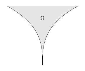
Figure 1: Example of a (non-Sobolev-extension) domain $\Omega$ satisfying 4.1

Remark 4.4.

In the case $V=W^{1,2}(\Omega)$, so the largest of the form domains considered in this work, 4.1 is exhaustively discussed in [25, Section 6.3.4]. See Figure 1 for the exemplary, two dimensional domain $\Omega=\{x\in\mathbb{R}^{2}\colon 0<x_{2}<1,\,|x_{1}|\leq x_{2}^{3}\}$ which satisfies 4.1 for $\beta\leq 4$ ([24]). As visible there, such a domain $\Omega$ may have outward cusps, hence it need be neither a $d$-set (see (9) below) nor a homogeneous space (see [10, Section 2]). Therefore $\Omega$ will in general not admit a continuous linear extension operator $E\colon W^{1,2}(\Omega)\to W^{1,2}(\mathbb{R}^{d})$ such that $(Eu)_{|\Omega}=u$ ([17]). There may however be an continuous linear extension operator $V\to W^{1,2}(\mathbb{R}^{d})$, see e.g. [14, Sect. 6]. The existence of either extension operator would imply the optimal $\beta$ in 4.1. Note moreover that there might exist bounded extension operators $W^{1,2}(\Omega)\to W^{1,r}(\mathbb{R}^{d})$ for $r<2$ or even $W^{1,2}(\Omega)\to W^{\alpha,2}(\mathbb{R}^{d})$ for $\alpha<1$ for domains satisfying 4.1. Conversely, for $r$ or $\alpha$ sufficiently large, the existence such an extension operator would imply 4.1. We refer to [33] and the references therein.

5 An extension to Robin and dynamical boundary conditions

We next show how the generality of the foregoing results, in particular Theorem 3.3, can be used to obtain uniform resolvent estimates for differential operators attached to more sophisticated problems. To this end, we need some regularity assumption on $\Omega$ and the boundary part $D$ in order to have a well defined trace-type operator. We assume that $\Omega$ is bounded throughout this section. The regularity assumption is as follows.

Assumption 5.1.

1. For every point $x\in\Gamma\coloneqq\overline{\partial\Omega\setminus D}$, there is an open neighbourhood $U_{x}$ of $x$ such that $U_{x}\cap\Omega$ is connected and there exists a continuous linear extension operator $E\colon W^{1,2}(U_{x}\cap\Omega)\to W^{1,2}(\mathbb{R}^{d})$; that is, $(Eu)_{|U_{x}\cap\Omega}=u$ for every $u\in W^{1,2}(U_{x}\cap\Omega)$.

2. The set $\Gamma$ is a $(d-1)$-set.

Recall that a Borel set $E\subset\mathbb{R}^{d}$ is an $N$-set or $N$-regular if there exists a constant $c>0$ such that

$$cr^{N}\leq\mathcal{H}_{N}\bigl{(}E\cap B_{r}(x)\bigr{)}\leq c^{-1}r^{N}\quad(x\in E,~{}r\leq 1)$$ (9)

where $\mathcal{H}_{N}$ denotes the $N$-dimensional Hausdorff measure. We refer to [18, Ch. II.1] for more details.

Remark 5.2.

The regularity assumption on $\Gamma=\overline{\partial\Omega\setminus D}$ in 5.1 is very mild. The required Sobolev extension property is a deeply researched subject. Note that while there $D$ need only be closed, there is a condition on the the relative boundary $\partial D$ of $D$ within $\partial\Omega$, so the transition region between Dirichlet and Neumann boundary parts. Particular cases in which 5.1 is satisfied include the one where there are Lipschitz charts available around $\Gamma$, or, more generally, when $\Omega$ is locally an $(\varepsilon,\delta)$-domain around $\Gamma$. The latter is in fact optimal for $d=2$. We refer to [14, Section 6.4] for more information.

The immediate consequences of 5.1 needed in the following are as follows:

1. There is a bounded linear extension operator which extends both $\widetilde{W^{1,2}_{D}(\Omega)}$ and $W^{1,2}_{D}(\Omega)$ to $W^{1,2}_{D}(\mathbb{R}^{d})$ ([14, Theorem 6.9]). In particular, these spaces coincide.

2. There is a well defined trace map $\operatorname{tr}\colon W^{1,2}_{D}(\Omega)\to L^{\beta}(\Gamma;\mathcal{H}_{d-1})$, where $\beta>2$ ([3]).

Hence, for nonnegative $b\in L^{\infty}(\Gamma;\mathcal{H}_{d-1})$, the form $\mathfrak{b}\colon V\times V\to\mathbb{C}$ given by

$$\mathfrak{b}(u,v)\coloneqq\mathfrak{a}(u,v)+\int_{\Gamma}b\,(\operatorname{tr}u)(\overline{\operatorname{tr}v})\;d{\mathcal{H}}_{d-1}\quad(u,v\in V),$$

is well defined, continuous, closed and accretive. In fact, it is even a sub-Markovian form. The operator $B_{2}$ on $L^{2}(\Omega)$ associated with this form is the negative generator of an analytic contraction semigroup $S_{2}$ which extends consistently to contraction semigroups $S_{p}$ on all $L^{p}(\Omega)$-spaces, $p\in[1,\infty[$. The negative generator of $S_{p}$ is denoted by $B_{p}$. All these properties follow as in Section 2.

The operators $B_{p}$ are realizations of the second order elliptic operator $-\operatorname{div}(a\,\nabla\cdot)$ with mixed Dirichlet and Robin boundary conditions. The corresponding parabolic evolution problem associated with $B_{p}$ is formally

$$u_{t}-\operatorname{div}(a\,\nabla u) =f \text{in }(0,\infty)\times\Omega,$$

$$u =0 \text{on }(0,\infty)\times D,$$

$$\langle a\nabla u,\nu\rangle+bu =0 \text{on }(0,\infty)\times(\partial\Omega\setminus D),$$

$$u(0,\cdot) =u_{0} \text{in }\Omega,$$

where $\nu$ is the unit outer normal. That is, one has Dirichlet boundary conditions on $D$ and Robin boundary conditions on $\partial\Omega\setminus D$, which reduce to Neumann boundary conditions on the set $[b=0]$.

Since

$$\int_{\Gamma}b\,(\operatorname{tr}u)(\operatorname{tr}|u|^{p-2}\bar{u})\;d{\mathcal{H}}_{d-1}=\int_{\Gamma}b\operatorname{tr}(|u|^{p})\;d{\mathcal{H}}_{d-1}\geq 0$$

for every $u\in V\cap L^{\infty}(\Omega)$, by Theorem 3.3, the numerical range of the operator $B_{p}$ is contained in the same sector as the numerical range of the operator $A_{p}$. From Theorem 3.5 and the proof of Corollary 3.8, we thus obtain the following result. (Ultracontractivity is inferred from the $W^{1,2}$-extension property of $V$, see Remark 4.4, and Proposition 4.2.)

Theorem 5.3.

For every $p\in[2,\infty[$, the numerical range of $B_{p}$ is contained in the sector $\overline{\Sigma_{\theta_{p}}}$, where $\theta_{p}$ is as in Theorem 3.5. Moreover, for every $p\in\mathopen{]}1,\infty[$,

$$\bigl{\|}(z-B_{p})^{-1}\bigr{\|}_{\mathcal{L}(L^{p}(\Omega))}\leq\frac{1}{\operatorname{dist}(z,\Sigma_{\theta_{p}})}$$ (10)

for every $z\in\mathbb{C}\setminus\overline{\Sigma_{\theta_{p}}}$ and the semigroup generated by $-B_{p}$ extends to an analytic contraction semigroup on the sector $\Sigma_{\frac{\pi}{2}-\theta_{p}}$ and is ultracontractive.

It is also possible to treat dynamical boundary conditions in this approach. Fix a measurable subset $S\subseteq\Gamma$. Then the embedding $j\colon V\to L^{2}(\Omega)\times L^{2}(S;\mathcal{H}_{d-1})$ defined by $u\mapsto(u,\operatorname{tr}u)$ is continuous, injective and has dense range, see [31, Lemma 2.10]. Via this embedding, the form $(\mathfrak{b},V)$ induces also an operator $\hat{B}_{2}$ on the Hilbert space $H=L^{2}(\Omega)\times L^{2}(S;\mathcal{H}_{d-1})$. By [31, Proposition 2.16], the form $\mathfrak{b}$ is sub-Markovian, so that $-\hat{B}_{2}$ generates an analytic contraction semigroup $\hat{S}_{2}$ which extends consistently to contraction semigroups $\hat{S}_{p}$ on all $L^{p}(\Omega)\times L^{p}(S;\mathcal{H}_{d-1})$-spaces, $p\in[1,\infty[$. The negative generator of $\hat{S}_{p}$ is denoted by $\hat{B}_{p}$.

The corresponding parabolic evolution problem associated with $\hat{B}_{p}$ is formally

$$u_{t}-\operatorname{div}(a\,\nabla u) =f \text{in }(0,\infty)\times\Omega,$$

$$u =0 \text{on }(0,\infty)\times D,$$

$$u_{t}+\langle a\nabla u,\nu\rangle+bu =g \text{on }(0,\infty)\times S,$$

$$\langle a\nabla u,\nu\rangle+bu =0 \text{on }(0,\infty)\times(\partial\Omega\setminus(D\cup S)),$$

$$u(0,\cdot) =u_{0} \text{in }\Omega,$$

that is, one has Dirichlet boundary conditions on $D$, dynamical boundary conditions on $S$, and Robin boundary conditions on $\partial\Omega\setminus(D\cup S)$, which reduce to Neumann boundary conditions on the set $[b=0]$. Since $\hat{B}_{p}$ is again fundamentally linked to the form $\mathfrak{a}$, the result about the numerical range transfers immediately from Theorem 3.3. Regarding ultracontractivity, we refer to continuity of the trace operator $\operatorname{tr}\colon V\to L^{\beta}(S;\mathcal{H}_{d-1})$ where $\beta>2$ and the reasoning in [31, Lemma 2.19].

Theorem 5.4.

For every $p\in[2,\infty[$, the numerical range of $\hat{B}_{p}$ is contained in the sector $\overline{\Sigma_{\theta_{p}}}$, where $\theta_{p}$ is as in Theorem 3.5. Moreover, for every $p\in\mathopen{]}1,\infty[$,

$$\bigl{\|}(z-\hat{B}_{p})^{-1}\bigr{\|}_{\mathcal{L}(L^{p}(\Omega))}\leq\frac{1}{\operatorname{dist}(z,\Sigma_{\theta_{p}})}$$ (11)

for every $z\in\mathbb{C}\setminus\overline{\Sigma_{\theta_{p}}}$ and the semigroup generated by $-\hat{B}_{p}$ extends to an analytic contraction semigroup on the sector $\Sigma_{\frac{\pi}{2}-\theta_{p}}$ and is ultracontractive.

Remark 5.5.

It would also be possible to include a $(d-1)$-regular hyperplane $\Sigma\subset\Omega$ in $S$ in a straightforward manner. This would then lead to a dynamic “jump condition”

$$u_{t}+\bigl{[}\langle\mathfrak{a}\nabla u,\nu_{\Sigma}\rangle\bigr{]}=h\quad\text{on}~{}(0,\infty)\times\Sigma.$$

We refer to [31].

6 Appendix: Intrinsic characterization for the form domain

In this section, we give a completely intrinsic characterization for $V=W^{1,2}_{D}(\Omega)$, corresponding to the philosophy in [32], see especially Remark 4 there. In fact, we do so for the full scale $W^{1,p}_{D}(\Omega)$ with $p\in\mathopen{]}1,\infty[$. We suppose that $\Omega$ is bounded and let $p\in\mathopen{]}1,\infty[$ be fixed throughout this section. The characterization is given under following very mild assumption on $\partial\Omega$ and $D$ which we assume to hold for the rest of this appendix:

Assumption 6.1.

1. For every point $x\in\partial D$, the relative boundary of $D$ within $\partial\Omega$, there is an open neighbourhood $U_{x}$ of $x$ such that $U_{x}\cap\Omega$ is connected and there exists a continuous linear extension operator $E\colon W^{1,p}(U_{x}\cap\Omega)\to W^{1,p}(\mathbb{R}^{d})$; that is, $(Eu)_{|U_{x}\cap\Omega}=u$ for all $u\in W^{1,p}(U_{x}\cap\Omega)$.

2. The boundary $\partial\Omega$ and the set $D$ itself are $(d-1)$-sets.

Remark 6.2.

Comparing to 5.1—which we do not suppose to hold for this section—, the Sobolev extension condition is required only on the relative boundary $\partial D$ of $D$ within $\partial\Omega$. Thus, the remaining part of $\partial\Omega\setminus\partial D$ might be highly irregular in a topological sense. We do however suppose the measure-theoretic condition that $\partial\Omega$ and $D$ are $(d-1)$-regular in 6.1, which is not included in 5.1 and which effectively means that $\Gamma=\partial\Omega\setminus D$ is also $(d-1)$-regular.

For closed $E\subseteq\partial\Omega$, we define the spaces

$$\underline{W}^{1,p}_{E}(\Omega)\coloneqq\bigl{\{}u\in W^{1,p}(\Omega)\colon\operatorname{dist}(\operatorname{supp}u,E)>0\bigr{\}},$$

and

$$C^{\infty}_{E}(\Omega)\coloneqq\bigl{\{}u\in C^{\infty}(\Omega)\colon u=v|_{\Omega}~{}\text{for}~{}v\in C^{\infty}_{c}(\mathbb{R}^{d}),\,\operatorname{supp}v\cap E=\emptyset\bigr{\}},$$

and their closures in $W^{1,p}(\Omega)$:

$$W^{1,p}_{E}(\Omega)\coloneqq\overline{\underline{W}^{1,p}_{E}(\Omega)}^{W^{1,p}(\Omega)}\text{ and }\widetilde{W^{1,p}_{E}(\Omega)}\coloneqq\overline{C^{\infty}_{E}(\Omega)}^{W^{1,p}}.$$

We have already seen the latter two spaces in the previous sections in the special case $p=2$. The characterization of $W^{1,p}_{D}(\Omega)$ is as follows. (We use $\operatorname{dist}_{D}(x)\coloneqq\operatorname{dist}(x,D)$.)

Theorem 6.3.

Let $u\in W^{1,p}(\Omega)$. The following are equivalent.

1. $u\in W^{1,p}_{D}(\Omega)$.

2. $u/\operatorname{dist}_{D}\in L^{p}(\Omega)$.

3. For $\mathcal{H}_{d-1}$-almost every $x\in D$,

   $$\lim_{r\searrow 0}\frac{1}{|B_{r}(x)|}\int_{B_{r}(x)\cap\Omega}|u|=0.$$

Remark 6.4.

If one and thus all of the conditions in Theorem 6.3 hold true, then we have a Hardy inequality for elements of $W^{1,p}_{D}(\Omega)$:

$$\left(\int_{\Omega}\left|\frac{u}{\operatorname{dist}_{D}}\right|^{p}\right)^{\frac{1}{p}}\lesssim\|u\|_{W^{1,p}(\Omega)}\quad(u\in W^{1,p}_{D}(\Omega)).$$

In particular,

$$u\mapsto\|u\|_{W^{1,p}(\Omega)}+\left\|\frac{u}{\operatorname{dist}_{D}}\right\|_{L^{p}(\Omega)}$$

is an equivalent norm on $W^{1,p}_{D}(\Omega)$.

A consequence of the characterization of $W^{1,p}_{D}(\Omega)$ in Theorem 6.3 is that the constant one function $\mathbf{1}$ is not an element of that space if $D\neq\emptyset$. The proof follows after the one of Theorem 6.3 below.

Corollary 6.5.

Let $\mathbf{1}\in W^{1,p}(\Omega)$ denote the constant one function. If $D\neq\emptyset$, then $\mathbf{1}\notin W^{1,p}_{D}(\Omega)$.

We next prove a preliminary geometric lemma which will allow us to prove Theorem 6.3 by reducing it to a similar characterization theorem in a more regular situation, Proposition 6.8 below. It says that a subset of a regular set can be extended to a regular set in an arbitrarily small manner. We state and prove it for a general bounded $N$-regular set $\Lambda$. The proof relies on a sort of dyadic decomposition for regular sets established by David and refined by Christ and is given at the very end of the paper.

Lemma 6.6.

Let $\Lambda\subset\mathbb{R}^{d}$ be bounded and $N$-regular. Let further $\Xi\subseteq\Lambda$ and $\rho>0$. Then there exists an $N$-set $\Xi^{\bullet}$ such that $\Xi\subseteq\Xi^{\bullet}\subseteq\Lambda$ and $\sup\{\operatorname{dist}(x,\Xi)\colon x\in\Xi^{\bullet}\setminus\Xi\}\leq\rho$.

Corollary 6.7.

There exists a closed $(d-1)$-set $\Upsilon\subseteq\partial\Omega$ such that $\operatorname{dist}(\Upsilon,D)>0$ and for every point $x\in\overline{\partial\Omega\setminus(D\cup\Upsilon)}$ there is an open neighbourhood $U_{x}$ of $x$ such that $U_{x}\cap\Omega$ is connected and there exists a continuous linear extension operator $E\colon W^{1,p}(U_{x}\cap\Omega)\to W^{1,p}(\mathbb{R}^{d})$.

Proof.

By 6.1, for every $x\in\partial D$ there exists an open $W^{1,p}$-extension neighbourhood $U_{x}$ of $x$. The family $(U_{x})_{x\in\partial D}$ is then an open covering of $\partial D$. By compactness, it thus admits a finite subcovering $(U_{x_{j}})_{j}$.

Now choose $\varepsilon>0$ such that $\{x\in\mathbb{R}^{d}\colon\operatorname{dist}(x,\partial D)<3\varepsilon\}\subseteq\bigcup_{j}U_{x_{j}}$, and set $C\coloneqq\{x\in\partial\Omega\setminus D\colon\operatorname{dist}(x,\partial D)\geq 2\varepsilon\}$. Clearly, for every $x\in\partial\Omega\setminus\overline{(D\cup C)}$ there is an open $W^{1,p}$-extension neighbourhood. Let $C^{\bullet}$ be a $(d-1)$ regular set containing $C$ with $\sup\{\operatorname{dist}(x,C)\colon x\in C^{\bullet}\setminus C\}\leq\varepsilon$ and define $\Upsilon\coloneqq\overline{C^{\bullet}}$; such a set exists by Lemma 6.6. Then $\Upsilon$ has the required properties; for the $(d-1)$ property, see [18, Ch. VIII Proposition 1]. ∎

With the foregoing result, we can now make use of the characterisation of a zero trace property for a more regular situation in [15] which we quote adapted to our setting:

Proposition 6.8 ([15, Theorem 2.1]).

Let $\Upsilon\subseteq\partial\Omega$ be a closed $(d-1)$-set such that for every point $x\in\overline{\partial\Omega\setminus(D\cup\Upsilon)}$ there is an open neighbourhood $U_{x}$ of $x$ such that $U_{x}\cap\Omega$ is connected and there exists a continuous linear extension operator $E\colon W^{1,p}(U_{x}\cap\Omega)\to W^{1,p}(\mathbb{R}^{d})$. Let $u\in W^{1,p}(\Omega)$. Then the following are equivalent:

1. $u\in\widetilde{W^{1,p}_{D\cup\Upsilon}(\Omega)}$.

2. $u/\operatorname{dist}_{D\cup\Upsilon}\in L^{p}(\Omega)$.

3. For $\mathcal{H}_{d-1}$-a.e. $x\in D\cup\Upsilon$,

   $$\lim_{r\searrow 0}\frac{1}{|B_{r}(x)|}\int_{B_{r}(x)\cap\Omega}|u|=0.$$

Proof of Theorem 6.3.

Choose $\Upsilon\subseteq\partial\Omega$ as in Corollary 6.7 and a cut-off function $\eta\in C^{\infty}_{c}(\mathbb{R}^{d})$ such that $\operatorname{supp}\eta\cap\Upsilon=\emptyset$ and $\eta=1$ in a neighbourhood of $D$. Write $u=(1-\eta)u+\eta u$. Clearly, $(1-\eta)u\in\underline{W}^{1,p}_{D}(\Omega)$, so $(1-\eta)u/\operatorname{dist}_{D}\in L^{p}(\Omega)$ and

$$\lim_{r\searrow 0}\frac{1}{|B_{r}(x)|}\int_{B_{r}(x)\cap\Omega}|(1-\eta)u|=0.$$

It is thus sufficient to prove all equivalences for $\eta u$ only.

(i $\implies$ ii): Let $\eta u\in W^{1,p}_{D}(\Omega)$. Choose a sequence $(u_{k})\subset\underline{W}^{1,p}_{D}(\Omega)$ approximating $u$ in $W^{1,p}(\Omega)$. We have $\eta u_{k}/\operatorname{dist}_{D\cup\Upsilon}\in L^{p}(\Omega)$ and $\eta u_{k}\to\eta u$ in $W^{1,p}(\Omega)$. Proposition 6.8 implies that the set of $v\in W^{1,p}(\Omega)$ satisfying $v/\operatorname{dist}_{D\cup\Upsilon}\in L^{p}(\Omega)$ is closed in $W^{1,p}(\Omega)$. Hence $\eta u/\operatorname{dist}_{D}\in L^{p}(\Omega)$.

(ii $\implies$ i): Let $\eta u/\operatorname{dist}_{D}\in L^{p}(\Omega)$. Then $\eta u/\operatorname{dist}_{D\cup\Upsilon}\in L^{p}(\Omega)$ and $\eta u\in\widetilde{W^{1,p}_{D\cup\Upsilon}(\Omega)}$ by Proposition 6.8. In particular, $\eta u$ in $W^{1,p}(\Omega)$ can be approximated by a sequence of functions from $C_{D\cup\Upsilon}^{\infty}(\Omega)$. But $C_{D\cup\Upsilon}^{\infty}(\Omega)\subset\underline{W}^{1,p}_{D}(\Omega)$, so $\eta u\in W^{1,p}(\Omega)$.

(ii $\iff$ iii): Apply Proposition 6.8 to $\eta u$. ∎

Proof of Corollary 6.5.

Suppose that $\mathbf{1}\in W^{1,p}_{D}(\Omega)$. Then, by Theorem 6.3,

$$\lim_{r\searrow 0}\frac{1}{|B(y,r)|}\int_{B(r,y)\cap\Omega}\mathbf{1}=\lim_{r\searrow 0}\frac{|B(y,r)\cap\Omega|}{|B(y,r)|}=0$$ (12)

for $\mathcal{H}_{d-1}$-almost every $y\in D$. We will show that this leads to a contradiction.

Let $x\in\partial D$, the relative boundary of $D$ within $\partial\Omega$. By 6.1, there exists an open neighbourhood $U_{x}$ of $x$ such that $U_{x}\cap\Omega$ has the $W^{1,p}$-extension property. A domain with the $W^{1,p}$-extension property is necessarily $d$-regular by a fundamental result by Hajłasz, Koskela and Tuominen [17], so there is a constant $c>0$ such that

$$|B(y,r)\cap\Omega\cap U_{x}|\geq cr^{d}\quad(y\in\Omega\cap U_{x},~{}r\leq 1).$$

This property also holds for $y\in\partial\Omega\cap U_{x}\subset\partial(\Omega\cap U_{x})$. Indeed, let $r\leq 1$ and choose $z\in B(y,r/2)\cap\Omega\cap U_{x}$. Then $B(z,r/2)\cap\Omega\cap U_{x}\subset B(y,r)\cap\Omega\cap U_{x}$, hence

$$|B(y,r)\cap\Omega\cap U_{x}|\geq c2^{-d}r^{d}\quad(y\in\partial\Omega\cap U_{x},~{}r\leq 1).$$ (13)

Now let $0<r_{0}\leq 1$ be such that $B(x,2r_{0})\subset U_{x}$. Consider $y\in B(x,r_{0})\cap D$. Then $B(y,r_{0})\subset U_{x}$, so there is a constant $c_{0}>0$ such that

$$\frac{|B(y,r)\cap\Omega|}{|B(y,r)|}=\frac{|B(y,r)\cap\Omega\cap U_{x}|}{|B(y,r)|}\geq c_{0}>0$$

for all $r\leq r_{0}$ by (13). By (12), this is only possible if $\mathcal{H}_{d-1}(B(x,r_{0})\cap D)=0$. But $D$ is $(d-1)$-regular, so $\mathcal{H}_{d-1}(B(x,r_{0})\cap D)>0$. This is the contradiction. ∎

Proof of Lemma 6.6

In this final subsection, we prove Lemma 6.6. As already mentioned above, the proof relies on the following Christ decomposition for regular sets:

Theorem 6.9 ([8, Theorem 11]).

Let $\Lambda\subset\mathbb{R}^{d}$ be bounded and $N$-regular. Then there exists a collection of open sets $\{Q_{\alpha}^{k}\subseteq\Lambda\colon k\in\mathbb{N}_{0},~{}\alpha\in I_{k}\}$, where $I_{k}$ is an index set for every $k\in\mathbb{N}_{0}$, and constants $\delta\in\mathopen{]}0,1[$, $a_{0}>0$, $c_{1}<\infty$ such that the following hold true:

1. $\mathcal{H}_{N}\bigl{(}\Lambda\setminus\bigcup_{\alpha\in I_{k}}Q_{\alpha}^{k}\bigr{)}=0$ for every $k\in\mathbb{N}_{0}$,

2. if $\ell,k\in\mathbb{N}_{0}$ and $\ell\geq k$, then for every $\alpha\in I_{k}$ and $\beta\in I_{\ell}$, either $Q_{\beta}^{\ell}\cap Q_{\alpha}^{k}=\emptyset$ or $Q_{\beta}^{\ell}\subseteq Q_{\alpha}^{k}$,

3. if $k\in\mathbb{N}_{0}$ and $\alpha,\beta\in I_{k}$, then $Q_{\beta}^{k}\cap Q_{\alpha}^{k}=\emptyset$,

4. for every $k\in\mathbb{N}_{0}$ and $\alpha\in I_{k}$, there holds $\operatorname{diam}(Q_{\alpha}^{k})\leq c_{1}\delta^{k}$,

5. for every $k\in\mathbb{N}_{0}$ and $\alpha\in I_{k}$, there is $z_{\alpha}^{k}\in\Lambda$ such that $B(z_{\alpha}^{k},a_{0}\delta^{k})\cap\Lambda\subseteq Q_{\alpha}^{k}$.

Remark 6.10.

It will be useful to observe that by property v of the Christ decomposition in Theorem 6.9 and $N$-regularity of $\Lambda$, there is a constant $c>0$ such that

$$\mathcal{H}_{N}(Q_{\alpha}^{k})\geq\mathcal{H}_{N}\bigl{(}B(z_{\alpha}^{k},a_{0}\delta^{k})\cap\Lambda\bigr{)}\geq c(a_{0}\delta^{k})^{N}\quad(\alpha\in I_{k})$$ (14)

for all $k\in\mathbb{N}_{0}$ such that $a_{0}\delta^{k}\leq 1$.

In fact, the Christ decomposition as established in [8, Theorem 11] has some more properties and is valid for locally doubling metric measure spaces in general; the “locally” part is due to Morris [26, Proposition 4.2]. We have just extracted the necessary bits needed to prove Lemma 6.6 which we repeat:

Let $\Lambda\subset\mathbb{R}^{d}$ be bounded and $N$-regular. Let further $\Xi\subseteq\Lambda$ and $\rho>0$. Then there exists an $N$-set $\Xi^{\bullet}$ such that $\Xi\subseteq\Xi^{\bullet}\subseteq\Lambda$ and $\sup\{\operatorname{dist}(x,\Xi)\colon x\in\Xi^{\bullet}\setminus\Xi\}\leq\rho$.

Proof of Lemma 6.6.

Consider the Christ decomposition of $\Lambda$ and its data as stated in Theorem 6.9. Let $M\in\mathbb{N}_{0}$ be so large that $c_{1}\delta^{M}\leq\rho\wedge 1$ and define

$$\Xi^{\bullet}\coloneqq\Xi\cup\bigl{\{}Q_{\alpha}^{M}\colon\alpha\in I_{M},~{}Q_{\alpha}^{M}\cap\Xi\neq\emptyset\bigr{\}}.$$

By the choice of $M$ and property iv of the Christ decomposition, we already have $\sup\{\operatorname{dist}(x,\Xi)\colon x\in\Xi^{\bullet}\setminus\Xi\}\leq\rho$. We show that $\Xi^{\bullet}$ is $N$-regular. Since $\Xi^{\bullet}\subseteq\Lambda$ and the latter is $N$-regular, the upper estimate $\mathcal{H}_{N}(\Xi^{\bullet}\cap B(x,r))\lesssim r^{N}$ for all $x\in\Xi^{\bullet}$ and $r\leq 1$ as in (9) is for free.

For the lower estimate, let $x\in\Xi^{\bullet}$. If there is $\alpha\in I_{M}$ such that $x\in Q_{\alpha}^{M}$, then $Q_{\alpha}^{M}\subseteq\Xi^{\bullet}$ due to property iii of the Christ decomposition. Thus it is enough to show the lower estimate for $N$-regularity for $Q_{\alpha}^{M}$. (Of course, we thereby prove that $Q_{\alpha}^{M}$ is $N$-regular since the upper estimate is again for free.)

In fact, we can assume even that $x$ is an element of a member of every generation $k\in\mathbb{N}_{0}$, i.e.,

$$x\in\Upsilon\coloneqq\bigl{\{}y\in\Lambda\colon\text{for every}~{}k\in\mathbb{N}_{0}~{}\text{there is}~{}\alpha\in I_{k}~{}\text{such that}~{}y\in Q_{\alpha}^{k}\bigr{\}}.$$

Indeed, suppose we want to show a lower $N$-regularity estimate for $z\in\Lambda\setminus\Upsilon$. The set $\Lambda\setminus\Upsilon$ is of $\mathcal{H}_{N}$-measure zero by property i of the Christ decomposition. For every $r\leq 1$, the intersections $\Lambda\cap B(z,r/2)$ have positive $\mathcal{H}_{N}$-measure by $N$-regularity of $\Lambda$, hence they cannot be subsets of $\Lambda\setminus\Upsilon$. This implies that for every $r\leq 1$, there is $x\in\Upsilon\cap B(z,r/2)$. Since $B(z,r)$ contains $B(x,r/2)$, it is thus enough to prove the lower estimate for $N$-regularity for $x\in\Upsilon$.

So, let $x\in\Upsilon$ and let $\alpha\in I_{M}$ be such that $x\in Q_{\alpha}^{M}$.

First suppose that $c_{1}\delta^{M}<r\leq 1$. Then, by property iv of the Christ decomposition, $Q_{\alpha}^{M}\cap B(x,r)=Q_{\alpha}^{M}$. So, using (14),

$$\mathcal{H}_{N}\bigl{(}Q_{\alpha}^{M}\cap B(x,r)\bigr{)}=\mathcal{H}_{N}(Q_{\alpha}^{M})\geq c(a_{0}\delta^{M})^{N}\geq c(a_{0}\delta^{M})^{N}r^{N}.$$

Next, let $r\leq c_{1}\delta^{M}$. Choose $\ell\in\mathbb{N}_{0}$ such that $c_{1}\delta^{\ell}\leq r\leq c_{1}\delta^{\ell-1}$. Clearly, $\ell>M$. Due to $x\in\Upsilon$, there exists $\beta\in I_{\ell}$ such that $x\in Q_{\beta}^{\ell}$ and we have $Q_{\beta}^{\ell}\subseteq Q_{\alpha}^{M}$ by property ii of the Christ decomposition. Again, from property iv of the Christ decomposition and the choice of $\ell$ we have $Q_{\beta}^{\ell}\cap B(x,r)=Q_{\beta}^{\ell}$. Using (14) and the choice of $\ell$,

$$\mathcal{H}_{N}\bigl{(}Q_{\alpha}^{M}\cap B(x,r)\bigr{)} \geq\mathcal{H}_{N}\bigl{(}Q_{\beta}^{\ell}\cap B(x,r)\bigr{)}=\mathcal{H}_{N}(Q_{\beta}^{\ell})$$

$$\geq c(a_{0}\delta^{\ell})^{N}\geq c(a_{0}\delta/c_{1})^{N}r^{N}.$$

This completes the proof. ∎

Acknowledgment. We wish to thank Pertti Mattila (University of Helsinki) and Moritz Egert (Université Paris-Sud) for pointing out the Christ decomposition and ideas for the proof of Lemma 6.6.

References

- [1] Herbert Amann, Linear and quasilinear parabolic problems. Vol. I, Monographs in Mathematics, vol. 89, Birkhäuser Boston, Inc., Boston, MA, 1995, Abstract linear theory.
- [2] W. Arendt, Semigroups and evolution equations: functional calculus, regularity and kernel estimates, Handbook of Differential Equations (C. M. Dafermos, E. Feireisl eds.), Elsevier/North Holland, 2004, pp. 1–85.
- [3] Markus Biegert, On traces of Sobolev functions on the boundary of extension domains, Proc. Amer. Math. Soc. 137 (2009), no. 12, 4169–4176.
- [4] Kevin Brewster, Dorina Mitrea, Irina Mitrea, and Marius Mitrea, Extending Sobolev functions with partially vanishing traces from locally -domains and applications to mixed boundary problems, J. Funct. Anal. 266 (2014), no. 7, 4314–4421.
- [5] Andrea Carbonaro and Oliver Dragičević, Convexity of power functions and bilinear embedding for divergence-form operators with complex coefficients, J. Eur. Math. Soc. (2019), no. to appear.
- [6] R. Chill, E. Fašangová, G. Metafune, and D. Pallara, The sector of analyticity of the Ornstein-Uhlenbeck semigroup in spaces with respect to invariant measure, J. London Math. Soc. 71 (2005), 703–722.
- [7] , The sector of analyticity of nonsymmetric submarkovian semigroups generated by elliptic operators, C. R. Acad. Sci. Paris 342 (2006), 909–914.
- [8] Michael Christ, A theorem with remarks on analytic capacity and the cauchy integral, Colloquium Mathematicae 60-61 (1990), no. 2, 601–628 (eng).
- [9] A. Cialdea and V. Maz’ya, Criterion for the -dissipativity of second order differential operators with complex coefficients, J. Math. Pures Appl. (9) 84 (2005), no. 8, 1067–1100.
- [10] Ronald R. Coifman and Guido Weiss, Extensions of Hardy spaces and their use in analysis, Bull. Amer. Math. Soc. 83 (1977), no. 4, 569–645.
- [11] D. Daners, A priori estimates for solutions to elliptic equations on non-smooth domains, Proc. Roy. Soc. Edinburgh Sect. A 132 (2002), 793–813.
- [12] E. B. Davies, Heat kernels and spectral theory, Cambridge Tracts in Mathematics, vol. 92, Cambridge University Press, Cambridge, 1989.
- [13] R. Denk, M. Hieber, and J. Prüss, -Boundedness, Fourier Multipliers and Problems of Elliptic and Parabolic Type, Memoirs Amer. Math. Soc., vol. 166, Amer. Math. Soc., Providence, R.I., 2003.
- [14] Moritz Egert, Robert Haller-Dintelmann, and Joachim Rehberg, Hardy’s inequality for functions vanishing on a part of the boundary, Potential Anal. 43 (2015), no. 1, 49–78.
- [15] Moritz Egert and Patrick Tolksdorf, Characterizations of Sobolev functions that vanish on a part of the boundary, Discrete Contin. Dyn. Syst. Ser. S 10 (2017), no. 4, 729–743.
- [16] J. A. Griepentrog, H.-C. Kaiser, and J. Rehberg, Heat kernel and resolvent properties for second order elliptic differential operators with general boundary conditions on , Adv. Math. Sci. Appl. 11 (2001), no. 1, 87–112.
- [17] Piotr Hajłasz, Pekka Koskela, and Heli Tuominen, Sobolev embeddings, extensions and measure density condition, J. Funct. Anal. 254 (2008), no. 5, 1217–1234.
- [18] Alf Jonsson and Hans Wallin, Function spaces on subsets of , Math. Rep. 2 (1984), no. 1, xiv+221.
- [19] N. Kalton and L. Weis, The -calculus and sums of closed operators, Math. Ann. 321 (2001), 319–345.
- [20] P. C. Kunstmann, -spectral properties of the Neumann Laplacian on horns, comets and stars, Math. Z. 242, 183–201.
- [21] P. C. Kunstmann and L. Weis, Maximal regularity for parabolic equations, Fourier multiplier theorems and functional calculus, Levico Lectures, Proceedings of the Autumn School on Evolution Equations and Semigroups (M. Iannelli, R. Nagel, S. Piazzera eds.), vol. 69, Springer Verlag, Heidelberg, Berlin, 2004, pp. 65–320.
- [22] Damien Lamberton, Équations d’évolution linéaires associées à des semi-groupes de contractions dans les espaces , J. Funct. Anal. 72 (1987), no. 2, 252–262.
- [23] A. Lunardi, Analytic Semigroups and Optimal Regularity in Parabolic Problems, Progress in Nonlinear Differential Equations and Their Applications, vol. 16, Birkhäuser, Basel, 1995.
- [24] V. G. Maz’ya and S. V. Poborchiĭ, Theorems for embedding Sobolev spaces on domains with a peak and on Hölder domains, Algebra i Analiz 18 (2006), no. 4, 95–126.
- [25] Vladimir Maz’ya, Sobolev spaces with applications to elliptic partial differential equations, augmented ed., Grundlehren der Mathematischen Wissenschaften [Fundamental Principles of Mathematical Sciences], vol. 342, Springer, Heidelberg, 2011.
- [26] Andrew J. Morris, The Kato square root problem on submanifolds, Journal of the London Mathematical Society 86 (2012), no. 3, 879–910.
- [27] E. M. Ouhabaz, Analysis of Heat Equations on Domains, London Mathematical Society Monographs, vol. 30, Princeton University Press, Princeton, 2004.
- [28] A. Pazy, Semigroups of Linear Operators and Applications to Partial Differential Equations, Applied Mathematical Sciences, vol. 44, Berlin, 1983.
- [29] Jan Prüss and Gieri Simonett, Moving interfaces and quasilinear parabolic evolution equations, Monographs in Mathematics, vol. 105, Birkhäuser/Springer, [Cham], 2016.
- [30] A. F. M. ter Elst, R. Haller-Dintelmann, J. Rehberg, and P. Tolksdorf, On the -theory for second-order elliptic operators in divergence form with complex coefficients, Preprint (2019), https://arxiv.org/abs/1903.06692.
- [31] A. F. M. ter Elst, M. Meyries, and J. Rehberg, Parabolic equations with dynamical boundary conditions and source terms on interfaces, Ann. Mat. Pura Appl. (4) 193 (2014), no. 5, 1295–1318.
- [32] Hans Triebel, A note on function spaces in rough domains, Tr. Mat. Inst. Steklova 293 (2016), no. Funktsional. Prostranstva, Teor. Priblizh., Smezhnye Razdely Mat. Anal., 346–351, English version published in Proc. Steklov Inst. Math. 293 (2016), no. 1, 338–342.
- [33] Alexander Ukhlov, Extension operators on Sobolev spaces with decreasing integrability, Preprint (2019), https://arxiv.org/abs/1908.09322.