A case–study of multi–temperature coronal jets for emerging flux MHD models

Abstract

Context. Hot coronal jets are a basic observed feature of the solar atmosphere whose physical origin is still being actively debated.

Aims. We study six recurrent jets occurring in the active region NOAA 12644 on April 04, 2017. They are observed in all the hot filters of AIA as well as cool surges in IRIS slit–jaw high spatial and temporal resolution images.

Methods. The AIA filters allow us to study the temperature and the emission measure of the jets using the filter ratio method. We study the pre–jet phases by analysing the intensity oscillations at the base of the jets with the wavelet technique.

Results. A fine co–alignment of the AIA and IRIS data shows that the jets are initiated at the top of a canopy–like, double chambered structure with cool emission in one side and hot emission in the other. The hot jets are collimated in the hot temperature filters, have high velocities (around 250 km s^-1) and accompanied by the cool surges and ejected kernels both moving at about 45 km s^-1. In the pre-phase of the jets, at their base we find quasi-periodic intensity oscillations in phase with small ejections; they have a period between 2 and 6 minutes, and are reminiscent of acoustic or MHD waves.

Conclusions. This series of jets and surges provides a good case–study to test the 2D and 3D magnetohydrodynamic (MHD) models that result from magnetic flux emergence. The double–chambered structure found in the observations corresponds to the cold and hot loop regions found in the models beneath the current sheet that contains the reconnection site. The cool surge with kernels is comparable with the cool ejection and plasmoids that naturally appears in the models.

1 Introduction

Solar coronal jets are detected along the whole solar cycle in a large wavelength range, from X-rays (Shibata et al., 1992) to the EUV (Wang et al., 1998; Alexander & Fletcher, 1999; Innes et al., 2011; Sterling et al., 2015; Chandra et al., 2015; Joshi et al., 2017a). Many are seen as collimated plasma material flowing along open magnetic field lines with high velocity. Other interesting ejections are cool surges, which emerge in the form of unwrinkled threads of dark material in H$\alpha$ (Roy, 1973; Mandrini et al., 2002; Uddin et al., 2012; Li et al., 2016) and sprays, which are very fast ejections having their origin in filaments generally in active regions (Warwick, 1957; Tandberg-Hanssen et al., 1980; Pike & Mason, 2002; Martin, 2015). In fact, some surges are closely related to hot jets (Schmieder et al., 1988; Canfield et al., 1996). Solar coronal jets are observed in active regions (Sterling et al., 2016; Chandra et al., 2017; Joshi & Chandra, 2018) as well as in quiet regions (Hong et al., 2011; Panesar et al., 2016). Their physical parameters such as height (1–50 x 10⁴ km), lifetime (tens of minutes to one hour), width (1–10 x 10⁴ km), and velocity (100–500 km s^-1) have been studied by many authors (Shimojo et al., 1996; Savcheva et al., 2007; Nisticò et al., 2009; Filippov et al., 2009; Joshi et al., 2017b).

Magnetic reconnection is believed to be the triggering mechanism behind the activation of the jet phenomenon according to different theoretical models (Yokoyama & Shibata, 1995; Archontis et al., 2004, 2005; Pariat et al., 2015). Reconnection is a process of restructuring of the magnetic field lines and can occur in 2D (Filippov, 1999; Pontin et al., 2005) or in 3D configurations (Démoulin & Priest, 1993; Filippov, 1999; Longcope et al., 2003; Priest & Pontin, 2009; Masson et al., 2009). In a 2D magnetic null point configuration, magnetic field lines contained in a plane and with opposite orientations come toward each other across an X–point and change connectivity instantaneously; the result are hybrid field lines that are expelled away from the X–point, typically with velocities of order the Alfvén speed. In 3D there is a whole variety of possible patterns (like: spine-fan, torsional, separator reconnection, etc); in many cases the underlying structure is what is known as a fan-spine configuration around a central null point. The field lines from inside the fan surface are joined to open field lines from just outside with ensuing connectivity change. Changes in the remote connectivity of magnetic field lines may also take place in regions with strong spatial gradients of the field components called quasi-separatrix layers (QSLs) (Mandrini et al., 2002).
Magnetic reconnection can take place as a result of a process of magnetic flux emergence from the low solar atmosphere or interior. In typical magnetic flux emergence processes, the emerging magnetized plasma interacts with the pre–existing ambient coronal magnetic field, thus providing a favorable condition for magnetic reconnection, and therefore, for the occurrence of solar jets. The observations indicate that the expansion of the magnetic flux emerging region leads to reconnection with the ambient quasi potential field and magnetic cancellation (Gu et al., 1994; Schmieder et al., 1996; Liu et al., 2011; Guo et al., 2013). A number of numerical models have simulated this process (see, for example Yokoyama & Shibata 1996; Archontis et al. 2004; Moreno-Insertis et al. 2008; Török et al. 2009; Moreno-Insertis & Galsgaard 2013; Archontis & Hood 2013; Nóbrega-Siverio et al. 2016; Ni et al. 2017). In the model by Moreno-Insertis et al. (2008), in particular, a split-vault structure is clearly shown to form below the jet containing two chambers: the chamber containing previously emerged loops with a decrease in volume and the chamber containing reconnected loops with a increase in volume due to reconnection. This structure is also confirmed in radiation–MHD simulations by Nóbrega-Siverio et al. (2016). The observations that motivated those models were either X-ray jets observed by Hinode (Moreno-Insertis et al., 2008), or cool surges observed in chromospheric lines and bright bursts in transition region lines (Nóbrega-Siverio et al., 2017) but these models have not been compared yet with hot jet and cool surges observed simultaneously.
On the other hand, for another category of MHD models the important mechanism which drives the jet onset is not the emerging flux itself but the injection of helicity through photospheric motions (Pariat et al., 2015, 2016); see further references in the review by (Raouafi et al., 2016). The presence of shear and/or twist motions at the base of the closed non potential region under a preexisting null point induces reconnection with the ambient quasi potential flux and initiates untwisting/helical jets (Pariat et al., 2015; Török et al., 2016). In some of these MHD models based on the loss of equilibrium through twisting motions, the thermal plasma parameters of the jets are not directly considered but suggested by correspondence parameters like the plasma $\beta$ (Pariat et al., 2016).

The observational analysis from previous studies has revealed that the jet evolution could be preceded by some wave-like or oscillatory disturbances (Pucci et al., 2012; Li et al., 2015; Bagashvili et al., 2018). Pucci et al. (2012) analysed the X-ray jets observed by Hinode 2007 November 02–04 and found that most of the jets are associated with oscillations of the coronal emission in bright points (for a recent review of coronal bright points, see Madjarska 2019) at the base of the jets. They concluded that the pre–jet oscillations are the result of the change of the area or the temperature of pre–jet activity region. Recently a statistical analysis of pre–jet oscillations of coronal hole jets has been carried out by Bagashvili et al. (2018). They reported that 20 out of 23 jets in their study were preceded by pre–jet intensity oscillations some 12–15 mins before the onset of the jet. They tentatively suggested that these quasi periodic intensity oscillations may be the result of MHD wave generation through rapid temperature variations and shear flows associated with local reconnection events (Shergelashvili et al., 2006).

Here, we found a series of jets observed in the hot EUV channels of SDO/AIA as well as in cool temperatures with IRIS slit–jaw images. The jets were ejected from the active region NOAA 12644 on April 04, 2017; on that date, the region was located at the west limb (N13W91) (Figure 1). When passing through the central meridian, this region had shown high jet activity alongside episodes of emerging magnetic flux (Ruan et al., 2019). Its location at the limb in the present observations allows us to visualize the structure of the brightenings from the side and thus facilitates the comparison with the MHD jet models, which motivates the present research.

The layout of the paper is as follows. We present the observations and kinematics of jets and identify the reconnected structures in section 2. Pre–jet oscillations are reported in section 3. We discuss our results in section 4. We conclude that this series of jet and surge observations obtained with a high spatial and temporal resolution match important aspects of the expected behaviour predicted by the MHD models of emerging flux. We could identify a candidate location for the current sheet and reconnection site and follow the evolution of the cool surge and hot jets with individual blob ejections. This is a clear case-study for the emerging flux MHD jet models.

2 Jets

2.1 Observations

In this study, we select six jet eruptions occurring in the active region NOAA 12644 at the western solar limb on April 04, 2017. We use data from the Atmospheric Imaging Assembly (AIA) (Lemen et al., 2012) on board the Solar Dynamics Observatory (SDO) (Pesnell et al., 2012) and the Interface Region Imaging Spectrograph (IRIS) (De Pontieu et al., 2014). AIA observes the full Sun in seven UV/EUV wavelengths (94 Å, 131 Å, 171 Å, 193 Å, 211 Å, 304 Å, and 335 Å ) with a pixel size and temporal cadence of $0\aas@@fstack{\prime\prime}6$ and 12s, respectively. We align the complete data set using the drot_map routine. For the bad pixel correction, we process the level 1 AIA data to level 1.5 by using the code aia_prep.pro. These codes are available in SolarSoftWare (SSW) in IDL platform. IRIS provides simultaneously spectra and images of the photosphere, chromosphere, transition region, and corona which cover a temperature range between 5000 K to 10 MK. Slit–jaw Images (SJI) are obtained in four different passbands with a high spatial and temporal resolution of $0\aas@@fstack{\prime\prime}16$ pixel^-1 and 1.5 s respectively. The IRIS data set includes two transition region lines (C II 1330 Å, Si IV 1400 Å), one chromospheric line (Mg IIk 2796 Å), and one photospheric passband (in the Mg II wing around 2830 Å). We take the IRIS level 1.5 data from the data archive at http://iris.lmsal.com/search. The level 1.5 data is corrected for dark current and we remove the FUV background data by iris_prep.pro in SSWIDL. The IRIS target was pointed towards the active region NOAA 12644 at the western limb with a field of view of 126$\arcsec$ x 119$\arcsec$ between 11:05:38 UT and 17:58:35 UT. For our current study, we use the SJIs in the C II and Mg II k bandpasses obtained with a cadence of 16s. The SJIs picture the chromospheric plasma around 10⁴ K.

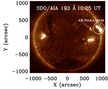
Figure 1: Full disk image of the Sun on April 04, 2017. The solar jets were ejected from the active region NOAA 12644 shown by the white circle at the west limb.

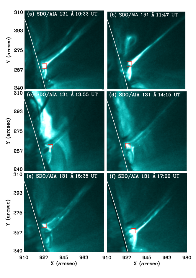
Figure 2: Six solar jets (Jet1–Jet6) in AIA 131 Å filter. The red square in each panel shows the position at which the pre–jet oscillations are measured. The limb is indicated by the white circle part in each panel.

2.2 Characteristics of the jets

On April 04, 2017, active region jets were observed at the limb between 02:30–17:10 UT with AIA. The movies in different wavelengths of AIA (131 Å, 171 Å, and 304 Å) reveal that there are two sites of plasma ejections (jets) along the limb. First, there is a northern site ([921$\arcsec$, 264$\arcsec$]), where the jets are straight and have their base located behind the limb and hence concealed by it. Second, there is a site in the south of the field of view ([931$\arcsec$, 255$\arcsec$]) in which the jets have their base over the limb. Therefore we study in the present paper the six main jets originated in the southern site occurring after 10:00 UT. Five of them were also observed by IRIS, whereas the first of them occurred before the IRIS observations. These jets reach an altitude between 30 and 70 Mm; their recurrence period is around 80 mins, with the exception of two jets which were separated by only 15 min. In the movies we also see many small jets reaching less than 10 Mm height both before and in between the main jets. The jets observed in AIA 131 Å are shown in Figure 2 (a–f) and in an accompanying animation (MOV1). The first main jet, Jet1, reaches its peak at $\approx$ 10:22 UT with an average speed of 210 km s^-1 (panel (a)). Jet2 (panel b) starts at 11:45 UT and reaches its maximum extent at $\approx$ 11:47 UT. In the movie (MOV1) we note a large filament eruption located in the northern site of the jets which erupts $\approx$ 13:30 UT and falls back after reaching its maximum height. Moreover, we could see that the jet and the filament are not associated with each other. Jet3 and Jet4 (panel b and c, respectively) reach their maximum altitude at 13:55 UT and 14:15 UT respectively. Jet5 (panel e) erupts with a broader base and reaches its maximum height at $\approx$ 15:25 UT. We see a fast lateral extension of the jet base along a bright loop. Jet6 (panel f) is ejected at $\approx$ 16:57 UT. A second instance of filament eruption is observed during the peak phase of Jet6 starting again at the same location of the first one. In this case the erupted filament material seems to merge later with the jet material and is ejected in the same direction. However, here the jet is not launched by the filament eruption, because it is not at the jet footpoint.

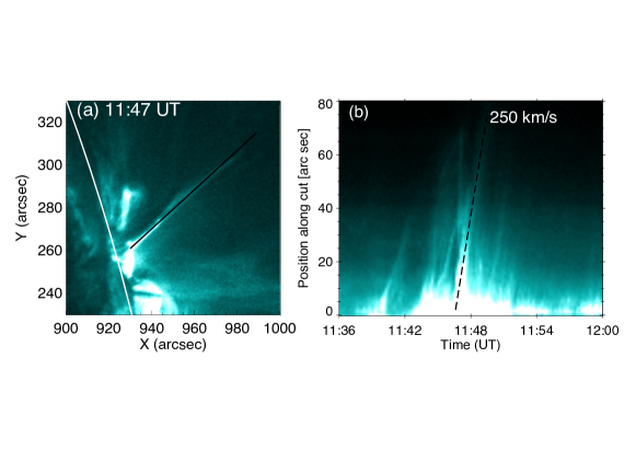
Figure 3: An example of timeslice analysis of the jet 1, used for velocity and height calculations in AIA 131 Å. In panel (a) the solid black line is the slit location, which we use to make the height–time plot (b).

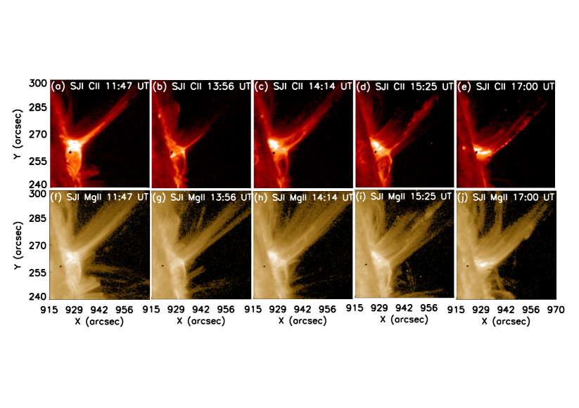
Figure 4: IRIS observed the active region from 11:05 UT to 17:58 UT. It covers five jets in our present analysis in CII (top) and MgII k (bottom) lines. The black points in the top panels are produced by extreme saturation, which we used for a better visibility of jets.

We have computed various physical parameters, namely, height, width, lifetime, speed of these jets using the AIA 131 Å data. For the velocity calculation, we calibrated height–time of each jet in AIA 131 Å fixing a slit in the middle of the jet plasma flow and calculating the average speed in the flow direction. An example of height–time calculation is shown in Figure 3 for Jet2. All computed physical parameters are listed in Table 1. The maximum height, average speed, width, and lifetime of the observed jets vary in the ranges $\approx$ 30–80 Mm, 200–270 km s^-1, 1–7 Mm, and 2–10 min respectively.

Jet2–Jet6 were also observed by IRIS in two wavelength passbands, namely, CII (top row of Figure 4) and MgII k (bottom row). The high spatial resolution of IRIS allowed us to make a clear identification of what looks like a null–point structure at a height of $\approx$ 6 Mm. In the CII filter we see bright loops above a bright half dome in the northern site of the jet footpoints. In the Mg II filter, the northern part of the dome is also bright. We find jet strands all over the northern side of the dome, like a collection of sheets. We will discuss about these jet strands, which are infact cool jets/surges with a lower velocity in section 2.4. In AIA 131 Å we see clearly, for all the jets, a bright area which could correspond to a current sheet (CS), possibly containing a null point, with underlying bright loops shaping a dome (Figure 2). However we notice that the bright dome and loops are located on the southern side of the tentative current sheet, whereas the bright loops in IRIS C II are rather on its northern side. In the following, for simplicity, when referring to observations of this candidate current sheet and possible null point we will sometimes call them ’the null point’ even though there is clearly no way in which one could detect a zero of the magnetic field (nor the intensity of the electric current) in those temperatures with present observational means. Moreover in all the hot channels of AIA (131 Å  193 Å, 171 Å, 211 Å) and IRIS C II and Mg II SJIs the jets have an anemone (“Eiffel–Tower” or “inverted–Y”) structure, with a loop at the base and elongated jet arms (see Figures 2 and 4) as reported in previous events (Nisticò et al., 2009; Schmieder et al., 2013; Liu et al., 2016).

In AIA 131 Å we could also see that between the first and the last jet eruption, the tentative current sheet and the jet spine move towards the south–west direction (Figure 2). More precisely, by following the motion of the point with maximum intensity, we determined a drift of 5 arcsec in less than 6 hours.

2.3 Temperature and emission measure analysis

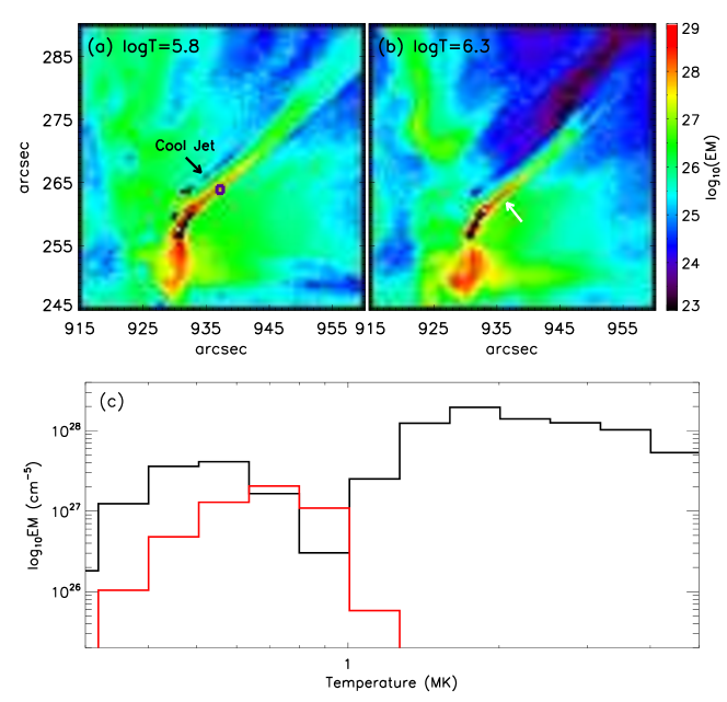
Figure 5: Top: Two maps of the active region Jet2 at 11:45 UT, at two different temperatures (log T= 5.8 and 6.3). The blue square in panel (a) is showing the location which we use for the emission analysis at the jet spire. The black arrow in panel (a) indicates a weak region of EM that we call the cool jet, the white arrow in panel (b) the hot jet. Bottom: In panel (c) the red line shows the temperature at the location of the blue box in panel (a) before the first jet ejection on April 04 2017 and the black line shows the temperature of solar active region jet at 11:45 UT.

We have investigated the distribution of the temperature and emission measure (EM) at the jet spire for all jet events. We performed the differential emission measure (DEM) analysis with the regularized inversion method introduced by Hannah & Kontar (2012) using six AIA channels (94 Å, 131 Å, 171 Å, 193 Å, 211 Å, and 335 Å. After this process we find the regularized DEM maps as a function of temperature. We use a temperature range from log T(K) = 5.5 to 7 with 15 different bins of width $\Delta$ log T = 0.1. We calculated the EM and lower limit of electron density in the jet spire using n_e = $\sqrt{EM/h}$, with $h$ the jet width, assuming that the filling factor equals unity. These EM values were obtained by integrating the DEM values over the temperature range log T(K) = 5.8 to 6.7. We chose a square box to measure the EM and density at the jet spire and at the same location before the jet activity for each jet. The example for DEM analysis of Jet2 is presented in Figure 5, which represents the DEM maps at two different temperatures, namely log T (K) = 5.8 (panel a) and 6.3 (panel b), at 11:45 UT. We investigate the temperature variation at the jet spire during the jet and pre–jet phase. During the pre–jet phase for Jet2 the log EM and the electron density values were 27.3 and 2 x 10⁹ cm^-3, whereas for the jet phase the values were 28.1 and 8.6 x 10⁹ cm^-3 respectively. Thus, during the jet evolution the EM value increased by over one order of magnitude and the electron density increased by a factor three at the jet spire. We find that the EM and density values increased during the jet phase in all six jets. The values for all jets are listed in Table 1.

2.4 Identification of observed structural elements

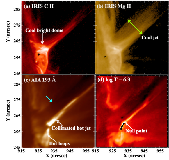
Figure 6: Example of Jet2 at 11:45 UT observed with IRIS in panel a,b and AIA 193 Å in panel c. Cool bright dome in the northern side of the null point is shown with a white arrow in panel a. We note the broad cool jet in panel b (green arrow), the collimated narrow hot jet with hot loops (white arrows) and absorption area (cyan arrow) in panel c, the null–point and the long bright current sheet (CS) are indicated by the white arrow in panel d. The black points are the saturated areas in panel d.

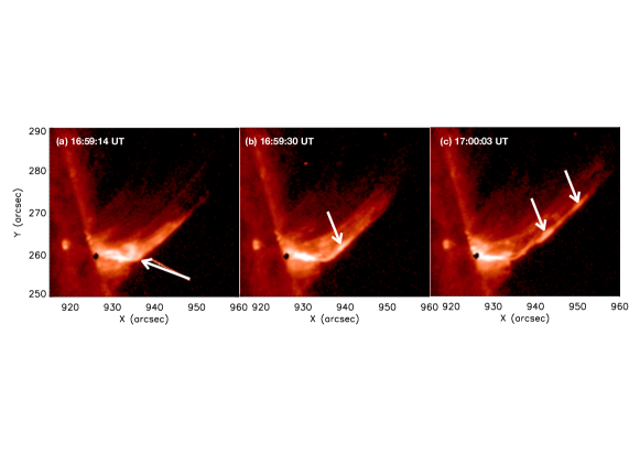
Figure 7: Kernels of brightening moving along the Jet6 observed in the IRIS SJI in CII wavelength range (see white arrows). The kernels could correspond to untwisted plasmoids.

In Section 2.2 we have discussed the morphology of the jets observed with AIA and IRIS. The region below the jet, as seen in different wavelengths, has a remarkably clear structure, resembling those discussed in theoretical models of the past years. For identification with previous theoretical work, in Figure 6 several structural elements are indicated for the case of the Jet2 observations. In IRIS CII (Figure 6, panel a) the brightenings below the jet delineate a double–chambered vault structure, with the main brightening being located in the northern part of the base of the jet. Only narrow loops are seen above the southern part of the vault in this wavelength. In the other chromospheric line, IRIS Mg II, we see (panel b) roughly the same scenario, although the general picture is rather fuzzier. The jet, in particular, is no longer narrow but formed by parallel strands issuing from the edge of the northern part of the vault, similar to a comb (Figure 6 panel b). The assumption of a double-vault structure below the jet is reinforced when checking both the hot-plasma observations (AIA 193 Å, panel c) and the temperature map obtained through the DEM analysis explained in the previous section (panel d). In those two panels, the southern loops are shown to be bright and hot structures, and the same applies to the point right at the base of the jet, where the temperature reaches $10^{6}$ K. Additionally, we observe bright kernels moving from time to time along the jets and more clearly visible in Jet4, Jet5, and Jet6. An example of kernels of brightening moving along the Jet6 in IRIS CII is presented in Figure 7. We have computed the velocities of the kernels and find that they are comparable to the mean velocities of the cool jet (45 km s^-1). The time between the ejection of two kernels is less than 2 minutes.

The foregoing structural elements seem to correspond to various prominent features in the numerical 3D models of Moreno-Insertis et al. (2008) and Moreno-Insertis & Galsgaard (2013), or in the more recent 2D models of Nóbrega-Siverio et al. (2016, 2018), all of which study in detail the consequences in the atmosphere of the emergence of magnetized plasma from below the photosphere. One can identify the bright and hot plasma apparent in the observations at the base of the jet with the null point and CS structures resulting in those simulations (see the scheme in Figure 11, right panel): the collision of the emerging magnetized plasma with the preexisting coronal magnetic system leads, when the mutual orientation of the magnetic field is sufficiently different, to the formation of an elongated CS harboring a null point and to reconnection. As a next step in the pattern identification, the hot plasma loops apparent in the southern vault in the AIA 193 Å image and the temperature panels of Figure 6 should correspond to the hot post-reconnection loop system in the numerical models (as apparent in Figures 3 and 4 of the paper by Moreno-Insertis et al. 2008, or along the paper by Moreno-Insertis & Galsgaard 2013). On the other hand, the northern vault appears dark in AIA 193 Å, and has lower temperatures in the DEM analysis. This region could then correspond to the emerged plasma vault underlying the CS in the numerical models: the magnetized plasma in that region is gradually brought toward the CS where the magnetic field is reconnected with the coronal field.

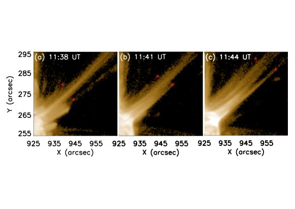
Figure 8: The evolution of cool plasma material along both sides of the hot jet (Jet2) in IRIS MgII wavelength. The red star shows the leading edge of the cool material ejecting with an average speed of 45 km s^-1.

Additional features in the observation that fit in the foregoing identification are the following:
(a) As time proceeds the northern chamber decreases in size while the southern chamber grows. In our observations in the beginning phase of the jets (for instance; jet2 at 11:30 UT) the area of the northern and southern vaults is 1.4 x 10¹⁸ and 1.16 x 10¹⁸ cm², respectively, and during the jet phase (11:47 UT), they become $1.05\times 10^{18}$ and $2.2\times 10^{18}$ cm², respectively. This suggests that while the reconnection is occurring, the emerging volume is decreasing whereas the reconnected loop domain grows in size, as in the emerging flux models (Moreno-Insertis et al., 2008; Moreno-Insertis & Galsgaard, 2013; Nóbrega-Siverio et al., 2016).
(b) A major item for the identification of the observation with the flux emergence models is the possibility that we also observe a wide, cool and dense plasma surge ejected in the neighborhood of the vault and jet complex (see movie in C II attached as MOV2). This wide laminar jet is observedin the Mg II IRIS filter as an absorption sheet parallel to the hot jet in AIA 193 Å. The evolution of the cool material along both sides of the hot jet in the IRIS Mg II channel is presented in Figure 8 and the leading edge of the cool part is indicated by red stars. The cool ejection is generally less collimated than the hot jet and is seen to first rise and then fall, similarly to classical H$\alpha$ surges. The velocities measured along the cool sheet of plasma in Mg II are $\approx$ 45 km s^-1. The ejection of cool material next to the hot jets is a robust feature in different flux emergence models (Yokoyama & Shibata, 1996; Moreno-Insertis et al., 2008; Nishizuka et al., 2008; Moreno-Insertis & Galsgaard, 2013; MacTaggart et al., 2015; Nóbrega-Siverio et al., 2016, 2017, 2018). The cool plasma in the models is constituted by matter that has gone over from the emerged plasma domain to the system of reconnected open coronal field lines without passing near the reconnection site, that is, just by flowing, because of flux freezing, alongside the magnetic lines that are being reconnected at a higher level in the corona. All those models report velocities which match very well the observed value quoted above.
(c) The observed kernels in Figure 7 could be plasmoids created in the CS during the reconnection process. In some of the flux emergence models just discussed, plasmoids are created in the CS domain (see, for example Moreno-Insertis & Galsgaard 2013), and they are hurled out of the sheet probably via the melon-seed instability (Nóbrega-Siverio et al., 2016), even though they are not seen to reach the jet region. On the other hand, in the 2D jet model by Ni et al. (2017), plasmoids are created in the reconnection site that maintain their identity when rising along the jet spire, possibly because of the higher resolution afforded by the Advanced Mesh Refinement used in the model; this is in agreement with the behavior noted in the present observations as well as in the previous observations of Zhang & Ji (2014) and Zhang et al. (2016) mentioned in the introduction. Plasmoids are also generated in the model by Wyper et al. (2016), which is a result of footpoint driving of the coronal field rather than flux emergence from the interior. On the other hand, the formation of the kernels could follow the development of the Kelvin–Helmholtz instability (KHI). The KHI can be produced when two neighboring fluids flow in same direction with different speed (Chandrasekhar, 1961). This instability may develop following the shear between the jet and its surroundings. For details about this sort of process in jets and CMEs see the review by Zhelyazkov et al. (2019).
(d) The main brightening at the top of the two vaults seems to be changing position systematically in the observations. There is a shift in the south–west direction as time advances, and the same displacement is apparent in AIA 131 Å (see Figures 2 and 4), possibly marking the motion of the reconnection site. Such type of observations are also reported in the study of Filippov et al. (2009). This shift may be used to compare with the drift of the null point position detected in the MHD models.

(e) We also notice a significant rise of the brighter point (null point) between different jet events. The rise of the reconnection site as the jet evolution advances has been found in the MHD emerging flux models of Yokoyama & Shibata (1995); Török et al. (2009). In the present case, it may be because during each jet event the reconnection process causes a displacement of the null point and jet spine. In this way the next jet event occurs in a displaced location as compared with the previous jet. This could indicate that the magnetic field configuration has some reminiscences of the earlier reconnection and behaving in the same manner afterwards. Another possible reason for this shifting could be as a result of the interaction between different quasi–separatrix layers (QSLs) as suggested by Joshi et al. 2017b. However, in the present case because of the limb location of the active region, we could not compute the QSL locations.

3 Oscillations before the jet activity

In §2.2 we mentioned that before and in between the six main jets we also observed many small jet-like ejections, with length less than $10$ Mm. Also, in the AIA 131 Å movie we clearly see many episodic brightenings related to the small jets. In the present section we would like to investigate different properties, like the periodicity, of these features. To that end, we select a square of size $4\times 4$ arcsec at the base of the jets where the intensity is maximum, in the AIA 131 Å data, as shown in Figure 2 and calculate the mean intensity inside the square in the AIA 131 Å channel. We compute the relative intensity variation in the base, after normalization by the quiet region intensity. We find that the oscillations start at the jet base some 5–40 min before the main jet activity.

Figure 9 shows the intensity distribution at the jet base for all the jets before and during the jet eruption and the pre–jet phase is shown in between two vertical red dashed lines. The right red dashed lines indicate the starting time of the main jets. The blue arrows indicate the time of the maximum elongation of the main jets. We note that the maximum of the brightening at the jet base does not always coincide exactly with the start of the jet neither with the maximum extension time. In most of the cases the maximum brightening occurs before the peak time of the jets by a few minutes. For the smaller jets it is nearly impossible to compute the delay between brightenings and jets. They appear to be in phase with the accuracy of the measurements.

To calculate the time period of these pre–jet oscillations, we apply a wavelet analysis technique. For the significance of time periods in the wavelet spectra, we take a significance test into account and the levels higher than or equal to 95% are labeled as real. The significance test and the wavelet analysis technique is well described by Torrence & Compo (1998). The cone of influence (COI) regions make an important background for the edge effect at the start and end point of the time range (Tian et al., 2008; Luna et al., 2017).

Table 1: Physical parameters of six studied hot jets.

Jet	Jet start	Jet peak	Max	Average	T	EM	Oscillation
no.	time	time	height	speed		(1028	period
	(UT)	(UT)	(Mm)	(km s-1)	(MK)	cm${}^{-5})$	(min)
1	10:15	10:22	80	210	1.4	1.4	6.0
2	11:46	11:47	50	245	1.8	1.9	1.5
3	13:54	13:55	40	265	1.4	1.5	2.5
4	14:12	14:15	50	250	1.8	1.1	2.0
5	15:23	15:25	55	235	1.8	1.3	4.0
6	16:57	17:00	70	220	1.8	2.0	2.5

The wavelet analysis of the intensity fluctuation at the jet base shows that the oscillation period for these pre–jet intensity varies between 1.5 min and 6 min; the current values obtained are presented in the last column of Table 1. An example of wavelet spectrum for the pre–jet activity for Jet2 is presented in Figure 10 (a). The COI region is the outer area of the white parabolic curve.The global wavelet spectrum in panel (b) shows the distribution of power spectra over time. Bagashvili et al. (2018) investigated the intensity at the base of several jets issued in a coronal hole and obtained similar results concerning the periodicity and duration of the oscillations.

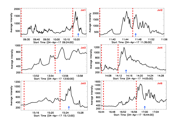
Figure 9: Intensity distribution during pre–phase of recurrent jets at the base of each jet in AIA 131 Å. The location of the jet base of each jet is displayed in Figure 2 (see red squares). In each panel, a blue arrow indicates the peak phase of the main jet. The small intensity peaks before each main jet are related to small jet ejections (10 Mm height) coming from the same location. The two vertical red dashed lines in each panel show the duration of the pre–jet intensity oscillation that is used for the wavelet analysis.

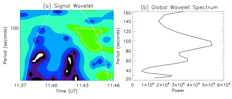
Figure 10: Panel (a): An example of wavelet spectrum for the pre–jet intensity oscillations for Jet2. The solid thick white contours (around the green surface) are the regions with the value of wavelet function larger than the 95% of its maximum value. The area which is outside the parabolic COI is the region where the wavelet analysis is not valid. Panel (b): Global wavelet spectra for the distribution of power over time. The highest peak is corresponding to the time period of the pre–jet intensity oscillations, i.e. 1.5 min for Jet2.

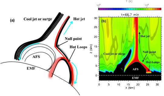
Figure 11: Panel (a): Schematic view of the 3D jet derived from Moreno-Insertis et al. (2008), showing the location of the null point, the cool surge and the hot loops next to the AFS. The cyan arrows indicate the direction of the flows. The red lines indicate the presence of hot plasma. The black lines are magnetic field lines. Panel (b): Temperature map of one of the numerical experiments by Nóbrega-Siverio et al. (2017, 2018) showing the hot jet and the cool surge (an animation of this panel is available online). In both panels, the region of the convection zone where the new magnetic flux has emerged (EMF) is also indicated.

4 Discussion and conclusion

This paper presents observations concerning the structure, kinematics, and pre–jet intensity oscillations of six major jets that occurred on April 04, 2017 in active region NOAA 12644. The discussion is based on the observational data from AIA and IRIS. A brief summary of our main results is as follows:

1. All the jets show pre–jet intensity oscillations at their base accompanied by smaller jets. The period of the oscillation ranges from 1.5 to 6 min.

2. The jets are issued from a canopy-like structure with two vaults delineated by the brightenings seen in the different wavelengths. One of the vaults harbors hot loops as seen in the EUV AIA filters and also in IRIS C II wavelength. The hot jets are accompanied by laminar cool surge–like jets visible in IRIS Mg II and C II wavelengths.

3. The spatial and temporal pattern of brightenings in the various wavelengths show clear similarities with the two- and three-dimensional numerical models of Moreno-Insertis et al. (2008); Moreno-Insertis & Galsgaard (2013) and Nóbrega-Siverio et al. (2016). The high brightening overlying the two vaults in the observations, in particular, is suggestive of the null point and CS complex in the models; the two vaults would then correspond to the domains occupied by the emerging plasma and the reconnected hot loops, respectively, in the models.

4. The cool surge-like jets visible in the IRIS images and in absorption in AIA filters may be the counterpart to the cool ejections that naturally accompany the flux emergence models. Further observed features that are present in flux emergence models are: the ejection of bright kernels from the region identified as the reconnection site, and the shift in the reconnection site towards the south–west direction.

In the following, a discussion of those results is provided:

A first significant finding of this study is the observation of pre–jet activity, in particular in the form of oscillatory behavior. Earlier authors had studied the pre–jet activity of quiet region jets observed in the hot AIA filters (Bagashvili et al., 2018). The jets studied by those authors had their origin in coronal bright points and the bright points showed oscillatory behavior before the onset of jet activity. They reported periods for the pre–jet oscillations of around 3 mins. Our study deals with active region jets, instead, also observed in the hot filters of AIA and we find an oscillatory behavior of the intensity in a time interval of 5–40 min prior to the onset of the jet. The period of the intensity oscillation is in the range 1.5–6 min. These values are consistent with the results reported by Bagashvili et al. (2018). They are also close to typical periods of acoustic waves in the magnetized solar atmosphere. This indicates that acoustic waves may be responsible for these observed periods in the occurrence of jets (Nakariakov & Verwichte, 2005). Quasi-oscillatory variations of intensity can also be the signature of MHD wave excitation processes which are generated by very rapid dynamical changes of velocity, temperature and other parameters manifesting the apparent non-equilibrium state of the medium where the oscillations are sustained (Shergelashvili et al., 2005, 2007; Zaqarashvili & Roberts, 2002). In 3D reconnection regions like the quasi-separatrix layers, a sharp velocity gradient is likely to be present. The impulsiveness of the jets could lead to such MHD wave excitation. The fast change of the dynamics and thermal parameters at these reconnection sites should be checked when possible to prove the interpretation of the intensity oscillation by MHD waves. The observed brightness fluctuations could also be due to the oscillatory character of the reconnection processes that lead to the launching of the small jets. Oscillatory reconnection has been found in theoretical contexts in two dimensions (Craig & McClymont, 1991; McLaughlin et al., 2009; Murray et al., 2009). The latter authors, in particular, studied the emergence of a magnetic flux rope into the solar atmosphere endowed with a vertical magnetic field. As the process advances, reconnection occurs in the form of bursts with reversals of the sense of reconnection, whereby the inflow and outflow magnetic fields of one burst become the outflow and inflow fields, respectively, in the following one. The period of the oscillation covers a large range, 1.5 min to 32 min. They concluded that the characteristics of oscillatory reconnection and MHD modes are quite similar. However, that model is two-dimensional and it is not clear if the oscillatory nature of the reconnection can also be found in general 3D environments.

A second significant point in our study is the comparison of the observations of the structures and time evolution of the jet complex with numerical experiments of the launching of jets following flux emergence episodes from the solar interior. Structures like the double-vault dome with a bright point at the top where the jets are initiated as seen in the hot AIA channels and also in the high-resolution IRIS images mimic the structures found in the numerical simulations of Moreno-Insertis et al. (2008) and Moreno-Insertis & Galsgaard (2013), who solved the MHD equations in three dimensions to study the launching of coronal jets following the emergence of magnetic flux from the solar interior into the atmosphere; they also have similarities with the more recent experiments, in two dimensions, of Nóbrega-Siverio et al. (2016), obtained with the radiation-MHD Bifrost code (Gudiksen et al., 2011). In the 3D models, the jet is launched along open coronal field lines that result from the reconnection of the emerged field with the preexisting ambient coronal field. Underneath the jet, two vault structures are formed, one containing the emerging cool plasma and the other a set of hot, closed coronal loops resulting from the reconnection. Overlying the two vaults one finds a flattened CS of Syrovatskii type, which contains hot plasma and where the reconnection is occurring. The field in the sheet has a complex structure with a variety of null points; in fact, in its interior, plasmoids, with the shape of tightly wound solenoids, are seen to be formed. The reconnection is of the 3D type, in broad terms of the kind described in the paper by Archontis et al. (2005). A vertical cut of the 3D structure, as in Figure 4 of the paper by Moreno-Insertis et al. (2008), clearly shows the two vaults with the overlying CS containing the reconnection site and with the jet issuing upwards from it. The figures in that paper contained values for the variables as obtained solving the physical equations; a scheme of the general structure is provided here as well (Figure 11, left panel). As the reconnection process advances, the hot-loop vault grows in size whereas the emerged-plasma region decreases, very much as observed in the present paper.

An interesting feature in the observations is the tentative detection of a surge-like episode next to the jet apparent in the IRIS Mg-II time series in a region that appears dark, in absorption, in the AIA 193 Å observations. This ejection of dense and cool plasma next to the hot jet, with the cool matter rising and falling, like in an H$\alpha$ surge, also occurs naturally both in the 3D and 2D numerical models cited above (and was already introduced by Yokoyama & Shibata 1995 in an early 2D model). The phenomenon has been studied in depth by Nóbrega-Siverio et al. (2016, 2017, 2018) using the realistic material properties and radiative transfer provided by the Bifrost code, which, in particular, facilitate the study of plasma at cool chromospheric temperatures. A snapshot of one of the experiments by those authors showing a temperature map and with indication of some major features is given in Figure 11 (right panel). In their model, the magnetic field can accelerate the plasma with accelerations up to $100$ times the solar gravity for very brief periods of time after going through the reconnection site because of the high field line curvature and associated large Lorentz force. In the advanced phase of the surge, instead, the cool plasma basically falls with free-fall speed, just driven by gravity, as had been tentatively concluded in observations (see Nelson & Doyle 2013). The velocities obtained from the observations in the present paper broadly agree with those obtained in the numerical models.

We conclude that our observations of the six EUV jets and surges constitute a clear case-study for comparison with the experiments developed to study flux emergence events such as the MHD models of Moreno-Insertis et al. (2008); Moreno-Insertis & Galsgaard (2013); Nóbrega-Siverio et al. (2016). Many observed structures were identified in their models: the reconnection site with two vaults, hot jets accompanied by surges, ejections of plasmoids in parallel with the development of the cool surges; the velocity of the hot jets (250 km ^-1) and of the cool surge (45 km s^-1), in particular, fit quite well with the predicted velocity in the models.

The similarities between the observations and the numerical models based on magnetic flux emergence are no proof, of course, that the observed jets are directly caused by episodes of magnetic flux emergence through the photosphere into the corona: given the limb location of the current observations, there is no possibility of ascertaining whether magnetic bipoles are really emerging at the photosphere and causing the jet activity. However, a jet from this active region that occurred on March 30, 2017, was also studied by Ruan et al. (2019) ; on that date, the active region was at the solar disk and the photospheric magnetic field measurements were reliable. Those authors reported that flux emergence episodes were continually occurring in the active region at that time. Although there can be no direct proof through magnetograms, it is likely that flux emergence continued to take place as the active region remain being strong and complex until April 04, 2017. Important jets were also observed the day before when the region was close to the limb with AIA and in H$\alpha$ but we have no IRIS data to observe the fine structures and the null point.

In the future it will be interesting to observe such events with double vault in multi-wavelengths with AIA and IRIS but on the disk to be able to detect magnetic flux emergence with HMI magnetograms. It will also be very interesting to have the spectra of IRIS just on the reconnection site. We would like to detect with high accuracy the formation of plasmoids in the current sheet using the spectral capabilities of IRIS. Such kind of observations can serve to validate the numerical experiments of the theoretical scientists.