Soil searching by an artificial root

Abstract

We model an artificial root which grows in the soil for underground prospecting. Its evolution is described by a controlled system of two integro-partial differential equations: one for the growth of the body and the other for the elongation of the tip. At any given time, the angular velocity of the root is obtained by solving a minimization problem with state constraints. We prove the existence of solutions to the evolution problem, up to the first time where a "breakdown configuration" is reached. Some numerical simulations are performed, to test the effectiveness of our feedback control algorithm.

1 Introduction

We consider a mathematical model for a robotic root, which is able to move inside a medium by growing and bending. These artificial roots are made of a tubular body, a growing head (realized by depositing new material adjacent to the tip) and a sensorized tip that commands the robotic behaviors. These mechanisms are inspired by the so-called apical growth or elongation from the tip process in plant roots: newly generated cells by mitosis move from the meristematic region near the root apex to the elongation region where they expand axially, while mature cells of the root remain stationary and in contact with the soil. Root-like devices, made of deformable materials (continuum soft robots), are particularly efficient to act in a space-constrained and unstructured environment (e.g. exploring uncertain terrains searching for life or resources in the soil, accomplishing predetermined tasks in environments with solid obstacles [11, 18], or performing minimally invasive surgery [6]) and to interact more safely with humans (e.g. rescuing people trapped by earthquakes or avalanches, in hazardous areas).

Within the growing interest in biologically inspired technologies [15], robots inspired by the stems and roots of plants are receiving a distinctive attention because plants are the most efficient and compliant living organisms for soil exploration. Therefore, their remarkable features can be exploited in artificial systems to ensure energy efficiency and minimize friction while exploring and searching ( see ([12, 16, 17, 19]).

In the present paper we provide a mathematical analysis of two simple models of continuum robotic roots with apical growth, which explore the soil in order to reach a certain target. This study should help in developing better control strategies and optimizing the implementation of these new technologies.

In the same spirit of the models introduced in [1, 5] for the growth of a plant stem or a vine, at each time $t$ the robotic root will be described by a curve $\gamma(t,\cdot)$ in 3-dimensional space. The model takes into account the fact that the artificial root is able to bend when the soil is too hard or when it finds an obstacle, and it can even contract when it is not able to outflank an hindrance. The evolution of the robotic root is governed by a system of two partial differential equations, one for the growth of the body, and the other one for the extension of the tip. The angular velocity of the root is obtained as solution of an optimization problem with state constraint. In fact, it is physically meaningful that the robot bends minimizing the instantaneous deformation energy and the cost to move sand or to drill in high-density regions.

For a general description of plant and root development from a biological point of view we refer to [13] and [9], respectively, while for a mathematical theory of biological growth we refer to [2, 3, 10].

The remainder of the paper is organized as follows: in Section 2 we introduce the basic models for the evolution of our artificial root. In Sections 2.1 and 2.2 we describe respectively a rigid and an elastic model for the robot, introducing a restarting procedure when it is no longer able to grow because of an obstacle. Most of our analysis is focused on the elastic model, since it is the most realistic, and it provides more interesting theoretical challenges. This is covered in Section 3. Section 4 is devoted to the construction of a solution to the evolution problem. Finally, in Section 5 we present some numerical simulations.

2 Modeling the growth of an artificial root

We seek to model the movement of an artificial root, which penetrates the ground searching for water, chemical compounds, cavities where earthquake survivors may be trapped, etc$\ldots$

For this purpose, we need to assign:

• An equation describing the scalar velocity at which the length of the root grows.

• An equation describing how the orientation ${\bf k}(t)$ of the tip of the root changes in time.

• A rule determining when the growth stops, the root shrinks to an earlier configuration, and then starts growing in a new direction.

2.1 A rigid root

In this first rigid model we assume that the root grows and bends from the tip but the portion of the root that has already grown does not move. In this case, apart from restarting times, the growth can be determined by a second order ODE.

1. At any time $t$, the root will be described by a ${\cal C}^{1,1}$ curve with values in ${\mathbb{R}}^{3}$:

$$s~{}\mapsto~{}\gamma(t,s),\qquad s\in[0,t],$$ (2.1)

parameterized by arc-length. The point $\gamma(t,s)$ denotes the position at time $s\in[0,t]$ of the tip of the root grown until time $t$. Since we are assuming that when the root apex grows no deformation of the rest of the body is undertaken, we have

$$\gamma_{t}(t,s)=0\qquad\hbox{for all}~{}\ s\in[0,t]\,.$$ (2.2)

For simplicity we assume that the root grows at unit speed, i.e. that $|\gamma_{s}(t,s)|=1$ for all $s\in[0.t]$, so that at time $t$ its length is simply $\ell(t)=t$. We denote by

$${\bf k}(t,s)~{}\doteq~{}\gamma_{s}(t,s)$$ (2.3)

the unit tangent vector to the curve. 2. For convenience we shall denote by

$$P(t)~{}\doteq~{}\gamma(t,t),\qquad\qquad{\bf k}(t)~{}\doteq~{}{\bf k}(t,t)~{}=~{}\gamma_{s}(t,t)$$ (2.4)

respectively the position and the orientation of the root tip.

Two types of control will be implemented. Namely:

• At every time $t$, the orientation of the tip is modified.

• At a finite number of times $0<t_{1}<t_{2}<\cdots$, if the root hits an obstacle, a restarting procedure is adopted and growth is restarted in a different direction.

3. At any time $t$, we assume that the direction ${\bf k}(t)$ of the root tip can change, subject to a maximum possible curvature. Namely,

$$\dot{\bf k}(t)~{}=~{}{\bf u}(t)\times{\bf k}(t),\qquad\qquad|{\bf u}(t)|~{}\leq~{}\kappa_{0}$$ (2.5)

Here ${\bf u}(\cdot)$ is a measurable control function, describing the angular velocity at which we bend the tip of the root. 4. We now introduce a feedback rule, assigning the control ${\bf u}$ in terms of the position of the tip. Toward this goal, we consider two scalar functions.

• A function $\phi:{\mathbb{R}}^{3}\mapsto{\mathbb{R}}$, given at the beginning and never modified afterwards. Roughly speaking one may think of $\phi(x)$ as the expected distance from a (random) target.

• A function $\psi:{\mathbb{R}}^{3}\mapsto{\mathbb{R}}$, measuring a kind of closeness to previously reached points. A bit more precisely, if $\Gamma(t)$ is the union of all points reached by the artificial root during previously failed attempts, we could define

  $$\psi(x)~{}\doteq~{}\int_{y\in\Gamma(t)}e^{-|x-y|}\,dy,$$ (2.6)

In view of (2.2), (2.4), (2.5), the growth of the root can then be described by

$$\dot{P}(t)~{}=~{}{\bf k}(t),\qquad\qquad\dot{\bf k}(t)~{}=~{}{\bf u}(t)\times{\bf k}(t),$$ (2.7)

where the control vector ${\bf u}$ is determined by

$${\bf u}(t,P(t))~{}=~{}\hbox{arg}\!\min_{|\omega|\leq\kappa_{0}}\Big{\langle}\omega\times{\bf k}(t)\,,\,\nabla\phi(P(t))+\nabla\psi(P(t))\Big{\rangle}.$$ (2.8)

Note: in (2.6), instead of $e^{-|x-y|}$, one could use some other kernel $K(|x-y|)$, where $s\mapsto K(s)$ is a smooth, decreasing function.

In some cases, the control in (2.8) may not be unique. To achieve a well posed evolution equation, it is convenient to replace (2.8) with

$${\bf u}(t,P(t))~{}=~{}\hbox{arg}\!\min_{|\omega|\leq\kappa_{0}}\Big{\{}\big{\langle}\omega\times{\bf k}(t)\,,\nabla\phi(P(t))+\nabla\psi(P(t))\big{\rangle}+\varepsilon|\omega|^{2}\Big{\}}.$$ (2.9)

The strict convexity of the right hand side yields a unique minimizer, depending Lipschitz continuously on $P$. Of course, other approximations are possible, with ${\cal C}^{\infty}$ dependence on ${\bf k},\nabla\phi,\nabla\psi$.

Having done this, the local existence and uniqueness of solutions to the evolution problem (2.7) is trivial.

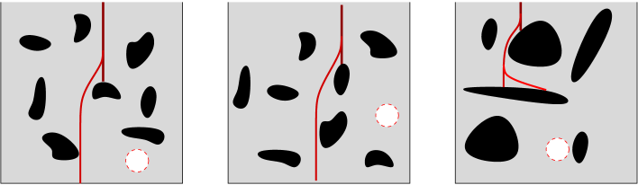
Figure 1: Rocks with different average sizes should determine different restarting strategies. The white circles denote the targets.

5. In addition, there must be a rule prescribing when the growth should stop and the root should go back to a previous configuration, and restart.

We denote by $\gamma_{i}(\cdot,\cdot)$ the curve constructed at the $i$-th trial run, and write $P_{i}(t)=\gamma_{i}(t,t)$ for the position of the tip of this curve at time $t$. The $i$-th curve starts with length $t_{i}^{-}$ and grows up to a maximum length $t_{i}^{+}$.

Here $h:{\mathbb{R}}^{3}\mapsto[0,1]$ is some scalar function, not known a priori, accounting for the “hardness" of the soil. For example, $h=0$ when the soil offers no resistance (say, inside a crack), while $h>\!>1$ along an impenetrable obstacle (say, a wall).

A reasonable stopping rule is then

$$t_{i}^{+}~{}\doteq~{}\max\Big{\{}t>t_{i}^{-}\,;~{}~{}h(P(t))\leq h_{0}\Big{\}}\,.$$ (2.10)

Here $h_{0}>0$ is a threshold value, assigned a priori. The idea is that, if the tip of the root encounters very hard soil or a rock, it is better go back and restart in another direction.

The restarting procedure must also be carefully defined. Calling $t_{i}^{+}$ the length of the root when we decide to restart, we choose a new length $t_{i+1}^{-}<t_{i}^{+}$ and set

$$\gamma(s,t_{i+1}^{-})~{}=~{}\gamma(s,t_{i}^{+})\qquad\qquad s\in[0,t_{i+1}^{-}].$$ (2.11)

In general, the new length will be determined by a restarting function:

$$t_{i+1}^{-}~{}=~{}R\Big{(}t_{i}^{+},t_{i}^{-},\psi(P(t_{i}^{+}))\Big{)}.$$ (2.12)

By (2.12), we are saying that the amount by which the root shrinks depends on

• the length $t_{i}^{+}$ and the change in the length $t_{i}^{+}-t_{i}^{-}$, achieved during the previous failed attempt,

• the density $\psi(P(t_{i}^{+}))$, measuring how much the region near $P(t_{i}^{+})$ has already been explored.

A first basic example of restarting function that one can consider is

$$R_{1}\Big{(}t_{i}^{+},t_{i}^{-},\psi(P(t_{i}^{+}))\Big{)}~{}=~{}t_{i}^{+}+c\Big{(}e^{-\psi(P(t_{i}^{+}))}-1\Big{)}\Big{(}t_{i}^{+}-t_{i}^{-}\Big{)}$$ (2.13)

with $c>1$. This can be interpreted as follows: if the value of $\psi(P(t_{i}^{+}))$ is large (which means that $P(t_{i}^{+})$ is close to many trajectories already explored in previous attempts), then we need to go back a strictly greater quantity than the last change of length $t_{i}^{+}-t_{i}^{-}$, if $\psi(P(t_{i}^{+}))$ is small, we do not need to restart so far from the last starting point $P(t_{i}^{-})$.
As an alternative restarting function, we propose:

$$R_{2}\Big{(}t_{i}^{+},t_{i}^{-},\psi(P(t_{i}^{+}))\Big{)}~{}=~{}t_{i}^{+}+c\Big{(}1+2\rho\chi_{[0,\rho]}(|P(t_{i}^{+})-P(t_{i}^{-})|)\Big{)}\Big{(}e^{-\psi(P(t_{i}^{+}))}-1\Big{)}\Big{(}t_{i}^{+}-t_{i}^{-}\Big{)}.$$ (2.14)

Compared with (2.13), we have now inserted a factor measuring the length of the last attempt. This is motivated by the fact that, if the last elongation is small (in the interval $[0,\rho]$, for some fixed threshold value $\rho>0$), then probably the root has not enough space to move, therefore it is reasonable to retreat back by a length much greater then $t_{i}^{+}-t_{i}^{-}$.

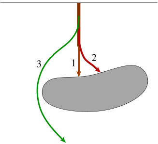
Figure 2: Three attempts at growing a root past a rock.

Remark 2.1.

In practice, the rate of growth of the root will likely depend on the hardness of the soil at the tip. In other words, at time $t$ the total length will not be $\ell(t)=t$. Rather, it may increase at a rate

$$\dot{\ell}(t)~{}=~{}{1\over 1+h\bigl{(}\gamma(\ell(t))\bigr{)}}\,,$$ (2.15)

so that

$$\dot{P}(t)~{}=~{}{d\over dt}\gamma(t,\ell(t))~{}=~{}{{\bf k}(\ell(t))\over 1+h\bigl{(}\gamma(\ell(t))\bigr{)}}\,.$$ (2.16)

This more general case can be reduced to the previous setting by using a rescaled time $\tau(t)=\ell(t)$. In this way, as in [1, 4, 5], we can assume that at time $\tau$ the curve $\gamma(\tau,\cdot)$ has length $\tau$. This length thus increases at unit rate.

2.2 A flexible root

In the previous model the growing root was completely rigid. Since the previously constructed portions of the root do not move, the equation of growth reduces to a simple ODE.

We now consider an alternative model, where the root is allowed to change its shape, in response to obstacles in the surrounding environment. The instantaneous deformation of the root is determined as a minimizer of an elastic deformation energy, plus a cost for displacing the nearby soil.

Let $s\mapsto\gamma(t,s)$, $s\in[0,t]$, be an arc-length parameterization of the root at time $t$. Moreover, let $h=h(x)\geq 0$ be a function describing the hardness of the soil at the point $x$, and fix a constant $\alpha>0$. In practice, one may think to acquire information about the rigidity of the soil in the surrounding of the robotic root by means of sensor located along the body of the root.

If the soil around the tip is very hard, or if obstacles are encountered, the root may be forced to bend. As in [4, 5], introducing a field of angular velocities $\omega(t,\cdot)$, the evolution of the curve $\gamma$ is described by

$$\gamma_{t}(t,s)~{}=~{}\int_{0}^{s}\omega(t,\sigma)\times\bigl{(}\gamma(t,s)-\gamma(t,\sigma)\bigr{)}\,d\sigma,$$ (2.17)

while, with the same setting as in (2.3)-(2.4), we have

$$\dot{P}(t)~{}=~{}{\bf k}(t)+\int_{0}^{t}\omega(t,\sigma)\times\bigl{(}\gamma(t,s)-\gamma(t,\sigma)\bigr{)}\,d\sigma.$$ (2.18)

As in (2.5), this equation must be supplemented with a boundary condition describing how the orientation of the tip changes in time:

$$\dot{\bf k}(t)~{}=~{}\left({\bf u}(t)+\int_{0}^{t}\omega(t,\sigma)\,d\sigma\right)\times{\bf k}(t).$$ (2.19)

Here the feedback control ${\bf u}(t)$ can be chosen as in (2.9), in order to approach the target as fast as possible. Notice that the integral term in (2.19) accounts for the change in the orientation of the tip coming from the elastic deformation.

At each given time $t$, following [4] we assume that the field of angular velocities $\omega(\cdot)$ in (2.17)–(2.19) is determined by an instantaneous minimization problem, which we now describe.

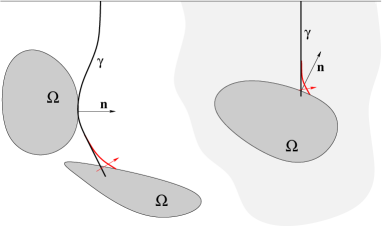
Figure 3: By an infinitesimal elastic deformation, the curve $\gamma$ is kept outside the obstacle. Left: outside the obstacle there is empty space. Right: the obstacle is surrounded by softer soil.

Assume that the external environment consists of soil whose hardness is described by a scalar function $h=h(x)\geq 0$, together with impenetrable obstacles, whose union we denote by $\Omega\subset{\mathbb{R}}^{3}$. We assume that $\Omega$ is an open set with ${\cal C}^{2}$ boundary $\partial\Omega$. The unit outer normal vector at a point $x\in\partial\Omega$ will be denoted by ${\bf n}(x)$. At a contact point $\gamma(t,s)\in\partial\Omega$, this unit outer normal is denoted by

$${\bf n}(t,s)~{}\doteq~{}{\bf n}(\gamma(t,s)).$$

In our model, the angular velocity $\omega(t,\cdot)\in{\bf L}^{2}([0,t])$ is determined as the solution to the following optimization problem.

• Given $\gamma(t,\cdot)\in{\bf H}^{2}([0,t])$, find an angular velocity $\omega\in{\bf L}^{2}([0,t])$ which minimizes the functional

  $$\begin{array}[]{rl}J(\omega)&\displaystyle\doteq~{}\int_{0}^{t}|\omega(s)|^{2}\,ds+\int_{0}^{t}h(\gamma(t,s))\cdot\Big{|}\gamma_{t}(t,s)\times{\bf k}(t,s)\Big{|}\,ds+\alpha\,h(P(t))\cdot\big{\langle}\dot{P}(t),{\bf k}(t)\big{\rangle}_{+}\\[11.38109pt] &=~{}J_{1}(\omega)+J_{2}(\omega)+J_{3}(\omega)\,.\end{array}$$ (2.20)

  Here $\gamma_{t}$ and $\dot{P}$ are recovered from $\omega(\cdot)$ by the formulas (2.17)-(2.18), while

  $$\langle{\bf v},{\bf w}\rangle_{+}~{}\doteq~{}\max\{\langle{\bf v},{\bf w}\rangle\,,~{}0\}$$

  denotes the positive part of an inner product. The global minimizer of the functional (2.20) is sought under the constraints

  $$\Big{\langle}{\bf n}(t,s)\,,\,\gamma_{t}(t,s)\Big{\rangle}~{}\geq~{}0\qquad\hbox{for all $s$ such that $\gamma(t,s)\in\partial\Omega$}.$$ (2.21)

  In the case where $P(t)\doteq\gamma(t,t)\in\partial\Omega$, we impose the additional constraint

  $$\Big{\langle}{\bf n}(t,t)\,,\,\dot{P}(t)\Big{\rangle}~{}\geq~{}0.$$ (2.22)

Remark 2.2.

The three terms on the right hand side of (2.20) can be interpreted as

[elastic bending energy]  +  [soil hardness]$$\times \times$$[swept area]  +  [soil hardness][tip penetration].

The coefficient $\alpha>0$ allows to better calibrate the relative weight of these terms.

Remark 2.3.

In [4, 5], the surface of the obstacle was modeled as a smooth frictionless surface. In alternative, one could impose that there is some friction between the obstacle and the tip of the root. For example, one can impose that the tip can move only if

$$\big{\langle}{\bf n}(t,t)\,,\,{\bf k}(t,t)\big{\rangle}~{}\geq~{}\kappa_{0}\,,$$ (2.23)

for some $\kappa_{0}\in\,]-1,0]$.

Remark 2.4.

In the first model, considered in Section 2.1, the root is completely rigid, in the sense that the portion that is already grown does not change its position at any later time. On the other hand, in this second model the dynamics is more complex, because it takes into account the elasticity of the root.

The difference is only in the dynamics. The optimal control (orienting the tip in the direction where it is more likely to find the target), as well as the restarting strategy, can be chosen in the same way as in the model discussed in the first two sections.

3 Solutions to the flexible root model

From a theoretical point of view, the model with a flexible root is the most interesting. Toward a proof of well-posedness, two steps are required.

• At any time $t\geq 0$, the instantaneous growth is determined by solving a minimization problem with constraints. One needs to prove that this optimization problem admits a unique solution. Moreover, this minimizer depends continuously on the data, except when a “breakdown configuration" is reached, as in the model studied in [5].

• Following [4], one should then introduce a suitable weighted distance among root configurations, and prove that the evolution problem is well posed.

Aim of this section is to prove a local existence theorem, valid as long as a “breakdown configuration" is not reached, as shown in Fig. 4.

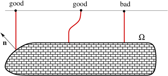
Figure 4: For the two initial configurations on the left and in the center, the constrained growth equations for the root admit a unique solution. The root configuration on the right satisfies the condition (B). In such case, the Cauchy problem is ill posed.

Definition 3.1.

We say that a curve $\gamma:[0,t_{0}]\mapsto{\mathbb{R}}^{3}\setminus\Omega$ is in a breakdown configuration w.r.t. the obstacle $\Omega$ if the following holds

• The tip $\gamma(t_{0})$ touches the obstacle perpendicularly, namely

  $$\gamma(t_{0})~{}\in~{}\partial\Omega\,,\qquad\qquad\gamma_{s}(t_{0})~{}=~{}-{\bf n}(\gamma(t_{0})).$$ (3.1)

  Moreover,

  $$\gamma_{ss}(s)~{}=0\qquad\hbox{for all $s\in~{}]0,t_{0}[\,$ such that~{}}\gamma(s)\notin\partial\Omega\,.$$ (3.2)

3.1 Determining the instantaneous velocity.

At each time $t\geq 0$, the velocity of points on the curve $\gamma(t,\cdot)$ and of the root tip $P(t)$ is determined by (2.17) and (2.18), respectively. In our model, the instantaneous bending rate $\omega(t,\cdot)\in{\bf L}^{2}([0,t]\,;\,{\mathbb{R}}^{3})$ is determined as the unique global minimizer of the functional (2.20), subject to the constraints (2.21)-(2.22). We recall that $h:{\mathbb{R}}^{3}_{-}\mapsto{\mathbb{R}}$ is a smooth scalar function, describing the hardness of the soil.

Lemma 3.2.

If $\gamma(t,\cdot)$ is not a breakdown configuration, then the functional (2.20) has a unique minimizer, subject to (2.17)-(2.18) and the constraints (2.21)-(2.22).

Proof. 1. Call ${\cal A}\subseteq{\bf L}^{2}([0,t])$ the set of angular velocities for which the constraints (2.21)-(2.22) are satisfied. Recalling (2.17)-(2.18), we observe that the maps

$$\omega(\cdot)~{}\mapsto~{}\gamma_{t}(t,\cdot),\qquad\quad\omega(\cdot)~{}\mapsto~{}\dot{P}(t)$$

are linear and affine, respectively. We thus deduce that ${\cal A}$ is a closed, affine subspace of ${\bf L}^{2}$.

Next, if $\gamma(t,\cdot)$ does not satisfy all conditions in (B), by adapting some arguments in the proof of Lemma 1 in [5] we now show that ${\cal A}$ is a nonempty set. Indeed, assume that ${\bf v}\in{\bf H}^{2}([0,t];{\mathbb{R}}^{3})$ is a velocity field produced by the obstacle reaction when $\gamma(t,\cdot)$ touches $\partial\Omega$, or a reaction due to hardness of the soil, with

$${\bf v}(0)={\bf v}^{\prime}(0)=0,\quad\quad\langle{\bf v}^{\prime}(s)~{},~{}{\bf k}(t,s)\rangle=0\quad\text{ for all }s\in[0,t],$$ (3.3)

$$\langle{\bf n}(t,s)\,,\,{\bf v}(s)\rangle\geq 0\qquad\text{if}\qquad\gamma(t,s)\in\partial\Omega\,,\quad s\in[0,t],$$ (3.4)

$$\langle{\bf n}(t,t)\,,\,{\bf v}(t)+{\bf k}(t,t)\rangle\geq 0\qquad\text{if}\quad\ \gamma(t,t)\in\partial\Omega\,.$$ (3.5)

Here ${\bf v}$ plays the role of $\gamma_{t}(t,\cdot)$, defined by (2.17). We claim that there exists a unique angular velocity field $\omega\in{\bf L}^{2}([0,t];{\mathbb{R}}^{3})$ such that

$$\|\omega\|_{{\bf L}^{2}}\leq C\|{\bf v}\|_{{\bf H}^{2}}\,,\\$$ (3.6)

$$\langle\omega(s),{\bf k}(t,s)\rangle=0\quad\quad\text{ for all }s\in[0,t]\,,$$ (3.7)

$${\bf v}(s)=\int_{0}^{s}\omega(\sigma)\times(\gamma(t,s)-\gamma(t,\sigma))d\sigma\quad\text{for all }s\in[0,t].$$ (3.8)

Notice that (3.4), (3.8) together yield (2.21), while from (2.18), (2.21) and(3.5), we recover (2.22).

To prove the Claim, using (3.3) and differentiating (3.8), we first observe that $\omega(\cdot)$ satisfies (3.8) if and only if

$${\bf v}^{\prime}(s)~{}=~{}\int_{0}^{s}\omega(\sigma)d\sigma\times{\bf k}(t,s)\quad\text{for all }s\in[0,t].$$ (3.9)

Now consider a family of orthonormal frames $\{{\bf e}_{1}(s),{\bf e}_{2}(s),{\bf e}_{3}(s)\}$ such that ${\bf e}_{1}(s)={\bf k}(t,s)$ for all $s\in[0,t]$. We seek two scalar functions $\omega_{2},\omega_{3}:[0,t]\rightarrow{\mathbb{R}}$ so that (3.8) holds with

$$\omega(s)~{}=~{}\omega_{2}(s){\bf e}_{2}(s)+\omega_{3}(s){\bf e}_{3}(s).$$ (3.10)

Notice that (3.7) is an immediate consequence of the orthogonality of the three vectors ${\bf e}_{i}(s)$.

By the orthogonality assumption in (3.7), we get two scalar functions $z_{2}$ and $z_{3}$ such that

$${\bf v}^{\prime}(s)~{}=~{}z_{2}(s){\bf e}_{2}(s)+z_{3}(s){\bf e}_{3}(s) =~{}\int_{0}^{s}\bigl{(}\omega_{2}(\sigma){\bf e}_{2}(\sigma)+\omega_{3}(\sigma){\bf e}_{3}(\sigma)\bigr{)}d\sigma\times{\bf e}_{1}(s).$$ (3.11)

Projecting respectively along ${\bf e}_{2}(s)$ and ${\bf e}_{3}(s)$ we obtain

$$z_{2}(s)=\int_{0}^{s}\langle{\bf e}_{2}(\sigma)\times{\bf e}_{1}(s),~{}{\bf e}_{2}(s)\rangle\omega_{2}(\sigma)d\sigma+\int_{0}^{s}\langle{\bf e}_{3}(\sigma)\times{\bf e}_{1}(s),~{}{\bf e}_{2}(s)\rangle\omega_{3}(\sigma)d\sigma,$$

$$z_{3}(s)=\int_{0}^{s}\langle{\bf e}_{2}(\sigma)\times{\bf e}_{1}(s),~{}{\bf e}_{3}(s)\rangle\omega_{2}(\sigma)d\sigma+\int_{0}^{s}\langle{\bf e}_{3}(\sigma)\times{\bf e}_{1}(s),~{}{\bf e}_{3}(s)\rangle\omega_{3}(\sigma)d\sigma.$$

By the property of the mixed product $\langle{\bf u},({\bf v}\times{\bf w})\rangle=\langle{\bf v},({\bf w}\times{\bf u})\rangle$, we can write

$$z_{2}(s)~{}=~{}\displaystyle\int_{0}^{s}\Big{[}\langle{\bf e}_{2}(\sigma),~{}{\bf e}_{3}(s)\rangle\omega_{2}(\sigma)+\langle{\bf e}_{3}(\sigma),~{}{\bf e}_{3}(s)\rangle\omega_{3}(\sigma)\Big{]}d\sigma\,,$$

$$z_{3}(s)~{}=~{}\displaystyle-\int_{0}^{s}\Big{[}\langle{\bf e}_{2}(\sigma),~{}{\bf e}_{2}(s)\rangle\omega_{2}(\sigma)+\langle{\bf e}_{3}(\sigma),~{}{\bf e}_{2}(s)\rangle\omega_{3}(\sigma)\Big{]}d\sigma\,.$$

Since all the function involved in $(\ref{Dec})$ are in ${\bf H}^{1}$, we can differentiate once again and obtain

$$\left\{\begin{array}[]{rl}\omega_{3}(s)&=~{}\displaystyle z_{2}^{\prime}(s)-\int_{0}^{s}\Big{[}\langle{\bf e}_{2}(\sigma),~{}{\bf e}_{3}^{\prime}(s)\rangle\omega_{2}(\sigma)+\langle{\bf e}_{3}(\sigma),~{}{\bf e}_{3}^{\prime}(s)\rangle\omega_{3}(\sigma)\Big{]}d\sigma,\\[11.38109pt] \omega_{2}(s)&\displaystyle=~{}-z_{3}^{\prime}(s)-\int_{0}^{s}\Big{[}\langle{\bf e}_{2}(\sigma),~{}{\bf e}_{2}^{\prime}(s)\rangle\omega_{2}(\sigma)+\langle{\bf e}_{3}(\sigma),~{}{\bf e}_{2}^{\prime}(s)\rangle\omega_{3}(\sigma)\Big{]}d\sigma.\end{array}\right.$$ (3.12)

This is a linear system of of Volterra integral equation, whose unique solution can be obtained by a fix point argument. Indeed, introducing the vector notation

$$U=\begin{pmatrix}\omega_{2}\\ \omega_{3}\end{pmatrix},\quad\quad Z=\begin{pmatrix}-z_{3}\\ z_{2}\end{pmatrix},$$ (3.13)

the system (3.12) can be written as

$$U(s)~{}=~{}Z^{\prime}(s)+\int_{0}^{s}B(s,\sigma)U(\sigma)d\sigma~{}\doteq~{}\mathcal{F}[Z^{\prime},U](s),$$ (3.14)

where the matrix $B(s,\sigma)$ has norm

$$|B(s,\sigma)|~{}\leq~{}2|{\bf e}_{2}^{\prime}(s)|+2|{\bf e}_{3}^{\prime}(s)|~{}\doteq~{}b(s).$$ (3.15)

The operator $\mathcal{F}$ defined at (3.14) is a strict contraction w.r.t. $U$ on the space ${\bf L}^{1}([0,T];\mathbb{R}^{2})$, with the equivalent norm

$$\|U\|~{}\doteq~{}\int_{0}^{t}\text{exp}\left\{-2\int_{0}^{s}b(\sigma)d\sigma|U(s)|\right\}|U(s)|ds.$$ (3.16)

Moreover, by the contraction mapping principle we have

$$\|U\|_{{\bf L}^{1}}\leq C_{1}\|Z^{\prime}\|_{{\bf L}^{1}}\leq C_{2}\|Z^{\prime}\|_{{\bf L}^{2}},$$ (3.17)

with $C_{1},C_{2}$ constants depending on $t$ and $b(\cdot)$. Conclusively we obtain that

$$\|U\|_{{\bf L}^{2}}^{2} \leq 2\|Z^{\prime}\|_{{\bf L}^{2}}^{2}+\int_{0}^{t}b^{2}(s)\Big{(}\int_{0}^{s}U(\sigma)\sigma\Big{)}^{2}ds$$

$$\leq 2\|Z^{\prime}\|_{{\bf L}^{2}}^{2}+2\|b\|_{{\bf L}^{2}}^{2}\|U\|_{{\bf L}^{1}}^{2}$$

$$\leq(2+2\|b\|_{{\bf L}^{2}}^{2}C_{2}^{2})\|Z^{\prime}\|_{{\bf L}^{2}}$$

hence also $\omega_{1}$ and $\omega_{2}$ are in ${\bf L}^{2}$. To conclude we just need to observe that $\|Z^{\prime}\|_{{\bf L}^{2}}=\mathcal{O}(1)\cdot\|{\bf v}\|_{{\bf H}^{2}}$ and $\|b\|_{{\bf L}^{2}}\mathcal{O}(1)\|\gamma\|_{{\bf H}^{2}}$. Condition $(\ref{th0})$ plays an essential role in uniquess of the angular velocity $\omega$, indeed without that we can produce infinitely many solution for the system $(\ref{th1})$.

2. We now observe that the functional $J$ in (2.20) is non-negative, strictly convex, and coercive on ${\bf L}^{2}$.

Let $(\omega_{n})_{n\geq 1}$ be a minimizing sequence in ${\cal A}\subseteq{\bf L}^{2}$. By coercivity, the norms $\|\omega_{n}\|_{{\bf L}^{2}}$ are uniformly bounded. By possibly extracting a subsequence, we can thus assume the weak convergence $\omega_{n}\rightharpoonup\omega^{*}$.

Since the functional $J$ is convex, it is lower semicontinuous w.r.t. weak convergence. Therefore

$$J(\omega^{*})~{}\leq~{}\liminf_{n\to\infty}J(\omega_{n})~{}=~{}\inf_{\omega\in{\cal A}}J(\omega).$$

Recalling that ${\cal A}$ is closed, we conclude that $\omega^{*}\in{\cal A}$ is a global minimizer.

Finally, the strict convexity of $J$ implies that this minimizer is unique. MM     

3.2 Solutions to the evolution problem.

Given a feedback control ${\bf u}={\bf u}(x)$ accounting for the desired bending of the tip, we can now give a precise definition of “solution" of the evolution problem describing the growth of the artificial root.

At each time $t$, the position of the root is described by a map $\gamma(t,\cdot)$ from $[0,t]$ into ${\mathbb{R}}^{3}$. Of course, the domain of this map grows with time. Following [5], it is convenient to reformulate our model as an evolution problem on a functional space independent of $t$. We thus fix $T>t_{0}$ and consider the Hilbert-Sobolev space ${\bf H}^{2}([0,T];\,{\mathbb{R}}^{3})$.

An initial data $\overline{\gamma}\doteq\gamma(t_{0},\cdot)\in{\bf H}^{2}([0,t_{0}];\,{\mathbb{R}}^{3})$ will be canonically extended to ${\bf H}^{2}([0,T];\,{\mathbb{R}}^{3})$ by setting

$$\overline{\gamma}(s)~{}\doteq~{}\overline{\gamma}(t_{0})+(s-t_{0})\overline{\gamma}^{\prime}(t)\qquad\qquad\hbox{for}~{}~{}s\in[t_{0},T]\,.$$ (3.18)

Notice that the above extension is well defined because $\overline{\gamma}(\cdot)$ and its derivative $\overline{\gamma}^{\prime}(\cdot)$ are continuous functions. In the following we shall study functions defined on a domain of the form

$${\cal D}_{T}~{}\doteq~{}\bigl{\{}(t,s)\,;~{}~{}0\leq s\leq t,~{}~{}t\in[t_{0},T]\bigr{\}},$$ (3.19)

and extended to the rectangle $[t_{0},T]\times[0,T]$ as in (3.18).

Definition 3.3.

We say that a function $\gamma=\gamma(t,s)$, defined for $(t,s)\in[t_{0},T]\times[0,T]$ is a solution to the root growth problem (2.17)-(2.19), with initial condition

$$\gamma(t_{0},s)~{}=~{}\overline{\gamma}(s),\qquad\qquad s\in[0,t_{0}],$$ (3.20)

if the following holds.

• The map $t\mapsto P(t,\cdot)$ is Lipschitz continuous from $[t_{0},T]$ into ${\bf H}^{2}([0,T];\,{\mathbb{R}}^{3})$.

• For a.e.  $t\in[t_{0},T]$ the partial derivative $\partial_{t}\gamma(t,\cdot)$ is given by

  $$\gamma_{t}(t,s)~{}=~{}\int_{0}^{s}\omega(t,\sigma)\times\bigl{(}\gamma(t,s)-\gamma(t,\sigma)\bigr{)}\,d\sigma,$$ (3.21)

  for $s\in[0,t]$, while

  $$\gamma_{t}(t,s)~{}=~{}\int_{0}^{t}\omega(t,\sigma)\times\bigl{(}\gamma(t,s)-\gamma(t,\sigma)\bigr{)}\,d\sigma~{}+~{}{\bf u}(t)\times\bigl{(}\gamma(t,s)-\gamma(t,t)\bigr{)}$$ (3.22)

  if $s\in[t,T]$. Here the angular velocity $\omega(t,\cdot)$ is the unique solution to the optimization problem (OP), in Section 2.2.

• The initial conditions hold:

  $$\gamma(t_{0},s)~{}=~{}\left\{\begin{array}[]{cl}\overline{\gamma}(s)&\qquad\hbox{if}~{}~{}s\in[0,t_{0}],\\[11.38109pt] \overline{\gamma}(t_{0})+(s-t_{0})\overline{\gamma}^{\prime}(t_{0})&\qquad\hbox{if}~{}~{}s\in[t_{0},T].\end{array}\right.$$ (3.23)

• The pointwise constraints hold:

  $$\gamma(t,s)~{}\notin~{}\Omega\qquad\quad\hbox{for all}~{}t\in[t_{0},T],~{}~{}s\in[0,t].$$ (3.24)

4 Construction of solutions

4.1 Technical lemmas and known estimates

We now recall some notations, technical results and estimates contained in [5] that will be useful in order to prove the main theorem of the paper.

Let $\overline{\gamma}$ be a curve in ${\bf H}^{2}([0,t_{0}];{\mathbb{R}}^{3})$, satisfying the following assumptions

$$\overline{\gamma}(0)=0\in{\mathbb{R}}^{3},\quad\quad|\overline{\gamma}^{\prime}(s)|=1,\quad\quad\overline{\gamma}(s)\notin\Omega\quad\hbox{for all}~{}s\in[0,t_{0}].$$ (4.1)

Moreover, assume that $\overline{\gamma}$ does not satisfy the breakdown conditions (B) in Definition 3.1. Given $T>t_{0}$, we extend $\overline{\gamma}$ to a map $[0,T]\rightarrow{\mathbb{R}}^{3}$ as in (3.18). For a fixed radius $\rho$ and $T>t_{0}$ we can define the following tubular neighborhood of $\overline{\gamma}$ in ${\bf H}^{2}([0,T],{\mathbb{R}}^{3})$

$$\begin{array}[]{rl}\mathcal{V}_{\rho}&\displaystyle\doteq~{}\Big{\{}\gamma\in~{}{\bf H}^{2}([0,T],{\mathbb{R}}^{3}),\quad\gamma(0)=0,\quad\gamma^{\prime}(0)=\overline{\gamma}^{\prime}(0),\\[11.38109pt] &\qquad\quad\displaystyle|\gamma^{\prime}(s)|=1\text{ for all }s\in[0,T],\quad\int_{0}^{T}\bigr{|}\gamma^{\prime\prime}(s)-\overline{\gamma}^{\prime\prime}(s)\bigl{|}^{2}ds\leq\rho\Big{\}}.\end{array}$$ (4.2)

The following result shows that, given a curve satisfying $(\ref{Cent})$ and which it is not in a breakdown configuration, there exists a tubular neighborhood as in (4.2) such that each curve $\gamma\in\mathcal{V}_{\rho}$ can be pushed away from the obstacle by a bounded deformation.

Lemma 4.1.

Let $\overline{\gamma}:[0,t_{0}]\mapsto{\mathbb{R}}^{3}\setminus\Omega$ an initial curve which satisfies $(\ref{Cent})$ and does not satisfies simultaneously all conditions in (3.1)-(3.2). Then there exists $T>t_{0}$, and constants $C_{0},\rho,\delta>0$ such that the following holds.

Let $\phi:{\mathbb{R}}^{3}\mapsto{\mathbb{R}}^{+}$ be the signed distance function from $\partial\Omega$, defined as

$$\phi(x)~{}\doteq~{}\begin{cases}d(x,\partial\Omega)&\text{ if }x\notin\Omega,\\ -d(x,\partial\Omega)&\text{ if }x\in\Omega.\end{cases}$$ (4.3)

Let $t\in[t_{0},T]$ and consider any curve $\gamma\in\mathcal{V}_{\rho}$. Then there exists $\omega:[0,t]\mapsto{\mathbb{R}}^{3}$, with

$$\|\omega\|_{{\bf L}^{2}}\leq C_{0}$$ (4.4)

such that, for all $s\in[0,t]$ with $|\phi(\gamma(s))|\leq\delta$ one has

$$\Big{\langle}\int_{0}^{s}\omega(\sigma)\times(\gamma(s)-\gamma(\sigma)),\nabla\phi(\gamma(s))\Big{\rangle}\geq 1\,.$$ (4.5)

For a proof of Lemma 4.1 see [5, Lemma 2]. In connection with any curve $\gamma:[0,T]\to{\mathbb{R}}^{3}$, which possibly intersects $\Omega$, we now introduce the quantity

$$E(t,\gamma,\Omega)~{}\doteq~{}\sup\Big{\{}d(\gamma(s),\partial\Omega);\quad s\in[0,t],\gamma(s)\in\Omega\Big{\}}.$$ (4.6)

This quantity measures the maximum depth at which the first portion of the curve $\gamma$ of lenght $t$ penetrates inside the obstacle $\Omega$. Since the boundary $\partial\Omega$ is smooth, in the same hypothesis of Lemma 4.1 one can show that there exists a tubular neighborhood $\mathcal{V}_{\rho}$ of $\overline{\gamma}$ such that, for every curve $\gamma$ inside $\mathcal{V}_{\rho}$, there exists a unique angular velocity $\overline{\omega}$ minimizer of OP which pushes out the curve (i.e. such that (4.5) holds), and its norm is bounded by

$$\|\overline{\omega}\|_{{\bf L}^{2}}~{}\leq~{}2C_{0}\cdot E(t,\gamma,\Omega),$$ (4.7)

for some constant $C_{0}$ independent of $\gamma\in\mathcal{V}_{\rho}$ (see [5, Lemma 3]).

Next, we introduce a nonlinear “push-out" operator $\mathcal{P}$. Given an angular velocity $\omega\in{\mathbb{R}}^{3}$, let $R[\omega]$ be the $3\times 3$ rotation matrix

$$R[\omega]~{}\doteq~{}e^{A}~{}=~{}\sum_{k_{0}}^{\infty}\frac{A^{k}}{k!},\quad\quad A\,\doteq\,\begin{pmatrix}0&-\omega_{3}&\omega_{2}\\ \omega_{3}&0&-\omega_{1}\\ -\omega_{2}&\omega_{1}&0\end{pmatrix}.$$ (4.8)

Notice that, for every $\overline{\bf v}\in{\mathbb{R}}^{3}$, one has

$$A\overline{\bf v}=\omega\times{\bf v}\,.$$ (4.9)

If $\gamma$ is a curve in ${\bf H}^{2}([0,t],{\mathbb{R}}^{3})$, and $\overline{\omega}$ is the unique minimizer of the associated problem (OP), we then define

$$\mathcal{P}^{\,\overline{\omega}}[\gamma](s)~{}\doteq~{}\int_{0}^{s}R\Big{[}\int_{0}^{\sigma}\overline{\omega}(\xi)d\xi\Big{]}\gamma^{\prime}(\sigma)d\sigma.$$ (4.10)

By $(\ref{bo1})$, the depth at which $\mathcal{P}^{\,\overline{\omega}}[\gamma]$ can still penetrate inside $\Omega$ is bounded by

$$E(t,\mathcal{P}^{\,\overline{\omega}}[\gamma],\Omega)\leq\mathcal{O}(1)\|\overline{\omega}\|_{{\bf L}^{2}}^{2}\leq C\cdot E^{2}(t,\gamma,\Omega),$$ (4.11)

for some uniform constant $C$.

4.2 An existence result.

Here we state and prove the main result of the paper. Namely, the existence of a solution to the evolution problem for the root, up to the first time where a breakdown configuration is reached. We remark that, in practice, the growth of an artificial root can be interrupted also because of the physical limits of the machine itself, like a bound on its total length.

Theorem 4.2.

Let $u=u(P)$ be a Lipschitz continuous feedback control function. Assume that the initial configuration $\overline{\gamma}\in{\bf H}^{2}([0,t_{0}];{\mathbb{R}}^{3})$ is not a breakdown configuration according with Definition 3.1. Then there exists $T>t_{0}$ and a solution to the root evolution problem (2.17)-(2.19), with initial condition $\overline{\gamma}$, defined on an interval $[t_{0},T]$. Moreover, either $T=+\infty$, or else, as $t\to T-$, a breakdown configuration satisfying all conditions in (B) is reached.

Proof. 1. Differentiating (3.21)-(3.22) w.r.t. $s$ and then integrating w.r.t. $t$, recalling (2.3) we obtain

$${\bf k}(t,s)~{}=~{}{\bf k}(t_{0},s)+\int_{t_{0}}^{t}\Big{(}\int_{0}^{\tau\wedge s}\omega(t,\sigma)d\sigma\Big{)}\times{\bf k}(\tau,s)d\tau+\mathcal{H}(s-t_{0})\int_{t_{0}}^{t\wedge s}u\big{(}\gamma(\tau,\tau)\big{)}\times{\bf k}(\tau,s)d\tau,$$ (4.12)

with $(t,s)\in[t_{0},T]\times[0,T]$, where $\mathcal{H}$ denotes the Heaviside function and we adopt the notation $a\wedge b=\min\{a,b\}$. 2. A sequence of approximate solutions will be constructed using an operator splitting scheme, and relying on the integral equation (4.12) describing the evolution of the tangent vectors to the solution of (2.17)-(2.19). Fix a time step $\varepsilon>0$ and set $t_{k}=t_{0}+k\varepsilon$, $k\in{\mathbb{N}}$. Assume that the curves $\gamma=\gamma(t,s)$ have been constructed for all times $t\in[0,t_{k}]$ and for $s\in[0,t]$. Call ${\bf k}~{}=~{}{\bf k}(t,s)=\gamma_{s}(t,s)$ the corresponding tangent vectors. As in (3.23), we extend each curve $\gamma(t,\cdot)$ by a straight line for $s\in(t,T]$. The tangent vectors thus satisfy

$${\bf k}(t,s)~{}=~{}{\bf k}(t,t)\qquad\hbox{for}\quad s\in[t,T].$$ (4.13)

To extend the solution on $[t_{k},t_{k+1}]$ we proceed in two stages.

Stage 1: growth of the tip, whose bending is determined by the feedback function $u$.

$${\bf k}(t,s)~{}=~{}R\left[((t\wedge s)-t_{k})u\big{(}\gamma(t_{k},t_{k})\big{)}\mathcal{H}(s-t_{k})\right]{\bf k}(t_{k},s)$$ (4.14)

for all $t\in[t_{k},t_{k+1}[$ and $s\in[0,T]$, with

$$\gamma(t_{k},t_{k})=\int_{0}^{t_{k}}{\bf k}(t_{k},\sigma)d\sigma\,.$$

Let $\overline{\omega}_{k}\in{\bf L}^{2}([0,t_{k}])$ be the angular velocity obtained as solution of $(\bf{OP})$ at time $t=t_{k}$, in connection with the curve $\gamma(t_{k},\cdot)\in{\bf H}^{2}([0,t_{k}])$. Taking $t=t_{k+1}$, the previous construction produces a curve

$$s~{}\mapsto~{}\gamma(t_{k+1}-,s)=\int_{0}^{s}{\bf k}(t,\sigma)d\sigma.$$ (4.15)

Stage 2: push-out from the obstacle.

Observe that the physical meaningful portion of the curve, that is the part with $s\in[0,t_{k+1}]$ may lie inside the obstacle therefore we need to use a push-out operator and replace $\gamma(t_{k+1}-,s)$ by a new curve, by setting

$$\gamma(t_{k+1},s)~{}=~{}\mathcal{P}\left[\gamma(t_{k+1}-,\cdot)\right](s)~{}=~{}\int_{0}^{s}R\left[\int_{0}^{\sigma}\overline{\omega}_{k+1}(\xi)d\xi\right]\gamma_{s}(t_{k+1}-,\sigma)d\sigma$$ (4.16)

with $\overline{\omega}_{k+1}\in{\bf L}^{2}([0,t_{k+1}])$ solution to $\bf(OP)$ at time $t=t_{k+1}$, in connection with the curve $\gamma(t_{k+1},\cdot)\in{\bf H}^{2}([0,t_{k+1}])$. This is equivalent to say that

$${\bf k}(t_{k+1},s){} =~{}R\left[\int_{0}^{s\wedge t_{k+1}}\overline{\omega}_{k+1}(\xi)d\xi\right]{\bf k}(t_{k+1}-,s)$$ (4.17)

$$=R\left[\int_{0}^{s\wedge t_{k+1}}\overline{\omega}_{k+1}(\xi)d\xi\right]\circ R\left[((t_{k+1}\wedge s)-t_{k})u\big{(}\gamma(t_{k},t_{k})\big{)}\mathcal{H}(s-t_{k})\right]{\bf k}(t_{k},s)$$

for all $s\in[0,T]$. By $(\ref{bo1})$ and $(\ref{depth1})$, as long as the approximation remains inside the neighborhood $\mathcal{V}_{\rho}$, there exists a constant $C_{3}$ such that

$$\|\overline{\omega}_{k+1}\|_{{\bf L}^{2}([0,t_{k}+1])}\leq C_{3}E\big{(}t_{k+1},\gamma(t_{k+1}-,\cdot),\Omega\big{)},$$ (4.18)

$$E\big{(}t_{k+1},\gamma(t_{k+1},\cdot),\Omega\big{)}\leq C_{3}E^{2}\big{(}t_{k+1},\gamma(t_{k+1}-,\cdot),\Omega\big{)}.$$ (4.19)

This last inequality express the fact that every time we apply the non linear push-out $(\ref{push-out k+1})$, this entails a penetration of the curve of $\varepsilon^{2}$ if the length of the curve inside the obstacle is of the order $\varepsilon$.

When we apply the rotation $(\ref{SO})$, the elongation of the tip increases of a quantity of the order of $\varepsilon$, that is

$$E\big{(}t_{k+1},\gamma(t_{k+1}-,\cdot),\Omega\big{)}~{}\leq~{}E\big{(}t_{k},\gamma(t_{k},\cdot),\Omega\big{)}+C_{4}\varepsilon$$ (4.20)

for some constant $C_{4}$. When $\varepsilon>0$ is small enough, the estimates $(\ref{ex2})$-$(\ref{DI})$ thus yield the implication

$$E\big{(}t_{k},\gamma(t_{k},\cdot),\Omega\big{)}~{}\leq~{}\varepsilon\quad\Longrightarrow\quad E\big{(}t_{k+1},\gamma(t_{k+1},\cdot),\Omega\big{)}~{}\leq~{}\varepsilon.$$ (4.21)

Since by assumption the initial curve $\overline{\gamma}$ lies outside the obstacle, one has $E\big{(}t_{0},\overline{\gamma}(t_{0},\cdot),\Omega\big{)}=0$. By induction, for all $k\geq 1$ we thus have

$$E\big{(}t_{k+1},\gamma(t_{k+1},\cdot),\Omega\big{)}~{}\leq~{}\varepsilon.$$ (4.22)

Combining (4.22) with (4.18)-(4.19), one obtains

$$\|\overline{\omega}_{k+1}\|_{{\bf L}^{2}[0,t_{k+1}]}~{}\leq~{}C_{5}\varepsilon.$$ (4.23)

3. By the previous construction, for every time step $\varepsilon>0$ small enough, we obtain an approximate solution ${\bf k}_{\varepsilon}={\bf k}_{\varepsilon}(t,s)$ of (4.12), defined for all $s\in[0,T]$ and $t\in[t_{0},T_{\varepsilon}]$, where $T_{\varepsilon}$ is given by

$$T_{\varepsilon}=\sup\Big{\{}\tau\in[t_{0},T]:~{}\gamma_{\varepsilon}(\tau,\cdot)\doteq\int_{0}^{(\cdot)}{\bf k}_{\varepsilon}(\tau,\sigma)d\sigma\in\mathcal{V}_{\rho}\Big{\}},$$

with $\mathcal{V}_{\rho}$ denoting the tubular set in (4.2).

As long as the approximation $\gamma_{\varepsilon}(\tau,\cdot)$ remains inside $\mathcal{V}_{\rho}$ we have the following estimates:

$$\|{\bf k}_{\varepsilon}(t,\cdot)-{\bf k}_{\varepsilon}(t^{\prime},\cdot)\|_{{\bf H}^{1}([0,t_{k}])}~{}\leq~{}C_{6}|t-t^{\prime}|\qquad\hbox{for all}~{}t,t^{\prime}\in[t_{k},t_{k+1}],$$ (4.24)

$$\|{\bf k}_{\varepsilon}(t_{k+1},\cdot)-{\bf k}_{\varepsilon}(t_{k+1}-,\cdot)\|_{{\bf H}^{1}([0,t_{k+1}])}~{}\leq~{}C_{6}\varepsilon,$$ (4.25)

for some constant $C_{6}$ independent of $k,\varepsilon$. The first inequality follows from the boundedness of $u\big{(}\gamma(t,\cdot)\big{)}$, while the second one is a consequence of $(\ref{sav})$. Combining (4.24) and (4.25) we obtain by induction that, as long as $\gamma_{\varepsilon}(\tau,\cdot)\in\mathcal{V}_{\rho}$ we have

$$\|{\bf k}_{\varepsilon}(\tau,\cdot)-{\bf k}_{\varepsilon}(t,\cdot)\|_{{\bf H}^{1}([0,t])}\leq C_{7}(m\,\varepsilon+\tau-t),$$ (4.26)

for some constant $C_{7}$, and all $t_{h}\leq t<\tau\leq t_{k+1}$, $m=[(t_{k+1}-t_{h})/\varepsilon]$, where $[\cdot]$ denotes the integer part.

By construction, when $s=0$ we always have

$$\gamma_{\varepsilon}(t,0)\,=\,0,\qquad\quad{\bf k}_{\varepsilon}(t,0)=\overline{{\bf k}}(0)\quad\hbox{for all}~{}t\geq 0.$$ (4.27)

Therefore, (4.26) implies

$$\gamma_{\varepsilon}(t,\cdot)\in\mathcal{V}_{\rho}\quad\hbox{for all}~{}t\in[t_{0},T],$$ (4.28)

for some $T>t_{0}$ sufficiently close to $t_{0}$, depending on $\rho$ but independent of $\varepsilon$. The estimates implies also that, for $\varepsilon$ small enough, all the approximations ${\bf k}_{\varepsilon}={\bf k}_{\varepsilon}(t,s)$ are well defined.

4. To prove the convergence of a subsequence of approximations we observe that:

• All the functions $t\mapsto{\bf k}_{\varepsilon}(t,\cdot)$ have uniformly bounded total variation, as maps from $[t_{0},T]$ into ${\bf H}^{1}([0,T])$.

• Since $\gamma_{\varepsilon}(t,\cdot)\in\mathcal{V}_{\rho}$, for any fixed $t\in[t_{0},T]$ we have that $\{{\bf k}_{\varepsilon}(t,\cdot),\,\varepsilon>0\}$, are uniformly bounded in ${\bf H}^{1}([0,T])$. Therefore, by a version of Helly’s selection principle for BV functions with values in metric spaces (see [8, 14]), there exists a subsequence ${\bf k}_{\varepsilon_{n}}$ and a function ${\bf k}\in BV([t_{0},T]\,;~{}{\bf H}^{1}([0,T]),{\mathbb{R}}^{3})$ such that ${\bf k}_{\varepsilon_{n}}(t,\cdot)\rightharpoonup{\bf k}(t,\cdot)$ in ${\bf H}^{1}([0,T])$ for every $t\in[t_{0},T]$. By the compact embedding of ${\bf H}^{1}([0,T])$ into $C([0,T])$ we can also achieve the uniform convergence ${\bf k}_{\varepsilon_{n}}(t,s)\to{\bf k}(t,s)$ on $[t_{0},T]\times[0,T]$.

5. Aim of this step is to prove that the limit function ${\bf k}(\cdot,\cdot)$ satisfies (4.12). Performing an integration, the convergence ${\bf k}_{\varepsilon_{n}}\to{\bf k}$ implies the uniform convergence

$$\gamma_{\varepsilon_{n}}(t,s)~{}=~{}\int_{0}^{s}{\bf k}_{\varepsilon}(t.\sigma)d\sigma~{}\rightarrow~{}\int_{0}^{s}{\bf k}(t.\sigma)d\sigma~{}=~{}\gamma(t,s).$$ (4.29)

For every $t\in[t_{0},T]$, consider the sequence of convex functionals

$$J_{\varepsilon}(\omega)=~{}\int_{0}^{t}|\omega(s)|^{2}\,ds+\int_{0}^{t}h(\gamma_{\varepsilon}(t,s))\cdot\Big{|}(\gamma_{\varepsilon})_{t}(t,s)\times{\bf k}_{\varepsilon}(t,s)\Big{|}\,ds+\alpha\,h(P_{\varepsilon}(t))\cdot\big{\langle}\dot{P}_{\varepsilon}(t),{\bf k}_{\varepsilon}(t,t)\big{\rangle}_{+}$$ (4.30)

with $\omega\in{\bf L}^{2}([0,t])$. These functionals are equi-bounded in bounded sets of ${\bf L}^{2}([0,t])$.

As $\varepsilon_{n}\to 0$, they converge pointwise to the convex functional $J$ in (2.20). By Theorem 5.12 in [7], the sequence $(J_{\varepsilon_{n}})_{n\geq 1}$ $\Gamma$-converges to $J$ in ${\bf L}^{2}([0,t])$ as $\varepsilon_{n}\rightarrow 0$. Hence we have also the convergence of the sequence of minimizers $\omega^{\varepsilon_{n}}(t,\cdot)$ of $J_{\varepsilon_{n}}$ to the unique minimizer $\omega(t,\cdot)$ of $J$, in the ${\bf L}^{2}([0,t])$ topology. The ${\bf L}^{2}$-convergence in a bounded domain implies the ${\bf L}^{1}$ convergence and hence the pointwise convergence of $\omega^{\varepsilon_{n}}(t,\cdot)$ a.e. in $[0,t]$.

Using the estimate

$$\Big{|}{\bf v}+(\omega_{1}+...+\omega_{n})\times{\bf v}-R[\omega_{1}]\circ\cdot\cdot\cdot\circ R[\omega_{n}]{\bf v}\Big{|}=\mathcal{O}(1)\Big{(}\sum_{i}|\omega_{i}|\Big{)}^{2}|{\bf v}|,$$

together with the uniform convergence ${\bf k}_{\varepsilon}\to{\bf k}$ and the pointwise a.e. convergence $\omega_{\varepsilon}\to\omega$, and recalling (4.12), (4.17), we conclude that

$$\begin{array}[]{rl}{\bf k}(t,s)-{\bf k}(t_{0},s)&\displaystyle=~{}\lim_{\varepsilon\rightarrow 0}\mathcal{H}(s-t_{0})\sum_{k=0}^{k_{\varepsilon}(t)}(t_{k+1}\wedge s-t_{k})u(t_{k})\times{\bf k}_{\varepsilon}(t_{k}^{\varepsilon},s)\\[11.38109pt] &\displaystyle\qquad+\lim_{\varepsilon\rightarrow 0}\sum_{k=0}^{k_{\varepsilon}(t)}\Big{(}\int_{0}^{t_{k}\wedge s}\omega^{\varepsilon}_{k}(\sigma)d\sigma\Big{)}\times{\bf k}_{\varepsilon}(t_{k}^{\varepsilon},s),\end{array}$$

where $t_{k}^{\varepsilon}=t_{0}+k\varepsilon$ and $k_{\varepsilon}(t)=\max\{k\geq 0,~{}t_{k}^{\varepsilon}\leq t\}$. 6. To complete the proof we show that the curve $\gamma$ defined by

$$\gamma(t,s)~{}=~{}\int_{0}^{s}{\bf k}(t,\sigma)d\sigma\,,$$ (4.31)

is differentiable for a.e. $t\in[t_{0},T]$ as a map with values in ${\bf H}^{2}$.

By the previous steps, and because of the integral representation (4.12) of ${\bf k}$, the derivative ${\bf k}_{t}$ is well defined for a.e. $(\tau,s)\in[t_{0},T]\times[0,T]$ and it satisfies a uniform bound with respect to $s$ $|{\bf k}_{t}|\leq C_{t}$. Hence, by the Lebesgue dominated convergence theorem, for a.e. $t\in[t_{0},T]$ we obtain

$$\gamma_{t}(t,s) =\lim_{\varepsilon\rightarrow 0}\frac{\gamma(t+\varepsilon,s)-\gamma(t,s)}{\varepsilon}=\lim_{\varepsilon\rightarrow 0}\int_{0}^{s}\frac{{\bf k}(t+\varepsilon,\sigma)-{\bf k}(t,\sigma)}{\varepsilon}d\sigma=\int_{0}^{s}{\bf k}_{t}(t,\sigma)d\sigma\,.$$

This implies the Lipschitz continuity of $\gamma$ as map from $[t_{0},T]$ to ${\bf H}^{2}([0,T],{\mathbb{R}}^{3})$.

7. Set

$$\overline{T}\doteq\sup\Big{\{}t>t_{0}:~{}\gamma(t,\cdot)\big{|}_{[0,t]}~{}~{}\text{is not a breakdown configuration}\Big{\}},$$ (4.32)

and consider an increasing sequence $t_{n}>t_{0}$, with $t_{n}\uparrow\overline{T}$. By the previous costruction there will be times $T_{n}\in(t_{n},\overline{T}\,)$, and curves $\gamma_{n}:[t_{0},T_{n}]\times[0,T_{n}]\to{\mathbb{R}}^{3}$, which are solutions to the root evolution problem (2.17)-(2.19), with initial condition $\overline{\gamma}$, defined on the intervals $[t_{0},T_{n}]$. Notice that $T_{n}\uparrow\overline{T}$. Then, setting

$${\bf k}_{n}(t,s)=(\gamma_{n})_{s}(t,s)\qquad\hbox{for all}~{}~{}(t,s)\in[t_{0},T_{n}]\times[0,T_{n}],$$

with the same arguments of the above points we find:

• Because of (4.26), all the functions $t\mapsto{\bf k}_{n}(t,\cdot)$ have uniformly bounded total variation, as maps from $[t_{0},T_{n}]$ into ${\bf H}^{1}([0,T_{n}])$.

• Since ${\bf k}_{n}$ satisfy (4.12) it follows that, for any fixed $t\in[t_{0},\overline{T})$, there holds

  $$\sup_{n}\Big{\{}\big{\|}{\bf k}_{n}(t,\cdot)\big{\|}_{{\bf H}^{1}([0,T_{n}])}:t<T_{n}\Big{\}}<\infty\,.$$ (4.33)

  Therefore, relying on the Helly’s selection principle for BV functions with values in metric spaces and on the compact embedding of ${\bf H}^{1}([0,T_{n}])$ into $C([0,T_{n}])$ we deduce that there is a function ${\bf k}\in BV([t_{0},\overline{T})\,;~{}{\bf H}^{1}([0,\overline{T}]),{\mathbb{R}}^{3})$ such that a subsequence of ${\bf k}_{n}$ converges to ${\bf k}$, uniformly on compact subsets of $[0,\overline{T})\times[0,\overline{T})$.

• The convex functionals

  $$J_{n}(\omega)=\int_{0}^{T_{n}}|\omega(s)|^{2}\,ds+\int_{0}^{t}h(\gamma_{n}(t,s))\cdot\Big{|}(\gamma_{n})_{t}(t,s)\times{\bf k}_{n}(t,s)\Big{|}ds+\alpha\,h(P_{n}(t))\cdot\big{\langle}\dot{P}_{n}(t),{\bf k}_{n}(t,t)\big{\rangle}_{+}$$ (4.34)

  with $\omega\in{\bf L}^{2}([0,\widehat{T}])$, are equi-bounded in bounded sets of ${\bf L}^{2}([0,\overline{T}])$. Therefore, we deduce the $\Gamma$-convergence in ${\bf L}^{2}([0,\overline{T}])$ of $J_{n}$ to the functional $J$ in (2.20). Hence, we have also the convergence of a sequence of minimizers $\omega_{n}(t,\cdot)$ of $J_{n}$ to a minimizer $\omega(t,\cdot)$ of $J$, in the ${\bf L}^{2}([0,\overline{T}])$ topology.

• Notice that $\omega_{n}(t,\cdot)\big{|}_{[0,T_{n}]}$ are the unique minimizer of $J_{n}$ in the ${\bf L}^{2}([0,T_{n}])$ space. Therefore, by (4.12) they satisfy

  $${\bf k}_{n}(t,s){} =~{}{\bf k}_{n}(t_{0},s)+\int_{t_{0}}^{t}\Big{(}\int_{0}^{\tau\wedge s}\omega_{n}(t,\sigma)d\sigma\Big{)}\times{\bf k}_{n}(\tau,s)d\tau+$$ (4.35)

  $$+\mathcal{H}(s-t_{0})\int_{t_{0}}^{t\wedge s}u\big{(}\gamma_{n}(\tau,\tau)\big{)}\times{\bf k}_{n}(\tau,s)d\tau,\qquad\quad\hbox{for all}~{}~{}(t,s)\in[t_{0},T_{n}]\times[0,T_{n}]\,.$$

  then, passing to the limit as $n\to\infty$ in (4.35), we deduce that ${\bf k}$ is a solution of (4.12), which implies that the curve defined by (4.31) provides a solution to the root evolution problem (2.17)-(2.19) on $[t_{0},\overline{T})\times[0,\overline{T})$.

5 Numerical simulations

In this final section we present some numerical simulations for the flexible root model proposed in Section 2.2. We first show how to rewrite it in the planar case, and the simulations will be done in dimension two. For any vector ${\bf v}=(v_{1},v_{2})$ let ${\bf k}^{\perp}=(-v_{2},v_{1})$ be the perpendicular vector obtained by a counterclockwise rotation of $\pi/2$. Then the evolution equation for the tangent vectors to the curve $\gamma$ is given by

$${\bf k}_{t}(t,s)=\Big{(}\int_{0}^{t\wedge s}\omega(\sigma)d\sigma+\mathcal{H}(s-t)u(t)\Big{)}{\bf k}^{\perp}(t,s).$$ (5.1)

The root is discretized with uniform arc-length $\Delta s$ and each time step is taken such that $\Delta t=\Delta s$. Given an initial configuration, represented by an array of nodes, we construct a new node following the direction of the target. In our simulation the target will be the whole axis $y=0$, which means that the first goal of the root is to grow in depth compatibly with the prescribed bound on the curvature, that is, the root cannot suddenly change direction. Simulations are carried out in Matlab.

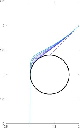
Figure 5: Artificial root not in breakdown configuration whose goal is to growth in depth

Simulation 1 In the first simulation the obstacle is a disc with center $(a,b)=(1.4,1)$ and radius $r=0.3$. The root has origin in $(2,2)$ and initial shape $y=x$ for $1.4\leq x\leq 2$. We fix the bound on the curvature $\kappa_{0}=4$. As we can see in Fig 5, the root bends, avoid the obstacle and grows vertically downward.

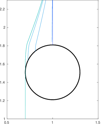
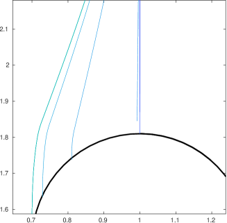
Figure 6: Artificial root in breakdown configuration which restarts

Simulation 2 Here we want to show how the restarting procedure works when the root is in a breakdown configuration. The obstacle is now a disc with center $(a^{\prime},b^{\prime})=(1,1.5)$ and radius $r=0.3$. The root has origin in $(1,2.5)$ and initial shape is $x=1$ for $1.8\leq y\leq 2.5$. The bound on the curvature is again $\kappa_{0}=4$. As we can see in Fig 6, the original root meets the obstacle perpendicularly with no curvature, hence by applying the restarting algorithm $(\ref{R1})$ the new attempt grows far from the previous one. In this way we can avoid the region already explored.

Compared with the simulations performed in [5], the main difference here is that the evolution of our curve is now described by two different equations, one for the body and one with the control for the tip. Thus, the procedure for adding nodes is different, since it is also determined by the feedback control.
Furthermore the robotic root must be able to recoil and restart whenever needed. This requires to take into account all previous attempts, in order not to travel close to trajectories already investigated. For simplicity, in the above simulations we have neglected the additional function $h$, describing the hardness of the soil. This corresponds to the case where the root descends into an empty cavity, between rigid obstacles.

Acknowledgments. The authors would like to thank Prof. Piero Marcati for suggesting the problem. The first author was partially supported by the Istituto Nazionale di Alta Matematica “F. Severi", through GNAMPA. The research of the second and third authors was partially supported by NSF, with grant DMS-1714237 “Models of controlled biological growth".

References

• [1] F. Ancona, A. Bressan, O. Glass, and W. Shen, Feedback stabilization of stem growth, Journal of Dynamics and Differential Equations, (2017), pp. 1–28.
• [2] N. Bessonov and V. Volpert, On a model of plant growth, in Patterns and waves (Saint Petersburg, 2002), AkademPrint, St. Petersburg, 2003, pp. 323–337.
• [3] N. Bessonov and V. Volpert, Dynamic models of plant growth, Mathematics and Mathematical Modelling, Publibook, Paris, 2006.
• [4] A. Bressan and M. Palladino, Well-posedness of a model for the growth of tree stems and vines, Discrete Contin. Dyn. Syst., 38 (2018), pp. 2047–2064.
• [5] A. Bressan, M. Palladino, and W. Shen, Growth models for tree stems and vines, J. Differential Equations, 263 (2017), pp. 2280–2316.
• [6] J. Burgner-Kahrs, D. C. Rucker, and H. Choset, Continuum robots for medical applications: A survey, IEEE Transactions on Robotics, VOLUME = 31, YEAR = 2015, NUMBER = 6, PAGES = 1261–1280,.
• [7] G. Dal Maso, An introduction to $\Gamma$-convergence, vol. 8 of Progress in Nonlinear Differential Equations and their Applications, Birkhäuser Boston, Inc., Boston, MA, 1993.
• [8] G. Dal Maso, A. DeSimone, and M. G. Mora, Quasistatic evolution problems for linearly elastic-perfectly plastic materials, Arch. Ration. Mech. Anal., 180 (2006), pp. 237–291.
• [9] A. R. Dexter, Mechanics of root growth, Plant and Soil, 98 (1987), pp. 303–312.
• [10] A. Goriely, The Mathematics and Mechanics of Biological Growth, Springer, 2017.
• [11] J. D. Greer, L. H. Blumenschein, A. M. Okamura, and E. W. Hawkes, Obstacle-aided navigation of a soft growing robot, in 2018 IEEE International Conference on Robotics and Automation (ICRA), May 2018, pp. 1–8.
• [12] J. D. Greer, T. K. Morimoto, A. M. Okamura, and E. W. Hawkes, A soft, steerable continuum robot that grows via tip extension, Soft Robotics, 6 (2019), pp. 95–108. PMID: 30339050.
• [13] O. Leyser and S. Day, Mechanisms in Plant Development, Blackwell Publishing, 2003.
• [14] A. Mainik and A. Mielke, Existence results for energetic models for rate-independent systems, Calc. Var. Partial Differential Equations, 22 (2005), pp. 73–99.
• [15] R. Pfeifer, M. Lungarella, and F. Iida, Self-organization, embodiment, and biologically inspired robotics, Science, 318 (2007), p. 1088Ð1093.
• [16] A. Sadeghi, A. Mondini, and B. Mazzolai, Toward self-growing soft robots inspired by plant roots and based on additive manufacturing technologies, Soft robotics, 4 (2017), pp. 211–223.
• [17] A. Sadeghi, A. Tonazzini, L. Popova, and B. Mazzolai, A novel growing device inspired by plant root soil penetration behaviors, PLOS ONE, 9 (2014), pp. 1–10.
• [18] I. D. Walker, Robot strings: Long, thin continuum robots, in 2013 IEEE Aerospace Conference, March 2013, pp. 1–12.
• [19] M. B. Wooten and I. D. Walker, Vine-inspired continuum tendril robots and circumnutations, Robotics, 7 (2018).