Numerical computation of periodic orbits and isochrons for state-dependent delay perturbation of an ODE in the plane

Abstract.

We present algorithms and their implementation to compute limit cycles and their isochrons for state-dependent delay equations (SDDE’s) which are perturbed from a planar differential equation with a limit cycle.

Note that the space of solutions of an SDDE is infinite dimensional. We compute a two parameter family of solutions of the SDDE which converge to the solutions of the ODE as the perturbation goes to zero in a neighborhood of the limit cycle.

The method we use formulates functional equations among periodic functions (or functions converging exponentially to periodic). The functional equations express that the functions solve the SDDE. Therefore, rather than evolving initial data and finding solutions of a certain shape, we consider spaces of functions with the desired shape and require that they are solutions.

The mathematical theory of these invariance equations is developed in a companion paper, which develops a posteriori theorems. They show that, if there is a sufficiently approximate solution (with respect to some explicit condition numbers), then there is a true solution close to the approximate one. Since the numerical methods produce an approximate solution, and provide estimates of the condition numbers, we can make sure that the numerical solutions we consider approximate true solutions.

In this paper, we choose a systematic way to approximate functions by a finite set of numbers (Taylor-Fourier series) and develop a toolkit of algorithms that implement the operators – notably composition – that enter into the theory. We also present several implementation results and present the results of running the algorithms and their implementation in some representative cases.

1. Introduction

Many phenomena in nature and technology are described by limit cycles and by now there is an extensive mathematical theory of them [Min62, AVK87].

These limit cycles often arise in feedback loops between effects that pump and remove energy in ways that depend on the state of the system. When the feedback happens instantaneously, these phenomena are modeled by an ordinary differential equation (ODE). Nevertheless, in many real phenomena, the feedback takes time to start acting. In such cases, the appropriate models are delay differential equations (DDE’s) in which the time derivative of a state is given by an expression which involves the state at a previous time. Such delays are documented to be important in several areas of science and technology (e.g. in electrodynamics, population dynamics, neuroscience, circuits, manufacturing, etc. See [HKWW06] for a relatively recent survey documenting many areas where DDE’s are important models).

Note that, from the mathematical point of view, adding even a small delay term in the ODE model is a very singular perturbation since the nature of the problem changes drastically. Notably, the natural phase spaces in delay equations are infinite dimensional (there is some discussions about what are the most natural ones) rather than the finite dimensional phase spaces of ODE.

One would heuristically expect that, if the delay term is a small quantity, there are solutions of the delay problem that resemble the solutions of the unperturbed ODE. Due to the singular perturbation nature of the problem, justifying this intuitive idea is a nontrivial mathematical task. Of course, besides the finite dimensional set of solutions that resemble the solutions of the ODE, one expects many other solutions, which may be very different. [HKWW06].

The recent rigorous paper [YGdlL20], describes a formalism to study the effect of introducing a delay to an equation in the plane with a limit cycle. The paper [YGdlL20] shows that, in some appropriate sense, the solutions of the ordinary differential equation persist. The method in [YGdlL20] is constructive since it is based on showing that the iterations of an explicit operator converge.

The goal of this paper is to present algorithms and implementation details for the mathematical arguments developed in [YGdlL20]. One also expects that solutions we compute – and which resemble the solutions of the ODE – capture the full dynamics of the SDDE in the sense that the solutions of the SDDE in a neighborhood converge to this finite dimensional solution family very fast.

The algorithms consist in specifying discretizations for all the functional analysis steps in [YGdlL20]. We do not present rigorous estimates on the effects of discretizations (they are in principle applications of standard estimates), but we present analysis of running times. We have implemented the algorithms above and report the results of running them in some representative examples. In our examples, one can indeed obtain very accurate solutions in a few minutes in a standard today’s laptop. Thanks to the a posteriori theorems in [YGdlL20], we can guarantee that these solutions correspond to true solutions of the problem.

We recall that the method of [YGdlL20] consists in bypassing the evolution and formulating the existence of periodic orbits (and the solutions converging to them) as the solutions in a class of functions with periodicity. Furthermore, the paper [YGdlL20] establishes an a posteriori theorem which states that given a sufficiently approximate solution of the invariance equation, there is a true solution close to it. To be more precise, an approximate solution is sufficiently approximate, if the error is smaller than an explicit expression involving several properties of the approximate solution (commonly called condition numbers).

The numerical methods developed and run here, produce an approximate solution and obtain estimates on the condition numbers. So, we can be quite confident that the solutions produced by our numerical methods correspond to true solutions.

Remark 1.1.

Although the results in [YGdlL20] have been detailed for the case of SDDE’s, they also apply without major modifications to advanced or even mixed differential equations.

Remark 1.2.

The paper [YGdlL20] includes a theory for different regularities of the differential equation, but in this numerical paper, we will only formulate results for analytic systems. Since we will specify which derivatives appear in the calculations, it is clear that the algorithms apply also for problems with finite differentiability.

Remark 1.3.

One of the consequences of the approach in [YGdlL20] is that one can easily obtain smooth dependence on parameters for the solutions. Note that if one studies the periodic orbits as fixed points of an evolution operator, one needs to study the smooth dependence of the solutions on the initial data and on parameters, which is a delicate question for general solutions. See [HVL93, Chapter 3.7].

Remark 1.4.

The a posteriori results justify that the approximate solution is independent of the method for which it has been produced.

Besides the numerical approximations, it is also customary in applied mathematics to produce approximate solutions using formal asymptotic expansions. For the problem at hand, the paper [CCdlL19] develops formal asymptotic expansions of the periodic solutions in powers of the term in the delay.

The expansions in [CCdlL19] are readily computable with the methods presented here. They can be taken as starting points for the fixed point method in [YGdlL20]. Moreover, the a posteriori results of [YGdlL20] show that these expansions are asymptotic in a very strong sense.

Remark 1.5.

The paper [YGdlL20] also includes some local uniqueness statements of the solutions (under the condition that the solutions have a certain shape). Hence the numerically computed approximate solutions of the invariance equation identify a unique solution, which is unambiguous. This uniqueness is crucial to compare different numerical runs as well as to obtain smooth dependence on parameters.

The uniqueness in [YGdlL20] is somewhat subtle. The limit cycle is unique as well as the Taylor expansions of isochrons (their parameterizations are unique once we fix origins of coordinates and scales). On the other hand, the full isochrons are unique only when one specifies a cut-off. Similar effects happen in the study of center manifolds [Sij85].

From the numerical point of view, we only compute the limit cycle and a finite Taylor expansion of the isochrons. The error of the reminder of the Taylor expansion is indeed very small (much smaller than other sources of numerical error, which are already small).

1.1. Organization of the paper

The paper is organized in an increasing level of details trying to guide the reader from the general steps of the algorithms to the more specialized and hardest steps of them.

First of all, we detail in section §2 an overview of the method developed in [YGdlL20]. In particular, we first introduce the situation of the unperturbed problem in §2.1 in order to move to the perturbed problem in §2.2. This will lead to the explicit expression of the invariance equation in §2.3 and the periodicity and normalization conditions in §2.6 and §2.7.

Our results start from the unperturbed case in [HdlL13], we will summarize in §3 the steps and add practical comments for numerically computing a parameterization in the unperturbed case.

The algorithms that allow to solve the invariance equation introduced in §2.3 are fully detailed in section §4.

The numerical composition of periodic mappings as well as its computational complexity needs special care. Hence, section §5 explains in detail such a process in a Fourier representation.

Finally, section §6 reports the results of some numerical experiments.

2. Overview of the problem and the method

2.1. The parameterization method for limit cycles and their isochrons in ODE’s

Our starting point is the main result in [HdlL13], which we recall informally (omitting precisions on regularity, domains of definition, etc).

Given an analytic ordinary differential equation (ODE) in the plane

$$\dot{x}=X_{0}(x)$$ (1)

with a (stable) limit cycle, there is an analytic local diffeomorphism $K$, in particular a local change of variables, defined from $\mathbb{T}\times[-1,1]$ to $\mathbb{R}^{2}$, a frequency $\omega_{0}>0$ and a rate $\lambda_{0}<0$ such that

$$X_{0}\circ K(\theta,s)=(\omega_{0}\partial_{\theta}+\lambda_{0}s\partial_{s})K(\theta,s)=DK(\theta,s)\begin{pmatrix}\omega_{0}\\ \lambda_{0}s\end{pmatrix}.$$ (2)

Hence, if $\theta$ and $s$ satisfy the very simple ODE

$$\begin{split}&\dot{\theta}(t)=\omega_{0},\\ &\dot{s}(t)=\lambda_{0}s(t),\end{split}$$ (3)

then

$$x(t)=K(\theta(t),s(t))$$

is a solution of (1) in a neighborhood of the limit cycle.

Therefore, the paper [HdlL13] trades finding all the solutions near the limit cycle of (1) for finding, $K$, $\omega_{0}$ and $\lambda_{0}$ solving (2). The paper [HdlL13] also develops efficient algorithms for the study of (2), the so-called invariance equation.

The key idea of the formalism in [YGdlL20] consists in accommodating the delay by just changing the equation (2). We will obtain a modified functional equation, which involves non-local terms that reflect the delay in time. This equation was treated in [YGdlL20]. Hence, we will produce a two dimensional family of solutions of the delay problem which resemble the solutions of the unperturbed problem (1).

The solutions we construct are analogues for the SDDE of the limit cycle as well as the solutions that converge to the limit cycle exponentially fast (notice that for the simple ODE, these are all the solutions with initial data in a neighborhood of the limit cycle).

The set $I_{\theta_{0}}=\{K(\theta_{0},s_{0})\colon s_{0}\in[-1,1]\}$ is called in the biology literature the “isochron” of $\theta_{0}$ because the orbit of a point in $I_{\theta_{0}}$ converges to the limit cycle with a phase $\theta_{0}$. See [Win75].

Remark 2.1.

The theory of normally hyperbolic manifolds shows that the isochrons are the same as the stable manifolds of points [Guc75] (see also [CL04] for generalizations beyond normal hyperbolicity).

Therefore, in the ODE case, isochrons and stable manifolds can be used interchangeably. In the SDDE case, however, the stable manifolds are infinite dimensional objects. The solutions we construct are finite dimensional families. To avoid confusion with the stable manifolds in [HVL93], we prefer to maintain the name isochrons to refer to the solutions we construct. Thus, the isochrons we constuct are subsets of the (infinite dimennsional) manifolds constructed in [HVL93]. As a matter of fact, they are slow manifolds, they correspond to the least stable eigenvalues. One expects that, in applications, the isochrons will be the most observable solutions since they correspond to the modes that decrease the slowest so that any solution will converge to the isochron much faster than the isochron converges to the limit cycle (an analogue with what happens in ODE in a stable node).

2.2. The perturbed problem

We consider now a perturbation of (1) of the form

$$\begin{split}\dot{x}(t)=&X\bigl{(}x(t),\varepsilon x(t-r(x))\bigr{)}\\ \coloneq&X(x(t),0)+\varepsilon P(x(t),x(t-r(x)),\varepsilon)\end{split}$$ (4)

where $0<\varepsilon\ll 1$, $X(x(t),0)=X_{0}(x(t))$ and $\varepsilon P(x(t),x(t-r(x)),\varepsilon)\coloneq X\bigl{(}x(t),\varepsilon x(t-r(x))\bigr{)}-X(x(t),0)$ and the function $r$ is positive and as smooth as we need, hence bounded in compact sets.

The equation (4) is a state-dependent delay differential equation (SDDE) for $\varepsilon\neq 0$. For typographical reasons we will denote $\widetilde{x}(t)\coloneq x(t-r(x))$.

2.3. The invariance equation in the perturbed problem

Let $\tilde{\mathbb{T}}$ be the universal cover of the 1-dimensional torus $\mathbb{T}$ and let us consider $K\colon\tilde{\mathbb{T}}\times[-1,1]\rightarrow\mathbb{R}^{2}$, the frequency as $\omega_{0}$ and the rate as $\lambda_{0}$ which solve (2). They correspond to the case $\varepsilon=0$ in (4).

In analogy with the ODE case, we want to find a $W(\theta,s)$ with periodicity in the first variable and numbers $\omega$ and $\lambda$ such that for all $\theta$ and $s$,

$$x(t)=K\circ W(\theta+\omega t,se^{\lambda t})$$ (5)

is a solution of (4).

The mapping $W$ gives us a parameterization of the limit cycle with its isochrons via $K\circ W(\theta,s)$. That is, the limit cycle will be represented by the set $\{K\circ W(\theta,0)\colon\theta\in\mathbb{T}\}$ and the isochron associated to the angle $\theta$ in $\mathbb{T}$ will be $\{K\circ W(\theta,s)\colon s\in[-s_{0},s_{0}]\}$ where $s_{0}$ denotes a region of validity in $s$ in the solution (5).

Note that, heuristically (and it is also shown in [YGdlL20]) $W$ is close to the identity map and $\omega$ and $\lambda$ are close to the values in the unperturbed case. Hence, we will produce a two-dimensional family of solutions of the delayed equation (4) which resemble the solutions of the ODE.

Remark 2.2.

Since the phase space of the delay equation is infinite dimensional, we expect that there are many more solutions of (4).

Based on the theory of [HVL93, Chapter 10], we know that the periodic orbit in the phase space of the SDDE is locally unique, hence the solution we produce has to agree with the periodic solution produced in [HVL93, Theorem 4.1].

The theory of delay equations [HVL93, Chapter 10] (specially Theorem 3.2) produces stable (or strong stable) manifolds in the (infinite dimensional) phase space. The stable manifolds produced in [HVL93] are infinite dimensional. Note that, since the evolution operators are compact, most of the eigenvalues of the evolution are very small, in particular, smaller than the $\lambda$ we will select later, so that the solutions in the stable manifold converge to the space of solutions produced here in a very fast way.

Imposing that the tuple $(W,\omega,\lambda)$ is such that (5) is a solution of (4) and knowing that the tuple $(K,\omega_{0},\lambda_{0})$ is also a solution of (2) but for $\varepsilon=0$, then

$$DK\circ WDW=DK\circ W\begin{pmatrix}\omega_{0}\\ \lambda_{0}W_{2}\end{pmatrix}+\varepsilon P(K\circ W,K\circ\widetilde{W},\varepsilon),$$ (6)

where $W_{2}$ refers to the second component of $W$.

Now, since $K$ is a local diffeomorphism, it also acts as a change of variable. In particular, we can premultiply (6) by $(DK\circ W)^{-1}$ to get the functional equation, whose unknowns are $W\equiv(W_{1},W_{2})$, $\omega$ and $\lambda$. That functional equation will be called invariance equation,

$$(\omega\partial_{\theta}+\lambda s\partial_{s})W(\theta,s)=\begin{pmatrix}\omega_{0}\\ \lambda_{0}W_{2}(\theta,s)\end{pmatrix}+\varepsilon Y\bigl{(}W(\theta,s),\widetilde{W}(\theta,s),\varepsilon\bigr{)},$$ (7)

where we use the shorthand

$$\begin{split}\widetilde{W}(\theta,s)&\coloneq W\bigl{(}\theta-\omega r(K\circ W),se^{-\lambda r(K\circ W)}\bigr{)},\\ Y\bigl{(}W(\theta,s),\widetilde{W}(\theta,s),\varepsilon\bigr{)}&\coloneq(DK\circ W(\theta,s))^{-1}P\bigl{(}K\circ W(\theta,s),K\circ\widetilde{W}(\theta,s),\varepsilon\bigr{)}.\end{split}$$

The equation (7) will be the center of our attention. Let us start by making some preliminary remarks on it.

We have ignored the precise definition of the domain of the function $W$. We need the range of $W$ to be contained in the domain of $K$. Note also that it is not clear that the domain of the RHS can match the domain of the LHS of (7). As it turns out, this will not matter much for our treatment providing a small enough $\varepsilon$ (see [YGdlL20] for a detailed discussion).

The equation (7) is underdetermined. That means, if $W,\omega$ and $\lambda$ solve equation (7), then $W_{\sigma,\eta},\omega$ and $\lambda$ also solve the same equation with

$$W_{\sigma,\eta}(\theta,s)=W(\theta+\sigma,\eta s).$$ (8)

The parameter $\sigma$ and $\eta$ correspond respectively to choosing a different origin in the angle coordinate $\theta$ and a different scale of the parameter $s$.

Even if all these solutions in (8) are mathematically equivalent, we anticipate that choosing a different $\eta$ can change the reliability of the numerical algorithms.

In [YGdlL20], it is shown that the solutions in the family (8) are locally unique. That is, all the solutions of the invariance equation (7) are included in (8). In equations (12) and (13) we introduce normalization conditions that specify the parameters in (8). This is useful for numerics since it allows to compare easily solutions obtained in different runs with different discretization sizes.

Remark 2.3.

From the point of view of analysis, one of the main difficulties of the equation (7) is that it involves a function composed with itself (hence the operator is not really differentiable). Also the term $\widetilde{W}$ does not have the same domain as $W$. We refer to [YGdlL20] for a deeper discussion in the composition domain.

Similar problems appear in the treatment of center manifolds [LI73, Car81] and indeed, in [YGdlL20] there are only results for finite differentiable solutions and the solutions obtained may depend on cut-offs and extensions taken to solve the problem.

Based on the experience with center manifolds, we believe that indeed, the solutions could only be finitely differentiable and that there are different solutions of the invariance equation (depending on the extensions considered).

Remark 2.4.

In the language of ergodic theory, for those familiar with it, the results of [YGdlL20] can be described as saying that there is a factor in the (infinite dimensional) phase space of the SDDE which is a two dimensional flow with dynamics close to the dynamics of the ODE.

In this paper, we will compute numerical approximations of the map giving the semiconjugacy as well as the new dynamics of such a factor.

2.4. Format of solution for the invariance equation (7)

It is shown in [YGdlL20] that, for small $\varepsilon$, one can construct smooth solutions of (7) of the form

$$W(\theta,s)=W^{0}(\theta)+W^{1}(\theta)s+\sum_{j=2}^{n}W^{j}(\theta)s^{j}+W^{>}(\theta,s)$$ (9)

where $W^{j}\colon\mathbb{T}\rightarrow\mathbb{T}\times\mathbb{R}$ and $W^{>}\colon\mathbb{T}\times[-s_{0},s_{0}]\rightarrow\mathbb{T}\times\mathbb{R}$ with $W^{>}(\theta,s)=O(s^{n+1})$ and for some $s_{0}>0$.

As we will see in more detail later on, if one substitutes (9) into (7) and matches powers in $s$, one gets a finite set of recursive equations for the coefficients $W^{j}$ of the expansion (and for $\omega$, $\lambda$). We will deal with these equations in detail later. Note that this will require a discretization of $W^{j}$, which are only functions of the angle $\theta$.

2.5. The equations for terms of the expansion of $W$

Assume for the moment that $W^{0}$ and $W^{1}$ have already been computed. Then we can substitute the expansion (9) of $W$ in powers of $s$ into the invariance equation (7). Matching the coefficients of the powers of $s$ on both sides we obtain a hierarchy of equations for $W^{j}$, $j=2,3,\ldots$.

The equations for $W^{j}$ involve just $W^{0},\dotsc,W^{j-1}$. Hence, they can be studied recursively. In [YGdlL20] it is shown that, if we know $W^{0},\dotsc,W^{j-1}$, it is possible to find $W^{j}$ in a unique way and, hence, we can proceed to solve the equations recursively. In this paper, we show that there are precise algorithms to compute these recursions. We also report results of implementation in some cases.

Note that $W^{j}$, $j=0,\ldots,n$ in (9) are functions only of $\theta$. The function $W^{>}$ depends both on $\theta$ and $s$ but vanishes at high order in $s$ and does not enter in the equations for $j=0,\dotsc,n$.

As it frequently happens in perturbative expansions, the low order equations are special. The equation for $W^{0}$ – which gives the periodic solution that continues the limit cycle – also determines $\omega$. The equation for $W^{1}$ also determines $\lambda$. The equations for $W^{j}$, $j=2,\dotsc,n$ are all similar and involve solving the same operator (with different terms).

In this paper, we will only consider the computation of the $W^{j}$, $j=0,1,\ldots$. The term $W^{>}$, is estimated in [YGdlL20] and it is not only high order in $s$ but also actually small in rather large balls.

Note that even if the $W^{j}$ are unique (up to the parameters in (8)), the $W^{>}$ depends on properties of the extension considered. This is, of course very reminiscent of what happens in the theory of center manifolds [Sij85] . For numerical studies of expansions of center manifolds we refer to [BK98, Jor99, PR06] and detailed estimates of the truncation in [CR12]. The numerical considerations about the effect of the truncation apply with minor changes to our case.

2.6. Periodicity conditions

From the point of view of implementation in computers, it is convenient to think of the functions $K$ and $W$ in (7) which involve angle variables (and which range on angles), as real functions with boundary conditions (in mathematical language this is described as taking lifts). Hence, we take

$$\begin{split}K(\theta+1,s)&=K(\theta,s),\\ W(\theta+1,s)&=W(\theta,s)+\begin{pmatrix}1\\ 0\end{pmatrix}.\end{split}$$ (10)

Notice that we are normalizing the angles to run between $0$ and $1$. Very often, the angles are taken to run in $[0,2\pi)$.

The periodicity conditions in (10) indicate the second component of $W$ is periodic (it describes a radial coordinate) in $\theta$ while the first component increases by $1$ when $\theta$ increases by $1$ (it describes an angle). So that the circle described by increasing $\theta$ makes the angle in the coordinate go around, so that it is a non-contractible circle in the angle.

For the expansion of $W$ in powers of $s$ as in (9), the periodicity conditions amount to:

$$W^{0}(\theta+1)=W^{0}(\theta)+\begin{pmatrix}1\\ 0\end{pmatrix}\quad\text{and}\quad W^{j}(\theta+1)=W^{j}(\theta)\quad\text{for }j\geq 1.$$ (11)

In the numerical analysis, there are many well-known ways to discretize periodic functions. We will use Fourier series, but there are also other alternatives such as periodic splines.

In general, for functions $\Psi$ with $\Psi(\theta+1)=\Psi(\theta)+1$, we define ${\widetilde{\Psi}}(\theta)=\Psi(\theta)-\theta$ which is a periodic function, i.e. for all $\theta$, ${\widetilde{\Psi}}(\theta+1)={\widetilde{\Psi}}(\theta)$. Then we will discretize $\widetilde{\Psi}$ and rewrite the functional equations so that this is the only unknown.

2.7. Normalization of the solutions

As indicated in the discussion, the invariance equation has two obvious sources of indeterminacy: One is the choice of the origin of the variable $\theta$ (the $\sigma$ in (8)) and the other is the choice of the scale of the variable $s$ (the $\eta$ in (8)) . In [YGdlL20] it is shown that these are the only indeterminacies and that once we fix them, we can get any other solution by applying (8).

A convenient way to fix the origin of $\theta$ is to require

$$\int_{0}^{1}\bigl{[}\partial_{\theta}W^{0}_{1}(\theta,0)\,W_{1}(\theta,0)\bigr{]}\,d\theta=a$$ (12)

where $W^{0}$ is an initial approximation and $a$ is a real number, typically it is closed to $1$. This normalization is easy to compute and is rather sensitive since, when we move in the family (8), the derivative with respect to the shift is a positive number.

The normalization of the origin of coordinates, has no numerical consequences except for the possibility of comparing the solutions in different runs. The solutions corresponding to different normalizations have very similar properties. The numerical algorithm 4.1 in its step 5 leads to a small drift in the normalization in each iteration, but it is guaranteed to converge to one of the solutions in (8).

The second normalization is just a choice of the eigenvector of an operator. We have found it convenient to take

$$\int_{0}^{1}\partial_{s}W_{2}(\theta,0)\,d\theta=\rho$$ (13)

with a real $\rho\neq 0$.

We anticipate that changing the value of $\rho$ is equivalent to changing $s$ into $bs$ where $b$ is commonly named scaling factor.

All the choices of $\rho$ are mathematically equivalent – they amount to setting the scale of the parameter $s$ –. The choice of this normalization, however, affects the numerical accuracy dramatically. Notice that if we change $s$ into $bs$, the coefficients $W^{j}(\theta)$ in (9) change into $W^{j}(\theta)b^{j}$. So, different choices of $b$ may lead the Taylor coefficients to be very large or very small, which makes the computations with them very susceptible to round off error. It is numerically advantageous to choose the scale in such a way that the Taylor coefficients have a comparable size.

In practice, we run the calculations twice. A preliminary one whose only purpose is to compute an approximation of the scale that makes the coefficients to remain more or less of the same size. Then, a more definitive calculation can be run. That last running is more numerically reliable.

Remark 2.5.

In standard implementation of the Newton Method for fixed points of a functional, say $\Psi$, the fact that the space of solutions is two dimensional leads $D\Psi-\text{Id}$ to have a two dimensional kernel, and not being invertible.

In our case, we will develop a very explicit and fast algorithm that produces an approximate linear right inverse. This linear right inverse leads to convergence to an element of the family (8).

3. Computation of $(K,\omega_{0},\lambda_{0})$ – unperturbed case

For completeness, we quote the Algorithm 4.4 in [HdlL13] adding some practical comments. That algorithm allows us to numerically compute $\omega_{0}$, $\lambda_{0}$ and $K\colon\tilde{\mathbb{T}}\times[-1,1]\rightarrow\mathbb{R}^{2}$ in (7). We note that the algorithm has quadratic convergence as it was proved in [HdlL13].

Algorithm 3.1.

Quasi-Newton method

1. Input: $\dot{x}=X(x)$ in $\mathbb{R}^{2}$, $K(\theta,s)=K^{0}(\theta)+K^{1}(\theta)b_{0}s$, $\omega_{0}>0$, $\lambda_{0}\in\mathbb{R}$ and scaling factor $b_{0}>0$.

2. Output: $K(\theta,s)=\sum_{j=0}^{m-1}K^{j}(\theta)(b_{0}s)^{j}$, $\omega_{0}$ and $\lambda_{0}$ such that $\lVert E\rVert\ll 1$.

3. $E\leftarrow X\circ K-(\omega_{0}\partial_{\theta}+\lambda_{0}s\partial_{s})K$.

4. Solve $DK\tilde{E}=E$ and denote $\tilde{E}\equiv(\tilde{E}_{1},\tilde{E}_{2})$.

5. $\sigma\leftarrow\int_{0}^{1}\tilde{E}_{1}(\theta,0)\,d\theta$ and $\eta\leftarrow\int_{0}^{1}\partial_{s}\tilde{E}_{2}(\theta,0)\,d\theta$.

6. $E_{1}\leftarrow\tilde{E}_{1}-\sigma$ and $E_{2}\leftarrow\tilde{E}_{2}-\eta s$.

7. Solve $(\omega_{0}\partial_{\theta}+\lambda_{0}s\partial_{s})S_{1}=E_{1}$ imposing

   $$\int_{0}^{1}S_{1}(\theta,0)\,d\theta=0.$$ (14)

8. Solve $(\omega_{0}\partial_{\theta}+\lambda_{0}s\partial_{s})S_{2}-\lambda_{0}S_{2}=E_{2}$ imposing

   $$\int_{0}^{1}\partial_{s}S_{2}(\theta,0)\,d\theta=0.$$ (15)

9. $S\equiv(S_{1},S_{2})$.

10. Update: $K\leftarrow K+DKS$, $\omega_{0}\leftarrow\omega_{0}+\sigma$ and $\lambda_{0}\leftarrow\lambda_{0}+\eta$.

11. Iterate (1) until convergence in $K$, $\omega$ and $\lambda$. Then undo the scaling $b_{0}$.

Algorithm 3.1 requires some practical considerations:

1. It is clear that the most delicate steps of above algorithm are 5 and 6, which are often called cohomology equations. These steps involve solving PDE’s whereas the others are much simpler. Indeed, the discretizations used are dictated by the desire of solving these equations in an efficient way.

2. Initial guess. $K^{0}\colon\tilde{\mathbb{T}}\rightarrow\mathbb{R}^{2}$ will be a parameterization of the periodic orbit of the ODE with frequency $\omega_{0}$. It can be obtained, for instance, by a Poincaré section method, continuation of integrable systems or Lindstedt series. An approximation for $K^{1}\colon\tilde{\mathbb{T}}\rightarrow\mathbb{R}^{2}$ and $\lambda$ can be obtained by solving the variational equation

   $$DX\circ K^{0}(\theta)U(\theta) =\omega_{0}\frac{d}{d\theta}U(\theta),$$

   $$U(0) =Id_{2}.$$

   Hence if $(e^{\lambda_{0}/\omega_{0}},K^{1}(0))$ is the eigenpair of $U(1)$ such that $\lambda_{0}<0$, then $K^{1}(\theta)=U(\theta)K^{1}(0)e^{-\lambda_{0}\theta/\omega_{0}}$.

3. Stopping criteria. As any Newton method, a possible condition to stop the iteration can be when either $\lVert E\rVert$ or $\max\{\lVert DKS\rVert,\lvert\sigma\rvert,\lvert\eta\rvert\}$ is smaller than a given tolerance.

   Note that the a posteriori theorems in [HdlL13] give a criterion of smallness on the error depending on properties of the function $K$. If these criteria are satisfied, one can ensure that there is a true solution close to the numerical one.

4. Uniqueness. Note that in the steps 5 and 6, which involve solving the cohomology equations, the solutions are determined only up to adding constants in the zero or first order terms. We have adopted the conventions (14), (15). These conventions make the solution operator linear (which matches well the standard theory of Nash-Moser methods since it is easy to estimate the norm of the solutions).

   As it is shown in [HdlL13], the algorithm converges quadratically fast to a solution, but since the problem is underdetermined, we have to be careful when comparing solutions of different discretization. In [HdlL13] there is discussion of the uniqueness, but for our purposes in this paper, any of the solutions will work. The uniqueness of the solutions considered in this paper is discussed in section §2.7.

5. Convergence. It has been proved in [HdlL13] that even of the quasi-Newton method, it still has quadratic convergence.

   Note that it is remarkable that we can implement a Newton like method without having to store – much less invert – any large matrix. Note also that we can get a Newton method even if the derivative of the operator in the fixed point equation has eigenvalues $1$. See remark 2.5.

3.1. Fourier discretization of periodic functions

As it was mentioned before, the key step of Algorithm 3.1 is to solve the equations in steps 5 and 6. Their numerical resolution will be particularly efficient when the functions are discretized in Fourier-Taylor series. This will be the only discretization we will consider in this paper providing a deep discussion.

Remark 3.2.

Even if we will not use it in this paper, we remark that [HdlL13, §4.3.1] there are two methods to solve them. One assumes a Fourier representation in terms of the angle $\theta$ and the other uses integral expressions which can be evaluated efficiently in several discretizations of the functions (e.g. splines). The spline representation could be preferable to the Fourier-Taylor in some regimes where the limit cycles are bursting.

Recall that a function $S\colon\mathbb{R}\rightarrow\mathbb{R}$ is called periodic when $S(\theta+1)=S(\theta)$ for all $\theta$.

To get a computer representation of a periodic function, we can either take a mesh in $\theta$, i.e. $(\theta_{k})_{k=0}^{n_{\theta}-1}$ and store the values of $S$ at these points: $\widecheck{S}=(\widecheck{S}_{k})_{k=0}^{n_{\theta}-1}\in\mathbb{R}^{n_{\theta}}$ with $\widecheck{S}_{k}=S(\theta_{k})$ or we can take advantage of the periodicity and represent it in a trigonometric basis.

The Discrete Fourier Transform (DFT), and also its inverse, allows to switch between the two representations above. If we fix a mesh of points of size $n_{\theta}$ uniformly distributed in $[0,1)$, i.e. $\theta_{k}=k/n_{\theta}$, the DFT is:

$$\widehat{S}=(\widehat{S}_{k})_{k=0}^{n_{\theta}-1}\in\mathbb{C}^{n_{\theta}}$$

so that

$$\widecheck{S}_{k}=\sum_{j=0}^{n_{\theta}-1}\widehat{S}_{j}e^{2\pi\boldsymbol{i}jk/n_{\theta}}$$ (16)

or equivalently

$$\widehat{S}_{k}=\frac{1}{n_{\theta}}\sum_{j=0}^{n_{\theta}-1}\widecheck{S}_{j}e^{-2\pi\boldsymbol{i}jk/n_{\theta}}.$$ (17)

In the case of a real valued function, $\widehat{S}_{0}$ is real and the complex numbers $\widehat{S}$ satisfy Hermitian symmetry, i.e. $\widehat{S}_{k}=\widehat{S}_{n_{\theta}-k}^{\ast}$ (denoting by ^∗ the complex conjugate), which implies $\widehat{S}_{n_{\theta}/2}$ real when $n_{\theta}$ is even. Then, we define real numbers $(a_{0};a_{k},b_{k})_{k=1}^{\lceil n_{\theta}/2\rceil-1}$ if $n_{\theta}$ is odd, here $\lceil\cdot\rceil$ denotes the ceil function, otherwise $(a_{0},a_{n_{\theta}/2};a_{k},b_{k})_{k=1}^{n_{\theta}/2-1}$ defined by

$$a_{0}=2\widehat{S}_{0}\text{, }a_{n_{\theta}/2}=2\widehat{S}_{n_{\theta}/2}\text{, }a_{k}=2\operatorname{Re}\widehat{S}_{k}\text{ and }b_{k}=-2\operatorname{Im}\widehat{S}_{k}$$

with $1\leq k<\lceil n_{\theta}/2\rceil$.

Thus, $S$ can be approximated by

$$S(\theta)=\frac{a_{0}}{2}+\frac{a_{n_{\theta}/2}}{2}\cos(\pi n_{\theta}\theta)+\sum_{k=1}^{\lceil n_{\theta}/2\rceil-1}a_{k}\cos(2\pi k\theta)+b_{k}\sin(2\pi k\theta)$$ (18)

where the coefficient $a_{n_{\theta}/2}$ only appears when $n_{\theta}$ is even and it refers to the aliasing notion in signal theory.

Therefore (18) is equivalent to (16) but rather than $2n_{\theta}$ real numbers, only half of them are needed.

Henceforth, all real periodic functions $S$ can be represented in a computer by an array of length $n_{\theta}$ whose values are either the values of $S$ on a grid or the Fourier coefficients. These two representations are, for all practical purposes equivalent since there is a well known algorithm, Fast Fourier Transform (FFT), which allows to go from one to the other in $\Theta(n_{\theta}\log n_{\theta})$ operations. The FFT has very efficient implementations so that the theoretical estimates on time are realistic (we can use fftw3 [FJ05], which optimizes the use of the hardware).

We can also think of functions of two variables $W(\theta,s)$ where one variable $\theta$ is periodic and the other variable $s$ is a real variable. In the numerical implementations, the variable $s$ will be discretized as a polynomial. Thus $W(\theta,s)$ can be thought as a function of $\theta$ taking values in polynomials of length $n_{s}$. Hence, a function of two variables with periodicity as above will be discretized by an array $n_{\theta}\times n_{s}$. The meaning could be that it is a polynomial for each value of $\theta$ in a mesh or that it a polynomial of whose coefficients are Fourier coefficients. Alternatively, we could think of $W(\theta,s)$ as a polynomial in $s$ taking values in a space of periodic functions.

This mixed representation of Fourier series in one variable and power series in another variable, is often called Fourier-Taylor series and has been used in celestial mechanics for a long time, dates back to [BG69] or earlier. We note that, modern computer languages allow to overload the arithmetic operations among different types in a simple way.

It is important to note that all the operations in Algorithm 3.1 are fast either on the Fourier representation or in the values of a mesh representation. For example, the product of two functions or the composition on the left with a known function are fast in the representation by values in a mesh. More importantly for us, as we will see, the solution of cohomology equations is fast in the Fourier representation. On the other hand, there are other steps of Algorithm 3.1, such as adding, are fast in both representations.

Similar consideration of the efficiency of the steps will apply to the algorithms needed to solve our problem. The main novelty of the algorithms in this paper compared with those of [HdlL13] is that we will need to compose some of the unknown functions (in [HdlL13] the unknowns are only composed on the left with a known function). The algorithms we use to deal with composition will be presented in section §5. The composition operator will be the most delicate numerical aspect, which was to be expected, since it was also the most delicate step in the analysis in [YGdlL20]. The composition operator is analytically subtle. A study which gives examples that results are sharp is in [dlLO99]. See also [AZ90].

Remark 3.3.

Fourier series are extremely efficient for smooth functions which do not have very pronounced spikes. For rather smooth functions – a situation that appears often in practice – it seems that Fourier Taylor series is better than other methods.

It should be noted, however that in several models of interest in electronics and neuroscience, the solutions move slowly during a large fraction of the period, but there is a fast movement for a short time (bursting). In these situations, the Fourier scheme has the disadvantage that the coefficients decrease slowly and that the discretization method does not allow to put more effort in describing the solutions during the times that they are indeed changing fast. Hence, the Fourier methods become unpractical when the limit cycles are bursting. In such cases, one can use other methods of discretization. In this paper, we will not discuss alternative numerical methods, but note that the theoretical estimates of [YGdlL20] remain valid independent of the method of discretization. We hope to come back to implementing the toolkit of operations of this paper in other discretizations.

Remark 3.4.

One of the confusing practical aspects of the actual implementation is that the coefficients of the Fourier arrays are often stored in a complicated order to optimize the operations and the access during the FFT.

For example concerning the coefficients $a_{k}$’s and $b_{k}$’s in (18), in fftw3, the fftw_plan_r2r_1d uses the following order of the Fourier coefficients in a real array $(v_{0},\dotsc,v_{n_{\theta}-1})$.

$$v_{0} =a_{0},$$

$$v_{k} =2a_{k}\text{ and }v_{n_{\theta}-k}=-2b_{k}\quad\text{ for }1\leq k<\lceil n_{\theta}/2\rceil,$$

$$v_{n_{\theta}/2} =a_{n_{\theta}/2}$$

where the index $n_{\theta}/2$ is taken into consideration if and only if $n_{\theta}$ is even. Another standard order in other packages is just $(a_{0},a_{n_{\theta}/2};a_{k},b_{k})$ in sequential order or $(a_{0};a_{k},b_{k})$ if $n_{\theta}$ is odd.

To measure errors and size of functions represented by Fourier series, we have found useful to deal with weighted norms involving the Fourier coefficients.

$$\lVert S\rVert_{w\ell^{1},n} =2(n_{\theta}/2)^{n}|\widehat{S}_{n_{\theta}/2}|+\sum_{k=1}^{\lceil n_{\theta}/2\rceil-1}((n_{\theta}-k)^{n}+k^{n})\lvert\widehat{S}_{k}\rvert$$

$$=(n_{\theta}/2)^{n}\lvert a_{n_{\theta}/2}\rvert+\frac{1}{2}\sum_{k=1}^{\lceil n_{\theta}/2\rceil-1}((n_{\theta}-k)^{n}+k^{n})(a_{k}^{2}+b_{k}^{2})^{1/2}.$$

where, again, the term for $n_{\theta}/2$ only appears if $n_{\theta}$ is even.

The smoothness of $S$ can be measured by the speed of decay of the Fourier coefficients and indeed, the above norms give useful regularity classes that have been studied by harmonic analysts.

Remark 3.5.

The relation of the above regularity classes with the the most common $C^{m}$ is not straightforward, as it is well known by Harmonic analysts, [Ste70].

Riemann-Lebesgue’s Lemma tells us that if $S$ is continuous and periodic, $\widehat{S}_{k}\to 0$ as $k\to\infty$ and in general if $S$ is $m$ times differentiable, then $\lvert\widehat{S}_{k}\rvert|k|^{m}$ tends to zero. In particular, $\lvert\widehat{S}_{k}\rvert\leq C/\lvert k\rvert^{m}$ for some constant $C>0$.

In the other direction, from $\lvert\widehat{S}_{k}\rvert\leq C/\lvert k\rvert^{m}$ we cannot deduce that $S\in C^{m}$.

One has to use more complicated methods. In [dlLP02] it was found that one could find a practical method based on Littlewood-Paley theorem (see [Ste70]) which states that the function $S$ is in $\alpha$-Hölder space with $\alpha\in\mathbb{R}_{+}$ if and only if, for each $\eta\geq 0$ there is constant $C>0$ such that for all $t>0$.

$$\biggl{\lVert}\biggl{(}\frac{\partial}{\partial t}\biggr{)}^{\eta}e^{-t\sqrt{-\Delta}\theta}\biggr{\rVert}_{L^{\infty}(\mathbb{T})}\leq Ct^{\alpha-\eta}.$$

The above formula is easy to implement if one has the Fourier coefficients, as it is the case in our algorithms.

3.2. Solutions of the cohomology equations in Fourier representation

Under the Fourier representation we can solve the cohomological equations in the steps 5 and 6 of the Algorithm 3.1.

Proposition 3.6 (Fourier version, [HdlL13]).

Let $E(\theta,s)=\sum_{j,k}E_{jk}e^{2\pi\boldsymbol{i}k\theta}s^{j}$.

• If $E_{00}=0$, then $(\omega\partial_{\theta}+\lambda s\partial_{s})u(\theta,s)=E(\theta,s)$ has solution $u(\theta,s)=\sum_{j,k}u_{jk}e^{2\pi\boldsymbol{i}k\theta}s^{j}$ and

  $$u_{jk}=\begin{cases}\frac{E_{jk}}{\lambda j+2\pi\boldsymbol{i}\omega k}&\text{if }(j,k)\neq(0,0)\\ \alpha&\text{otherwise}.\end{cases}$$

  for all real $\alpha$. Imposing $\int_{0}^{1}u(\theta,0)\,d\theta=0$, then $\alpha=0$.

• If $E_{10}=0$, then $(\omega\partial_{\theta}+\lambda s\partial_{s}-\lambda)u(\theta,s)=E(\theta,s)$ has solution $u(\theta,s)=\sum_{j,k}u_{jk}e^{2\pi\boldsymbol{i}k\theta}s^{j}$ and

  $$u_{jk}=\begin{cases}\frac{E_{jk}}{\lambda(j-1)+2\pi\boldsymbol{i}\omega k}&\text{if }(j,k)\neq(1,0)\\ \alpha&\text{otherwise}.\end{cases}$$

  for all real $\alpha$. Imposing $\int_{0}^{1}\partial_{s}u(\theta,0)\,d\theta=0$, then $\alpha=0$.

The paper [HdlL13] also presents a solution in terms of integrals. Those integral formulas for the solution are independent of the discretization and work for discretizations such as Fourier series, splines and collocations methods. Indeed, the integral formulas are very efficient for discretizations in splines or in collocation methods. In this paper we will not use them since we will discretize functions in Fourier series and for this discretization, the methods described in Proposition 3.6 are more efficient.

3.3. Treatment of the step 2 in Algorithm 3.1

To solve the linear system in the step 2 of Algorithm 3.1, we can use Lemma 3.7, whose proof is a direct power matching.

Lemma 3.7.

Consider the equation for $x$ given by Let $A(\theta,s)x(\theta,s)=b(\theta,s)$ where $A,b$ are given. More explicitly:

$$\biggl{(}\sum_{k\geq 0}A_{k}(\theta)s^{k}\biggr{)}\sum_{k\geq 0}\boldsymbol{x}_{k}(\theta)s^{k}=\sum_{k\geq 0}\boldsymbol{b}_{k}(\theta)s^{k}.$$

Then, the coefficients $\boldsymbol{x}_{k}(\theta)$ are obtained recursively by solving

$$A_{0}(\theta)\boldsymbol{x}_{k}(\theta)=\boldsymbol{b}_{k}(\theta)-\sum_{j=1}^{k}A_{j}(\theta)\boldsymbol{x}_{k-j}(\theta).$$

which can be done provided that $A_{0}(\theta)$ is invertible and that one knows how to multiply and add periodic functions of $\theta$.

We also recall that composition of a polynomial in the left with a exponential, trigonometric functions, powers, logarithms (or any function that satisfies an easy differential equation) can be done very efficiently using algorithms that are reviewed in [HCF⁺16] which goes back to [Knu81].

We present here the case of the exponential which will be used later on in Algorithm 4.2.

If $P$ is a given polynomial – or a power series – with coefficients $P_{j}$, we see that $E(s)=\exp P(s)$ satisfies

$$\frac{d}{ds}E(s)=E(s)\frac{d}{ds}P(s)$$

Equating like powers on both sides, it leads to $E_{0}=\exp P(0)$, and the recursion:

$$E_{j}=\frac{1}{j}\sum_{k=0}^{j-1}(j-k)P_{j-k}E_{k}\text{, }\qquad j\geq 1,$$

Note that this can also be done if the coefficients of $P$ are periodic functions of $\theta$ (or polynomials in other variables). In modern languages supporting overloading or arithmetic functions, all this can be done in an automatic manner.

Note that if the polynomial has degree $n_{s}$, the computation up to degree $n_{s}$ takes $\Theta(n_{s}^{2})$ operations of multiplications of the coefficients.

4. Computation of $(W,\omega,\lambda)$ – perturbed case

The main result in the paper [YGdlL20] states that if $\varepsilon$ in (7) is small enough, a periodicity condition like (12) and a normalization like (13) are considered, then there exists a unique tuple $(W,\omega,\lambda)$ verifying (7), (12) and (13).

The formulation of that result in [YGdlL20] is done in a posteriori format which ensures the existence of a true solution once an approximate enough solution is provided as initial guess for the iterative scheme.

Moreover, it also gives the Lipschitz dependence of the solution on parameters which allows to consider a continuation approach.

We refer to [YGdlL20] for a precise formulation of the result involving choices of norms to measure the error in the approximate solutions.

4.1. Fixed point approach

We compute all the coefficients $W^{j}(\theta)$ of the truncated expression $W(\theta,s)$ in (9) order by order. The zero and first orders require a special attention due to the fact that the values $\omega$ and $\lambda$ are obtained in the equation (7) matching coefficients of $s^{0}$ and $s^{1}$ respectively. The condition that allows to obtain $\omega$ comes from the periodicity condition (11). The mapping $W^{0}$ is not a periodic function. But we can use it to get a periodic one defined by $\hat{W}^{0}(\theta)\coloneq W^{0}(\theta)-\left(\begin{smallmatrix}\theta\\ 0\end{smallmatrix}\right)$. The condition for $\lambda$ is given by the normalization condition (13). As in the unperturbed case, we are allowed to use a scaling factor. The use of such a scaling factor allows to set the value of $\rho$ in (13) equal to $1$.

Algorithm 4.1 sketches the fixed-point procedure to get $\omega$ and $W^{0}$ whose periodicity condition is ensured in step (5). In this case the initial condition will be $\omega_{0}$ (the value for $\varepsilon=0$) for $\omega$ and $\left(\begin{smallmatrix}\theta\\ 0\end{smallmatrix}\right)$ for $W^{0}(\theta)$ since $W(\theta,s)$ is close to the identity.

Algorithm 4.1 ($s^{0}$ case).

Let $\widetilde{W^{0}}(\theta)\coloneq W^{0}\bigl{(}\theta-\omega r\circ K(W^{0}(\theta))\bigr{)}$.

1. Input: $\dot{x}=X(x)+\varepsilon P(x,\tilde{x},\varepsilon)$, $0<\varepsilon\ll 1$, $K(\theta,s)=\sum_{j=0}^{m-1}K^{j}(\theta)(b_{0}s)^{j}$, $b_{0}>0$, $\omega_{0}>0$ and $\lambda_{0}<0$.

2. Output: $\hat{W}^{0}\colon\mathbb{T}\rightarrow\mathbb{R}^{2}$ and $\omega>0$.

3. $\hat{W}^{0}(\theta)\leftarrow 0$ and $\omega\leftarrow\omega_{0}$.

4. $W^{0}(\theta)\leftarrow\begin{pmatrix}\theta\\ 0\end{pmatrix}+\hat{W}^{0}(\theta)$.

5. Solve $DK\circ W^{0}(\theta)\eta(\theta)=\varepsilon P(K\circ W^{0}(\theta),K\circ\widetilde{W^{0}}(\theta),\varepsilon)$. Let $\eta\equiv(\eta_{1},\eta_{2})$.

6. $\alpha\leftarrow\int_{0}^{1}\eta_{1}(\theta)\,d\theta$ and $\omega\leftarrow\omega_{0}+\alpha$.

7. Solve $\omega\partial_{\theta}\hat{W}_{1}^{0}(\theta)=\eta_{1}(\theta)-\alpha$ imposing $\int_{0}^{1}\hat{W}_{1}^{0}(\theta)\,d\theta=0$.

8. Solve $(\omega\partial_{\theta}-\lambda_{0})\hat{W}_{2}^{0}(\theta)=\eta_{2}(\theta)$.

9. Iterate (2) until convergence in $W^{0}$ and $\omega$.

Algorithm 4.2 sketches the steps to compute $(W^{1},\lambda)$ and $W^{n}$ for $n\geq 2$. The initial guesses are $\lambda_{0}$ for $\lambda$, $\left(\begin{smallmatrix}0\\ 1\end{smallmatrix}\right)$ for $W^{1}$ and $\left(\begin{smallmatrix}0\\ 0\end{smallmatrix}\right)$ for $W^{n}$. In either case, it is required to solve a linear system of the form of Lemma 3.7 as well as cohomological equation similar to the unperturbed case.

Algorithm 4.2 ($s^{1}$ case and $s^{n}$ case with $n\geq 2$).

Let $\widetilde{W}(\theta,s)\coloneq W\bigl{(}\theta-\omega r\circ K(W(\theta,s)),se^{-\lambda r\circ K(W(\theta,s))}\bigr{)}$.

1. Input: $\dot{x}=X(x)+\varepsilon P(x,\widetilde{x},\varepsilon)$, $0<\varepsilon\ll 1$, $K(\theta,s)=\sum_{j=0}^{m-1}K^{j}(\theta)(b_{0}s)^{j}$, $b_{0}>0$, $\omega_{0}>0$, $\lambda_{0}<0$, $\hat{W}^{0}(\theta)$, $W^{j}(\theta)$ for $0<j<n$, $b>0$ and $\omega>0$.

2. Output: either $W^{1}\colon\mathbb{T}\rightarrow\mathbb{T}\times\mathbb{R}$ and $\lambda<0$ or $W^{n}\colon\mathbb{T}\rightarrow\mathbb{T}\times\mathbb{R}$.

3. $W^{n}(\theta)\leftarrow\begin{pmatrix}0\\ 0\end{pmatrix}$.

4. If $n=1$, $W^{1}(\theta)\leftarrow\begin{pmatrix}0\\ 1\end{pmatrix}$ and $\lambda\leftarrow\lambda_{0}$.

5. $W(\theta,s)\leftarrow\begin{pmatrix}\theta\\ 0\end{pmatrix}+\hat{W}^{0}(\theta)+\sum\limits_{j=1}^{n}W^{j}(\theta)(bs)^{j}$.

6. $Y(W(\theta,s))\leftarrow DK\circ W(\theta,s)^{-1}P(K\circ W(\theta,s),K\circ\widetilde{W}(\theta,s),\varepsilon)$.

7. $\eta(\theta)\leftarrow\varepsilon\frac{\partial^{n}Y}{\partial s^{n}}(W(\theta,s))_{|s=0}$. Let $\eta\equiv(\eta_{1},\eta_{2})$.

8. If $n=1$, then $\lambda\leftarrow\lambda_{0}+\int_{0}^{1}\eta_{2}(\theta)\,d\theta$.

9. Solve $(\omega\partial_{\theta}+n\lambda)W_{1}^{n}(\theta)=\eta_{1}(\theta)$.

10. Solve $(\omega\partial_{\theta}+n\lambda-\lambda_{0})W_{2}^{n}(\theta)=\eta_{2}(\theta)$.

11. Iterate (2) until convergence. Then undo the scaling $b$.

Both algorithms 4.1 and 4.2 have non-trivial parts, such as, the effective computation of $\widetilde{W}$, the numerical composition of $K$ with $W$ and also with $\widetilde{W}$ (see §5), the effective computation of the step 4 in Algorithm 4.2, the stopping criterion (see §4.1.1) and the choice of the scaling factor (see §4.1.2). On the other hand, there are steps that we can use the same methods in the unperturbed case, such as, the solution of linear systems like step 3 in Algorithm 4.2 via Lemma 3.7 or the solutions of the cohomological equations via Proposition 3.6.

4.1.1. Stopping criterion

algorithms 4.1 and 4.2 require to stop the iterations when prescribed tolerances have been reached. Alternatively, one can stop when the invariance equation is satisfied up to a given tolerance.

4.1.2. Scaling factor

As in the unperturbed case, if $W(\theta,s)$ is a solution, then $W(\theta+\theta_{0},bs)$ will be a solution too for any $\theta_{0}$ and $b$. A difference with the $\varepsilon=0$ case is that now $K\circ W$ and $K\circ\widetilde{W}$ are required to be well-defined. That means the second components of $W$ and $\widetilde{W}$ must lie in $[-1,1]$. Stronger conditions are

$$p(s)=\sum_{j\geq 0}\lVert W_{2}^{j}(\theta)\rVert\lvert s\rvert^{j}\leq 1\qquad\text{and}\qquad\widetilde{p}(s)=\sum_{j\geq 0}\lVert\widetilde{W_{2}^{j}}(\theta)\rVert\lvert s\rvert^{j}\leq 1.$$

In the iterative scheme of Algorithm 4.2, these series become finite sums and a condition for the value $b>0$ is led by the upper-bound $\min\{s^{\ast},\widetilde{s}^{\ast}\}$ where $s^{\ast}$ is the value so that $p(s^{\ast})=1$ and, similarly, $\widetilde{s}^{*}$ the value verifying $\widetilde{p}(\widetilde{s}^{\ast})=1$. Notice that, the solutions $s^{\ast}$ and $\widetilde{s}^{\ast}$ exist because $\lVert W_{2}^{0}(\theta)\rVert<1$, $\lVert\widetilde{W_{2}^{0}}(\theta)\rVert<1$ and the polynomials are strictly positive for $s\geq 0$.

5. Numerical composition of periodic maps

The goal of this section is to deeply discuss how we can numerically compute $\widetilde{W}$, the compositions $K\circ W(\theta,s)$ and $K\circ\widetilde{W}(\theta,s)$ only having a numerical representation (or approximation) of $K$ and $W$ in the algorithms 4.1 and 4.2.

There are a variety of methods that can be employed to numerically get the composition of a periodic mapping with another (or the same) mapping. Some of these methods depend strongly on the representation of the periodic mapping and others only depend on specific parts of the algorithm.

We start the discussion from the general methods to those that strongly depend on the numerical representation. One expects that the general ones will have a bigger numerical complexity or it will be less accurate.

Before starting to discuss the algorithms, it is important to stress again that for functions of two variables $(\theta,s)\in\mathbb{T}\times[-1,1]$, there are two complementary ways of looking at them. We can think of them as functions that given $\theta$ produce a polynomial in $s$ – this polynomial valued function will be periodic in $\theta$ – or we can think of them as polynomials in $s$ taking values in spaces of periodic functions (of the variable $\theta$). Of course, the periodic functions that appear in our interpretation can be discretized either by the values in a grid of points or by the Fourier transform.

Each of these – equivalent! – interpretations will be useful in some algorithms. In the second interpretation, we can “overload” algorithms for standard polynomials to work with polynomials whose coefficients are periodic functions (in particular Horner schemes). In the first interpretation, we can easily parallelize algorithms for polynomials for each of the values of $\theta$ using the grid discretization of periodic functions.

Possibly the hardest part of algorithms 4.1 and 4.2 is the compositions between $K$ with $W$ and with $\widetilde{W}$. Due to the step 4 of Algorithm 4.2 the composition should be done so that the output is still a polynomial in $s$ with coefficients that are periodic functions of $\theta$.

In our implementation, we use the Automatic Differentiation (AD) approach [HCF⁺16, GW08].

If $W(\theta,s)=(W_{1}(\theta,s),W_{2}(\theta,s))$ is a function of two variables taking values in $\mathbb{R}^{2}$, then

$$K\circ W(\theta,s)=\sum_{j=0}^{m-1}K^{j}(W_{1}(\theta,s)))\left(b_{0}W_{2}(\theta,s)\right)^{j},$$ (19)

which can be evaluated with $m-1$ polynomial products and $m-1$ polynomial sums using Horner scheme, once we have computed $K^{j}\circ W_{1}(\theta,s)$.

The problem of composing a periodic function with a periodic polynomial in $s$ – to produce a polynomial in $s$ taking values in the space of periodic functions – is what we consider now.

The most general method considers $S$ a periodic function, the $K^{j}$ in (19), and $q(s)=\sum_{j=0}^{k}q_{j}s^{j}$ a polynomial of a fixed order $k\geq 0$ where the $q_{j}$ are periodic functions of $\theta$ that we consider discretized by their values in a grid.

We want to compute the polynomial $p\coloneq S\circ q$ up to order $k$. Assume that $\frac{d^{j}}{d\theta^{j}}S(q_{0})$ for $0\leq j\leq k$ are given as input and that they have been previously computed in a bounded computational cost. The chain rule gives us a procedure to compute the coefficients of $p(s)=\sum_{j=0}^{k}p_{j}s^{j}$.

Indeed, one can build a table, whose entries are polynomials in $s$, like in Table 1 following the generation rule in Figure 1.

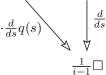
Figure 1. Generation rule for $i=2,\dotsc,k+1$ Table 1 entries

The inputs of Table 1 are $a_{i,1}=0$ for $i\neq 1$ and $a_{2,2}=\frac{d}{ds}q(s)$. Then the entries $a_{ij}$ with $2\leq j\leq i\leq k+1$ are given by

$$a_{ij}(s)=\frac{1}{i-1}\left(\frac{d}{ds}a_{i-1,j}(s)+a_{i-1,j-1}(s)\frac{d}{ds}q(s)\right).$$ (20)

Thus, the coefficients of $p(s)$ are $p_{j}=\sum_{l=0}^{k}a_{jl}(0)\frac{d^{l}}{d\theta^{l}}S(q_{0})$ for $0\leq j\leq k$.

$$\begin{array}[]{l||*{6}{c}}&S(q_{0})&\frac{d}{d\theta}S(q_{0})&\frac{d^{2}}{d\theta^{2}}S(q_{0})&\cdots&\frac{d^{k-1}}{d\theta^{k-1}}S(q_{0})&\frac{d^{k}}{d\theta^{k}}S(q_{0})\\ \hline\cr\hline\cr p_{0}&1&0\\ p_{1}&0&\frac{d}{ds}q(s)&0\\ p_{2}&0&\frac{1}{2}\square&\frac{1}{2}\square\\ \vdots&\vdots&\vdots&\vdots&\ddots&0\\ p_{k-1}&0&\frac{1}{k-1}\square&\frac{1}{k-1}\square&\cdots&\frac{1}{k-1}\square&0\\ p_{k}&0&\frac{1}{k}\square&\frac{1}{k}\square&\cdots&\frac{1}{k}\square&\frac{1}{k}\square\\ \end{array}$$

Table 1. Composition of a function with a polynomial

Note that it is enough to store in memory $k$ entries of the Table 1 to compute all the coefficients $p_{j}$.

Moreover, for each entry in the $i$th row with $i=2,\dotsc,k+1$, one only needs to consider polynomials of degree $k+1-i$. Overall the memory required is at most $\frac{1}{2}k(k+1)$. The number of arithmetic operations following the rule (20) are given by the Proposition 5.1.

Proposition 5.1.

Let $S$ be a real-periodic function and let $q(s)$ be a real polynomial of degree $k$. Given $\frac{d^{j}}{d\theta^{j}}S(q(0))$ for $j=0,\dotsc,k$. The polynomial $S\circ q$ can be performed using Table 1 with $\frac{1}{2}k(k+1)$ units of memory and $\Theta(k^{4})$ multiplications and additions.

Proof.

Note that $k(k+1)$ multiplications and $(k+1)^{2}$ additions are needed to perform the product of two polynomials of degree $k$. Also $k$ multiplications are needed to perform the derivative of a polynomial of degree $k$ multiplied by a scalar. To bound the number of operations we must distinct three different situations of the Table 1.

1. The column $a_{3..k,2}$. $\sum\limits_{i=1}^{k-2}(k-i+1)=\frac{1}{2}(k^{2}+k-6)$ multiplications.

2. The diagonal $a_{3..k,3..k}$.

   • $\sum\limits_{j=1}^{k-2}(k-j-1)(k-j+1)+1=\frac{1}{6}(2k^{3}-3k^{2}+k-6)$ multiplications.

   • $\sum\limits_{j=1}^{k-2}(k-j-1)^{2}+1=\frac{1}{6}(2k^{3}-9k^{2}+19k-18)$ additions.

3. The rest.

   • $\sum\limits_{j=1}^{k-2}\sum\limits_{i=j+1}^{k-2}(k-i-1)(k-i+1)+(k-i-2)+1=\frac{1}{12}(7k^{4}-56k^{3}+71k^{2}+38k-24)$ multiplications.

   • $\sum\limits_{j=1}^{k-2}\sum\limits_{i=j+1}^{k-2}(k-i-1)^{2}+(k-i)+1=\frac{1}{12}(5k^{4}-36k^{3}+85k^{2}-102k+72)$ additions.

Overall $\frac{7}{12}k^{4}+\Theta(k^{3})$ multiplications and $\frac{5}{12}k^{4}+\Theta(k^{3})$ additions. ∎

The next Theorem 5.2 summarizes the previous explanations and it provides the complexities to numerically compute $K\circ W$ in (19). It assumes that $\frac{d^{i}}{d\theta^{i}}S(q_{0})$ of Table 1 are given as input because their computation strongly depends on the numerical representation of a periodic mapping.

Theorem 5.2.

For a fixed $\theta$, the computational complexity to compute the compositions of $K(\theta,s)=\sum_{j=0}^{m-1}K^{j}(\theta)(b_{0}s)^{j}$ with $W(\theta,s)=\sum_{j=0}^{k-1}W^{j}(\theta)(bs)^{j}$ and $\widetilde{W}(\theta,s)$ using Table 1 is $\Theta(mk^{4})$ and space $\Omega(k^{2})$ assuming $\frac{d^{i}}{d\theta^{i}}K^{j}(W^{0}_{1}(\theta))$ as input for $i=0,\dotsc,k-1$.

Remark 5.3.

In general, if $n_{\theta}$ denotes the mesh size of the variable $\theta$, we will have $k\leq m\ll n_{\theta}$. That is, the mesh size will be much larger than the degree (in $s$) of $K(\theta,s)$. That means that the parallelization in $n_{\theta}$ will be more advantageous.

Theorem 5.2 has an important assumption involving $\frac{d^{i}}{d\theta^{i}}K^{j}(W_{1}^{0}(\theta))$ which can have a big impact in the complexity of $K\circ W(\theta,s)$. However, such an impact strongly depends on the numerical representation of $K^{j}$ and it will be discussed in the Fourier representation case.

5.1. Composition in Fourier

Theorem 5.2 reduces the problem of computing $K\circ W(\theta,s)$ in (19) to the problem of computing composition of a periodic function with another one. Such a composition of real Fourier truncated series may require to know the values not in the standard equispaced mesh of $\theta$ which hampers the use of the FFT. A direct composition of real Fourier series requires a computational complexity $\Theta(n_{\theta}^{2})$. However it can be performed with $\Theta(n_{\theta}\log n_{\theta})$ by the nfft3, see [KKP09]. The package nfft3 allows to express $S\colon\mathbb{T}\rightarrow\mathbb{R}$ with the same coefficients in (16) and perform its evaluation in an even number of non-equispaced nodes $(\theta_{k})_{k=0}^{n_{\theta}-1}\subset\mathbb{T}$ by

$$S(\theta_{k})=\sum_{j=0}^{n_{\theta}-1}\widehat{S}^{j}e^{-2\pi\boldsymbol{i}(j-n_{\theta}/2)(\theta_{k}-1/2)}.$$ (21)

The corrections of $\theta_{k}$ in (21) is because nfft3 considers $\mathbb{T}\simeq[-1/2,1/2)$ rather than the other standard equispaced discretization in $[0,1)$. nfft3 uses some window functions for a first approximation as a cut-off in the frequency domain and also for a second approximation as a cut-off in time domain. It takes under control (by bounds) these approximations to ensure the solution is a good approximation. Joining these result with Proposition 5.1 we can rewrite Theorem 5.2 as

Theorem 5.4.

The computational complexity to compute in Algorithm 4.2 the compositions of $K(\theta,s)=\sum_{j=0}^{m-1}K^{j}(\theta)(b_{0}s)^{j}$ with $W(\theta,s)=\sum_{j=0}^{k-1}W^{j}(\theta)(bs)^{j}$ and $\widetilde{W}(\theta,s)=\sum_{j=0}^{k-1}\widetilde{W}^{j}(\theta)(bs)^{j}$ using Table 1 and nfft3, and assuming that $K^{j}$, $W^{j}$ and $\widetilde{W}^{j}$ are expressed with $n_{\theta}$ Fourier coefficients is $\Theta(mk^{4}n_{\theta}+mkn_{\theta}\log n_{\theta})$. The space complexity is $\Omega(kn_{\theta}+k^{2})$.

Remark 5.5.

The remark 5.3 also applies to Theorem 5.4 in terms of the parallelization of $n_{\theta}$ due to the fact that in general $k\leq m\ll n_{\theta}$. However, in the parallelism case, the space complexity increase to $\Omega(kn_{\theta}+k^{2}n_{p})$ with $n_{p}$ the number of processes although the part corresponding to $kn_{\theta}$ can be shared memory.

In particular, the nfft3 can also be used for the zero order $W^{0}$ of Algorithm 4.1 giving in that case the same complexity as Theorem 5.4 but with $k=1$.

5.2. Automatic Differentiation in Fourier

Theorem 5.2 tells us that the composition $K\circ W(\theta,s)$ can numerically be done independently of the periodic mapping representation. Nevertheless, differentiation is a notoriously ill-posed problem due to the lack of information in the discretized problem. Thus, Table 1 is a good option when no advantage of the computer periodic representation exists or $k\ll m$.

Using the representation (18), we can use the Taylor expansion of the sine and cosine by recurrence [Knu81, HCF⁺16]. That is, if $q(s)$ is a polynomial, then $\sin q(s)$ and $\cos q(s)$ are given by $s_{0}=\sin q_{0}$, $c_{0}=\cos q_{0}$ and for $j\geq 1$,

$$s_{j}=\frac{1}{j}\sum_{k=0}^{j-1}(j-k)q_{j-k}c_{k},\qquad c_{j}=-\frac{1}{j}\sum_{k=0}^{j-1}(j-k)q_{j-k}s_{k}.$$ (22)

Therefore the computational cost to obtain the sine and cosine of a polynomial is linear with respect to its degree.

Theorem 5.6 says that the composition of $K$ with $W$ or $\widetilde{W}$ are rather than $\Theta(mk^{4}n_{\theta}+mkn_{\theta}\log n_{\theta})$ like in Theorem 5.4 just $\Theta(mkn_{\theta}^{2})$. Therefore if $k\ll m$ and $n_{\theta}$ is large, the approach given by Theorem 5.4 has a better complexity although Theorem 5.6 will be more stable for larger $k$.

Theorem 5.6.

The computational complexity to compute in Algorithm 4.2 the compositions of $K(\theta,s)=\sum_{j=0}^{m-1}K^{j}(\theta)(b_{0}s)^{j}$ with $W(\theta,s)=\sum_{j=0}^{k-1}W^{j}(\theta)(bs)^{j}$ and $\widetilde{W}(\theta,s)=\sum_{j=0}^{k-1}\widetilde{W}^{j}(\theta)(bs)^{j}$ using Automatic Differentiation and assuming that $K^{j}$, $W^{j}$ and $\widetilde{W}^{j}$ are expressed with $n_{\theta}$ Fourier coefficients is $\Theta(mkn_{\theta}^{2})$.

6. Numerical results

The van der Pol oscillator [vdP20] is an oscillator with a non-linear damping governed by a second-order differential equation.

The state-dependent perturbation of the van der Pol oscillator in [HG15] has the form

$$\begin{split}\dot{x}(t)&=y(t),\\ \dot{y}(t)&=\mu(1-x(t)^{2})y(t)-x(t)+\varepsilon x(t-r(x(t))),\end{split}$$ (23)

with $\mu>0$ and $0<\varepsilon\ll 1$. For the delay function $r(x)$ we are going to consider two cases. A pure state-dependent delay case $r(x)=0.006e^{2x}$ or just a constant delay case $r(x)=0.006$.

The first step consists in computing the change of coordinate $K$, the frequency $\omega_{0}$ of the limit cycle and its stability value $\lambda_{0}<0$ for $\varepsilon=0$. By standard methods of computing periodic orbits and their first variational equations, we compute the limit cycles close to $(x,y)=(2,0)$ for different values of $\mu$. Table 2 shows the values of $\omega_{0}$ and $\lambda_{0}$ for each of those values of the parameter $\mu$.

$$\begin{array}[]{l|c|c}\mu&\omega_{0}&\lambda_{0}\\ \hline\cr\hline\cr 0.25&\mathtt{0.1585366857025485}&\mathtt{-0.2509741760777654}\\ 0.5&\mathtt{0.1567232109993800}&\mathtt{-0.5077310891698608}\\ 1&\mathtt{0.1500760842377394}&\mathtt{-1.0593769948418550}\\ 1.5&\mathtt{0.1409170454968141}&\mathtt{-1.6837946490433340}\end{array}$$

Table 2. Values of $\omega_{0}$ and $\lambda_{0}$ for different values of the parameter $\mu$ in eq. (23) with $\varepsilon=0$

The computation of $K(\theta,s)$, following Algorithm 3.1, up to order $16$ in $s$ and with a Fourier mesh size of $1024$ allows to plot the isochrons in Figure 2.

In the case of ODE’s, the isochrons computed by evaluating the expansion can be globalized by integration of the ODE (23) forward and backward in time, see [HdlL13]. In the case of the SDDE, $\varepsilon\neq 0$, propagating backwards is not possible. We hope that this limitation can be overcome, but this will require some new rigorous developments and more algorithms. We think that this is a very interesting problem.

Figure 2. Limit cycles and their isochrons for different values of the parameter $\mu$ in the unperturbed, eq. (23)

A relevant indicator for engineers is the power spectrum, i.e. the square of the modulus of the complex Fourier coefficients. In Figure 3 we illustrate the power spectrum for $K^{0}$, since $K^{0}$ is the one that is commonly observed in a circuit system.

Figure 3. Logscale of the power spectrum of $K^{0}\equiv(K^{0}_{1},K^{0}_{2})$ for $\mu=1.5$ and $\varepsilon=0$ in eq. (23)

Due to the quadratic convergence of the Algorithm 3.1, see [HdlL13], the computation of Table 2 and Figure 2 are performed in less than one min in a today standard laptop. However, we notice that for values of $\mu>1.5$ the method may not converge for the unperturbed case, the scaling factor and the Fourier mesh size need to be smaller due to spikes, especially for the high orders in $s$, i.e. $K^{j}(\theta)$ for large $j$. This is an inherent drawback of the numerical representation of periodic functions that can be emphasized with the model involved.

6.1. Perturbed case

Let us analyze the case of $\mu=1.5$ for two different types of delay functions; a constant one $r(x)=0.006$ and a state-dependent one $r(x)=0.006e^{x}$.

The two cases have some advantages to be exploited. For instance, in the constant case $\widetilde{W}(\theta,s)=W(\theta-\omega\beta,se^{-\lambda\beta})$ is easier to compute than in the state-dependent case. Since in both cases $W$ and $\widetilde{W}$ must be composed by $K$, the use of automatic differentiation for the step 4 in Algorithm 4.2 is still needed. In particular, for the Algorithm 4.1 and the composition via Theorem 5.4, the nfft3 can be used to perform the numerical composition of $K$ with $W$ and $\widetilde{W}$.

The first steps of our method get $\omega$ and $\lambda$ which we distinguish their values depending on the delay function and the parameter $\varepsilon$. Again here we are assuming $\mu=1.5$. These values are summarized respectively in Tables 3 and 4. They were computed fixing a tolerance for the stopping criterion of $10^{-10}$ in double-precision. As one expects they are close to those in Table 2 and are further as $\varepsilon$ increase. Moreover we report a speed factor around $2.25$ using the nfft3 with respect to a direct implementation of the Fourier composition.

$$\begin{array}[]{c||c|c}\varepsilon&\omega_{s}&\omega_{c}\\ \hline\cr\hline\cr 10^{-4}&\mathtt{0.140908673246532}&\mathtt{0.140908547470887}\\ 10^{-3}&\mathtt{0.140833302396846}&\mathtt{0.140832045466042}\\ 10^{-2}&\mathtt{0.140077545298062}&\mathtt{0.140065058638519}\end{array}$$

Table 3. Values of $\omega$ for different values of $\varepsilon$ in eq. (23) with $\mu=1.5$ obtained by Algorithm 4.1. $\omega_{s}$ corresponds to the state-dependent delay and $\omega_{c}$ the constant delay

$$\begin{array}[]{c||c|c}\varepsilon&\lambda_{s}&\lambda_{c}\\ \hline\cr\hline\cr 10^{-4}&\mathtt{-1.6838123845562083}&\mathtt{-1.6838091880373793}\\ 10^{-3}&\mathtt{-1.6839721186835845}&\mathtt{-1.6839401491442914}\\ 10^{-2}&\mathtt{-1.6855808865357260}&\mathtt{-1.6852607528946115}\end{array}$$

Table 4. Values of $\lambda$ for different values of $\varepsilon$ in eq. (23) with $\mu=1.5$ obtained by Algorithm 4.2. $\lambda_{s}$ corresponds to the state-dependent delay and $\lambda_{c}$ the constant delay

Figure 4 shows, for different values of $\varepsilon$ in eq. (23), the logarithmic error of invariance equation for each of the different orders $j\geq 0$. That is, the finite system of invariance equations obtained after plugging $W(\theta,s)=\sum W^{j}(\theta)s^{j}$ into eq. (7) and matching terms of the same order. The state-dependent case needs smaller values of $\varepsilon$ to satisfy the invariance equation while the constant delay case admits larger values of $\varepsilon$ which can be deduced from the inequalities in [YGdlL20].

Figure 4. Log10 scale of the 2-norm of the error in the invariance equation

Figures 5 shows the difference between the isochrons for the perturbed and unperturbed case. As one expects from the theorems in [YGdlL20], the error is smaller as the perturbation parameter value $\varepsilon$ becomes smaller.

Figure 5. Log10 scale of the 2-norm of the difference between the perturbed and unperturbed cases. That is, $\lVert K^{j}-(K\circ W)^{j}\rVert$

An important point in Algorithm 4.2 is the well-definedness of the composition of $K$ with $W$ and $\widetilde{W}$. Because the state-dependent delays consider much more situations than just the constant delay, one expects that potentially smaller scaling factor compared to the constant delay will be needed as large order is computed. Figure 6 shows if $\varepsilon$ is far from the unperturbed case it will need to be smaller, that for the constant case is enough to use a constant scaling factor and for the state-dependent it decrease drastically in the first orders.

Figure 6. Scaling factor to ensure that the composition of $K$ with $W$ and with $\widetilde{W}$ in Algorithm 4.2 are well-defined

To illustrate the physical observation the Figures 7 and 8 shows the power spectra of the limit cycles after the perturbations. More concretely, Figure 7 displays the power spectrum of $(K\circ W)^{0}$ for the pure state-dependent delay case and $\varepsilon=0.01$. In contrast with Figure 3, we observe that for the even indexes they have non-zero values in the double-precision arithmetic sense. On the other hand, Figure 8 shows that these non-zero values in the even indexes are not present in the constant delay case and the power spectrum for the case $\varepsilon>0$ is away from that when $\varepsilon=0$ as $\varepsilon$ increase.

Figure 7. Log10 scale of the power spectrum of $(K\circ W)^{0}$ for $\mu=1.5$, $\varepsilon=0.01$ and the state-dependent delay $r(x)=0.006e^{x}$ in eq. (23)

Figure 8. Log10 scale of the difference between the power spectrum of $K^{0}$ and the power spectrum of $(K\circ W)^{0}$ for $\mu=1.5$, different values of $\varepsilon$ and constant delay $r=0.006$ in eq. (23)

References

- [AVK87] A. A. Andronov, A. A. Vitt, and S. È. Khaĭkin. Theory of oscillators. Dover Publications, Inc., New York, 1987. Translated from the Russian by F. Immirzi, Reprint of the 1966 translation.
- [AZ90] Jürgen Appell and Petr P. Zabrejko. Nonlinear superposition operators, volume 95 of Cambridge Tracts in Mathematics. Cambridge University Press, Cambridge, 1990.
- [BG69] R. Broucke and K. Garthwhite. A programming system for analytical series expansions on a computer. Celestial mechanics, 1(2):271–284, 1969.
- [BK98] Wolf-Jürgen Beyn and Winfried Kleß. Numerical Taylor expansions of invariant manifolds in large dynamical systems. Numer. Math., 80(1):1–38, 1998.
- [Car81] Jack Carr. Applications of centre manifold theory, volume 35 of Applied Mathematical Sciences. Springer-Verlag, New York-Berlin, 1981.
- [CCdlL19] Alfonso Casal, Livia Corsi, and Rafael de la Llave. Expansions in the delay of quasi-periodic solutions for state dependent delay equations. ArXiv, (1910.04808), 2019.
- [CL04] Carmen Chicone and Weishi Liu. Asymptotic phase revisited. J. Differential Equations, 204(1):227–246, 2004.
- [CR12] Maciej J. Capiński and Pablo Roldán. Existence of a center manifold in a practical domain around in the restricted three-body problem. SIAM J. Appl. Dyn. Syst., 11(1):285–318, 2012.
- [dlLO99] R. de la Llave and R. Obaya. Regularity of the composition operator in spaces of Hölder functions. Discrete Contin. Dynam. Systems, 5(1):157–184, 1999.
- [dlLP02] Rafael de la Llave and Nikola P. Petrov. Regularity of conjugacies between critical circle maps: an experimental study. Experiment. Math., 11(2):219–241, 2002.
- [FJ05] Matteo Frigo and Steven G. Johnson. The design and implementation of FFTW3. Proceedings of the IEEE, 93(2):216–231, 2005. Special issue on “Program Generation, Optimization, and Platform Adaptation”.
- [Guc75] J. Guckenheimer. Isochrons and phaseless sets. J. Math. Biol., 1(3):259–273, 1974/75.
- [GW08] Andreas Griewank and Andrea Walther. Evaluating derivatives. Society for Industrial and Applied Mathematics (SIAM), Philadelphia, PA, second edition, 2008. Principles and techniques of algorithmic differentiation.
- [HCF+16] Àlex Haro, Marta Canadell, Jordi-Lluís Figueras, Alejandro Luque, and Josep-Maria Mondelo. The parameterization method for invariant manifolds, volume 195 of Applied Mathematical Sciences. Springer, [Cham], 2016. From rigorous results to effective computations.
- [HdlL13] Gemma Huguet and Rafael de la Llave. Computation of limit cycles and their isochrons: fast algorithms and their convergence. SIAM J. Appl. Dyn. Syst., 12(4):1763–1802, 2013.
- [HG15] Aiyu Hou and Shangjiang Guo. Stability and Hopf bifurcation in van der Pol oscillators with state-dependent delayed feedback. Nonlinear Dynam., 79(4):2407–2419, 2015.
- [HKWW06] Ferenc Hartung, Tibor Krisztin, Hans-Otto Walther, and Jianhong Wu. Functional differential equations with state-dependent delays: theory and applications. In Handbook of differential equations: ordinary differential equations. Vol. III, Handb. Differ. Equ., pages 435–545. Elsevier/North-Holland, Amsterdam, 2006.
- [HVL93] Jack K. Hale and Sjoerd M. Verduyn Lunel. Introduction to functional-differential equations, volume 99 of Applied Mathematical Sciences. Springer-Verlag, New York, 1993.
- [Jor99] Àngel Jorba. A methodology for the numerical computation of normal forms, centre manifolds and first integrals of Hamiltonian systems. Experiment. Math., 8(2):155–195, 1999.
- [KKP09] Jens Keiner, Stefan Kunis, and Daniel Potts. Using NFFT 3—a software library for various nonequispaced fast Fourier transforms. ACM Trans. Math. Software, 36(4):Art. 19, 30, 2009.
- [Knu81] Donald E. Knuth. The art of computer programming. Vol. 2. Addison-Wesley Publishing Co., Reading, Mass., second edition, 1981. Seminumerical algorithms, Addison-Wesley Series in Computer Science and Information Processing.
- [LI73] Oscar E. Lanford III. Bifurcation of periodic solutions into invariant tori: the work of Ruelle and Takens. In Ivar Stakgold, Daniel D. Joseph, and David H. Sattinger, editors, Nonlinear problems in the Physical Sciences and biology: Proceedings of a Battelle summer institute, pages 159–192, Berlin, 1973. Springer-Verlag. Lecture Notes in Mathematics, Vol. 322.
- [Min62] Nicolas Minorsky. Nonlinear oscillations. D. Van Nostrand Co., Inc., Princeton, N.J.-Toronto-London-New York, 1962.
- [PR06] Christian Pötzsche and Martin Rasmussen. Taylor approximation of integral manifolds. J. Dynam. Differential Equations, 18(2):427–460, 2006.
- [Sij85] Jan Sijbrand. Properties of center manifolds. Trans. Amer. Math. Soc., 289(2):431–469, 1985.
- [Ste70] Elias M. Stein. Singular integrals and differentiability properties of functions. Princeton Mathematical Series, No. 30. Princeton University Press, Princeton, N.J., 1970.
- [vdP20] Balthasar van der Pol. A theory of the amplitude of free and forced triode vibrations. Radio Review., 1(701-710):754–762, 1920.
- [Win75] A. T. Winfree. Patterns of phase compromise in biological cycles. J. Math. Biol., 1(1):73–95, 1974/75.
- [YGdlL20] Jiaqi Yang, Joan Gimeno, and Rafael de la Llave. Parameterization method for state dependent delay perturbation of an ordinary differential equation. –, –(-):–, 2020.