Reconstruction of Multi-user Binary Subspace Chirps

Abstract

We consider codebooks of Complex Grassmannian Lines consisting of Binary Subspace Chirps (BSSCs) in $N=2^{m}$ dimensions. BSSCs are generalizations of Binary Chirps (BCs), their entries are either fourth-roots of unity, or zero. BSSCs consist of a BC in a non-zero subspace, described by an on-off pattern. Exploring the underlying binary symplectic geometry, we provide a unified framework for BSSC reconstruction—both on-off pattern and BC identification are related to stabilizer states of the underlying Heisenberg-Weyl algebra. In a multi-user random access scenario we show feasibility of reliable reconstruction of multiple simultaneously transmitted BSSCs with low complexity.

I Introduction

Codebooks of complex projective (Grassmann) lines, or tight frames, have applications in multiple problems of interest for communications and information processing, such as code division multiple access sequence design [1], precoding for multi-antenna transmissions [2] and network coding [3]. Contemporary interest in such codes arise, e.g., from deterministic compressed sensing [4, 5, 6, 7, 8], virtual full-duplex communication [9], mmWave communication [10], and random access [11]. In this paper, the main motivation will come from a random access scenario, in particular from a Massive Machine Type Communication (MTC) scenario [12], where the number of potentially accessing users may be extremely high, while a majority of devices may be stationary. In such scenarios, encoding and decoding complexity is of particular interest. To limit complexity and power consumption for MTC devices, it is important that a limited alphabet with small power variation is applied for transmission. Low decoding complexity is important for receiver implementation; complexity should not grow as a function of the number of codewords.

Codebooks of Binary Chirps (BCs) [5] provide an algebraically determined set of Grassmannian line codebooks in $N=2^{m}$ dimensions, with desirable properties; all entries are fourth root of unity and the minimum distance is $1/\sqrt{2}$. The number of codewords is reasonably large, growing as $2^{m(m+3)/2}$, while single-user decoding complexity is ${\cal O}(N\log^{2}N)$. Recently in [13], we expanded the set of Binary Chirps to Binary Subspace Chirps (BSSCs). Taking the underlying binary symplectic geometry fully into account, complex Grassmannian line codebooks are created with entries being either scaled fourth-roots of unity, or zero. Comparing to BCs, the minimum distance remains $1/\sqrt{2}$, the number of codewords is $\approx 2.38$ times larger, and a single-user decoder with complexity ${\cal O}(N\log^{3}N)$ is provided.

In this paper, we expand on [13]. Based on the underlying binary symplectic geometry, we provide a systematic way of looking at the reconstruction algorithm by making use of stabilizer states [14] and related notions in quantum computation. This combines the binary subspace reconstruction discussed in [13] and the BC reconstruction algorithm of [5] under the same algebraic framework. Furthermore, we investigate BSSC decoding in true random access scenarios, where there are multiple randomly selected users simultaneously accessing the channel. We provide a compressive sensing multi-user detection algorithm for $L$ simultaneously accessing randomly selected users with complexity ${\cal O}(N\log^{2+L}N)$. We find numerically that in a scenario where the channels of the randomly accessing users come from a continuous complex valued fading distribution, this multi-BSSC reconstruction algorithm is capable of reliable multi-user detection.

II Preliminaries

II-A The Binary Grassmannian ${\mathcal{G}}(m,r;2)$

A binary subspace $H\in{\mathcal{G}}(m,r;2)$ is the column space of some matrix ${\mathbf{H}}_{\mathcal{I}}$ in column reduced echelon form, where ${\mathcal{I}}\subset\{1,\ldots,m\}$ records the leading positions. The dual subspace of $H$ in ${\mathcal{G}}(m,m-r;2)$ is the column space of $\widetilde{{\mathbf{H}}_{\mathcal{I}}}$, with $({\mathbf{H}}_{{\mathcal{I}}})\mbox{${}^{\sf T}$}\widetilde{{\mathbf{H}}_{{\mathcal{I}}}}=0$. By ${\mathbf{I}}_{{\mathcal{I}}}$ we will denote the $m\times r$ consisting of the $r$ columns of the identity matrix indexed by ${\mathcal{I}}$. Put $\widetilde{{\mathcal{I}}}:=\{1,\ldots,m\}\setminus{\mathcal{I}}$. Then,

$$\begin{array}[]{ccc}({\mathbf{I}}_{{\mathcal{I}}})\mbox{${}^{\sf T}$}{\mathbf{H}}_{{\mathcal{I}}}={\mathbf{I}}_{r},&({\mathbf{I}}_{{\mathcal{I}}})\mbox{${}^{\sf T}$}{\mathbf{I}}_{\widetilde{{\mathcal{I}}}}=0,&\widetilde{{\mathbf{H}}_{{\mathcal{I}}}}{\mathbf{I}}_{\widetilde{{\mathcal{I}}}}={\mathbf{I}}_{m-r},\end{array}$$ (1)

and ${\mathbf{H}}_{{\mathcal{I}}}$ can be completed to an invertible matrix

$${\mathbf{P}}_{\scriptsize{\mathcal{I}}}:=\mbox{$\left[\!\!\begin{array}[]{cc}{{\mathbf{H}}_{{\mathcal{I}}}}&{{\mathbf{I}}_{\widetilde{{\mathcal{I}}}}}\end{array}\!\!\right]$}\in\mathrm{GL}(m;2).$$ (2)

The transposed inverse is given by

$${\mathbf{P}}_{\scriptsize{\mathcal{I}}}^{-\sf T}=\mbox{$\left[\!\!\begin{array}[]{cc}{{\mathbf{I}}_{{\mathcal{I}}}}&{\widetilde{{\mathbf{H}}_{{\mathcal{I}}}}}\end{array}\!\!\right]$}.$$ (3)

II-B Bruhat Decomposition of the Symplectic Group

We first briefly describe the symplectic structure of ${\mathbb{F}}_{2}^{2m}$ via the symplectic bilinear form

$$\mbox{$\langle{\,{{\mathbf{a}},{\bf b}}\,}|\,{{\mathbf{c}},{\mathbf{d}}}\,\rangle_{\rm s}$}:={\bf b}\mbox{${}^{\sf T}$}{\mathbf{c}}+{\mathbf{a}}\mbox{${}^{\sf T}$}{\mathbf{d}}.$$ (4)

A $2m\times 2m$ matrix ${\mathbf{F}}$ preserves $\langle{\,{\raisebox{0.86108pt}{\mbox{$\scriptscriptstyle\bullet\,$}}}\,}|\,{\raisebox{0.86108pt}{\mbox{$\scriptscriptstyle\bullet\,$}}}\,\rangle_{\rm s}$ iff ${\mathbf{F}}\mbox{\rm$\textbf{$\Omega$}$}{\mathbf{F}}\mbox{${}^{\sf T}$}=\mbox{\rm$\textbf{$\Omega$}$}$ where

$$\Omega=\mbox{$\left[\!\!\begin{array}[]{cc}{{\bf 0}_{m}}&{{\mathbf{I}}_{m}}\\ {{\mathbf{I}}_{m}}&{{\bf 0}_{m}}\end{array}\!\!\right]$}.$$ (5)

We will denote the group of all such symplectic matrices ${\mathbf{F}}$ with $\mathrm{Sp}(2m;2)$. To proceed, we use the Bruhat decomposition of $\mathrm{Sp}(2m;2)$ [15]. For ${\mathbf{P}}\in\mathrm{GL}(m;2)$ and ${\mathbf{S}}\in\mathrm{Sym}(m;2)$ we distinguish two types of elements in $\mathrm{Sp}(2m;2)$:

$${\mathbf{F}}_{D}({\mathbf{P}})=\mbox{$\left[\!\!\begin{array}[]{cc}{{\mathbf{P}}}&{{\bf 0}_{m}}\\ {{\bf 0}_{m}}&{{\mathbf{P}}^{-\sf T}}\end{array}\!\!\right]$}\text{ and }{\mathbf{F}}_{U}({\mathbf{S}})=\mbox{$\left[\!\!\begin{array}[]{cc}{{\mathbf{I}}_{m}}&{{\mathbf{S}}}\\ {{\bf 0}_{m}}&{{\mathbf{I}}_{m}}\end{array}\!\!\right]$}.$$ (6)

Then every ${\mathbf{F}}\in\mathrm{Sp}(2m;2)$ can be written as

$${\mathbf{F}}={\mathbf{F}}_{D}({\mathbf{P}}_{1}){\mathbf{F}}_{U}({\mathbf{S}}_{1}){\mathbf{F}}_{\Omega}(r){\mathbf{F}}_{U}({\mathbf{S}}_{2}){\mathbf{F}}_{D}({\mathbf{P}}_{2}),$$ (7)

where

$${\mathbf{F}}_{\Omega}(r)=\mbox{$\left[\!\!\begin{array}[]{cc}{{\mathbf{I}}_{m|-r}}&{{\mathbf{I}}_{m|r}}\\ {{\mathbf{I}}_{m|r}}&{{\mathbf{I}}_{m|-r}}\end{array}\!\!\right]$},$$ (8)

with ${\mathbf{I}}_{m|r}$ being the block matrix with ${\mathbf{I}}_{r}$ in upper-left corner and 0 else, and ${\mathbf{I}}_{m|-r}={\mathbf{I}}_{m}-{\mathbf{I}}_{m|r}$. We are interested in the right cosets in the quotient group $\mathrm{Sp}(2m;2)/{\mathcal{P}}$, where ${\mathcal{P}}$ is the subgroup generated by products ${\mathbf{F}}_{D}({\mathbf{P}}){\mathbf{F}}_{U}({\mathbf{S}})$. It follows that a coset representative will look like

$${\mathbf{F}}_{D}({\mathbf{P}}){\mathbf{F}}_{U}({\mathbf{S}}){\mathbf{F}}_{\Omega}(r),$$ (9)

for some rank $r$, invertible ${\mathbf{P}}$, and symmetric ${\mathbf{S}}$. However, two different invertibles ${\mathbf{P}}$ may yield representatives of the same coset. We make this precise below.

Lemma II.1 ([13]).

A right coset in $\mathrm{Sp}(2m;2)/{\mathcal{P}}$ is uniquely characterized by a rank $r$, a $m\times m$ symmetric matrix $\widetilde{{\mathbf{S}}}_{r}$ that has ${\mathbf{S}}_{r}\in\mathrm{Sym}(r)$ in its upper-left corner and zero else, and an $r$-dimensional subspace $H$ in ${\mathbb{F}}_{2}^{m}$.

We will use the coset representative

$${\mathbf{F}}_{O}({\mathbf{P}}_{{\mathcal{I}}},{\mathbf{S}}_{r}):={\mathbf{F}}_{D}({\mathbf{P}}_{{\mathcal{I}}}){\mathbf{F}}_{U}(\widetilde{{\mathbf{S}}_{r}}){\mathbf{F}}_{\Omega}(r),$$ (10)

where ${\mathbf{P}}_{{\mathcal{I}}}$ as in (2) describes $H$.

II-C The Heisenberg-Weyl Group

Fix $N=2^{m}$, and let $\{{\mathbf{e}}_{0},{\mathbf{e}}_{1}\}$ be the standard basis of ${\mathbb{C}}^{2}$. For ${\mathbf{v}}\in{\mathbb{F}}_{2}^{m}$ set ${\mathbf{e}}_{{\mathbf{v}}}:={\mathbf{e}}_{v_{1}}\otimes\cdots\otimes{\mathbf{e}}_{v_{m}}$. Then $\{{\mathbf{e}}_{{\mathbf{v}}}\mid{\mathbf{v}}\in{\mathbb{F}}_{2}^{m}\}$ is the standard basis of ${\mathbb{C}}^{N}$. The Pauli matrices are

$$\begin{array}[]{cccc}{\mathbf{I}}_{2},&\!\!\sigma_{x}=\mbox{$\left[\!\!\begin{array}[]{cc}{0}&{1}\\ {1}&{0}\end{array}\!\!\right]$}\mbox{,}&\!\!\sigma_{z}=\mbox{$\left[\!\!\begin{array}[]{cc}{1}&{0}\\ {0}&{-1}\end{array}\!\!\right]$}\mbox{,}&\!\!\sigma_{y}=i\sigma_{x}\sigma_{z}.\end{array}$$

For ${\mathbf{a}},{\bf b}\in{\mathbb{F}}_{2}^{m}$ put

$${\mathbf{D}}({\mathbf{a}},{\bf b}):=\sigma_{x}^{a_{1}}\sigma_{z}^{b_{1}}\otimes\cdots\otimes\sigma_{x}^{a_{m}}\sigma_{z}^{b_{m}}.$$ (11)

Directly by definition we have

$${\mathbf{D}}({\mathbf{a}},{\bf b}){\mathbf{D}}({\mathbf{c}},{\mathbf{d}})=(-1)^{\scriptsize{\bf b}\mbox{${}^{\sf T}$}{\mathbf{c}}}{\mathbf{D}}({\mathbf{a}}+{\mathbf{c}},{\bf b}+{\mathbf{d}}),$$ (12)

which in turn implies that ${\mathbf{D}}({\mathbf{a}},{\bf b})$ and ${\mathbf{D}}({\mathbf{c}},{\mathbf{d}})$ commute iff $\mbox{$\langle{\,{{\mathbf{a}},{\bf b}}\,}|\,{{\mathbf{c}},{\mathbf{d}}}\,\rangle_{\rm s}$}=0$. The Heisenberg-Weyl group is defined as

$${\mathcal{H}}{\mathcal{W}}_{N}:=\{i^{k}{\mathbf{D}}({\mathbf{a}},{\bf b})\mid{\mathbf{a}},{\bf b}\in{\mathbb{F}}_{2}^{m},k=0,1,2,3\}\subset{\mathbb{U}}(N).$$

We will call its elements Pauli matrices as well. Let ${\mathbf{A}}$ and ${\bf B}$ be $r\times m$ matrices such $[{\mathbf{A}}\,\,\,\,{\bf B}]$ is full rank. We will write

$${\mathbf{E}}({\mathbf{A}},\,{\bf B}):=\{{\mathbf{E}}({\mathbf{x}}\mbox{${}^{\sf T}$}{\mathbf{A}},\,{\mathbf{x}}\mbox{${}^{\sf T}$}{\bf B})\mid{\mathbf{x}}\in{\mathbb{F}}_{2}^{r}\},$$ (13)

where ${\mathbf{E}}({\mathbf{a}},\,{\bf b}):=i^{\scriptsize{\mathbf{a}}\mbox{${}^{\sf T}$}{\bf b}}{\mathbf{D}}({\mathbf{a}},{\bf b}).$ Here we view the binary vectors as integer vectors and the exponent is taken modulo 4. It follows that

$${\mathbf{E}}({\mathbf{a}},{\bf b})=i^{\scriptsize{\mathbf{a}}\mbox{${}^{\sf T}$}{\bf b}}\sum_{\scriptsize{\mathbf{v}}\in{\mathbb{F}}_{2}^{m}}(-1)^{\scriptsize{\mathbf{v}}\mbox{${}^{\sf T}$}{\bf b}}{\mathbf{e}}_{{\mathbf{v}}+{\mathbf{a}}}{\mathbf{e}}_{{\mathbf{v}}}\!\!\!\mbox{${}^{\sf T}$}.$$ (14)

Let ${\mathcal{S}}={\mathbf{E}}({\mathbf{A}},\,{\bf B})\subset{\mathcal{H}}{\mathcal{W}}_{\!N}$ be a maximal stabilizer, that is, a subgroup of $N$ commuting Pauli matrices that does not contain $-{\mathbf{I}}_{N}$, and put

$$V({\mathcal{S}}):=\{{\mathbf{v}}\in{\mathbb{C}}^{N}\mid{\mathbf{E}}{\mathbf{v}}={\mathbf{v}},\leavevmode\nobreak\ \forall\,{\mathbf{E}}\in{\mathcal{S}}\}.$$ (15)

It is well-known (see, e.g., [16]) that $\dim V({\mathcal{S}})=1$. A unit vector that generates it is called stabilizer state, and with a slight abuse of notation is also denoted by $V({\mathcal{S}})$. Because we are disregarding scalars, it is beneficial to think of a stabilizer state as a Grassmannian line, that is, $V({\mathcal{S}})\in{\mathcal{G}}({\mathbb{C}}^{N},1)$.

III Clifford Group

The Clifford group in $N$ dimensions is defined to be the normalizer of ${\mathcal{H}}{\mathcal{W}}_{\!N}$ in the unitary group ${\mathbb{U}}(N)$ modulo ${\mathbb{U}}(1)$:

$$\mbox{${\rm Cliff\!}$}_{N}=\{{\mathbf{G}}\in{\mathbb{U}}(N)\mid{\mathbf{G}}{\mathcal{H}}{\mathcal{W}}_{\!N}{\mathbf{G}}^{\dagger}={\mathcal{H}}{\mathcal{W}}_{\!N}\}/{\mathbb{U}}(1).$$

Let $\{{\mathbf{e}}_{1},\ldots,{\mathbf{e}}_{2m}\}$ be the standard basis of ${\mathbb{F}}_{2}^{2m}$, and consider ${\mathbf{G}}\in\mbox{${\rm Cliff\!}$}_{N}$. Let ${\mathbf{c}}_{i}\in{\mathbb{F}}_{2}^{2m}$ be such that

$${\mathbf{G}}{\mathbf{E}}({\mathbf{e}}_{i}){\mathbf{G}}^{\dagger}=\pm{\mathbf{E}}({\mathbf{c}}_{i}).$$ (16)

Then the matrix ${\mathbf{F}}_{\scriptsize{\mathbf{G}}}$ whose $i$th row is ${\mathbf{c}}_{i}$ is a symplectic matrix such that

$${\mathbf{G}}{\mathbf{E}}({\mathbf{c}}){\mathbf{G}}^{\dagger}=\pm{\mathbf{E}}({\mathbf{c}}\mbox{${}^{\sf T}$}{\mathbf{F}}_{\scriptsize{\mathbf{G}}})$$ (17)

for all ${\mathbf{c}}\in{\mathbb{F}}_{2}^{2m}$. We thus have a group homomorphism

$$\Phi:\mbox{${\rm Cliff\!}$}_{N}\longrightarrow\mathrm{Sp}(2m;2),\quad{\mathbf{G}}\longmapsto{\mathbf{F}}_{\scriptsize{\mathbf{G}}},$$ (18)

with kernel $\ker\Phi={\mathcal{H}}{\mathcal{W}}_{\!N}$ [17]. This map is also surjective; see Section III-A where specific preimages are given.

Remark III.1.

Since $\Phi$ is a homomorphism we have that $\Phi({\mathbf{G}}^{\dagger})={\mathbf{F}}_{\scriptsize{\mathbf{G}}}^{-1}$ and as a consequence ${\mathbf{G}}^{\dagger}{\mathbf{E}}({\mathbf{c}}){\mathbf{G}}=\pm{\mathbf{E}}({\mathbf{c}}\mbox{${}^{\sf T}$}{\mathbf{F}}_{\scriptsize{\mathbf{G}}}^{-1})$.

III-A Decomposition of the Clifford Group

In this section we will make use of the Bruhat decomposition of $\mathrm{Sp}(2m;2)$ to obtain a decomposition of $\mbox{${\rm Cliff\!}$}_{N}$. To do so we will use the surjectivity of $\Phi$ from (18) and determine preimages of coset representatives from (10). The preimages of symplectic matrices ${\mathbf{F}}_{D}({\mathbf{P}}),{\mathbf{F}}_{U}({\mathbf{S}})$, and ${\mathbf{F}}_{\Omega}(r)$ under $\Phi$ are

$${\mathbf{G}}_{D}({\mathbf{P}}) :={\mathbf{e}}_{\mathbf{v}}\longmapsto{\mathbf{e}}_{\scriptsize{{\mathbf{P}}\mbox{${}^{\sf T}$}{\mathbf{v}}}},$$ (19)

$${\mathbf{G}}_{U}({\mathbf{S}}) :=\textup{diag}\left(i^{\scriptsize{{\mathbf{v}}\mbox{${}^{\sf T}$}{\mathbf{S}}{\mathbf{v}}}\mod 4}\right)_{\scriptsize{\mathbf{v}}\in{\mathbb{F}}_{2}^{m}},$$ (20)

$${\mathbf{G}}_{\Omega}(r) :=({\mathbf{H}}_{2})^{\otimes r}\otimes{\mathbf{I}}_{2^{m-r}},$$ (21)

respectively. Here ${\mathbf{H}}_{2}$ is the $2\times 2$ Hadamard matrix. We refer the reader to [17, Appendix I] for details. Directly by the definition of the Hadamard matrix we have

$${\mathbf{H}}_{N}:={\mathbf{G}}_{\Omega}(m)=\frac{1}{\sqrt{2^{m}}}[(-1)^{\scriptsize{{\mathbf{v}}\mbox{${}^{\sf T}$}{\mathbf{w}}}}]_{\scriptsize{\mathbf{v}},{\mathbf{w}}\in{\mathbb{F}}_{2}^{m}}.$$ (22)

Whereas, for any $r=1,\ldots,m$, one straightforwardly computes

$${\mathbf{G}}_{\Omega}(r){\mathbf{Z}}(m,r)=[(-1)^{\scriptsize{{\mathbf{v}}\mbox{${}^{\sf T}$}{\mathbf{w}}}}f({\mathbf{v}},{\mathbf{w}},r)]_{\scriptsize{\mathbf{v}},{\mathbf{w}}\in{\mathbb{F}}_{2}^{m}},$$ (23)

where ${\mathbf{Z}}(m,r)={\mathbf{I}}_{2^{r}}\otimes\sigma_{z}^{\otimes m-r}$ are diagonal Pauli matrices, and

$$f({\mathbf{v}},{\mathbf{w}},r)=\prod_{i=r+1}^{m}(1+v_{i}+w_{i}).$$ (24)

The value of $f$ will be 1 precisely when ${\mathbf{v}}$ and ${\mathbf{w}}$ coincide in their last $m-r$ coordinates and 0 otherwise.

IV Binary Subspace Chirps

Binary subspace chirps (BSSCs) were introduced in [13] as a generalization of binary chirps (BCs) [5]. In this section we describe the geometric and algebraic features of BSSCs, and use their structure to develop a reconstruction algorithm. For each $1\leq r\leq m$, subspace $H\in{\mathcal{G}}(m,r;2)$, and symmetric ${\mathbf{S}}_{r}\in\mathrm{Sym}(r;2)$ we will define a unit norm vector in ${\mathbb{C}}^{N}$ as follows. Let $H$ be the column space of ${\mathbf{H}}_{{\mathcal{I}}}$, as described in Section II-A. Then ${\mathbf{H}}_{{\mathcal{I}}}$ is completed to an invertible ${\mathbf{P}}:={\mathbf{P}}_{\scriptsize{\mathcal{I}}}$ as in (2). For all ${\bf b},{\mathbf{a}}\in{\mathbb{F}}_{2}^{m}$ define

$${\mathbf{w}}_{\scriptsize{\bf b}}^{\scriptsize{H,{\mathbf{S}}_{r}}}({\mathbf{a}})=\frac{1}{\sqrt{2^{r}}}i^{\scriptsize{{\mathbf{a}}\mbox{${}^{\sf T}$}{\mathbf{P}}^{-\sf T}{\mathbf{S}}{\mathbf{P}}^{-1}{\mathbf{a}}+2{\bf b}\mbox{${}^{\sf T}$}{\mathbf{P}}^{-1}{\mathbf{a}}}}f({\bf b},{\mathbf{P}}^{-1}{\mathbf{a}},r),$$

where ${\mathbf{S}}\in\mathrm{Sym}(m;2)$ is the matrix with ${\mathbf{S}}_{r}$ on the upper-left corner and 0 elsewhere, $f$ is as in (24), and the arithmetic in the exponent is done modulo 4. To avoid heavy notation however we will omit the upper scripts. Then we define a binary subspace chirp to be

$${\mathbf{w}}_{\scriptsize{\bf b}}:=[{\mathbf{w}}_{\scriptsize{\bf b}}({\mathbf{a}})]_{\scriptsize{\mathbf{a}}\in{\mathbb{F}}_{2}^{m}}\in{\mathbb{C}}^{N}.$$ (25)

Note that when $r=m$ we have ${\mathbf{P}}={\mathbf{I}}_{m}$ and $f$ is the identically 1 function. Thus, one obtains the binary chirps [5] as a special case.

Directly from the definition (and the definition of $f$) it follows that ${\mathbf{w}}_{\scriptsize{\bf b}}({\mathbf{a}})\neq 0$ precisely when ${\bf b}$ and ${\mathbf{P}}^{-1}{\mathbf{a}}$ coincide in their last $m-r$ coordinates. Making use of the structure of ${\mathbf{P}}$ as in (2) we may conclude that ${\mathbf{w}}_{\scriptsize{\bf b}}({\mathbf{a}})\neq 0$ iff

$$\widetilde{{\mathbf{H}}_{{\mathcal{I}}}}\vspace{-.004 in}^{\mbox{${}^{\sf T}$}}{\mathbf{a}}={\bf b}_{m-r},$$ (26)

where ${\bf b}_{m-r}\in{\mathbb{F}}_{2}^{m-r}$ consists of the last $m-r$ coordinates of ${\bf b}$. It follows that ${\mathbf{w}}_{\scriptsize{\bf b}}$ has $2^{r}$ non-zero entries, and thus it is a unit norm vector. Making use of (1) we see that the solution space of (26) is given by

$$\{\widetilde{{\mathbf{x}}}:={\mathbf{I}}_{\widetilde{{\mathcal{I}}}}{\bf b}_{m-r}+{\mathbf{H}}_{{\mathcal{I}}}{\mathbf{x}}\mid{\mathbf{x}}\in{\mathbb{F}}_{2}^{r}\}.$$ (27)

We say that ${\mathbf{H}}_{{\mathcal{I}}}$ determines the on-off pattern of ${\mathbf{w}}_{\scriptsize{\bf b}}$.

Remark IV.1.

Fix a subspace chirp ${\mathbf{w}}_{\scriptsize{{\bf b}}}$, and write ${\bf b}\mbox{${}^{\sf T}$}=[{\bf b}\mbox{${}^{\sf T}$}_{\!\!\!\!r}\,\,\,\,{\bf b}\mbox{${}^{\sf T}$}_{\!\!\!\!m-r}]$. Then ${\mathbf{w}}_{\scriptsize{{\bf b}}}({\mathbf{a}})\neq 0$ iff ${\mathbf{a}}$ is as in (27) for some ${\mathbf{x}}\in{\mathbb{F}}_{2}^{r}$. Making use of (3) and (1) we obtain

$${\mathbf{P}}^{-1}{\mathbf{a}}=\left[\!\!\!\begin{array}[]{c}{\mathbf{x}}\\ {\bf b}_{m-r}\end{array}\!\!\!\right],$$ (28)

and as a consequence ${\mathbf{a}}\mbox{${}^{\sf T}$}{\mathbf{P}}^{-\sf T}{\mathbf{S}}{\mathbf{P}}^{-1}{\mathbf{a}}={\mathbf{x}}\mbox{${}^{\sf T}$}{\mathbf{S}}_{r}{\mathbf{x}}$ where ${\mathbf{S}}_{r}$ is the (symmetric) upper-left $r\times r$ block of ${\mathbf{S}}$. Thus the nonzero entries of ${\mathbf{w}}_{\scriptsize{{\bf b}}}$ are of the form

$${\mathbf{w}}_{\scriptsize{{\bf b}}}({\mathbf{x}})=\frac{(-1)^{{\rm wt}(\scriptsize{{\bf b}_{m-r})}}}{\sqrt{2^{r}}}i^{\scriptsize{{\mathbf{x}}\mbox{${}^{\sf T}$}{\mathbf{S}}_{r}{\mathbf{x}}}+2{\bf b}\mbox{${}^{\sf T}$}_{\!\!\!r}{\mathbf{x}}}$$ (29)

for ${\mathbf{x}}\in{\mathbb{F}}_{2}^{r}$. Note that there is a slight abuse of notation where we have identified ${\mathbf{x}}$ with ${\mathbf{P}}^{-1}{\mathbf{a}}$ (thanks to (28) and the fact that ${\bf b}$ is fixed). Above, the function ${\rm wt}(\raisebox{0.86108pt}{\mbox{$\scriptscriptstyle\bullet\,$}})$ is just the Hamming weight which counts the number of non-zero entries in a binary vector. We conclude that the on-pattern of a rank $r$ binary subspace chirp is just a binary chirp in $2^{r}$ dimensions; compare (29) with [5, Eq. (5)]. It follows that all lower-rank chirps are embedded in $2^{m}$ dimensions, which along with all the chirps in $2^{m}$ dimensions yield all the binary subspace chirps. As discussed, the embeddings are determined by subspaces.

IV-A Algebraic Structure of BSSCs

Let ${\mathbf{G}}_{{\mathbf{F}}}={\mathbf{G}}_{D}({\mathbf{P}}\mbox{${}^{\sf T}$}){\mathbf{G}}_{U}({\mathbf{S}}){\mathbf{G}}_{\Omega}(r)$, that is, $\Phi({\mathbf{G}}_{\scriptsize{\mathbf{F}}})={\mathbf{F}}$. Recall also that $\{{\mathbf{e}}_{{\mathbf{a}}}\mid{\mathbf{a}}\in{\mathbb{F}}_{2}^{m}\}$ is the standard basis of ${\mathbb{C}}^{N}$. If we put ${\mathbf{u}}:={\mathbf{P}}^{-1}{\mathbf{a}}$ we have

$${\mathbf{w}}_{\scriptsize{\bf b}} =\frac{1}{\sqrt{2^{r}}}\sum_{\scriptsize{\mathbf{a}}\in{\mathbb{F}}_{2}^{m}}{\mathbf{w}}_{\scriptsize{\bf b}}({\mathbf{a}}){\mathbf{e}}_{\scriptsize{\mathbf{a}}}$$

$$=\frac{1}{\sqrt{2^{r}}}\sum_{\scriptsize{\mathbf{u}}\in{\mathbb{F}}_{2}^{m}}i^{\scriptsize{{\mathbf{u}}\mbox{${}^{\sf T}$}{\mathbf{S}}{\mathbf{u}}}}(-1)^{\scriptsize{{\bf b}\mbox{${}^{\sf T}$}{\mathbf{u}}}}f({\bf b},{\mathbf{u}},r){\mathbf{e}}_{\scriptsize{\mbox{\rm$\textbf{Pu}$}}}$$

$$={\mathbf{G}}_{D}({\mathbf{P}}\mbox{${}^{\sf T}$})\cdot\frac{1}{\sqrt{2^{r}}}\sum_{\scriptsize{\mathbf{u}}\in{\mathbb{F}}_{2}^{m}}i^{\scriptsize{{\mathbf{u}}\mbox{${}^{\sf T}$}{\mathbf{S}}{\mathbf{u}}}}(-1)^{\scriptsize{{\bf b}\mbox{${}^{\sf T}$}{\mathbf{u}}}}f({\bf b},{\mathbf{u}},r){\mathbf{e}}_{\scriptsize{{\mathbf{u}}}}$$

$$={\mathbf{G}}_{D}({\mathbf{P}}\mbox{${}^{\sf T}$}){\mathbf{G}}_{U}({\mathbf{S}}){\mathbf{G}}_{\Omega}(r){\mathbf{Z}}(m,r){\mathbf{e}}_{\scriptsize{{\bf b}}}$$ (30)

$$={\mathbf{G}}_{\scriptsize{{\mathbf{F}}}}\cdot{\mathbf{Z}}(m,r){\mathbf{e}}_{\scriptsize{{\bf b}}},$$ (31)

where (30) follows by (23). Note that in (31), the diagonal Pauli ${\mathbf{Z}}(m,r)$ only ever introduces an additional sign on columns of ${\mathbf{G}}_{\scriptsize{{\mathbf{F}}}}$. Thus, the binary subspace chirp ${\mathbf{w}}_{\scriptsize{{\bf b}}}$ is nothing else but the ${\bf b}$th column of ${\mathbf{G}}_{\scriptsize{{\mathbf{F}}}}$, up to a sign. However, as mentioned, for our practical purposes a sign (or even a complex unit) is irrelevant.

Since commuting matrices can be simultaneously diagonalized, it is natural to consider the common eigenspace of maximal stabilizers. We have the following.

Theorem IV.2.

Let ${\mathbf{F}}$ and ${\mathbf{G}}_{\scriptsize{\mathbf{F}}}$ be as above. The set $\{{\mathbf{w}}_{\scriptsize{\bf b}}\leavevmode\nobreak\ \mid{\bf b}\in{\mathbb{F}}_{2}^{m}\}$, that is the columns of ${\mathbf{G}}_{\scriptsize{\mathbf{F}}}$, is the common eigenspace of the maximal stabilizer ${\mathbf{E}}({\mathbf{I}}_{m|r}{\mathbf{P}}\mbox{${}^{\sf T}$},\,({\mathbf{I}}_{m|r}{\mathbf{S}}+{\mathbf{I}}_{m|-r}){\mathbf{P}}^{-1})$.

Proof.

Consider the matrix ${\mathbf{G}}:={\mathbf{G}}_{\scriptsize{{\mathbf{F}}}}$ parametrized by the symplectic matrix ${\mathbf{F}}$, and recall that ${\mathbf{w}}_{\scriptsize{{\bf b}}}$ is the ${\bf b}$th column of ${\mathbf{G}}_{\scriptsize{{\mathbf{F}}}}$. It follows from Remark III.1 that the columns of ${\mathbf{G}}$ are the eigenspace of ${\mathbf{E}}({\mathbf{x}},{\mathbf{y}})$ iff

$${\mathbf{G}}^{\dagger}{\mathbf{E}}({\mathbf{x}},{\mathbf{y}}){\mathbf{G}}=\pm{\mathbf{E}}([{\mathbf{x}},{\mathbf{y}}]\mbox{${}^{\sf T}$}{\mathbf{F}}^{-1})$$ (32)

is diagonal. Recall also that ${\mathbf{E}}({\mathbf{x}},{\mathbf{y}})$ is diagonal iff ${\mathbf{x}}={\bf 0}$, and observe that ${\mathbf{F}}_{\Omega}(r)^{-1}={\mathbf{F}}_{\Omega}(r)$. Thus, ${\mathbf{G}}_{\Omega}(r)$ will be the common eigenspace of the maximal stabilizer ${\mathcal{S}}$ iff $\pm{\mathbf{E}}([{\mathbf{x}}\,\,{\mathbf{y}}]^{\mbox{${}^{\sf T}$}}{\mathbf{F}}_{\Omega}(r))$ is diagonal for all ${\mathbf{E}}({\mathbf{x}},{\mathbf{y}})\in{\mathcal{S}}$. Then it is easy to see that such a maximal stabilizer is ${\mathbf{E}}({\mathbf{I}}_{m|r},\,{\mathbf{I}}_{m|-r})$. Next, if ${\mathbf{w}}$ is an eigenvector of ${\mathbf{E}}({\mathbf{c}})$ then

$${\mathbf{G}}{\mathbf{w}}=\pm{\mathbf{G}}{\mathbf{E}}({\mathbf{c}}){\mathbf{w}} =\pm{\mathbf{G}}{\mathbf{E}}({\mathbf{c}}){\mathbf{G}}^{\dagger}{\mathbf{G}}{\mathbf{w}}=\pm{\mathbf{E}}({\mathbf{c}}\mbox{${}^{\sf T}$}\Phi({\mathbf{G}})){\mathbf{G}}{\mathbf{w}}$$

implies that ${\mathbf{G}}{\mathbf{w}}$ is an eigenvector of ${\mathbf{E}}({\mathbf{c}}\mbox{${}^{\sf T}$}\Phi({\mathbf{G}}))$. The proof is concluded by computing $[{\mathbf{I}}_{m|r}\,\,\,\,{\mathbf{I}}_{m|-r}]{\mathbf{F}}_{U}({\mathbf{S}}){\mathbf{F}}_{D}({\mathbf{P}}\mbox{${}^{\sf T}$})$. $\blacksquare$

Remark IV.3.

For $r=m$ one has ${\mathbf{E}}({\mathbf{I}}_{m|r},\,{\mathbf{I}}_{m|-r})={\mathbf{E}}({\mathbf{I}}_{m},\,{\bf 0})$ and ${\mathbf{G}}_{\Omega}(r)={\mathbf{H}}_{N}$. Thus the above theorem covers the well-known fact that ${\mathbf{H}}_{N}$ is the common eigenspace of ${\mathbf{E}}({\mathbf{I}}_{m},\,{\bf 0})$. In this extremal case we also have ${\mathbf{P}}_{{\mathcal{I}}}={\mathbf{I}}_{m}$ and $\widetilde{{\mathbf{S}}_{r}}={\mathbf{S}}\in\mathrm{Sym}(m;2)$. So the above theorem also covers [18, Lem. 11] which (in the language of this paper) says that the common eigenspace of ${\mathbf{E}}({\mathbf{I}}_{m},\,{\mathbf{S}})$ is ${\mathbf{G}}_{U}({\mathbf{S}}){\mathbf{H}}_{N}$.

IV-B Reconstruction of Single BSSC

Now we shall use the underlying algebraic structure of BSSCs summarized in Theorem IV.2 to determine a reconstruction algorithm that unifies the identification of the binary subspace $H$ [13], and the symmetric matrix ${\mathbf{S}}$ [5]. We focus first on noise-free reconstruction. The easiest task is the recovery of the rank $r$. Namely, by (27) we have

$${\mathbf{w}}_{\scriptsize{{\bf b}}}({\mathbf{a}})\mbox{$\overline{{\mathbf{w}}_{\scriptsize{{\bf b}}}({\mathbf{a}})}$}=\left\{\!\!\begin{array}[]{ll}1/2^{r},&2^{r}\text{ times,}\\ 0,&2^{m-r}\text{ times.}\end{array}\right.$$ (33)

To reconstruct ${\mathbf{S}}_{r}$ and then eventually $H$ we modify the shift and multiply technique used in [5] for the reconstruction of binary chirps. However, in our scenario extra care is required as the shifting can perturb the on-off pattern. Namely, we must use only shifts ${\mathbf{a}}\longmapsto{\mathbf{a}}+{\mathbf{e}}$ that preserve the on-off pattern. It follows by (26) that we must use only shifts by ${\mathbf{e}}$ that satisfy $\widetilde{{\mathbf{H}}_{\mathcal{I}}}\mbox{${}^{\sf T}$}{\mathbf{e}}={\bf 0}$, or equivalently ${\mathbf{e}}={\mathbf{H}}_{\mathcal{I}}{\mathbf{y}}$ for ${\mathbf{y}}\in{\mathbb{F}}_{2}^{r}$. In this instance, thanks to (1) we have

$${\mathbf{P}}^{-1}{\mathbf{e}}={\mathbf{P}}^{-1}{\mathbf{H}}_{\mathcal{I}}{\mathbf{y}}=\mbox{$\left[\!\!\begin{array}[]{c}{{\mathbf{y}}}\\ {{\bf 0}}\end{array}\!\!\right]$}.$$ (34)

If we focus on the nonzero entries of ${\mathbf{w}}_{\scriptsize{{\bf b}}}$ and on shifts that preserve the on-off pattern of ${\mathbf{w}}_{\scriptsize{{\bf b}}}$ we can make use of Remark IV.1, where with another slight abuse of notation we identify ${\mathbf{y}}$ with ${\mathbf{P}}^{-1}{\mathbf{e}}$. It is beneficial to take ${\mathbf{y}}$ to be ${\bf f}_{i}$ - one of the standard basis vectors of ${\mathbb{F}}_{2}^{r}$. With this preparation we are able to use the shift and multiply technique:

$${\mathbf{w}}_{\scriptsize{{\bf b}}}({\mathbf{x}}+{\bf f}_{i})\mbox{$\overline{{\mathbf{w}}_{\scriptsize{{\bf b}}}({\mathbf{x}})}$}=\frac{1}{2^{r}}\cdot i^{\scriptsize{\bf f}\mbox{${}^{\sf T}$}_{\!\!i}{\mathbf{S}}_{r}{\bf f}_{i}}\cdot(-1)^{\scriptsize{\bf b}\mbox{${}^{\sf T}$}_{\!\!r}{\bf f}_{i}}\cdot(-1)^{\scriptsize{\mathbf{x}}\mbox{${}^{\sf T}$}{\mathbf{S}}_{r}{\bf f}_{i}}.$$ (35)

Note that above only the last term depends on ${\mathbf{x}}$. Next, multiply (35) with the Hadamard matrix to obtain

$$i^{\scriptsize{\bf f}\mbox{${}^{\sf T}$}_{\!\!i}{\mathbf{S}}_{r}{\bf f}_{i}}\cdot(-1)^{\scriptsize{\bf b}\mbox{${}^{\sf T}$}_{\!\!r}{\bf f}_{i}}\sum_{\scriptsize{\mathbf{x}}\in{\mathbb{F}}_{2}^{r}}(-1)^{\scriptsize{\mathbf{x}}\mbox{${}^{\sf T}$}({\mathbf{v}}+{\mathbf{S}}_{r}{\bf f}_{i})},$$ (36)

for all ${\mathbf{v}}\in{\mathbb{F}}_{2}^{r}$ (where we have omitted the scaling factor). Then (36) is nonzero precisely when ${\mathbf{v}}={\mathbf{S}}_{r}{\bf f}_{i}$ - the $i$th column of ${\mathbf{S}}_{r}$. With ${\mathbf{S}}_{r}$ in hand, one recovers ${\bf b}_{r}$ similarly by multiplying ${\mathbf{w}}_{\scriptsize{{\bf b}}}({\mathbf{x}})\mbox{$\overline{{\mathbf{w}}_{\scriptsize{\bf 0}}({\mathbf{x}})}$}$ with the Hadamard matrix. To recover ${\bf b}_{m-r}$ one simply uses the knowledge of nonzero coordinates and (28). Next, with ${\bf b}$ in hand and the knowledge of the on-off pattern one recovers ${\mathbf{H}}_{\mathcal{I}}$ (and thus $H$) using (26) or equivalently (27).

In the above somewhat ad-hoc method we did not take advantage of the geometric structure of the subspace chirps as eigenvectors of given maximal stabilizers or equivalently as the columns of given Clifford matrices. We do this next by following the line of [13].

Let ${\mathbf{w}}$ be a subspace chirp, and recall that it is a column of ${\mathbf{G}}:={\mathbf{G}}_{\scriptsize{{\mathbf{F}}}}={\mathbf{G}}_{D}({\mathbf{P}}\mbox{${}^{\sf T}$}){\mathbf{G}}_{U}({\mathbf{S}}){\mathbf{G}}_{\Omega}(r)$ where ${\mathbf{F}}:={\mathbf{F}}_{\Omega}(r){\mathbf{F}}_{U}({\mathbf{S}}){\mathbf{F}}_{D}({\mathbf{P}}\mbox{${}^{\sf T}$})$. Then by construction ${\mathbf{G}}$ and ${\mathbf{F}}$ satisfy ${\mathbf{G}}^{\dagger}{\mathbf{E}}({\mathbf{c}}){\mathbf{G}}=\pm{\mathbf{E}}({\mathbf{c}}\mbox{${}^{\sf T}$}{\mathbf{F}}^{-1})$ for all ${\mathbf{c}}\in{\mathbb{F}}_{2}^{2m}$. Recall also from Theorem IV.2 that ${\mathbf{G}}$ is the common eigenspace of the maximal stabilizer

$${\mathbf{E}}({\mathbf{I}}_{m|r}{\mathbf{P}}\mbox{${}^{\sf T}$},\,({\mathbf{I}}_{m|r}{\mathbf{S}}+{\mathbf{I}}_{m|-r}){\mathbf{P}}^{-1}\!)={\mathbf{E}}\!\left(\!\left[\!\begin{array}[]{c|c}\!{\mathbf{H}}_{{\mathcal{I}}}\!\!\!^{\mbox{${}^{\sf T}$}}\!&\!{\mathbf{S}}_{r}{\mathbf{I}}_{{\mathcal{I}}}^{\mbox{${}^{\sf T}$}}\!\!\\ \!{\bf 0}&\!\widetilde{{\mathbf{H}}_{{\mathcal{I}}}}^{\mbox{${}^{\sf T}$}}\!\!\end{array}\!\right]\!\right).$$ (37)

Thus, to reconstruct the unknown subspace chirp ${\mathbf{w}}$ it is sufficient to first identify the maximal stabilizer that stabilizes it, and then identify ${\mathbf{w}}$ as a column of ${\mathbf{G}}$. A crucial observation at this stage is the fact that the maximal stabilizer in (37) has precisely $2^{r}$ off-diagonal and $2^{m-r}$ diagonal Pauli matrices.

We now make use of the argument in Theorem IV.2, that is, ${\mathbf{w}}$ is an eigenvector of ${\mathbf{E}}({\mathbf{c}})$ iff ${\mathbf{E}}({\mathbf{c}}\mbox{${}^{\sf T}$}{\mathbf{F}}^{-1})$ is diagonal. Let us focus first on identifying the diagonal Pauli matrices that stabilize ${\mathbf{w}}$, that is, ${\mathbf{c}}\mbox{${}^{\sf T}$}=[{\bf 0}\,\,\,\,{\mathbf{y}}\mbox{${}^{\sf T}$}]$. Then for such ${\mathbf{c}}$, ${\mathbf{w}}$ is an eigenvector of ${\mathbf{E}}({\mathbf{c}})$ iff ${\mathbf{y}}\mbox{${}^{\sf T}$}{\mathbf{H}}_{{\mathcal{I}}}=0$ iff ${\mathbf{y}}=\widetilde{{\mathbf{H}}_{{\mathcal{I}}}}{\mathbf{z}}$ for some ${\mathbf{z}}\in{\mathbb{F}}_{2}^{m-r}$. Thus, to identify the diagonal Pauli matrices that stabilize ${\mathbf{w}}$, and consequently the subspaces ${\mathbf{H}}_{{\mathcal{I}}}$ and $\widetilde{{\mathbf{H}}_{{\mathcal{I}}}}$, it is sufficient to find $2^{m-r}$ vectors ${\mathbf{y}}\in{\mathbb{F}}_{2}^{m}$ such that ${\mathbf{w}}^{\dagger}{\mathbf{E}}({\bf 0},{\mathbf{y}}){\mathbf{w}}\neq 0$. It follows by (14) that the latter is equivalent with finding $2^{m-r}$ vectors ${\mathbf{y}}$ such that

$$\sum_{\scriptsize{\mathbf{v}}\in{\mathbb{F}}_{2}^{m}}(-1)^{\scriptsize{\mathbf{v}}\mbox{${}^{\sf T}$}{\mathbf{y}}}|{\mathbf{w}}({\mathbf{v}})|^{2}\neq 0.$$ (38)

The above is just a Hadamard transform which can be efficiently undone. With a similar argument, ${\mathbf{w}}$ is an eigenvector of a general Pauli matrix ${\mathbf{E}}({\mathbf{x}},{\mathbf{y}})$ iff

$${\mathbf{w}}^{\dagger}{\mathbf{E}}({\mathbf{x}},{\mathbf{y}}){\mathbf{w}}=i^{\scriptsize{\mathbf{x}}\mbox{${}^{\sf T}$}{\mathbf{y}}}\!\!\sum_{\scriptsize{\mathbf{v}}\in{\mathbb{F}}_{2}^{m}}(-1)^{\scriptsize{\mathbf{v}}\mbox{${}^{\sf T}$}{\mathbf{y}}}\mbox{$\overline{{\mathbf{w}}({\mathbf{v}}\!+\!{\mathbf{x}})}$}{\mathbf{w}}({\mathbf{v}})\neq 0.$$ (39)

This is again just a Hadamard transform.

Let us now explicitly make use of (39) to reconstruct the symmetric matrix ${\mathbf{S}}_{r}$, while assuming that we have already reconstructed ${\mathbf{H}}_{{\mathcal{I}}},\widetilde{{\mathbf{H}}_{{\mathcal{I}}}}$. We first have

$${\mathbf{F}}^{-1}=\left[\!\!\begin{array}[]{cccc}{\mathbf{I}}_{{\mathcal{I}}}{\mathbf{S}}_{r}&\widetilde{{\mathbf{H}}_{{\mathcal{I}}}}&{\mathbf{I}}_{{\mathcal{I}}}&{\bf 0}\\ {\mathbf{H}}_{{\mathcal{I}}}&{\bf 0}&{\bf 0}&{\mathbf{I}}_{\widetilde{{\mathcal{I}}}}\end{array}\!\!\right].$$ (40)

Then, for ${\mathbf{c}}=\left[\!\!\begin{array}[]{c}{\mathbf{x}}\\ {\mathbf{y}}\end{array}\!\!\right]$, we have ${\mathbf{w}}^{\dagger}{\mathbf{E}}({\mathbf{x}},{\mathbf{y}}){\mathbf{w}}\neq 0$ iff ${\mathbf{E}}({\mathbf{c}}\mbox{${}^{\sf T}$}{\mathbf{F}}^{-1})$ is diagonal, iff

$${\mathbf{x}}\mbox{${}^{\sf T}$}[{\mathbf{I}}_{{\mathcal{I}}}{\mathbf{S}}_{r}\,\,\,\,\widetilde{{\mathbf{H}}_{{\mathcal{I}}}}]={\mathbf{y}}\mbox{${}^{\sf T}$}[{\mathbf{H}}_{{\mathcal{I}}}\,\,\,\,{\bf 0}].$$ (41)

We are interested in ${\mathbf{y}}\in{\mathbb{F}}_{2}^{m}$ that satisfy (41). First note that solutions to (41) exist only if ${\mathbf{x}}\mbox{${}^{\sf T}$}\widetilde{{\mathbf{H}}_{{\mathcal{I}}}}={\bf 0}$, i.e., if ${\mathbf{x}}={\mathbf{H}}_{{\mathcal{I}}}{\mathbf{z}}$, ${\mathbf{z}}\in{\mathbb{F}}_{2}^{r}$. For such ${\mathbf{x}}$, making use of (1), we conclude that (41) holds iff ${\mathbf{z}}\mbox{${}^{\sf T}$}{\mathbf{S}}_{r}={\mathbf{y}}\mbox{${}^{\sf T}$}{\mathbf{H}}_{{\mathcal{I}}}$, solutions of which are given by

$${\mathbf{y}}=\widetilde{{\mathbf{H}}_{{\mathcal{I}}}}{\mathbf{v}}+{\mathbf{I}}_{{\mathcal{I}}}{\mathbf{S}}_{r}{\mathbf{z}},\,\,\,\,{\mathbf{v}}\in{\mathbb{F}}_{2}^{m-r}.$$ (42)

If we take ${\mathbf{z}}={\bf f}_{i}$ - the $i$th standard basis vector of ${\mathbb{F}}_{2}^{r}$ - we have that ${\mathbf{z}}\mbox{${}^{\sf T}$}{\mathbf{S}}_{r}$ is the $i$th row/column of ${\mathbf{S}}_{r}$ while ${\mathbf{x}}={\mathbf{H}}_{{\mathcal{I}}}{\mathbf{z}}$ is the $i$th column of ${\mathbf{H}}_{{\mathcal{I}}}$.

We resume everything to the following algorithm.

Algorithm 1 Reconstruction of single noiseless BSSC

Input: Unknown BSSC ${\mathbf{w}}$

   1. Compute ${\mathbf{w}}^{\dagger}{\mathbf{E}}({\bf 0},{\mathbf{y}}){\mathbf{w}}$ for ${\mathbf{y}}\in{\mathbb{F}}_{2}^{m}$.

   2. Find ${\mathbf{H}}_{{\mathcal{I}}}$ using

$${\mathbf{w}}^{\dagger}{\mathbf{E}}({\bf 0},{\mathbf{y}}){\mathbf{w}}\neq 0\text{ iff }{\mathbf{y}}\mbox{${}^{\sf T}$}{\mathbf{H}}_{{\mathcal{I}}}={\bf 0}\text{ iff }{\mathbf{y}}\in\mbox{\rm cs}\,(\widetilde{{\mathbf{H}}_{{\mathcal{I}}}}).$$

   3. Construct ${\mathbf{P}}_{\scriptsize{\mathcal{I}}}$ as in (2).

   4. $r=\mbox{${\rm rank\,}$}({\mathbf{H}}_{{\mathcal{I}}})$.

   5. for $i=1,\ldots,r$ do:

   6.  Compute ${\mathbf{w}}^{\dagger}{\mathbf{E}}({\mathbf{H}}_{{\mathcal{I}}}{\bf f}_{i},{\mathbf{y}}){\mathbf{w}}$ for ${\mathbf{y}}\in{\mathbb{F}}_{2}^{m}$.

   7.  Determine the $i$th row of ${\mathbf{S}}_{r}$ using (42).

   8. end for

   9. Dechirp ${\mathbf{w}}$ to find ${\bf b}$.

Output: $r,{\mathbf{S}}_{r},{\mathbf{P}}_{\scriptsize{\mathcal{I}}},{\bf b}$.

V Multi-BSSC Reconstruction

In [13] a reconstruction algorithm of a single BSSC in the presence of noise was presented. The algorithm makes $m+1$ rank hypothesis, and for each hypothesis the on-off pattern is estimated. The best BSSC among the $m+1$ is output. A similar strategy can be used to generalize Algorithm 1 to decode multiple simultaneous transmissions in a multi-user scenario

$${\mathbf{s}}=\sum_{\ell=1}^{L}h_{\ell}{\mathbf{w}}_{\ell}.$$ (43)

Here the channel coefficients $h_{\ell}$ are complex valued, and can be modeled as ${\mathcal{C}}{\mathcal{N}}(0,1)$, and ${\mathbf{w}}_{\ell}$ are BSSCs. This represents, e.g., a random access scenario, where $L$ randomly chosen active users transmit a signature sequence, and the receiver should identify the active users.

We generalize the single-user algorithm to a multi-user algorithm, where the coefficients $h_{\ell}$ are estimated in the process of identifying the most probable transmitted signals. For this, we use Orthogonal Matching Pursuit (OMP), which is analogous with the strategy of [5]. We assume that we know the number of active users $L$.

Algorithm 2 Reconstruction of noiseless multi-BSSCs

Input: Signal ${\mathbf{s}}$ as in (43).

   1. for $\ell=1:L$ do

   2.  for $r=0:m$ do

   3.   Greedily construct the $m-r$ dimensional subspace            $\widetilde{{\mathbf{H}}_{{\mathcal{I}}}}$ using the highest values of $|{\mathbf{s}}^{\dagger}{\mathbf{E}}({\bf 0},{\mathbf{y}}){\mathbf{s}}|$.

   4.   Estimate $\widetilde{{\mathbf{w}}}_{r}$ as in Alg. 1.

   5.  end for

   6.  Select the best estimate $\widetilde{{\mathbf{w}}}_{\ell}$.

   7.  Determine $\widetilde{h}_{1},\ldots,\widetilde{h}_{\ell}$ that minimize

$$\left\|{\mathbf{s}}-\sum_{j=1}^{\ell}h_{j}\widetilde{{\mathbf{w}}}_{j}\right\|_{2}$$

.

   8.  Reduce ${\mathbf{s}}$ to ${\mathbf{s}}^{\prime}={\mathbf{s}}-\sum_{j=1}^{\ell}\widetilde{h}_{j}\widetilde{{\mathbf{w}}}_{j}$.

   9. end for

Output: $\widetilde{{\mathbf{w}}}_{1},\ldots,\widetilde{{\mathbf{w}}}_{L}$.

The estimated error probability of single user transmission for $L=2,3$ is given in Figure 1. For the simulation, the BSSCs are chosen uniformly at random from the codebook. We compare the results with BC codebooks and random codebooks with the same cardinality. For random codebooks, steps (2)-(5) are substituted with exhaustive search (which is infeasible beyond $m=6$).

The erroneous reconstructions of Algorithm 2 come in part from steps (3)-(4). Specifically, from the cross-terms of

$${\mathbf{s}}^{\dagger}{\mathbf{s}}=\sum_{\ell=1}^{L}|h_{\ell}|^{2}\|{\mathbf{w}}_{\ell}\|^{2}+\sum_{i\neq\ell}\mbox{$\overline{h_{i}}$}h_{\ell}{\mathbf{w}}_{i}^{\dagger}{\mathbf{w}}_{\ell}.$$

For BCs, these cross-terms are the well-behaved second order Reed-Muller functions. On the other hand, the BSSCs, unlike the BCs [19], do not form a group under point-wise multiplication, and thus the products ${\mathbf{w}}_{i}^{\dagger}{\mathbf{w}}_{\ell}$ are more complicated. In addition, linear combinations of BSSCs (43) may perturb each others on-off pattern and depending on the nature of the channel coefficients $h_{\ell}$, the algorithm may detect a higher rank BSSC in ${\mathbf{s}}$. If the channel coefficients of two low rank BSSCs happen to have similar amplitudes, the algorithm may detect a lower rank BSSC that corresponds to the overlap of the on-off patterns of the BSSCs. Despite these scenarios, an elaborate decoding algorithm like the one discussed, is able to provide reliable performance.

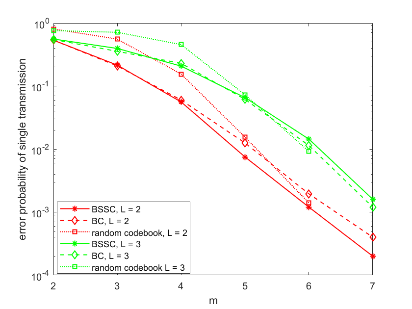
Figure 1: Error probability of Algorithm 2.

Interestingly, BSSCs outperform BCs, despite these codebooks having the same minimum distance. In [13], the same was observed in single-user reconstruction. With increasing $m$, the performance benefit of the algebraically defined codebook over random codebooks diminishes. However, the decoding complexity remains manageable for the algebraic codebooks.

VI Conclusion

We have extended the work [13] by exploiting the geometry of BSSCs. These Grassmannian lines are described as common eigenspaces of maximal sets of commuting Pauli matrices, or equivalently, as columns of Clifford matrices. Further, we have developed a low complexity algorithm for multi BSSCs transmission with low error probability. In future research, we shall consider also noise in multi-user reconstruction, and work toward a practical algorithm along the lines of [11].

References

• [1] P. Viswanath and V. Anantharam, “Optimal sequences and sum capacity of synchronous CDMA systems,” IEEE Trans. Inf. Th., vol. 45, no. 6, pp. 1984–1991, Sep. 1999.
• [2] D. Love, R. Heath, Jr., and T. Strohmer, “Grassmannian beamforming for multiple-input multiple-output wireless systems,” IEEE Trans. Inf. Th., vol. 49, no. 10, pp. 2735–2747, Oct. 2003.
• [3] R. Kötter and F. Kschischang, “Coding for errors and erasures in random network coding,” IEEE Trans. Inf. Th., vol. 54, no. 8, pp. 3579–3591, Aug. 2008.
• [4] R. DeVore, “Deterministic constructions of compressed sensing matrices,” Journal of Complexity, vol. 23, no. 4–6, pp. 918–925, 2007.
• [5] S. D. Howard, A. R. Calderbank, and S. J. Searle, “A fast reconstruction algorithm for deterministic compressive sensing using second order Reed-Muller codes,” in Conference on Information Sciences and Systems, March 2008, pp. 11–15.
• [6] S. Li and G. Ge, “Deterministic sensing matrices arising from near orthogonal systems,” IEEE Trans. Inf. Th., vol. 60, no. 4, pp. 2291–2302, Apr. 2014.
• [7] G. Wang, M.-Y. Niu, and F.-W. Fu, “Deterministic constructions of compressed sensing matrices based on codes,” Cryptography and Communications, Sep. 2018.
• [8] A. Thompson and R. Calderbank, “Compressed neighbour discovery using sparse Kerdock matrices,” in Proc. IEEE ISIT, Jun. 2018, pp. 2286–2290.
• [9] D. Guo and L. Zhang, “Virtual full-duplex wireless communication via rapid on-off-division duplex,” in Allerton Conference on Communication, Control, and Computing, Sep. 2010, pp. 412–419.
• [10] C. Tsai and A. Wu, “Structured random compressed channel sensing for millimeter-wave large-scale antenna systems,” IEEE Trans. Sign. Proc., vol. 66, no. 19, pp. 5096–5110, Oct. 2018.
• [11] R. Calderbank and A. Thompson, “CHIRRUP: a practical algorithm for unsourced multiple access,” Information and Inference: A Journal of the IMA, no. iaz029, 2019, https://doi.org/10.1093/imaiai/iaz029.
• [12] A. Osseiran, J. Monserrat, and P. Marsch, editors, 5G Mobile and Wireless Communications Technology.   Cambridge University Press, 2016.
• [13] O. Tirkkonen and R. Calderbank, “Codebooks of complex lines based on binary subspace chirps,” in IEEE Information Theory Workshop (ITW), 2019, pp. 1–5.
• [14] J. Dehaene and B. D. Moor, “Clifford group, stabilizer states, and linear and quadratic operations over GF(2),” Phys. Rev A, vol. 68, p. 042318, Oct. 2003.
• [15] R. Ranga Rao, “On some explicit formulas in the theory of Weil representation,” vol. 157, no. 2, 1993, pp. 335–371.
• [16] M. A. Nielsen and I. L. Chuang, Quantum computation and quantum information.   Cambridge University Press, Cambridge, 2000.
• [17] N. Rengaswamy, R. Calderbank, S. Kadhe, and H. D. Pfister, “Synthesis of logical Clifford operators via symplectic geometry,” in Proc. IEEE ISIT, Jun. 2018, pp. 791–795, arXiv:1803.06987.
• [18] T. Can, N. Rengaswamy, R. Calderbank, and H. D. Pfister, “Kerdock codes determine unitary 2-designs,” [Online]. Available: https://arxiv.org/abs/1904.07842.
• [19] R. Calderbank, S. Howard, and S. Jafarpour, “Construction of a large class of matrices satisfying a statistical isometry property,” in IEEE Journal of Selected Topics in Signal Processing, Special Issue on Compressive Sensing, vol. 4, no. 2, 2010, pp. 358–374.