Efficient quantization and weak covering of high dimensional cubes

Abstract

Let $\mathbb{Z}_{n}=\{Z_{1},\ldots,Z_{n}\}$ be a design; that is, a collection of $n$ points $Z_{j}\in[-1,1]^{d}$. We study the quality of quantization of $[-1,1]^{d}$ by the points of $\mathbb{Z}_{n}$ and the problem of quality of coverage of $[-1,1]^{d}$ by ${\cal B}_{d}(\mathbb{Z}_{n},r)$, the union of balls centred at $Z_{j}\in\mathbb{Z}_{n}$. We concentrate on the cases where the dimension $d$ is not small ($d\geq 5$) and $n$ is not too large, $n\leq 2^{d}$. We define the design ${\mathbb{D}_{n,\delta}}$ as a $2^{d-1}$ design defined on vertices of the cube $[-\delta,\delta]^{d}$, $0\leq\delta\leq 1$. For this design, we derive a closed-form expression for the quantization error and very accurate approximations for the coverage area vol$([-1,1]^{d}\cap{\cal B}_{d}(\mathbb{Z}_{n},r))$. We provide results of a large-scale numerical investigation confirming the accuracy of the developed approximations and the efficiency of the designs ${\mathbb{D}_{n,\delta}}$.

1 Introduction

1.1 Main notation

• $\|\cdot\|$: the Euclidean norm;

• ${\cal B}_{d}(Z,{r})=\{Y\in\mathbb{R}^{d}:\|Y-Z\|\leq{r}\}$: $d$-dimensional ball of radius $r$ centered at $Z\in\mathbb{R}^{d}$;

• $\mathbb{Z}_{n}=\{Z_{1},\ldots,Z_{n}\}$: a design; that is, a collection of $n$ points $Z_{j}\in\mathbb{R}^{d}$;

• ${\cal B}_{d}(\mathbb{Z}_{n},r)=\bigcup_{j=1}^{n}{\cal B}_{d}(Z_{j},r)$;

• $C_{d}(\mathbb{Z}_{n},r)=$vol$([-1,1]^{d}\cap{\cal B}_{d}(\mathbb{Z}_{n},r))/2^{d}$: the proportion of the cube $[-1,1]^{d}$ covered by ${\cal B}_{d}(\mathbb{Z}_{n},r)$;

• vectors in $\mathbb{R}^{d}$ are row-vectors;

• for any $a\in\mathbb{R}$, $\boldsymbol{a}=(a,a,\ldots,a)\in\mathbb{R}^{d}$.

1.2 Main problems of interest

We will study the following two main characteristics of designs $\mathbb{Z}_{n}=\{Z_{1},\ldots,Z_{n}\}\subset\mathbb{R}^{d}$.

1. Quantization error. Let $X=(x_{1},\ldots,x_{d})$ be uniform random vector on $[-1,1]^{d}$. The mean squared quantization error for a design $\mathbb{Z}_{n}$ is defined by

$$\theta(\mathbb{Z}_{n})=\mathbb{E}_{X}\varrho^{2}(X,\mathbb{Z}_{n})\,,\;\;{\rm where}\;\;\varrho^{2}(X,\mathbb{Z}_{n})=\min_{Z_{i}\in\mathbb{Z}_{n}}\|X-Z_{i}\|^{2}\,.$$ (1)

2. Weak covering. Denote the proportion of the cube $[-1,1]^{d}$ covered by the union of $n$ balls ${\cal B}_{d}(\mathbb{Z}_{n},r)=\bigcup_{j=1}^{n}{\cal B}_{d}(Z_{j},r)$ by

$$\mbox{$C_{d}(\mathbb{Z}_{n},r):=$vol$\left([-1,1]^{d}\cap{\cal B}_{d}(\mathbb{Z}_{n},r)\right)/2^{d}$}\,.$$

For given radius $r>0$, the union of $n$ balls ${\cal B}_{d}(\mathbb{Z}_{n},r)$ makes the $(1-\gamma)$-coverage of the cube $[-1,1]^{d}$ if

$$C_{d}(\mathbb{Z}_{n},r)=1-\gamma\,.$$ (2)

Complete coverage corresponds to $\gamma=0$. In this paper, the complete coverage of $[-1,1]^{d}$ will not be enforced and we will mostly be interested in weak covering, that is, achieving (2) with some small $\gamma>0$.

Two $n$-point designs $\mathbb{Z}_{n}$ and $\mathbb{Z}_{n}^{\prime}$ will be differentiated in terms of performance as follows: (a) $\mathbb{Z}_{n}$ dominates $\mathbb{Z}_{n}^{\prime}$ for quantization if $\theta(\mathbb{Z}_{n})<\theta(\mathbb{Z}_{n}^{\prime})$; (b) if for a given $\gamma\geq 0$, $C_{d}(\mathbb{Z}_{n},r_{1})=C_{d}(\mathbb{Z}_{n}^{\prime},r_{2})=1-\gamma$ and $r_{1}<r_{2}$, then the design $\mathbb{Z}_{n}$ provides a more efficient $(1-\gamma)$-coverage than $\mathbb{Z}_{n}^{\prime}$ and is therefore preferable. In Section 1.4 we extend these definitions by allowing the two designs to have different number of points and, moreover, to have different dimensions.

Numerical construction of $n$-point designs with moderate values of $n$ with good quantization and coverage properties has recently attracted much attention in view of diverse applications in several fields including computer experiments pronzato2012design ; pronzato2017minimax ; santner2003design , global optimization zhigljavsky2021bayesian , function approximation SchabackW2006 ; Wendland2005 and numerical integration pronzato2020bayesian . Such designs are often referred to as space-filling designs. Readers can find many additional references in the citations above. Unlike the exiting literature on space-filling, we concentrate on theoretical properties of a family of very efficient designs and derivation of accurate approximations for the characteristics of interest.

1.3 Relation between quantization and weak coverage

The two characteristics, $C_{d}(\mathbb{Z}_{n},r)$ and $\theta(\mathbb{Z}_{n})$, are related: $C_{d}(\mathbb{Z}_{n},r)$, as a function of $r\geq 0$, is the c.d.f. of the r.v. $\varrho(X,\mathbb{Z}_{n})$ while $\theta(\mathbb{Z}_{n})$ is the second moment of the distribution with this c.d.f.:

$$\theta(\mathbb{Z}_{n})=\int_{r\geq 0}r^{2}dC_{d}(\mathbb{Z}_{n},r)\,.$$ (3)

In particular, this yields that if an $n$-point design $\mathbb{Z}_{n}^{\ast}$ maximizes, in the set of all $n$-point designs, $C_{d}(\mathbb{Z}_{n},r)$ for all $r>0$, then it also minimizes $\theta(\mathbb{Z}_{n})$. Moreover, if r.v. $\varrho(X,\mathbb{Z}_{n})$ stochastically dominates $\varrho(X,\mathbb{Z}_{n}^{\prime})$, so that $C_{d}(\mathbb{Z}_{n}^{\prime},r)\leq C_{d}(\mathbb{Z}_{n},r)$ for all $r\geq 0$ and the inequality is strict for at least one $r$, then $\theta(\mathbb{Z}_{n})<\theta(\mathbb{Z}_{n}^{\prime})$.

The relation (3) can alternatively be written as

$$\theta(\mathbb{Z}_{n})=\int_{r\geq 0}r\,dC_{d}(\mathbb{Z}_{n},\sqrt{r})\,,$$ (4)

where $C_{d}(\mathbb{Z}_{n},\sqrt{r})$, considered as a function of $r$, is the c.d.f. of the r.v. $\varrho^{2}(X,\mathbb{Z}_{n})$ and hence $\theta(\mathbb{Z}_{n})$ is the mean of this r.v. Relation (4) is simply another form of (1).

1.4 Renormalised versions and formulation of optimal design problems

In view of (13), the naturally defined re-normalized version of $\theta(\mathbb{Z}_{n})$ is $Q_{d}(\mathbb{Z}_{n})={n^{2/d}}\theta(\mathbb{Z}_{n})/({4d}).$ From (4) and (3), $Q_{d}(\mathbb{Z}_{n})$ is the expectation of the r.v. ${n^{2/d}}\varrho^{2}(X,\mathbb{Z}_{n})/({4d})$ and the second moment of the r.v. ${n^{1/d}}\varrho(X,\mathbb{Z}_{n})/({2\sqrt{d}})$ respectively. This suggests the following re-normalization of the radius $r$ with respect to $n$ and $d$:

$$R={n^{1/d}}r/({2\sqrt{d}})\,.$$ (5)

We can then define optimal designs as follows. Let $d$ be fixed, ${\cal Z}_{n}=\{\mathbb{Z}_{n}\}$ be the set of all $n$-point designs and ${\cal Z}=\cup_{n=1}^{\infty}{\cal Z}_{n}$ be the set of all designs.

Definition 1

The design $\mathbb{Z}_{m}^{\ast}$ with some $m$ is optimal for quantization in $[-1,1]^{d}$, if

$$Q_{d}(\mathbb{Z}_{m}^{\ast})=\min_{n}\min_{\mathbb{Z}_{n}\in{\cal Z}_{n}}Q_{d}(\mathbb{Z}_{n})=\min_{\mathbb{Z}\in{\cal Z}}Q_{d}(\mathbb{Z})\,.$$ (6)

Definition 2

The design $\mathbb{Z}_{m}^{\ast}$ with some $m$ is optimal for $(1-\gamma)$-coverage of $[-1,1]^{d}$, if

$$R_{1\!-\!\gamma}(\mathbb{Z}_{m}^{\ast})=\min_{n}\min_{\mathbb{Z}_{n}\in{\cal Z}_{n}}R_{1\!-\!\gamma}(\mathbb{Z}_{n})=\min_{\mathbb{Z}\in{\cal Z}}R_{1\!-\!\gamma}(\mathbb{Z})\,.$$ (7)

Here $0\leq\gamma\leq 1$ and for a given design $\mathbb{Z}_{n}\in{\cal Z}_{n}$,

$$R_{1\!-\!\gamma}(\mathbb{Z}_{n})={n^{1/d}}r_{1\!-\!\gamma}(\mathbb{Z}_{n})/({2\sqrt{d}})\,,$$ (8)

where $r_{1\!-\!\gamma}(\mathbb{Z}_{n})$ is defined as the smallest $r$ such that $C_{d}(\mathbb{Z}_{n},r)=1-\gamma$.

Importance of the factor $\sqrt{d}$ in (5) will be seen in Section 3.5 where we shall study the asymptotical behaviour of $(1-\gamma)$-coverings for large $d$.

1.5 Thickness of covering

Let $\gamma=0$ in Definition 2. Then $r_{1}(\mathbb{Z}_{n})$ is the covering radius associated with $\mathbb{Z}_{n}$ so that the union of the balls ${\cal B}_{d}(\mathbb{Z}_{n},r)$ with $r=r_{1}(\mathbb{Z}_{n})$ makes a coverage of $[-1,1]^{d}$. Let us tile up the whole space $\mathbb{R}^{d}$ with the translations of the cube $[-1,1]^{d}$ and corresponding translations of the balls ${\cal B}_{d}(\mathbb{Z}_{n},r)$. This would make a full coverage of the whole space; denote this space coverage by ${\cal B}_{d}(\mathbb{Z}_{(n)},r)$. The thickness $\Theta$ of any space covering is defined, see (Conway, , f-la (1), Ch. 2), as the average number of balls containing a point of the whole space. In our case of ${\cal B}_{d}(\mathbb{Z}_{(n)},r)$, the thickness is

$$\Theta({\cal B}_{d}(\mathbb{Z}_{(n)},r))=\frac{n\,\mbox{vol}\left({\cal B}_{d}(0,r)\right)}{\mbox{vol}([-1,1]^{d})}=\frac{n\,r^{d}\,\mbox{vol}\left({\cal B}_{d}(0,1)\right)}{2^{d}}\,.$$

The normalised thickness, $\theta$, is the thickness $\Theta$ divided by $\mbox{vol}\left({\cal B}_{d}(0,1)\right)$, the volume of the unit ball, see (Conway, , f-la (2), Ch. 2). In the case of ${\cal B}_{d}(\mathbb{Z}_{(n)},r)$, the normalised thickness is

$$\theta({\cal B}_{d}(\mathbb{Z}_{(n)},r))=\frac{n\,r^{d}}{2^{d}}=d^{d/2}\,\left[R_{1}(\mathbb{Z}_{(n)})\right]^{d}\,\,,$$

where we have recalled that $r=r_{1}(\mathbb{Z}_{n})$ and $R_{1\!-\!\gamma}(\mathbb{Z}_{n})={n^{1/d}}r_{1\!-\!\gamma}(\mathbb{Z}_{n})/({2\sqrt{d}})$ for any $0\leq\gamma\leq 1$.

We can thus define the normalised thickness of the covering of the cube by the same formula and extend it to any $0\leq\gamma\leq 1$:

Definition 3

Let ${\cal B}_{d}(\mathbb{Z}_{n},r)$ be a $(1-\gamma)$-coverage of the cube $[-1,1]^{d}$ with $0\leq\gamma\leq 1$. Its normalised thickness is defined by

$$\theta({\cal B}_{d}(\mathbb{Z}_{n},r))=(\sqrt{d}R)^{d}\,,$$ (9)

where $R=n^{1/d}r/({2\sqrt{d}})$, see (5).

In view of (9), we can reformulate the definition (7) of the $(1-\gamma)$-covering optimal design by saying that this design minimizes (normalised) thickness in the set of all $(1-\gamma)$-covering designs.

1.6 The design of the main interest

We will be mostly interested in the following $n$-point design $\mathbb{Z}_{n}={\mathbb{D}_{n,\delta}}$ defined only for $n=2^{d-1}$:

Design ${\mathbb{D}_{n,\delta}}$: a $2^{d-1}$ design defined on vertices of the cube $[-\delta,\delta]^{d}$, $0\leq\delta\leq 1$.

For theoretical comparison with design ${\mathbb{D}_{n,\delta}}$, we shall consider the following simple design, which extends to the integer point lattice $Z^{d}$ (shifted by ${\boldsymbol{\frac{1}{2}}}$) in the whole space $\mathbb{R}^{d}$:

Design ${\mathbb{D}_{n}^{(0)}}$: the collection of $2^{d}$ points $(\pm\frac{1}{2},\ldots,\pm\frac{1}{2})$, all vertices of the cube $[-\frac{1}{2},\frac{1}{2}]^{d}$.

Without loss of generality, while considering the design ${\mathbb{D}_{n,\delta}}$ we assume that the point $Z_{1}\in{\mathbb{D}_{n,\delta}}=\{Z_{1},\ldots,Z_{n}\}$ is $Z_{1}={\boldsymbol{\delta}}=(\delta,\ldots,\delta)$. Similarly, the first point in ${\mathbb{D}_{n}^{(0)}}$ is $Z_{1}={\boldsymbol{\frac{1}{2}}}=(\frac{1}{2},\ldots,\frac{1}{2})$. Note also that for numerical comparisons, in Section 4 we shall introduce one more design.

The design ${\mathbb{D}_{n,{1/2}}}$ extends to the lattice $D_{d}$ (shifted by ${\boldsymbol{\frac{1}{2}}}$) containing points $X=(x_{1},\ldots,x_{d})$ with integer components satisfying $x_{1}+\ldots+x_{d}=0\;(\!\!\!\!\mod 2)$, see (Conway, , Sect. 7.1, Ch. 4); this lattice is sometimes called ‘checkerboard lattice’. The motivation to theoretically study the design ${\mathbb{D}}_{n,\delta}$ is a consequence of numerical results reported in us and second_paper , where the present authors have considered $n$-point designs in $d$-dimensional cubes providing good coverage and quantization and have shown that for all dimensions $d\geq 7$, the design ${\mathbb{D}}_{n,\delta}$ with suitable $\delta$ provides the best quantization and coverage per point among all other designs considered. Aiming at practical applications mentioned in Section 1.2, our aim was to consider the designs with $n$ which is not too large and in any case does not exceed $2^{d}$.

If the number of points $n$ in a design is much larger than $2^{d}$, then we may use the following scheme of construction of efficient quantizers in the cube $[-1,1]^{d}$: (a) construct one of the very efficient lattice space quantizers, see (Conway, , Sect. 3, Ch. 2), (b) take the lattice points belonging to a very large cube, and (c) scale the chosen large cube to $[-1,1]^{d}$. In view of Theorem 8.9 in graf2007foundations , as $n\to\infty$, the normalised quantization error $Q_{d}(\mathbb{Z}_{n})$ of the sequence of resulting designs $\mathbb{Z}_{n}$ converges to the respective quantization error of the lattice space quantizer. However, for any given $n$ the study of quantization error of such designs is difficult (both, numerically and theoretically) as there could be several non-congruent types of Voronoi cells due to boundary conditions. Note also that the boundary conditions make significant difference in relative efficiencies of the resulting designs. In particular, the checkerboard lattice $D_{d}$ is better than the integer-point lattice $\mathbb{Z}^{d}$ for all $d\geq 3$ as a space quantizer and becomes the best lattice space quantizer for $d=4$ but in the case of cube $[-1,1]^{d}$, the design ${\mathbb{D}_{n,\delta}}$ (with optimal $\delta$) makes a better quantizer than ${\mathbb{D}_{n}^{(0)}}$ for $d\geq 7$ only; see Section 2.4 for theoretical and numerical comparison of the two designs.

1.7 Structure of the rest of the paper and the main results

In Section 2 we study $Q_{d}(\mathbb{D}_{n,\delta})$, the normalized mean squared quantization error for the design ${\mathbb{D}_{n,\delta}}$. There are two important results, Theorems 2.1 and 2.2. In Theorem 2.1, we derive the explicit form for the Voronoi cells for the points of the design ${\mathbb{D}_{n,\delta}}$ and in Theorem 2.2 we derive a closed-form expression for $Q_{d}(\mathbb{D}_{n,\delta})$ for any $\delta>0$. As a consequence, in Corollary 1 we determine the optimal value of $\delta$.

The main result of Section 3 is Theorem 3.1, where we derive closed-form expressions (in terms of $C_{d,Z,{r}}$, the fraction of the cube $[-1,1]^{d}$ covered by a ball ${\cal B}_{d}(Z,{r})$) for the coverage area with vol$\left([-1,1]^{d}\cap{\cal B}_{d}(\mathbb{Z}_{n},r)\right)$. Then, using accurate approximations for $C_{d,Z,{r}}$, we derive approximations for vol$\left([-1,1]^{d}\cap{\cal B}_{d}(\mathbb{Z}_{n},r)\right)$. In Theorem 3.2 we derive asymptotic expressions for the $(1-\gamma)$-coverage radius for the design ${\mathbb{D}_{d,1/2}}$ and show that for any $\gamma>0$, the ratio of the $(1-\gamma)$-coverage radius to the $1$-coverage radius tends to $1/\sqrt{3}$ as $d\to\infty$. Numerical results of Section 3.5 confirm that even for rather small $d$, the $0.999$-coverage radius is much smaller than the $1$-coverage radius providing the full coverage.

In Section 4 we demonstrate that the approximations developed in Section 3 are very accurate and make a comparative study of selected designs used for quantization and covering.

In Appendices A–C, we provide proofs of the most technical results. In Appendix D, for completeness, we briefly derive an approximation for $C_{d,Z,{r}}$ with arbitrary $d$, $Z$ and $r$.

The two most important contributions of this paper are: a) derivation of the closed-form expression for the quantization error for the design ${\mathbb{D}_{n,\delta}}$, and b) derivation of accurate approximations for the coverage area vol$\left([-1,1]^{d}\cap{\cal B}_{d}(\mathbb{Z}_{n},r)\right)$ for the design ${\mathbb{D}_{n,\delta}}$.

2 Quantization

2.1 Reformulation in terms of the Voronoi cells

Consider any $n$-point design $\mathbb{Z}_{n}=\{Z_{1},\ldots,Z_{n}\}$. The Voronoi cell $V(Z_{i})$ for $Z_{i}\in\mathbb{Z}_{n}$ is defined as

$$V(Z_{i})=\{x\in[-1,1]^{d}:\left\lVert Z_{i}-x\right\rVert\leq\left\lVert Z_{j}-x\right\rVert\text{ for }j\neq i\}\,.$$

The mean squared quantization error $\theta(\mathbb{Z}_{n})$ introduced in (1) can be written in terms of the Voronoi cells as follows:

$$\theta(\mathbb{Z}_{n})=\mathbb{E}_{X}\min_{i=1,\ldots,n}\|X-Z_{i}\|^{2}=\frac{1}{{\rm vol([-1,1]^{d})}}\sum_{i=1}^{n}\int_{V(Z_{i})}\left\lVert X-Z_{i}\right\rVert^{2}dX\,,$$ (10)

where $X=(x_{1},\ldots,x_{d})$ and $dX=dx_{1}dx_{2}\cdots dx_{d}$.

This reformulation has significant benefit when the design $\mathbb{Z}_{n}$ has certain structure. In particular, if all of the Voronoi cells $V(Z_{i}),i=1,\ldots,n,$ are congruent, then we can simplify (10) to

$$\theta(\mathbb{Z}_{n})=\frac{1}{{\rm vol}(V(Z_{1}))}\int_{V(Z_{1})}\left\lVert X-Z_{1}\right\rVert^{2}dX\,.$$ (11)

In Section 2.4, this formula will be the starting point for derivation of the closed-form expression for $\theta(\mathbb{Z}_{n})$ for the design $\mathbb{D}_{n,\delta}$.

2.2 Re-normalization of the quantization error

To compare efficiency of $n$-point designs $\mathbb{Z}_{n}$ with different values of $n$, one must suitably normalise $\theta(\mathbb{Z}_{n})$ with respect to $n$. Specialising a classical characteristic for quantization in space, as formulated in (Conway, , f-la (86), Ch.2), we obtain

$$Q_{d}(\mathbb{Z}_{n})=\frac{1}{d}\frac{\frac{1}{n}\sum_{i=1}^{n}\int_{V(Z_{i})}\left\lVert X-Z_{i}\right\rVert^{2}dX}{\left[\frac{1}{n}\sum_{i=1}^{n}{\rm vol}(V(Z_{i}))\right]^{1+\frac{2}{d}}}\,.$$ (12)

Note that $Q_{d}(\mathbb{Z}_{n})$ is re-normalised with respect to dimension $d$ too, not only with respect to $n$. Normalization $1/d$ with respect to $d$ is very natual in view of the definition of the Euclidean norm.

Using (10), for the cube $[-1,1]^{d}$, (12) can be expressed as

$$Q_{d}(\mathbb{Z}_{n})=\frac{n^{2/d}\theta(\mathbb{Z}_{n})}{d\left[\sum_{i=1}^{n}{\rm vol}(V(Z_{i}))\right]^{2/d}}=\frac{n^{2/d}\theta(\mathbb{Z}_{n})}{d\cdot{\rm vol}([-1,1]^{d})^{2/d}}=\frac{n^{2/d}}{4d}\theta(\mathbb{Z}_{n})\,.$$ (13)

2.3 Voronoi cells for $\mathbb{D}_{n,\delta}$

Proposition 1

Consider the design ${\mathbb{D}_{n,\delta}^{(0)}}$, the collection of $n=2^{d}$ points $(\pm\delta,\ldots,\pm\delta)$, $0<\delta<1$. The Voronoi cells for this design are all congruent. The Voronoi cell for the point $\boldsymbol{\delta}=(\delta,\delta,\ldots,\delta)$ is the cube

$$C_{0}=\left\{X\!=\!(x_{1},\ldots,x_{d})\!\in\!\mathbb{R}^{d}\!:\;0\leq x_{i}\leq 1,\;i=1,2,\ldots,d\right\}\,.$$ (14)

$\mathbf{Proof}$. Consider the Voronoi cells created by the design ${\mathbb{D}_{n,\delta}^{(0)}}$ in the whole space $\mathbb{R}^{d}$. For the point $\boldsymbol{\delta}=(\delta,\delta,\ldots,\delta)$, the Voronoi cell is clearly $\{X\!=\!(x_{1},\ldots,x_{d})\!:\,x_{i}\geq 0\}$. By intersecting this set with the cube $[-1,1]^{d}$ we obtain (14). $\Box$

Theorem 2.1

The Voronoi cells of the design $\mathbb{D}_{n,\delta}=\{Z_{1},\ldots,Z_{n}\}$ are all congruent. The Voronoi cell for the point $Z_{1}=\boldsymbol{\delta}=(\delta,\delta,\ldots,\delta)\in\mathbb{R}^{d}$ is

$$V(Z_{1})=C_{0}\bigcup\left[\bigcup_{j=1}^{d}U_{j}\right]$$ (15)

where $C_{0}$ is the cube (14) and

$$U_{j}=\left\{X=(x_{1},x_{2},\ldots,x_{d})\!\in\!\mathbb{R}^{d}\!:-1\leq x_{j}\leq 0,|x_{j}|\leq x_{k}\leq 1\;\mbox{ \rm for all }k\neq j\right\}\,.$$ (16)

The volume of $V(Z_{1})$ is ${{\rm vol}(V(Z_{1}))}=2$.

$\mathbf{Proof}$. The design $\mathbb{D}_{n,\delta}$ is symmetric with respect to all components implying that all $n=2^{d-1}$ Voronoi cells are congruent immediately yielding that their volumes equal 2. Consider $V(Z_{1})$ with $Z_{1}=\boldsymbol{\delta}$.

Since $\mathbb{D}_{n,\delta}\subset{\mathbb{D}_{n,\delta}^{(0)}}$, where design ${\mathbb{D}_{n,\delta}^{(0)}}$ is introduced in Proposition 1, and $C_{0}$ is the Voronoi set of $\boldsymbol{\delta}$ for design ${\mathbb{D}_{n,\delta}^{(0)}}$, $C_{0}\subset V(\boldsymbol{\delta})$ for design $\mathbb{D}_{n,\delta}$ too.

Consider the $d$ cubes adjacent to $C_{0}$:

$$C_{j}=\left\{X=(x_{1},x_{2},\ldots,x_{d})\!\in\!\mathbb{R}^{d}\!:-1\leq x_{j}\leq 0,\;0\leq x_{i}\leq 1\;\mbox{ \rm for all }i\neq j\right\}\,;\;\;j=1,\ldots,d.$$ (17)

A part of each cube $C_{j}$ belongs to $V(Z_{1})$. This part is exactly the set $U_{j}$ defined by (16). This can be seen as follows. A part of $C_{j}$ also belongs to the Voronoi set of the point $X_{jk}=\boldsymbol{\delta}-2\delta e_{j}-2\delta e_{k}$, where $e_{l}=(0,\ldots,0,1,0,\ldots,0)$ with 1 placed at $l$-th place; all components of $X_{jk}$ are $\delta$ except $j$-th and $k$-th components which are $-\delta$. We have to have $|x_{j}|\leq x_{k}$, for a point $X\in C_{j}$ to be closer to $Z_{1}$ than to $X_{jk}$. Joining all constraints for $X=(x_{1},x_{2},\ldots,x_{d})\in C_{j}$ ($k=1,\ldots,d$, $k\neq j$) we obtain (16) and hence (15).

$\Box$

2.4 Explicit formulae for the quantization error

Theorem 2.2

For the design $\mathbb{D}_{n,\delta}$ with $0\leq\delta\leq 1$, we obtain:

$$\theta(\mathbb{D}_{n,\delta}) = d\left(\delta^{2}-\delta+\frac{1}{3}\right)+\frac{2\delta}{d+1}\,,$$ (18)

$$Q_{d}(\mathbb{D}_{n,\delta}) = 2^{-2/d}\left(\delta^{2}-\delta+\frac{1}{3}+\frac{2\delta}{d(d+1)}\right)\,.$$ (19)

$\mathbf{Proof}$. To compute $\theta(\mathbb{D}_{n,\delta})$, we use (11), where, in view of Theorem 2.1, ${{\rm vol}(V(Z_{1}))}=2$. Using the expression (15) for $V(Z_{1})$ with $Z_{1}=\boldsymbol{\delta}$, we obtain

$$\theta(\mathbb{Z}_{n})=\frac{1}{2}\int_{V(Z_{1})}\left\lVert X-Z_{1}\right\rVert^{2}dX=\frac{1}{2}\left[\int_{C_{0}}\left\lVert X-Z_{1}\right\rVert^{2}dX+d\int_{U_{1}}\left\lVert X-Z_{1}\right\rVert^{2}dX\right]\,.$$ (20)

Consider the two terms in (20) separately. The first term is easy:

$$\int_{C_{0}}\left\lVert X-Z_{1}\right\rVert^{2}dX=\int_{C_{0}}\sum_{i=1}^{d}(x_{i}-\delta)^{2}dx_{1}\ldots dx_{d}=d\int_{0}^{1}(x-\delta)^{2}dx=d\left(\delta^{2}-\delta+\frac{1}{3}\right)\,.$$ (21)

For the second term we have:

$$\!\!\!\!\!\!\int_{U_{1}}\left\lVert X-Z_{1}\right\rVert^{2}dX = \int_{-1}^{0}\left[\int_{|x_{1}|}^{1}\ldots\int_{|x_{1}|}^{1}\sum_{i=1}^{d}(x_{i}-\delta)^{2}dx_{2}\ldots dx_{d}\right]dx_{1}$$ (22)

$$= \int_{-1}^{0}(x_{1}-\delta)^{2}(1+x_{1})^{d-1}dx_{1}+(d-1)\int_{-1}^{0}(1+x_{1})^{d-2}\int_{|x_{1}|}^{1}(x_{2}-\delta)^{2}dx_{2}dx_{1}$$

$$= \delta^{2}-\delta+\frac{1}{3}+\frac{4\delta}{d(d+1)}\,.$$

Inserting the obtained expressions into (20) we obtain (18). The expression (19) is a consequence of (13), (18) and $n=2^{d-1}$. $\Box$

A simple consequence of Theorem 2.2 is the following corollary.

Corollary 1

The optimal value of $\delta$ minimising $\theta(\mathbb{D}_{n,\delta})$ and $Q_{d}(\mathbb{D}_{n,\delta})$ is

$$\delta^{\ast}=\frac{1}{2}-\frac{1}{d(d+1)}\,;$$ (23)

for this value,

$$Q_{d}(\mathbb{D}_{n,\delta^{\ast}})=\min_{\delta}Q_{d}(\mathbb{D}_{n,\delta})=2^{-2/d}\left[\frac{1}{12}+{\frac{{d}^{2}+d-1}{\left(d+1\right)^{2}{d}^{2}}}\right]\,.$$ (24)

Let us make several remarks.

1. The value $\delta^{\ast}$ can be alternatively characterised by the well-known optimality condition of a general design saying that each design point of an optimal quantizer must be a centroid of the related Voronoi cell; see e.g. saka2007latinized . Specifically, each design points $Z_{i}\in{\mathbb{D}_{n,\delta}}$ is the centroid of $V(Z_{i})$ if and only if $\delta=\delta^{\ast}$.

2. From (19), for the design $\mathbb{D}_{n,1/2}$ we get

   $$Q_{d}(\mathbb{D}_{n,1/2})=2^{-2/d}\left[\frac{1}{12}+\frac{1}{\left(d+1\right)d}\right]\,;$$ (25)

   this value is always slightly larger than (24).

3. For the one-point design $\mathbb{D}^{(0)}=\{0\}$ with the single point 0 and the design $\mathbb{D}_{n}^{(0)}$ with $n=2^{d}$ points $(\pm\frac{1}{2},\ldots,\pm\frac{1}{2})$ we have $Q_{d}(\mathbb{D}^{(0)})=Q_{d}(\mathbb{D}_{n}^{(0)})=1/12$, which coincides with the value of $Q_{d}$ in the case of space quantization by the integer-point lattice $Z^{d}$, see (Conway, , Ch. 2 and 21).

4. The quantization error (25) for the design ${\mathbb{D}_{n,1/2}}$ have almost exactly the same form as the quantization error for the ‘checkerboard lattice’ $D_{d}$ in $\mathbb{R}^{d}$; the difference is in the factor $1/2$ in the last term in (25), see (Conway, , f-la (27), Ch.21). Naturally, the quantization error $Q_{d}$ for $D_{d}$ in $\mathbb{R}^{d}$ is slightly smaller than $Q_{d}$ for $\mathbb{D}_{n,1/2}$ in $[-1,1]^{d}$.

5. The optimal value of $\delta$ in (23) is smaller than $1/2$. This is caused by a non-symmetrical shape of the Voronoi cells $V(Z_{j})$ for designs $\mathbb{D}_{n,\delta}$, which is clearly visible in (15).

6. The minimal value of $Q_{d}(\mathbb{D}_{n,\delta^{\ast}})$ with respect to $d$ is attained at $d=15$.

7. Formulas (23) and (24) are in agreement with numerical results presented in Table 4 of us and Table 5 of second_paper .

Let us now briefly illustrate the results above. In Figure 2, the black circles depict the quantity $Q_{d}(\mathbb{D}_{n,\delta^{\ast}})$ as a function of $d$. The quantity $Q_{d}(\mathbb{D}_{n}^{(0)})=1/12$ is shown with the solid red line. We conclude that from dimension seven onwards, the design $\mathbb{D}_{n,\delta^{\ast}}$ provides better quantization per points than the design $\mathbb{D}_{n}^{(0)}$. Moreover for $d>15$, the quantity $Q_{d}(\mathbb{D}_{n,\delta^{\ast}})$ slowly increases and converges to $1/12$. Typical behaviour of $Q_{d}(\mathbb{D}_{n,\delta})$ as a function of $\delta$ is shown in Figure 2. This figure demonstrates the significance of choosing $\delta$ optimally.

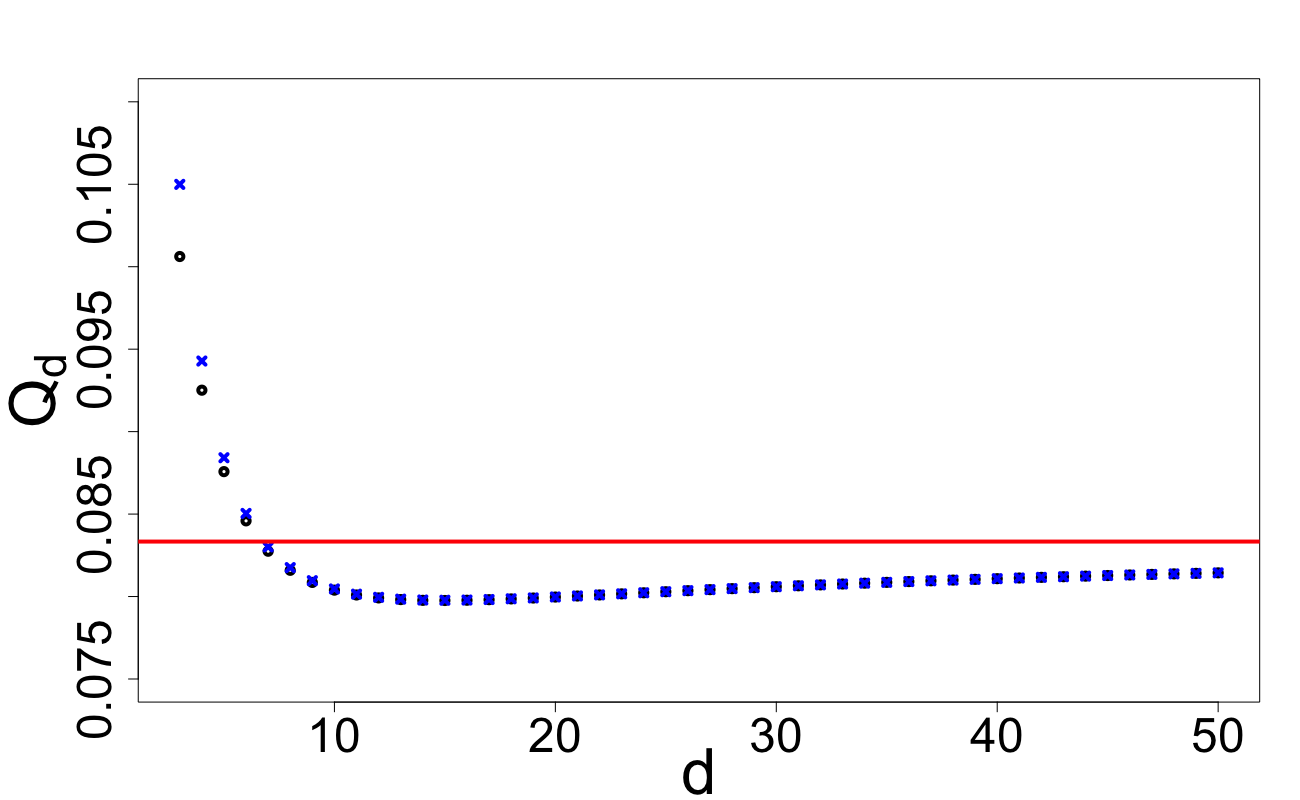
Figure 1: $Q_{d}(\mathbb{D}_{n,\delta^{\ast}})$ and $Q_{d}(\mathbb{D}_{n,1/2})$ as functions
of $d$ and $Q_{d}(\mathbb{D}_{n}^{(0)})=1/12$; $d=3,\ldots,50$.

Figure 2: $Q_{d}(\mathbb{D}_{n,\delta})$ as a function of $\delta$ and
$Q_{d}(\mathbb{D}_{n}^{(0)})=1/12$; $d=10$.

3 Closed-form expressions for the coverage area with $\mathbb{D}_{n,\delta}$ and approximations

In this section, we will derive explicit expressions for the coverage area of the cube $[-1,1]^{d}$ by the union of the balls ${\cal B}_{d}({\mathbb{D}_{n,\delta}},r)$ associated with the design ${\mathbb{D}_{n,\delta}}$ introduced in Section 1.2. That is, we will derive expressions for the quantity $C_{d}(\mathbb{D}_{n,\delta},r)$ for all values of $r$. Then, in Section 3.3, we shall obtain approximations for $C_{d}(\mathbb{D}_{n,\delta},r)$. The accuracy of the approximations will be assessed in Section 4.2.

3.1 Reduction to Voronoi cells

For an $n$-point design $\mathbb{Z}_{n}=\{Z_{1},\ldots,Z_{n}\}$, denote the proportion of the Voronoi cell around $Z_{i}$ covered by the ball ${\cal B}_{d}(Z_{i},{r})$ as

$$V_{d,Z_{i},{r}}:={\rm vol}(V(Z_{i})\cap{\cal B}_{d}(Z_{i},{r}))/{\rm vol}(V(Z_{i}))\,.$$

The following lemma is straightforward.

Lemma 1

Consider a design $\mathbb{Z}_{n}=\{Z_{1},\ldots,Z_{n}\}$ such that all Voronoi cells $V(Z_{i})$ are congruent. Then for any $Z_{i}\in\mathbb{Z}_{n}$, $C_{d}(\mathbb{Z}_{n},r)=V_{d,Z_{i},{r}}$.

In view of Theorem 2.1, for design $\mathbb{D}_{n,\delta}$ all Voronoi cells $V(Z_{i})$ are congruent and ${\rm vol}(V(Z_{i}))=2$; recall that $n=2^{d-1}$. By then applying Lemma 1 and without loss of generality we have choosen $Z_{1}=\boldsymbol{\delta}=(\delta,\delta,\ldots,\delta)\in\mathbb{R}^{d}$, we have for any $r>0$

$$V_{d,\boldsymbol{\delta},{r}}=\frac{1}{2}{\rm vol}(V(\boldsymbol{\delta})\cap{\cal B}_{d}(\boldsymbol{\delta},{r}))=C_{d}(\mathbb{D}_{n,\delta},r)\,.$$ (26)

In order to formulate explicit expressions for $V_{d,\boldsymbol{\delta},{r}}$, we need the important quantity, proportion of intersection of $[-1,1]^{d}$ with one ball. Take the cube $[-1,1]^{d}$ and a ball ${\cal B}_{d}(Z,{r})=\{Y\in\mathbb{R}^{d}:\|Y-Z\|\leq{r}\}$ centered at a point $Z=(z_{1},\ldots,z_{d})\in\mathbb{R}^{d}$; this point $Z$ could be outside $[-1,1]^{d}$. The fraction of the cube $[-1,1]^{d}$ covered by the ball ${\cal B}_{d}(Z,{r})$ is denoted by

$$C_{d,Z,{r}}={{\rm vol}([-1,1]^{d}\cap{\cal B}_{d}(Z,{r}))}/2^{d}\,.$$

3.2 Expressing $C_{d}(\mathbb{D}_{n,\delta},r)$ through $C_{d,Z,{r}}$

Theorem 3.1

Depending on the values of $r$ and $\delta$, the quantity $C_{d}(\mathbb{D}_{n,\delta},r)$ can be expressed through $C_{d,Z,{r}}$ for suitable $Z$ as follows.

• For $r\leq\delta$:

  $$C_{d}(\mathbb{D}_{n,\delta},r)=\frac{1}{2}C_{d,\boldsymbol{2\delta-1},{2r}}\,.$$ (27)

• For $\delta\leq r\leq 1+\delta$:

  $$C_{d}(\mathbb{D}_{n,\delta},r) = \frac{1}{2}\left[C_{d,\boldsymbol{2\delta-1},{2r}}+d\int_{0}^{r-\delta}C_{d-1,\boldsymbol{\frac{2\delta-1-{t}}{1-{t}}},{\frac{2\sqrt{r^{2}-(t+\delta)^{2}}}{1-t}}}(1-t)^{d-1}\,dt\right]\,.$$ (28)

• For $r\geq 1+\delta$:

  $$C_{d}(\mathbb{D}_{n,\delta},r)=\frac{1}{2}\left[C_{d,\boldsymbol{2\delta-1},{2r}}+d\int_{0}^{1}C_{d-1,\boldsymbol{\frac{2\delta-1-{t}}{1-{t}}},{\frac{2\sqrt{r^{2}-(t+\delta)^{2}}}{1-t}}}(1-t)^{d-1}\,dt\right]\,.$$ (29)

The proof of Theorem 3.1 is given in Appendix A.

3.3 Approximation for $C_{d}(\mathbb{D}_{n,\delta},r)$

Accurate approximations for $C_{d,Z,{r}}$ for arbitrary $d,Z$ and $r$ were developed in us . By using the general expansion in the central limit theorem for sums of independent non-identical r.v., the following approximation was developed:

$$C_{d,Z,{r}}\cong\Phi(t)+\frac{\|Z\|^{2}+d/63}{5\sqrt{3}(\|Z\|^{2}+d/15)^{3/2}}(1-t^{2})\varphi(t)\,,$$ (30)

where

$$t=\frac{\sqrt{3}(r^{2}-\|Z\|^{2}-d/3)}{2\sqrt{\|Z\|^{2}+{d}/{15}}}\,.$$

A short derivation of this approximation is included in Appendix D. Using (30), we formulate the following approximation for $C_{d}(\mathbb{D}_{n,\delta},r)$.

Approximations for $C_{d}(\mathbb{D}_{n,\delta},r)$. Approximate the values $C_{\cdot,\cdot,\cdot}$ in formulas (27),(28),(29) with corresponding approximations (30).

3.4 Simple bounds for $C_{d}(\mathbb{D}_{n,\delta},r)$

Lemma 2

For any $r\geq 0$, $0<\delta<1$ and $\boldsymbol{\delta}=(\delta,\delta,\ldots,\delta)\in\mathbb{R}^{d}$, the quantity $C_{d}(\mathbb{D}_{n,\delta},r)$ can be bounded as follows:

$$\frac{1}{2}[C_{d,\boldsymbol{2\delta-1},{2r}}+C_{d,A,{2r}}]\leq C_{d}(\mathbb{D}_{n,\delta},r)\leq C_{d,\boldsymbol{2\delta-1},{2r}}\,.$$ (31)

where $A=\left(2\delta+1,2\delta-1,\ldots,2\delta-1\right)\in\mathbb{R}^{d}$.

The proof of Lemma 2 is given in Appendix B.

In Figures 4 and 4, using the approximation given in (30) we study the tightness of the bounds given in (31). In these figures, the dashed red line, dashed blue line and solid black line depict the upper bound, the lower bound and the approximation for $C_{d}(\mathbb{D}_{n,\delta},r)$ respectively. We see that the upper bound is very sharp across $r$ and $d$; this behaviour is not seen with the lower bound.

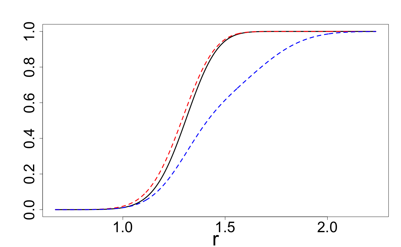
Figure 3: $C_{d}(\mathbb{D}_{n,\delta},r)$ with upper and lower bounds:
$d=20$.

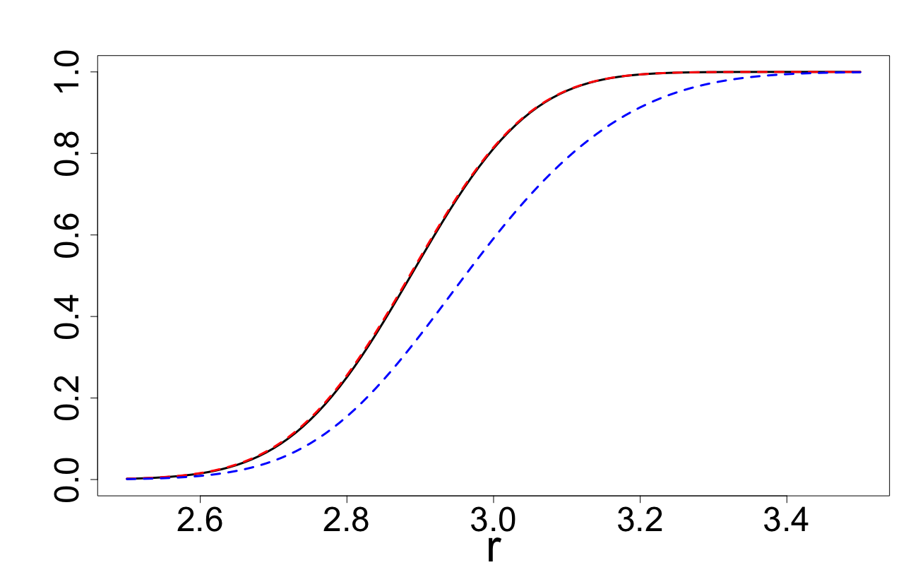
Figure 4: $C_{d}(\mathbb{D}_{n,\delta},r)$ with upper and lower bounds:
$d=100$.

3.5 ‘Do not try to cover the vertices’

In this section, we theoretically support the recommendation ‘do not try to cover the vertices’ which was first stated in us and supported in second_paper on the basis of numerical evidence. In other words, we will show on the example of the design $\mathbb{D}_{n,1/2}$ that in large dimensions the attempt to cover the whole cube rather than 0.999 of it leads to a dramatic increase of the required radius of the balls.

Theorem 3.2

Let $\gamma$ be fixed, $0\leq\gamma\leq 1$. Consider $(1-\gamma)$-coverings of $[-1,1]^{d}$ generated by the designs ${\mathbb{D}_{n,\delta}}$ and the associated normalized radii $R_{1\!-\!\gamma}({\mathbb{D}_{n,\delta}})$, see (8). For any $0<\gamma<1$ and $0\leq\delta\leq 1$, the limit of $R_{1\!-\!\gamma}({\mathbb{D}_{n,\delta}})$, as $d\rightarrow\infty$, exists and achieves minimal value for $\delta=1/2$. Moreover, $R_{1\!-\!\gamma}({\mathbb{D}_{n,1/2}})/R_{1}({\mathbb{D}_{n,1/2}})\rightarrow 1/\sqrt{3}$ as $d\rightarrow\infty,$ for any $0<\gamma<1$.

Proof is given in Appendix C.

In Figures 6-6 using a solid red line we depict the approximation of $C_{d}({\mathbb{D}_{n,1/2}},r)$ as a function of $R={n^{1/d}}r/({2\sqrt{d}})$, see (5). The vertical green line illustrates the value of $R_{0.999}$ and the vertical blue line depicts $R_{1}={n^{1/d}}\sqrt{d+8}/({4\sqrt{d}})$. These figures illustrate that as $d$ increases, for all $\gamma$ we have $R_{1-\gamma}/R_{1}$ slowly tending to $1/\sqrt{3}$. From the proof of Theorem 3.2, it transpires that $C_{d}({\mathbb{D}_{n,\delta}},r)$ as a function of $R$ converges to the jump function with the jump at $1/(2\sqrt{3})$.

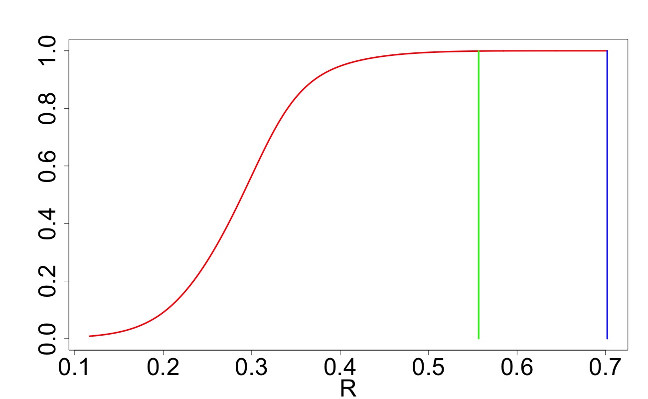
Figure 5: $C_{d}({\mathbb{D}_{n,1/2}},r)$ with $R_{0.999}$ and $R_{1}$: $d=5$.

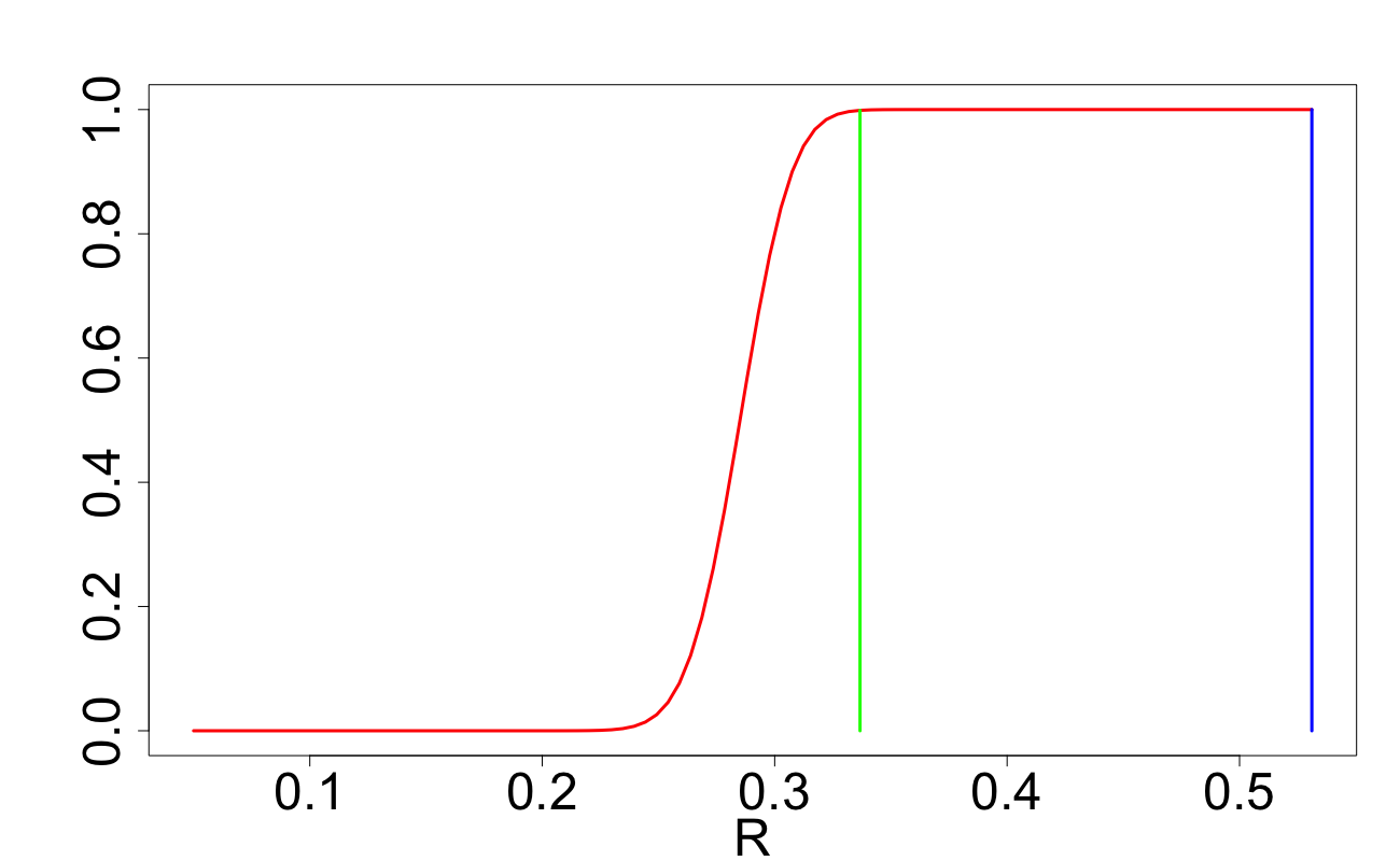
Figure 6: $C_{d}({\mathbb{D}_{n,1/2}},r)$ with $R_{0.999}$ and $R_{1}$: $d=50$.

4 Numerical studies

For comparative purposes, we introduce another design which is one of the most popular designs (both, for quantization and covering) considered in applications.

Design $\mathbb{S}_{n}$: $Z_{1},\ldots,Z_{n}$ are taken from a low-discrepancy Sobol’s sequence on the cube $[-1,1]^{d}$.

For constructing the design $\mathbb{S}_{n}$, we use the R-implementation provided in the well-known ‘SobolSequence’ package Sobol . For $\mathbb{S}_{n}$, we have set $n=1024$ and $F2=10$ (an input parameter for the Sobol sequence function). Sobol sequences $\mathbb{S}_{n}$ attain their best space-filling properties when $n$ is a power of $2$; that is, when $n=2^{\ell}$ for some integer $\ell$. We have chosen $\ell=10$. As we study renormalised characteristics $Q_{d}(\cdot)$ and $R_{1\!-\!\gamma}(\cdot)$ of designs, exact value of $\ell$ for $\mathbb{S}_{n}$ with $n=2^{\ell}$ is almost irrelevant: in particular, numerically computed values $Q_{d}(\mathbb{S}_{2^{\ell}})$ and $R_{1\!-\!\gamma}(\mathbb{S}_{2^{\ell}})$ for $\ell=8,9,11,12$ are almost indistinguishable from the corresponding values for $\ell=10$ provided below in Tables 1 and  2. By varying values of $\ell$, we are not improving space-filling properties of $\mathbb{S}_{2^{\ell}}$. In fact, increase of $\ell$ generally leads to a slight deterioration of normalised space-filling characteristics (including $Q_{d}(\cdot)$ and $R_{1\!-\!\gamma}(\cdot)$) of Sobol sequences.

4.1 Quantization and weak covering comparisons

In Table 1, we compare the normalised mean squared quantization error $Q_{d}(\mathbb{Z}_{n})$ defined in (13) across three designs: $\mathbb{D}_{n,\delta^{\ast}}$ with $\delta^{\ast}$ given in (23), $\mathbb{D}_{n}^{(0)}$ and $\mathbb{S}_{n}$.

	$d=5$	$d=7$	$d=10$	$d=15$	$d=20$
$Q_{d}(\mathbb{D}_{n,\delta^{\ast}})$	0.0876	0.0827	0.0804	0.0798	0.0800
$Q_{d}(\mathbb{D}_{n}^{(0)})$	0.0833	0.0833	0.0833	0.0833	0.0833
$Q_{d}(\mathbb{S}_{n})$	0.0988	0.1003	0.1022	0.1060	0.1086

Table 1: Normalised mean squared quantization error $Q_{d}$ for three designs and different $d$.

In Table 2, we compare the normalised statistic $R_{1\!-\!\gamma}$ introduced in (7), where we have fixed $\gamma=0.01$. For designs $\mathbb{D}_{n,\delta}$ (with the optimal value of $\delta$), $\mathbb{D}_{n,{\tiny 1/2}}$ and $\mathbb{D}_{n}^{(0)}$ we have also included $R_{1}$, the smallest normalised radius that ensures the full coverage.

	$d=5$	$d=7$	$d=10$	$d=15$	$d=20$
$R_{1\!-\!\gamma}(\mathbb{D}_{n,\delta})$	0.4750 (0.54)	0.3992 (0.53)	0.3635 (0.52)	0.3483 (0.51)	0.3417 (0.50)
$R_{1\!-\!\gamma}(\mathbb{D}_{n,1/2})$	0.4765	0.4039	0.3649	0.3484	0.3417
$R_{1\!-\!\gamma}(\mathbb{D}_{n}^{(0)})$	0.4092	0.3923	0.3766	0.3612	0.3522
$R_{1\!-\!\gamma}(\mathbb{S}_{n})$	0.4714	0.4528	0.4256	0.4074	0.3967

$R_{1}(\mathbb{D}_{n,\delta})$	0.6984 (0.54)	0.6555 (0.53)	0.6178 (0.52)	0.5856 (0.51)	0.5714 (0.50)
$R_{1}(\mathbb{D}_{n,1/2})$	0.7019	0.6629	0.6259	0.5912	0.5714
$R_{1}(\mathbb{D}_{n}^{(0)})$	0.5000	0.5000	0.5000	0.5000	0.5000

Table 2: Normalised statistic $R_{1\!-\!\gamma}$ across $d$ with $\gamma=0.01$ (value in brackets corresponds to optimal $\delta$)

Let us make some remarks concerning Tables 1 and 2.

• In conjunction with Figure 2, Table 1 shows that for $d\geq 7$, the quantization for design $\mathbb{D}_{n,\delta^{\ast}}$ is superior over all other designs considered.

• For the weak coverage statistic $R_{1\!-\!\gamma}$, the superiority of $\mathbb{D}_{n,\delta}$ with optimal $\delta$ over all other designs considered is seen for $d\geq 10$.

• For the designs $\mathbb{D}_{n,\delta}$, the optimal value of $\delta$ minimizing $R_{1\!-\!\gamma}$ depends on $\gamma$.

• From remark 6 of Section 2.4, the minimal value of $Q_{d}(\mathbb{D}_{n,\delta^{\ast}})$ with respect to $d$ is attained at $d=15$. For $d>15$, the quantity $Q_{d}(\mathbb{D}_{n,\delta^{\ast}})$ increases with $d$, slowly converging to $Q_{d}(\mathbb{D}_{n}^{(0)})=1/12$. This non-monotonic behaviour can be seen in Table 1.

• Unlike the case of $Q_{d}(\mathbb{D}_{n,\delta^{\ast}})$, such non-monotonic behaviour is not seen for the quantity $R_{1\!-\!\gamma}$ and $R_{1\!-\!\gamma}(\mathbb{D}_{n,\delta})$ monotonically decreases as $d$ increases. Also, Theorem 3.2 implies that for any $\gamma\in(0,1)$, $R_{1\!-\!\gamma}(\mathbb{D}_{n,\delta})\rightarrow{1}/({2\sqrt{3}})\cong 0.289$ as $d\rightarrow\infty$.

4.2 Accuracy of covering approximation and dependence on $\delta$

In this section, we assess the accuracy of the approximation of $C_{d}(\mathbb{D}_{n,\delta},r)$ developed in Section 3.3 and the behaviour of $C_{d}(\mathbb{D}_{n,\delta},r)$ as a function of $\delta$. In Figures 8 – 10, the thick dashed black lines depict $C_{d}(\mathbb{D}_{n,\delta},r)$ for several different choices of $r$; these values are obtained via Monte Carlo simulations. The thinner solid lines depict its approximation of Section 3.3. These figures show that the approximation is extremely accurate for all $r$, $\delta$ and $d$; we emphasise that the approximation remains accurate even for very small dimensions like $d=3$. These figures also clearly demonstrate the $\delta$-effect saying that a significantly more efficient weak coverage can be achieved with a suitable choice of $\delta$. This is particularly evident in higher dimensions, see Figures 10 and 10.

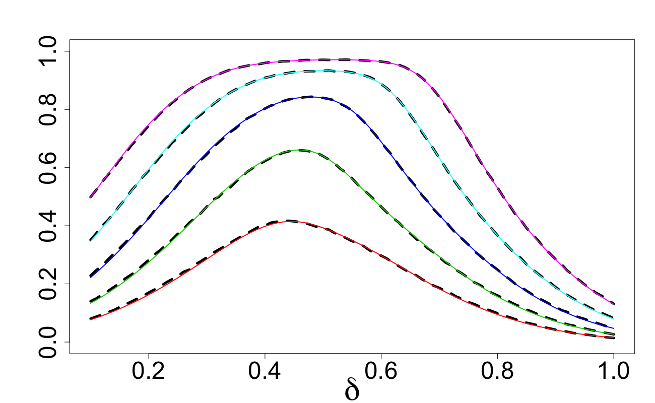
Figure 7: $C_{d}(\mathbb{D}_{n,\delta},r)$ and its approximation: $d=5$, $\\ r$ from $0.7$ to $1.1$ increasing by $0.1$

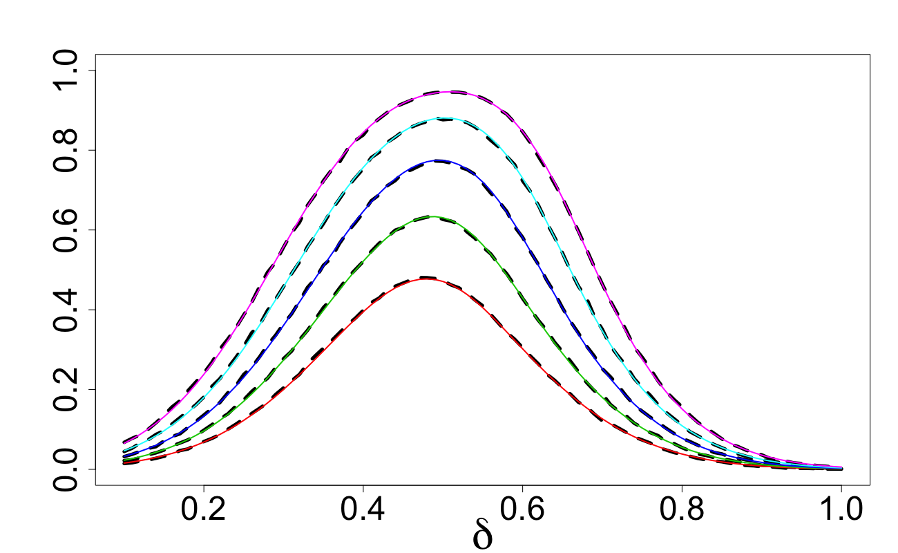
Figure 8: $C_{d}(\mathbb{D}_{n,\delta},r)$ and its approximation: $d=10$, $\\ r$ from $0.95$ to $1.15$ increasing by $0.05$

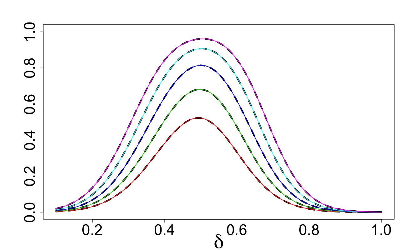
Figure 9: $C_{d}(\mathbb{D}_{n,\delta},r)$ and its approximation: $d=15$, $\\ r$ from $1.15$ to $1.35$ increasing by $0.05$

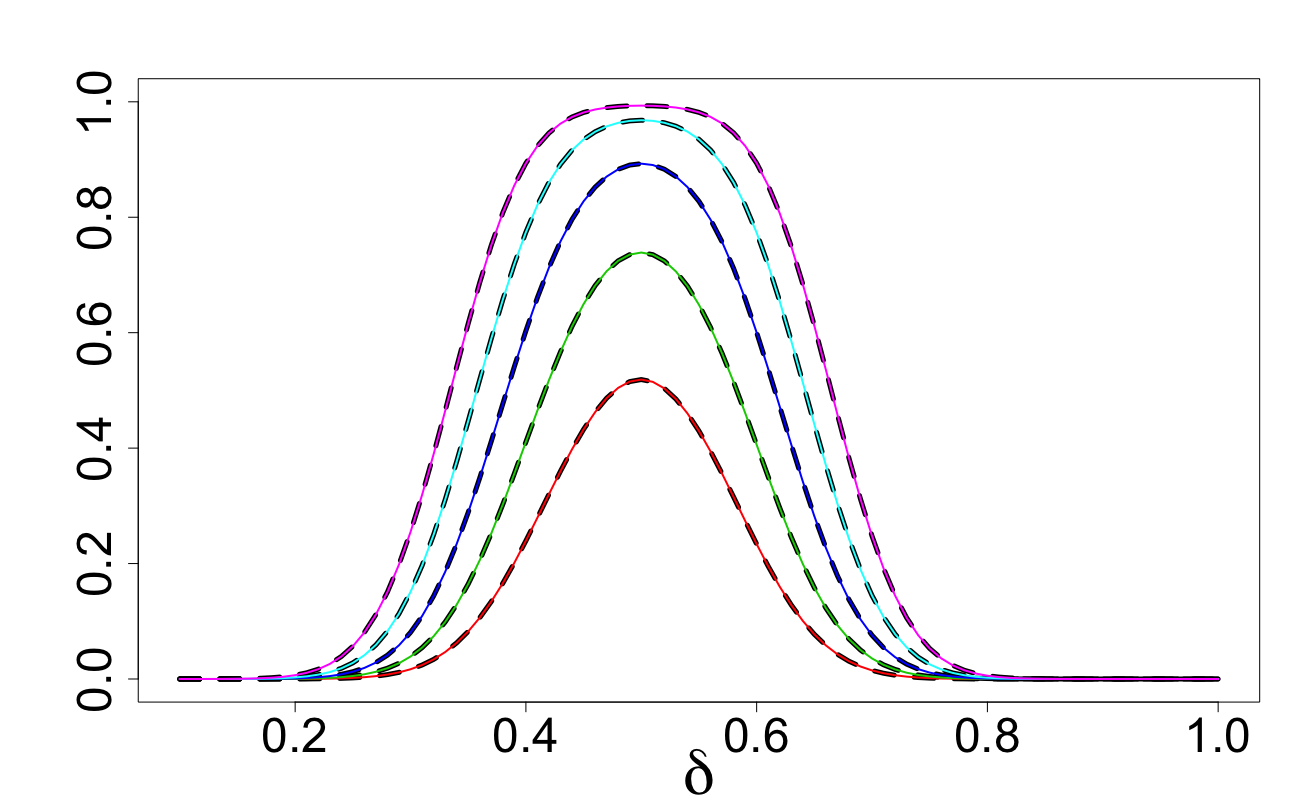
Figure 10: $C_{d}(\mathbb{D}_{n,\delta},r)$ and its approximation: $d=50$, $\\ r$ from $2.05$ to $2.35$ increasing by $0.075$

Figures 12 and 12 illustrate Theorem 3.2 and show the rate of convergence of the covering radii as $d$ increases. Let the probability density function $f(r)$ be defined by $dC_{d}(\mathbb{D}_{n,\delta},r)=f(r)dr$, where $C_{d}(\mathbb{D}_{n,\delta},r)$ as a function of $r$ is viewed as the c.d.f. of the r.v. $r=\varrho(X,\mathbb{Z}_{n})$, see Section 1.3. Trivial calculations yield that the density for the normalised radius $R$ expressed by (5) is $p_{d}(R):={2\sqrt{d}}{n^{-1/d}}f\left({2\sqrt{d}}{n^{-1/d}}R\right)$. In Figure 12, we depict the density $p_{d}(\cdot)$ for $d=5,10$ and $20$ with blue, red and black lines respectively. The respective c.d.f.’s $\int_{0}^{R}p_{d}(\tau)d\tau$ are shown in Figure 12 under the same colouring scheme.

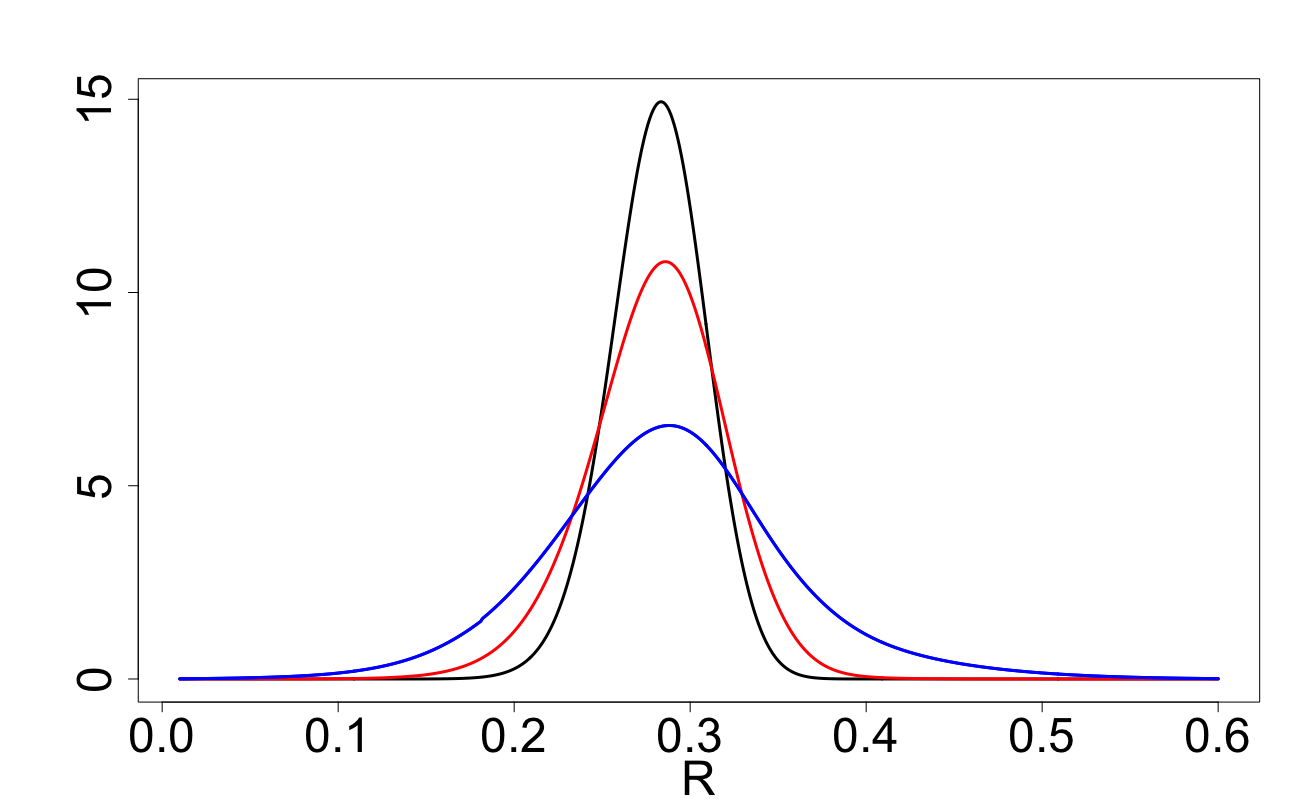
Figure 11: Densities $f_{d}(R)$ for the design $\mathbb{D}_{n,\delta^{\ast}}$ ;
$d=5,10,20$

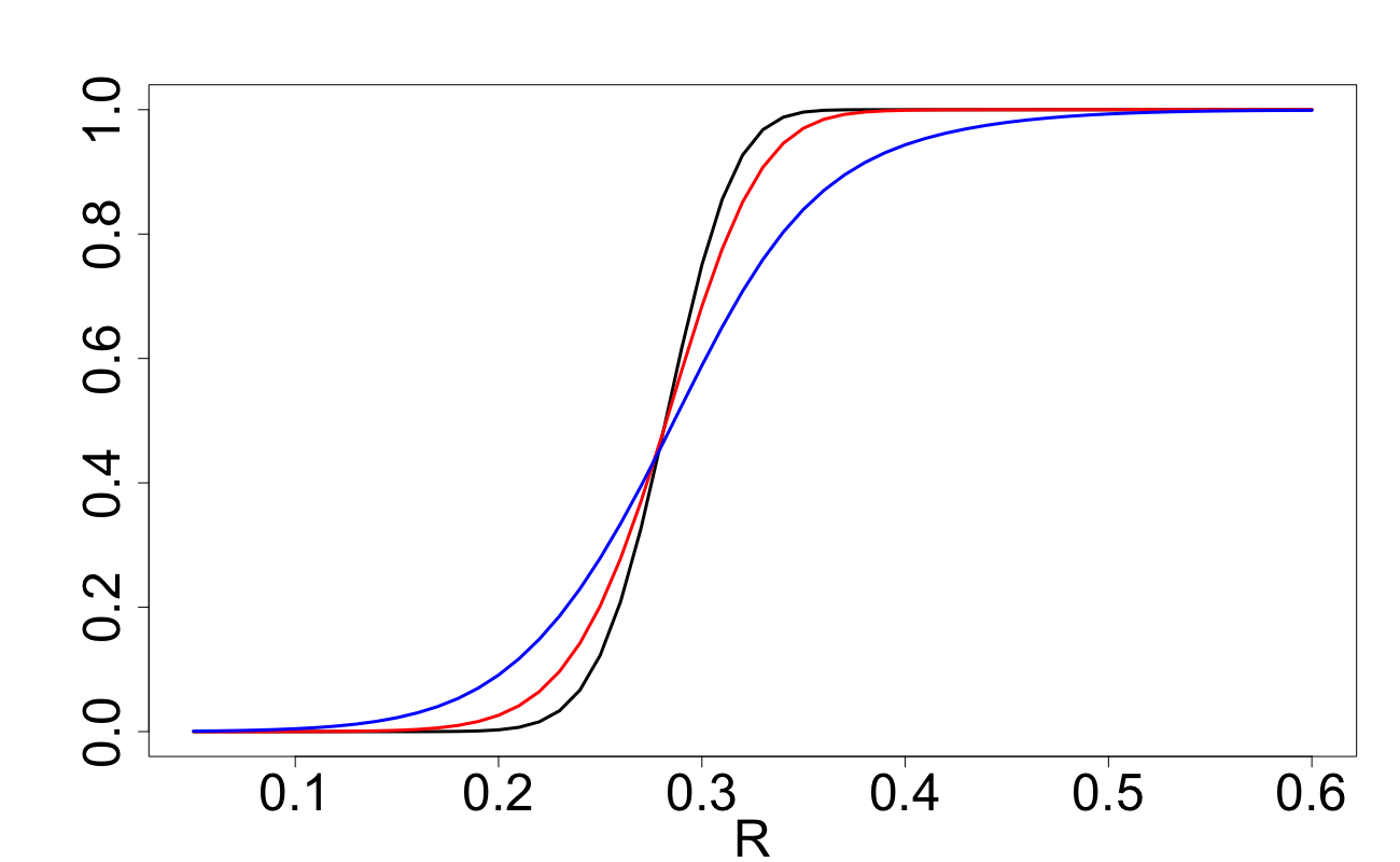
Figure 12: c.d.f.’s of $R$ for the design $\mathbb{D}_{n,\delta^{\ast}}$ ;
$d=5,10,20$

4.3 Stochastic dominance

In Figures 14 and 14, we depict the c.d.f.’s for the normalized distance ${n^{1/d}}\varrho(X,\mathbb{Z}_{n})/({2\sqrt{d}})$ for two designs: $\mathbb{D}_{n,\delta^{\ast}}$ in red, and $\mathbb{D}_{n}^{(0)}$ in black. We can see that the design $\mathbb{D}_{n,\delta^{\ast}}$ stochastically dominates the design $\mathbb{D}_{n}^{(0)}$ for $d=10$ but for $d=5$ the design $\mathbb{D}_{n}^{(0)}$ is preferable to the design $\mathbb{D}_{n,\delta^{\ast}}$ although there is no clear domination; this is in line with findings from Sections 2.4 and 4.1, see e.g. Figure 2, Tables 1 and 2.

In Figure 16, we depict the c.d.f.’s for the normalized distance ${n^{1/d}}\varrho(X,\mathbb{Z}_{n})/({2\sqrt{d}})$ for design $\mathbb{D}_{n}^{(0)}$ (in red) and design $\mathbb{S}_{n}$ (in black). We can see that for $d=5$, the design $\mathbb{D}_{n}^{(0)}$ stochastically dominates the design $\mathbb{S}_{n}$. The style of Figure 16 is the same as figure Figure 16, however we set $d=10$ and the design $\mathbb{D}_{n}^{(0)}$ is replaced with the design $\mathbb{D}_{n,\delta^{\ast}}$. Here we see a very clear stochastic dominance of the design $\mathbb{D}_{n,\delta^{\ast}}$ over the design $\mathbb{S}_{n}$. All findings are consistent with findings from Section 4.1, see Tables 1 and 2.

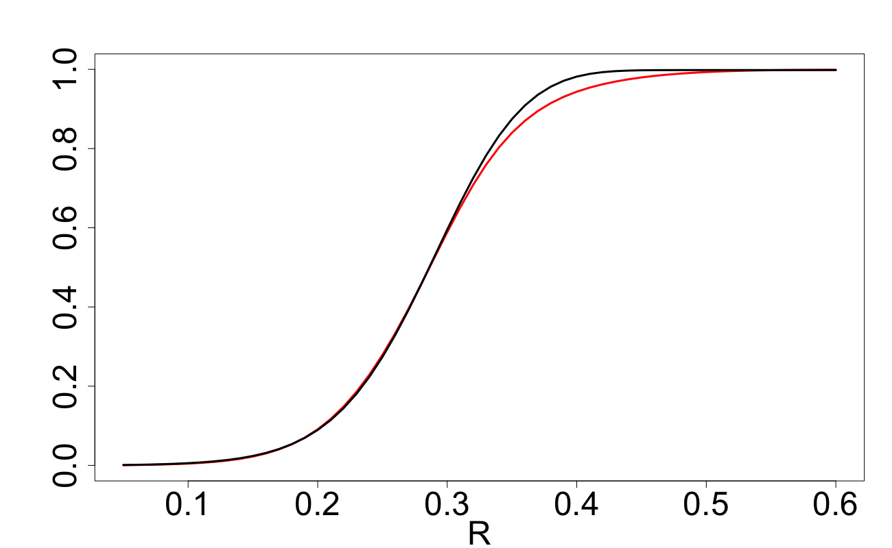
Figure 13: $d=5$: design $\mathbb{D}_{n}^{(0)}$ is preferable to
design $\mathbb{D}_{n,\delta^{\ast}}$

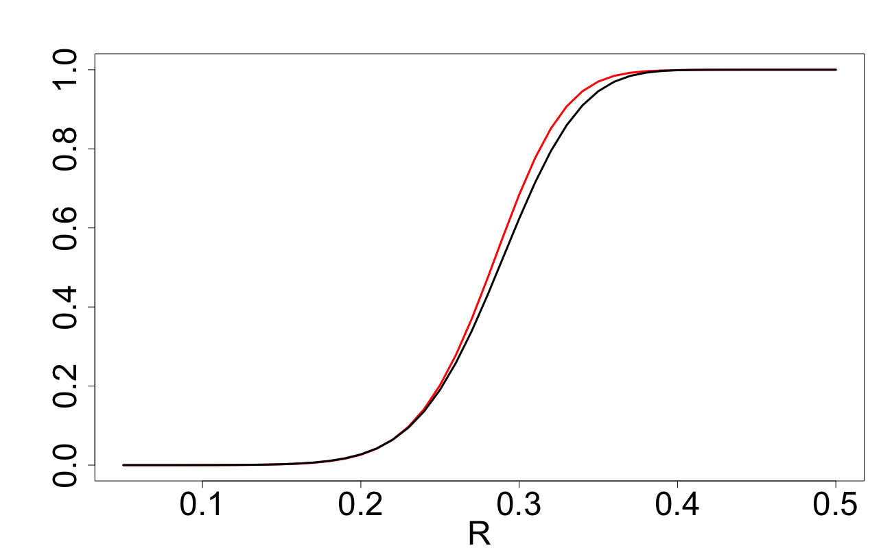
Figure 14: $d=10$: design $\mathbb{D}_{n,\delta^{\ast}}$ stochastically
dominates design $\mathbb{D}_{n}^{(0)}$

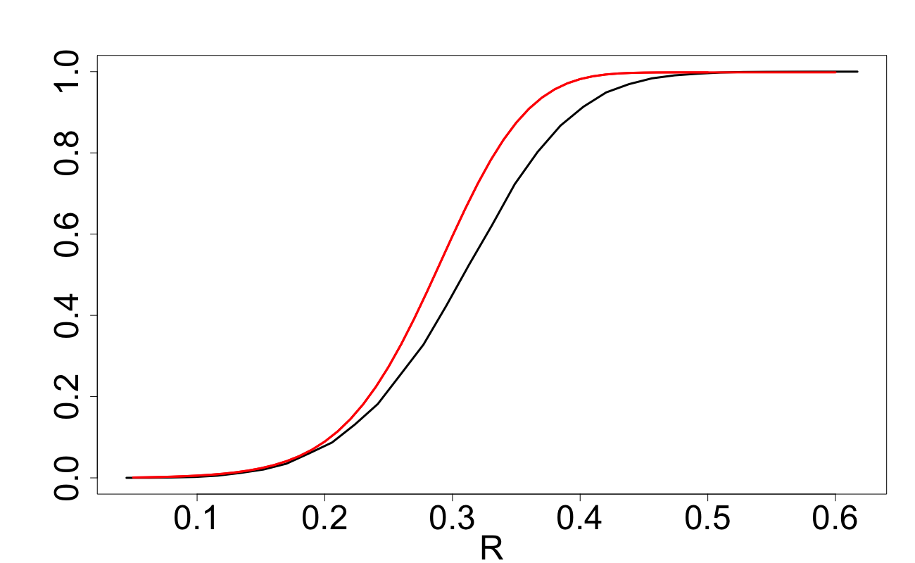
Figure 15: $d=5$: design $\mathbb{D}_{n}^{(0)}$ stochastically
dominates design $\mathbb{S}_{n}$

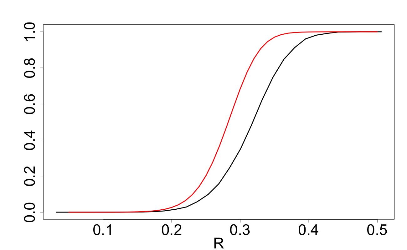
Figure 16: $d=10$: design $\mathbb{D}_{n,\delta^{\ast}}$ stochastically
dominates design $\mathbb{S}_{n}$

Appendix A: Proof of Theorem 3.1

In view of (26), $C_{d}(\mathbb{D}_{n,\delta},r)=V_{d,\boldsymbol{\delta},{r}}$ for all $0\leq\delta\leq 1$ and $r\geq 0$ and we shall derive expressions for $V_{d,\boldsymbol{\delta},{r}}$ rather than $C_{d}(\mathbb{D}_{n,\delta},r)$.

$\mathbf{Case(a):}$ $r\leq\delta$.

To prove this case, we observe i) for this range of $r$, ${\cal B}_{d}(\boldsymbol{\delta},{r})\subset[0,1]^{d}$; ii) the fraction of a cube covered by a ball is preserved under invertible affine transformations; iii) the affine transformation $x\rightarrow 2x-\boldsymbol{1}$ maps the ball ${\cal B}_{d}(\boldsymbol{\delta},{r})$ and cube $[0,1]^{d}$ to ${\cal B}_{d}(\boldsymbol{2\delta-1},{2r})$ and $[-1,1]^{d}$, respectively. This leads to

$$V_{d,\boldsymbol{\delta},{r}}=\frac{{\rm vol}({\cal B}_{d}(\boldsymbol{\delta},{r}))}{2\,{\rm vol}([0,1]^{d})}=\frac{{\rm vol}({\cal B}_{d}(\boldsymbol{2\delta-1},{2r}))}{2\,{\rm vol}([-1,1]^{d})}=\frac{1}{2}C_{d,\boldsymbol{2\delta-1},{2r}}\,.$$

$\mathbf{Case(b)}$: $\delta\leq r\leq 1+\delta$

Using (15) we obtain

$$V_{d,\boldsymbol{\delta},{r}} = \frac{1}{2}\bigg{[}{\rm vol}\left({\cal B}_{d}(\boldsymbol{\delta},{r})\cap C_{0}\right)+d\cdot{\rm vol}\left({\cal B}_{d}(\boldsymbol{\delta},{r})\cap U_{1}\right)\bigg{]}.$$

The first quantity in the brackets has been considered in case (a) and it is simply $C_{d,\boldsymbol{2\delta-1},{2r}}$. Therefore we aim to reformulate the second quantity within the brackets, ${\rm vol}\left({\cal B}_{d}(\boldsymbol{\delta},{r})\cap U_{1}\right)$. Denote by ${\cal P}(t)=\{(x_{1},x_{2},\ldots,x_{d}):x_{1}=t\}$, the $(d-1)$-dimensional hyperplane. Then

$${\rm vol}\left({\cal B}_{d}(\boldsymbol{\delta},{r})\cap U_{1}\right)=\int_{\delta-r}^{0}{\rm vol}_{d-1}({\cal P}(t)\cap{\cal B}_{d}(\boldsymbol{\delta},{r})\cap U_{1})dt\,.$$

Notice further that

$$\begin{aligned} U_{1}\cap{\cal P}(t)=\{t\}\times[|t|,1]^{d-1},&&\text{ for }-1\leq t\leq 0\\ {\cal B}_{d}(\boldsymbol{\delta},{r})\cap{\cal P}(t)=\{t\}\times{\cal B}_{d-1}\left(\boldsymbol{\delta},{\sqrt{r^{2}-(t-\delta)^{2}}}\right)&&\text{ for }\delta-r\leq t\leq 0,r\geq\delta,\end{aligned}$$ (32)

where $\boldsymbol{\delta}=(\delta,\ldots,\delta)\in\mathbb{R}^{d-1}$ and the natural identification of ${\cal P}(t)$ with $\mathbb{R}^{d-1}$ is used. The r.h.s. in (32) are a $(d-1)-$dimensional cube and ball respectively. Since covered fraction is preserved under affine transformations in $\mathbb{R}^{d-1}$, it suffices to construct one, denote by $\phi$, for which $\phi([|t|,1]^{d-1})=[-1,1]^{d}$. In ${\cal P}(t)$, such $\phi$ maps the cube from (32) to the standard cube $[-1,1]^{d}$. Clearly, $\phi$ can be taken as

$$\phi:x\rightarrow\frac{x-(\boldsymbol{1+|t|})/2}{({1-|t|})/2}=\frac{2x-(\boldsymbol{1+|t|})}{{1-|t|}}\,,$$

where ${\boldsymbol{1}}=(1,\ldots,1)$ and $\boldsymbol{|t|}=(|t|,\ldots,|t|)$ are constant vectors in $\mathbb{R}^{d-1}$. Note that,

$$\phi\left({\cal B}_{d-1}\left(\boldsymbol{\delta},{\sqrt{r^{2}-(t-\delta)^{2}}}\right)\right)={\cal B}_{d-1}\left(\frac{\boldsymbol{2\delta-(1+|t|)}}{\boldsymbol{1-|t|}},\frac{2\sqrt{r^{2}-(t-\delta)^{2}}}{1-|t|}\right)\,.$$

Finally, by the preservation of covered fraction, we obtain

$${\rm vol}_{d-1}({\cal P}(t)\cap{\cal B}_{d}(\boldsymbol{\delta},{r})\cap U_{1})={\rm vol}_{d-1}([|t|,1]^{d-1})\cdot C_{d-1,\boldsymbol{\frac{2\delta-1-|{t}|}{1-|{t}|}},{\frac{2\sqrt{r^{2}-(t-\delta)^{2}}}{1-|t|}}}\,.$$

As a result,

$$V_{d,\boldsymbol{\delta},{r}} = \frac{1}{2}\left[C_{d,\boldsymbol{2\delta-1},{2r}}+d\int_{\delta-r}^{0}C_{d-1,\boldsymbol{\frac{2\delta-1-|{t}|}{1-|{t}|}},{\frac{2\sqrt{r^{2}-(t-\delta)^{2}}}{1-|t|}}}(1-|t|)^{d-1}\,dt\right]$$

$$= \frac{1}{2}\left[C_{d,\boldsymbol{2\delta-1},{2r}}+d\int_{0}^{r-\delta}C_{d-1,\boldsymbol{\frac{2\delta-1-{t}}{1-{t}}},{\frac{2\sqrt{r^{2}-(t+\delta)^{2}}}{1-t}}}(1-t)^{d-1}\,dt\right]\,.$$

$\mathbf{Case(c)}$: $r\geq 1+\delta$:

Case (c) is almost identical to Case (b), with the only change occurring within the lower limit of integration in (Appendix A: Proof of Theorem 3.1); the lower limit of the integral remains at $-1$ for all $r\geq 1+\delta$. Since the steps are almost identical to Case (b), they are omitted and we simply conclude:

$$V_{d,\boldsymbol{\delta},{r}}=\frac{1}{2}\left[C_{d,\boldsymbol{2\delta-1},{2r}}+d\int_{0}^{1}C_{d-1,\boldsymbol{\frac{2\delta-1-{t}}{1-{t}}},{\frac{2\sqrt{r^{2}-(t+\delta)^{2}}}{1-t}}}(1-t)^{d-1}\,dt\right]\,.$$

$\Box$

Appendix B: Proof of Lemma 2

(a) Let us first prove the upper bound in (31). Consider the set $U_{j}$ defined in (16) and the associated set

$$U_{j}^{\prime}=\left\{X=(x_{1},x_{2},\ldots,x_{d})\!\in\![0,1]^{d}\!:|x_{j}|\leq x_{k}\leq 1\;\mbox{ \rm for all }k\neq j\right\}\subset C_{0}\,.$$

We have vol($U_{j}$)=vol($U_{j}^{\prime}$)$=1/d$ and

$$V(\boldsymbol{\delta})=C_{0}\bigcup\left[\bigcup_{j=1}^{d}U_{j}\right],\;\;\;\bigcup_{j=1}^{d}U_{j}^{\prime}=C_{0}=[0,1]^{d}$$

Let us prove that for any $r\geq 0$ we have vol($U_{j}\cap{\cal B}_{d}(\boldsymbol{\delta},{r})$)$\leq$ vol($U_{j}^{\prime}\cap{\cal B}_{d}(\boldsymbol{\delta},{r})$).

With any point $X=(x_{1},x_{2},\ldots,x_{d})\!\in\!U_{1}^{\prime}$, we associate the point $X^{\prime}=(-x_{1},x_{2},\ldots,x_{d})\!\in\!U_{1}$ by simply changing the sign in the first component. For these two points, we have

$$\|\boldsymbol{\delta}-X\|^{2}=\left(x_{1}-\delta\right)^{2}+\sum_{k=2}^{d}\left(x_{k}-\delta\right)^{2}<\left(-x_{1}-\delta\right)^{2}+\sum_{k=2}^{d}\left(x_{k}-\delta\right)^{2}=\|\boldsymbol{\delta}-X^{\prime}\|^{2}$$

Therefore, $\|\boldsymbol{\delta}-X\|^{2}\leq r\Rightarrow\|\boldsymbol{\delta}-X^{\prime}\|^{2}\leq r$ yielding:

$${\rm vol}(U_{j}\cap{\cal B}_{d}(\boldsymbol{\delta},{r}))\leq{\rm vol}(U_{j}^{\prime}\cap{\cal B}_{d}(\boldsymbol{\delta},{r}))\,.$$ (34)

To prove the upper bound in (31) for all $r$ we must consider two cases: $r\leq\delta$ and $\,r\geq\delta$.

For $r\leq\delta$, we clearly have

$$V_{d,\boldsymbol{\delta},{r}}=\frac{1}{2}C_{d,\boldsymbol{2\delta-1},{2r}}\leq C_{d,\boldsymbol{2\delta-1},{2r}}$$

For $r\geq\delta$,using (34) we have

$$V_{d,\boldsymbol{\delta},{r}} = \frac{1}{2}\bigg{[}{\rm vol}\left({\cal B}_{d}(\boldsymbol{\delta},{r})\cap C_{0}\right)+d\cdot{\rm vol}\left({\cal B}_{d}(\boldsymbol{\delta},{r})\cap U_{1}\right)\bigg{]}$$

$$\leq \frac{1}{2}\bigg{[}{\rm vol}\left({\cal B}_{d}(\boldsymbol{\delta},{r})\cap C_{0}\right)+d\cdot{\rm vol}\left({\cal B}_{d}(\boldsymbol{\delta},{r})\cap U^{\prime}_{1}\right)\bigg{]}$$

$$= {\rm vol}({\cal B}_{d}(\boldsymbol{\delta},{r})\cap C_{0})$$

$$= C_{d,\boldsymbol{2\delta-1},{2r}}$$

and hence the upper bound in (31).

(b) Consider now the lower bound in (31). For $j\geq 2$, with the set $U_{j}$ we now associate the set

$$V_{j}=\left\{\tilde{X}=(x_{1},\ldots,x_{d})\!:-1\leq x_{1}\leq 0,\;0\leq x_{m}\leq 1\;(\mbox{ \rm for }m>1),\;|x_{j}|\leq|x_{k}|\leq 1\;\mbox{ \rm for }k\neq j\right\}\,.$$

With any point $X=(x_{1},x_{2},\ldots,x_{d})\!\in\!U_{j}$ (here $x_{j}$ is negative and $|x_{j}|\leq|x_{k}|\leq 1\;\mbox{ \rm for }k\neq j$) we associate point $\tilde{X}=(-x_{1},x_{2},\ldots,x_{j-1},-x_{j},x_{j+1},\ldots,x_{d})\!\in\!V_{j}$ by changing sign in the first and $j$-the component of $X\in U_{j}$.

Setting without loss of generality $j=2$, we have for these two points:

$$\|\boldsymbol{\delta}-X\|^{2} = \left(x_{1}-\delta\right)^{2}+\left(x_{2}-\delta\right)^{2}+\sum_{k=3}^{d}\left(x_{k}-\delta\right)^{2}$$

$$\leq \left(-x_{1}-\delta\right)^{2}+\left(-x_{2}-\delta\right)^{2}+\sum_{k=3}^{d}\left(x_{k}-\delta\right)^{2}=\|\boldsymbol{\delta}-\tilde{X}\|^{2}\,,$$

where the inequality follows from the inequalities $x_{1}\geq 0$, $x_{2}<0$ and $|x_{2}|<x_{1}$ containing in the definition of $U_{2}$.

Therefore, $\|\boldsymbol{\delta}-\tilde{X}\|^{2}\leq r\Rightarrow\|\boldsymbol{\delta}-{X}\|^{2}\leq r$ implying:

$${\rm vol}(U_{j}\cap{\cal B}_{d}(\boldsymbol{\delta},{r}))\geq{\rm vol}(V_{j}\cap{\cal B}_{d}(\boldsymbol{\delta},{r}))\,.$$ (35)

To prove the lower bound in (31) for all $r$ we must consider two cases: $r\leq\delta$ and $\,r\geq\delta$.

For $r\geq\delta$, using (35) we have

$$V_{d,\boldsymbol{\delta},{r}} = \frac{1}{2}\bigg{[}{\rm vol}\left({\cal B}_{d}(\boldsymbol{\delta},{r})\cap C_{0}\right)+\sum_{i=1}^{d}{\rm vol}\left(({\cal B}_{d}(\boldsymbol{\delta},{r})\cap U_{i})\right)\bigg{]}$$

$$\geq \frac{1}{2}\bigg{[}{\rm vol}\left({\cal B}_{d}(\boldsymbol{\delta},{r})\cap C_{0}\right)+{\rm vol}({\cal B}_{d}(\boldsymbol{\delta},{r})\cap U_{1})+\sum_{i=2}^{d}\left({\cal B}_{d}(\boldsymbol{\delta},{r})\cap V_{i})\right)\bigg{]}$$

$$= \frac{1}{2}\bigg{[}{\rm vol}\left({\cal B}_{d}(\boldsymbol{\delta},{r})\cap C_{0}\right)+{\rm vol}({\cal B}_{d}(\boldsymbol{\delta},{r})\cap C_{1})\bigg{]}\,,$$

where $C_{1}$ is given in (17). To compute ${\rm vol}({\cal B}_{d}(\boldsymbol{\delta},{r})\cap C_{1})$, we shall use a similar technique to the proof of Theorem 3.1. The affine transformation

$$x\rightarrow 2x+(1,-1,-1,\ldots,-1)$$

maps the ball ${\cal B}_{d}(\boldsymbol{\delta},{r})$ and the cube $C_{1}$ to ${\cal B}_{d}({A},{2r})$ and $[-1,1]^{d}$ respectively, where ${A}=\left(2\delta+1,2\delta-1,\ldots,2\delta-1\right)$. Since the fraction of covered volume is preserved under invertible affine transformations, one has

$$\frac{{\rm vol}({\cal B}_{d}(\boldsymbol{\delta},{r})\cap C_{1})}{{\rm vol}(C_{1})}=C_{d,A,2r}$$

and hence we can conclude:

$$V_{d,\boldsymbol{\delta},{r}} \geq \frac{1}{2}\bigg{[}{\rm vol}\left({\cal B}_{d}(\boldsymbol{\delta},{r})\cap C_{0}\right)+{\rm vol}({\cal B}_{d}(\boldsymbol{\delta},{r})\cap C_{1})\bigg{]}$$

$$= \frac{1}{2}\left[C_{d,\boldsymbol{2\delta-1},{2r}}+C_{d,A,2r}\right]\,.$$

For $r\leq\delta$, since ${\rm vol}({\cal B}_{d}(\boldsymbol{\delta},{r})\cap C_{1})=C_{d,A,2r}=0$, we have

$$V_{d,\boldsymbol{\delta},{r}} = \frac{1}{2}\left[C_{d,\boldsymbol{2\delta-1},{2r}}+C_{d,A,2r}\right]\,$$

and hence the lower bound in (31). $\Box$

Appendix C: Proof of Theorem 3.2.

Before proving Theorem 3.2, we prove three auxiliary lemmas.

Lemma 3

Let $r=r_{\alpha,d}=\alpha\sqrt{d}$ with $\alpha\geq 0$ and $Z_{a,b;d}=(a,b,b,\ldots,b)\in\mathbb{R}^{d}$. Then the limit $\lim_{d\to\infty}C_{d,{Z_{a,b;d}},{2r}}$ exists and

$$\lim_{d\to\infty}C_{d,Z_{a,b;d},{2r}}=\begin{cases}0\text{ if }\alpha<\frac{1}{2}\sqrt{\frac{1}{3}+b^{2}}\\ 1/2\text{ if }\alpha=\frac{1}{2}\sqrt{\frac{1}{3}+b^{2}}\\ 1\text{ if }\alpha>\frac{1}{2}\sqrt{\frac{1}{3}+b^{2}}\,\end{cases}$$

Proof. Define

$$t_{\alpha}=\frac{\sqrt{3}(d(4\alpha^{2}-b^{2}-1/3)+b^{2}-a^{2})}{2\sqrt{a^{2}+(d-1)b^{2}+d/15}}\,.$$

As the r.v. $\eta_{z}$ introduced in Appendix D are concentrated on a finite interval, for finite $a$ and $b$ the quantities of $\rho_{a}:=\mathbb{E}(|\eta_{a}-a^{2}-\frac{1}{3}|^{3})$ and $\rho_{b}:=\mathbb{E}(|\eta_{b}-b^{2}-\frac{1}{3}|^{3})$ are bounded. By applying Berry-Esseen theorem (see §2, Chapter 5 in petrov2012sums ) to $C_{d,Z_{a,b},{2r}}$, there exists some constant $C$ such that

$$-\frac{C\cdot\max\{\rho_{a}/\sigma_{a}^{2},\rho_{b}/\sigma_{b}^{2}\}}{\left(\sigma_{a}^{2}+(d-1)\sigma_{b}^{2}\right)^{1/2}}+\Phi\left(t_{\alpha}\right)\leq C_{d,Z_{a,b},{2r}}\leq\Phi\left(t_{\alpha}\right)+\frac{C\cdot\max\{\rho_{a}/\sigma_{a}^{2},\rho_{b}/\sigma_{b}^{2}\}}{\left(\sigma_{a}^{2}+(d-1)\sigma_{b}^{2}\right)^{1/2}}\,,$$

where $\sigma_{a}^{2}={\rm var}(\eta_{a})$ and $\sigma_{b}^{2}={\rm var}(\eta_{b})$. By the squeeze theorem, it is clear that if $4\alpha^{2}-b^{2}-1/3>0$ and hence $\alpha>\frac{1}{2}\sqrt{\frac{1}{3}+b^{2}}$, then $C_{d,Z_{a,b},{2r}}\rightarrow 1$ as $d\rightarrow\infty$. If $\alpha<\frac{1}{2}\sqrt{\frac{1}{3}+b^{2}}$, then $C_{d,Z_{a,b},{2r}}\rightarrow 0$ as $d\rightarrow\infty$. If $\alpha=\frac{1}{2}\sqrt{\frac{1}{3}+b^{2}}$, then $C_{d,Z_{a,b},{2r}}\rightarrow 1/2$ as $d\rightarrow\infty$. $\Box$

Lemma 4

Let $r=\alpha\sqrt{d}$. Then for $\boldsymbol{\delta}=(\delta,\delta,\ldots,\delta)$, we have:

$$\lim_{d\to\infty}V_{d,\boldsymbol{\delta},{r}}=\lim_{d\to\infty}C_{d,\boldsymbol{2\delta-1},{2r}}=\begin{cases}0\text{ if }\alpha<\frac{\sqrt{1/3+(2\delta-1)^{2}}}{2}\\ 1/2\text{ if }\alpha=\frac{\sqrt{1/3+(2\delta-1)^{2}}}{2}\\ 1\text{ if }\alpha>\frac{\sqrt{1/3+(2\delta-1)^{2}}}{2}\,\end{cases}$$

Proof. Using Lemma 3 with $Z_{a,b}=A=\left(2\delta+1,2\delta-1,\ldots,2\delta-1\right)$, we obtain:

$$\lim_{d\to\infty}C_{d,A,{2r}}=\lim_{d\to\infty}C_{d,\boldsymbol{2\delta-1},{2r}}=\begin{cases}0\text{ if }\alpha<\frac{\sqrt{1/3+(2\delta-1)^{2}}}{2}\\ 1/2\text{ if }\alpha=\frac{\sqrt{1/3+(2\delta-1)^{2}}}{2}\\ 1\text{ if }\alpha>\frac{\sqrt{1/3+(2\delta-1)^{2}}}{2}\,\end{cases}$$

By then applying the squeeze theorem to the bounds in Lemma 2 using the fact from Lemma 1 we have $V_{d,\boldsymbol{\delta},{r}}=C_{d}(\mathbb{Z}_{n},r)$, we obtain the result. $\Box$

To determine the value of $r$ that leads to the full coverage, we utilise the following simple lemma.

Lemma 5

For design ${\mathbb{D}_{n,\delta}}$, the smallest value of $r$ that ensures a complete coverage of $[-1,1]^{d}$ satisfies:

$$\lim_{d\rightarrow\infty}\frac{r_{1}}{\sqrt{d}}=\begin{cases}{(1-\delta)}\text{ if }\delta\leq 1/2\\ {\delta}\text{ if }\delta>1/2\end{cases}\,.$$

Proof of Theorem 3.2.

From Lemma 4, it is clear that the smallest $\alpha$ and hence $r$ is attained with $\delta=1/2$. Moreover, Lemma 4 provides:

$$\lim_{d\to\infty}V_{d,\boldsymbol{1/2},{r}}=\lim_{d\to\infty}C_{d,\boldsymbol{0},{2r}}=\begin{cases}0\text{ if }\alpha<\frac{1}{2\sqrt{3}}\\ 1/2\text{ if }\alpha=\frac{1}{2\sqrt{3}}\\ 1\text{ if }\alpha>\frac{1}{2\sqrt{3}}\,\end{cases}$$

meaning for any $0<\gamma<1$, $r_{1-\gamma}=\frac{\sqrt{d}}{2\sqrt{3}}$. By then applying Lemma 5 with $\delta=1/2$, we obtain $r_{1}=\sqrt{d}/2$ and hence $r_{1-\gamma}/r_{1}\rightarrow 1/\sqrt{3}$ as $d\rightarrow\infty.$ $\Box$

Appendix D: Derivation of approximation (30)

Let $U=(u_{1},\ldots,u_{d})$ be a random vector with uniform distribution on $[-1,1]^{d}$ so that $u_{1},\ldots,u_{d}$ are i.i.d.r.v. uniformly distributed on $[-1,1]$. Then for given $Z=(z_{1},\ldots,z_{d})\in\mathbb{R}^{d}$ and any $r>0$,

$$C_{d,Z,{r}}\!=\!\mathbb{P}\left\{\|U\!-\!Z\|\!\leq\!{r}\right\}\!=\!\mathbb{P}\left\{\|U\!-\!Z\|^{2}\leq{r^{2}}\right\}\!=\!\mathbb{P}\left\{\sum_{j=1}^{d}(u_{j}\!-\!z_{j})^{2}\leq{r}^{2}\right\}.\;\;$$

That is, $C_{d,Z,{r}}$, as a function of ${r}$, is the c.d.f. of the r.v. $\|U-Z\|$.

Let $u$ have the uniform distribution on $[-1,1]$ and $z\in\mathbb{R}$. The first three central moments of the r.v. $\eta_{z}=(u-z)^{2}$ can be easily computed:

$$\mathbb{E}\eta_{z}=z^{2}+\frac{1}{3},\;\;{\rm var}(\eta_{z})=\frac{4}{3}\left(z^{2}+\frac{1}{15}\right)\,,\;\;\mu_{z}^{(3)}=E\left[\eta_{z}-E\eta_{z}\right]^{3}=\frac{16}{15}\left(z^{2}+\frac{1}{63}\right)\,.$$ (36)

Consider the r.v. $\|U-Z\|^{2}=\sum_{i=1}^{d}\eta_{z_{j}}=\sum_{j=1}^{d}(u_{j}-z_{j})^{2}\,.$ From (36) and independence of $u_{1},\ldots,u_{d}$, we obtain

$$\mu_{d,Z}=\mathbb{E}\|U-Z\|^{2}=\|Z\|^{2}+\frac{d}{3}\,\;\;{\sigma}_{d,Z}^{2}={\rm var}(\|U-Z\|^{2})=\frac{4}{3}\left(\|Z\|^{2}+\frac{d}{15}\right)\,\;\;\;\;\;\;$$

and

$${\mu}_{d,Z}^{(3)}=\mathbb{E}\left[\|U-Z\|^{2}-\mu_{d,Z}\right]^{3}=\sum_{j=1}^{d}\mu_{z_{j}}^{(3)}=\frac{16}{15}\left(\|Z\|^{2}+\frac{d}{63}\right)\,.\;\;\;\;\;\;$$

If $d$ is large enough then the conditions of the CLT for $\|U-Z\|^{2}$ are approximately met and the distribution of $\|U-Z\|^{2}$ is approximately normal with mean $\mu_{d,Z}$ and variance ${\sigma}_{d,Z}^{2}$. That is, we can approximate $C_{d,Z,{r}}$ by

$$C_{d,Z,{r}}\cong\Phi\left(\frac{{r}^{2}-\mu_{d,Z}}{{\sigma}_{d,Z}}\right)\,,$$ (37)

where $\Phi(\cdot)$ is the c.d.f. of the standard normal distribution:

$$\Phi(t)=\int_{-\infty}^{t}\varphi(v)dv\;\;{\rm with}\;\;\varphi(v)=\frac{1}{\sqrt{2\pi}}e^{-v^{2}/2}\,.$$

The approximation (37) can be improved by using an Edgeworth-type expansion in the CLT for sums of independent non-identically distributed r.v.

General expansion in the central limit theorem for sums of independent non-identical r.v. has been derived by V.Petrov, see Theorem 7 in Chapter 6 in petrov2012sums ; the first three terms of this expansion have been specialized in Section 5.6 in petrov . By using only the first term in this expansion, we obtain the following approximation for the distribution function of $\|U-Z\|^{2}$:

$$P\left(\frac{\|U-Z\|^{2}-\mu_{d,Z}}{\sigma_{d,Z}}\leq x\right)\cong\Phi(x)+\frac{{\mu}_{d,Z}^{(3)}}{6({\sigma}_{d,Z}^{2})^{3/2}}(1-x^{2})\varphi(x),$$

leading to the following improved form of (37):

$$C_{d,Z,{r}}\cong\Phi(t)+\frac{\|Z\|^{2}+d/63}{5\sqrt{3}(\|Z\|^{2}+d/15)^{3/2}}(1-t^{2})\varphi(t)\,,$$

where

$$t=t_{d,\|Z\|,{r}}=\frac{{r}^{2}-\mu_{d,Z}}{{\sigma}_{d,Z}}=\frac{\sqrt{3}(r^{2}-\|Z\|^{2}-d/3)}{2\sqrt{\|Z\|^{2}+{d}/{15}}}\,.$$

- [1] L. Pronzato and W. Müller. Design of computer experiments: space filling and beyond. Statistics and Computing, 22(3):681–701, 2012.
- [2] L. Pronzato. Minimax and maximin space-filling designs: some properties and methods for construction. Journal de la Société Française de Statistique, 158(1):7–36, 2017.
- [3] T. Santner, B. Williams, W. Notz, and B. Williams. The design and analysis of computer experiments. Springer, 2003.
- [4] A. Zhigljavsky and A. Žilinskas. Bayesian and High-Dimensional Global Optimization. Springer, 2021.
- [5] R. Schaback and H. Wendland. Kernel techniques: from machine learning to meshless methods. Acta Numerica, 15:543–639, 2006.
- [6] H. Wendland. Scattered Data Approximation. Cambridge University Press, 2005.
- [7] L. Pronzato and A. Zhigljavsky. Bayesian quadrature, energy minimization, and space-filling design. SIAM/ASA Journal on Uncertainty Quantification, 8(3):959–1011, 2020.
- [8] J. Conway and N. Sloane. Sphere packings, lattices and groups. Springer Science & Business Media, 2013.
- [9] J. Noonan and A. Zhigljavsky. Covering of high-dimensional cubes and quantization. SN Operations Research Forum, 1(3):1–32, 2020.
- [10] J. Noonan and A. Zhigljavsky. Non-lattice covering and quantization in high dimensions. In Black Box Optimization, Machine Learning and No-Free Lunch Theorems, pages 799–860. Springer, 2021.
- [11] S. Graf and H. Luschgy. Foundations of quantization for probability distributions. Springer, 2007.
- [12] Y. Saka, M. Gunzburger, and J. Burkardt. Latinized, improved LHS, and CVT point sets in hypercubes. International Journal of Numerical Analysis and Modeling, 4(3-4):729–743, 2007.
- [13] F. Kuo, S. Joe, M. Matsumoto, S. Mori, and M. Saito. Sobol Sequences with Better Two-Dimensional Projections. https://CRAN.R-project.org/package=SobolSequence, 2017.
- [14] V. Petrov. Sums of independent random variables. Springer-Verlag, 1975.
- [15] V. Petrov. Limit theorems of probability theory: sequences of independent random variables. Oxford Science Publications, 1995.