Transforming variables to central normality

Abstract

Many real data sets contain numerical features (variables) whose distribution is far from normal (gaussian). Instead, their distribution is often skewed. In order to handle such data it is customary to preprocess the variables to make them more normal. The Box-Cox and Yeo-Johnson transformations are well-known tools for this. However, the standard maximum likelihood estimator of their transformation parameter is highly sensitive to outliers, and will often try to move outliers inward at the expense of the normality of the central part of the data. We propose a modification of these transformations as well as an estimator of the transformation parameter that is robust to outliers, so the transformed data can be approximately normal in the center and a few outliers may deviate from it. It compares favorably to existing techniques in an extensive simulation study and on real data.

Keywords: Anomaly detection, Data preprocessing, Feature transformation, Outliers, Symmetrization.

1 Introduction

In machine learning and statistics, some numerical data features may be very nonnormal (nongaussian) and asymmetric (skewed) which often complicates the next steps of the analysis. Therefore it is customary to preprocess the data by transforming such features in order to bring them closer to normality, after which it typically becomes easier to fit a model or to make predictions. To be useful in practice, it must be possible to automate this preprocessing step.

In order to transform a positive variable to give it a more normal distribution one often resorts to a power transformation (see e.g. [17]). The most often used function is the Box-Cox (BC) power transform $g_{\lambda}$ studied by [4], given by

$$g_{\lambda}(x)=\begin{cases}(x^{\lambda}-1)/\lambda&\mbox{ if }\lambda\neq 0\\ \log(x)&\mbox{ if }\lambda=0.\end{cases}$$ (1)

Here $x$ stands for the observed feature, which is transformed to $g_{\lambda}(x)$ using a parameter $\lambda$. A limitation of the family of BC transformations is that they are only applicable to positive data. To remedy this, Yeo and Johnson [22] proposed an alternative family of transformations that can deal with both positive and negative data. These Yeo-Johnson (YJ) transformations $h_{\lambda}$ are given by

$$h_{\lambda}(x)=\begin{cases}((1+x)^{\lambda}-1)/\lambda&\mbox{ if }\lambda\neq 0\mbox{ and }x\geq 0\\ \log(1+x)&\mbox{ if }\lambda=0\mbox{ and }x\geq 0\\ -((1-x)^{2-\lambda}-1)/(2-\lambda)&\mbox{ if }\lambda\neq 2\mbox{ and }x<0\\ -\log(1-x)&\mbox{ if }\lambda=2\mbox{ and }x<0\end{cases}$$ (2)

and are also characterized by a parameter $\lambda$. Figure 1 shows both of these transformations for a range of $\lambda$ values. In both families $\lambda=1$ yields a linear relation. Transformations with $\lambda<1$ compress the right tail of the distribution while expanding the left tail, making them suitable for transforming right-skewed distributions towards symmetry. Similarly, transformations with $\lambda>1$ are designed to make left-skewed distributions more symmetrical.

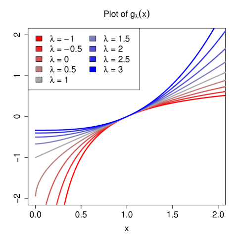
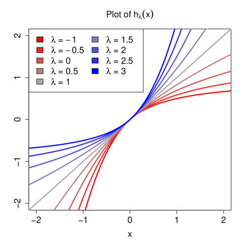
Figure 1: The Box-Cox (left) and Yeo-Johnson (right) transformations for several parameters $\lambda$.

Estimating the parameter $\lambda$ for the BC or YJ transformation is typically done using maximum likelihood, under the assumption that the transformed variable follows a normal distribution. However, it is well known that maximum likelihood estimation is very sensitive to outliers in the data, to the extent that a single outlier can have an arbitrarily large effect on the estimate. In the setting of transformation to normality, outliers can yield transformations for which the bulk of the transformed data follows a very skewed distribution, so no normality is attained at all. In situations with outliers one would prefer to make the non-outliers approximately normally distributed, while the outliers may stay outlying. So, our goal is to achieve central normality, where the transformed data look roughly normal in the center and a few outliers may deviate from it. Fitting such a transformation is not easy, because a point that is outlying in the original data may not be outlying in the transformed data, and vice versa. The problem is that we do not know beforehand which points may turn out to be outliers in the optimally transformed data.

Some proposals exist in the literature to make the estimation of the parameter $\lambda$ in BC more robust against outliers, mainly in the context of transforming the response variable in a regression ([5, 12, 15]), but here we are not in that setting. For the YJ transformation very few robust methods are available. In [18] a trimmed maximum likelihood approach was explored, in which the objective is a trimmed sum of log likelihoods in which the lowest terms are discarded. We will study this method in more detail later.

Note that both the BC and YJ transformations suffer from the complication that their range depends on the parameter $\lambda$. In particular, for the BC transformation we have

$$g_{\lambda}(\mathbb{R}_{0}^{+})=\begin{cases}(-1/|\lambda|,\infty)&\mbox{ if }\lambda>0\\ \mathbb{R}&\mbox{ if }\lambda=0\\ (-\infty,1/|\lambda|)&\mbox{ if }\lambda<0\end{cases}$$ (3)

whereas for the YJ transformation we have

$$h_{\lambda}(\mathbb{R})=\begin{cases}(-1/|\lambda-2|,\infty)&\mbox{ if }\lambda>2\\ \mathbb{R}&\mbox{ if }0\leq\lambda\leq 2\\ (-\infty,1/|\lambda|)&\mbox{ if }\lambda<0.\end{cases}$$ (4)

So, for certain values of $\lambda$ the range of the transformation is a half line. This is not without consequences. First, most well-known symmetric distributions are supported on the entire line, so a perfect match is impossible. More importantly, we argue that this can make outlier detection more difficult. Consider for instance the BC transformation with $\lambda=-1$ which has the range $g_{-1}(\mathbb{R}_{0}^{+})=(-\infty,1)$. Suppose we transform a data set $(x_{1},\ldots,x_{n})$ to $(g_{-1}(x_{1}),\ldots,g_{-1}(x_{n}))$. If we let $x_{n}\to\infty$ making it an extremely clear outlier in the original space, then $g_{-1}(x_{n})\to 1$ in the transformed space. So a transformed outlier can be much closer to the bulk of the transformed data than the original outlier was in the original data. This is undesirable, since the outlier will be much harder to detect this way. This effect is magnified if $\lambda$ is estimated by maximum likelihood, since this estimator will try to accommodate all observations, including the outliers.

We illustrate this point using the TopGear dataset [1] which contains information on 297 cars, scraped from the website of the British television show Top Gear. We fit a Box-Cox transformation to the variable miles per gallon (MPG) which is strictly positive. The left panel of Figure 2 shows the normal QQ-plot of the MPG variable before transformation. (That is, the horizontal axis contains as many quantiles from the standard normal distribution as there are sorted data values on the vertical axis.) In this plot the majority of the observations seem to roughly follow a normal distribution, that is, many points in the QQ-plot lie close to a straight line. There are also three far outliers at the top, which correspond to the Chevrolet Volt and Vauxhall Ampera (both with 235 MPG) and the BMW i3 (with 470 MPG). These cars are unusual because they derive most of their power from a plug-in electric battery, whereas the majority of the cars in the data set are gas-powered. The right panel of Figure 2 shows the Box-Cox transformed data using the maximum likelihood (ML) estimate $\hat{\lambda}=-0.11$, indicating that the BC transformation is fairly close to the log transform. We see that this transformation does not improve the normality of the MPG variable. Instead it tries to bring the three outliers into the fold, at the expense of causing skewness in the central part of the transformed data and creating an artificial outlier at the bottom.

Figure 2: Normal QQ-plot of the variable MPG in the Top Gear dataset (left) and the Box-Cox transformed variable using the maximum likelihood estimate of $\lambda$ (right). The ML estimate is heavily affected by the three outliers at the top, causing it to create skewness in the central part of the transformed data.

The variable Weight shown in Figure 3 illustrates a different effect. The original variable has one extreme and 4 intermediate outliers at the bottom. The extreme outlier is the Peugeot 107, whose weight was erroneously listed as 210 kilograms, and the next outlier is the tiny Renault Twizy (410 kilograms). Unlike the MPG variable the central part of these data is not very normal, as those points in the QQ-plot do not line up so well. A transform that would make the central part more straight would expose the outliers at the bottom more. But instead the ML estimate is $\hat{\lambda}=0.83$ hence close to $\lambda=1$ which would correspond to not transforming the variable at all. Whereas the MPG variable should not be transformed much but is, the Weight variable should be transformed but almost isn’t.

Figure 3: Normal QQ-plot of the variable Weight in the Top Gear dataset (left) and the transformed variable using the ML estimate of $\lambda$ (right). The transformation does not make the five outliers at the bottom stand out.

In section 2 we propose a new robust estimator for the parameter $\lambda$, and compare its sensitivity curve to those of other methods. Section 3 presents a simulation to study the performance of several estimators on clean and contaminated data. Section 4 illustrates the proposed method on real data examples, and section 6 concludes.

2 Methodology

2.1 Fitting a transformation by minimizing a robust criterion

The most popular way of estimating the $\lambda$ of the BC and YJ transformations is to use maximum likelihood (ML) under the assumption that the transformed variable follows a normal distribution, as will briefly be summarized in subsection 2.3. However, it is well known that ML estimation is very sensitive to outliers in the data and other deviations from the assumed model. We therefore propose a different way of estimating the transformation parameter of a transformation.

Consider an ordered sample of univariate observations $X=(x_{(1)},\ldots,x_{(n)})$ and a symmetric target distribution $F$. Suppose we want to estimate the parameter $\lambda$ of a nonlinear function $g_{\lambda}$ such that $g_{\lambda}(x_{(1)}),\ldots,g_{\lambda}(x_{(n)})$ come close to quantiles from the standard normal cumulative distribution function $\Phi$. We propose to estimate $\lambda$ as:

$$\hat{\lambda}=\operatorname*{\mbox{argmin}}_{\lambda}\;\sum_{i=1}^{n}{\rho\left(\frac{g_{\lambda}(x_{(i)})-\hat{\mu}_{\mbox{\tiny{M}}}}{\hat{\sigma}_{\mbox{\tiny{M}}}}-\Phi^{-1}(p_{i})\right)}\;.$$ (5)

Here $\hat{\mu}_{\mbox{\tiny{M}}}$ is the Huber M-estimate of location of the $g_{\lambda}(x_{(i)})$, and $\hat{\sigma}_{\mbox{\tiny{M}}}$ is their Huber M-estimate of scale. Both are standard robust univariate estimators (see [8]). The $p_{i}=(i-1/3)/(n+1/3)$ are the usual equispaced probabilities that also yield the quantiles in the QQ-plot (see, e.g., page 225 in [7]). The function $\rho$ needs to be positive, even and continuously differentiable. In least squares methods $\rho(t)=t^{2}$, but in our situation there can be large absolute residuals $|\frac{g_{\lambda}(x_{(i)})-\hat{\mu}}{\hat{\sigma}}-\Phi^{-1}(p_{i})|$ caused by outlying values of $g_{\lambda}(x_{(i)})$. In order to obtain a robust method we need a bounded $\rho$ function. We propose to use the well-known Tukey bisquare $\rho$-function given by

$$\rho_{\mbox{\small{bw}}}(x)=\begin{cases}1-(1-(x/c)^{2})^{3}&\mbox{ if }|x|\leq c\\ 1&\mbox{ if }|x|>c\,.\end{cases}$$ (6)

The constant $c$ is a tuning parameter, which we set to 0.5 by default here. See section A of the supplementary material for a motivation of this choice.

To calculate $\hat{\lambda}$ numerically, we use the R function optimize() which relies on a combination of golden section search and successive parabolic interpolation to minimize the objective of (5).

2.2 Rectified Box-Cox and Yeo-Johnson transformations

In this section we propose a modification of the classical BC and YJ transformations, called the rectified BC and YJ transformations. They make a continuously differentiable switch to a linear transformation in the tails of the BC and YJ functions. The purpose of these modified transformations is to remedy two issues. First, the range of the classical BC and YJ transformations depends on $\lambda$ and is often only a half line. And second, as argued in the introduction, the classical transformations often push outliers closer to the majority of the data, which makes the outliers harder to detect. Instead the range of the proposed modified transformations is always the entire real line, and it becomes less likely that outliers are masked by the transformation.

For $\lambda<1$, the BC transformation is designed to make right-skewed distributions more symmetrical, and is bounded from above. In this case we define the rectified BC transformation as follows. Consider an upper constant $C_{u}>1$. The rectified BC transformation $\mathring{g}_{\lambda}$ is defined as

$$\mathring{g}_{\lambda}(x)=\begin{cases}g_{\lambda}(x)&\mbox{ if }x\leq C_{u}\\ g_{\lambda}(C_{u})+(x-C_{u})g_{\lambda}^{\prime}(C_{u})&\mbox{ if }x>C_{u}\,.\end{cases}$$ (7)

Similarly, for $\lambda>1$ and a positive lower constant $C_{\ell}<1$ we put

$$\mathring{g}_{\lambda}(x)=\begin{cases}g_{\lambda}(C_{\ell})+(x-C_{\ell})g_{\lambda}^{\prime}(C_{\ell})&\mbox{ if }x<C_{\ell}\\ g_{\lambda}(x)&\mbox{ if }x\geq C_{\ell}\,.\end{cases}$$ (8)

For the YJ transformation we construct rectified counterparts in a similar fashion. For $\lambda<1$ and a value $C_{u}>0$ we define the rectified YJ transformation $\mathring{h}_{\lambda}(x)$ as in (7) with $g_{\lambda}$ replaced by $h_{\lambda}$:

$$\mathring{h}_{\lambda}(x)=\begin{cases}h_{\lambda}(x)&\mbox{ if }x\leq C_{u}\\ h_{\lambda}(C_{u})+(x-C_{u})h_{\lambda}^{\prime}(C_{u})&\mbox{ if }x>C_{u}\,.\end{cases}$$ (9)

Analogously, for $\lambda>1$ and $C_{\ell}<0$ we define $\mathring{h}_{\lambda}(x)$ as in (8):

$$\mathring{h}_{\lambda}(x)=\begin{cases}h_{\lambda}(C_{\ell})+(x-C_{\ell})h_{\lambda}^{\prime}(C_{\ell})&\mbox{ if }x<C_{\ell}\\ h_{\lambda}(x)&\mbox{ if }x\geq C_{\ell}\,.\end{cases}$$ (10)

Figure 4 shows such rectified BC and YJ transformations.

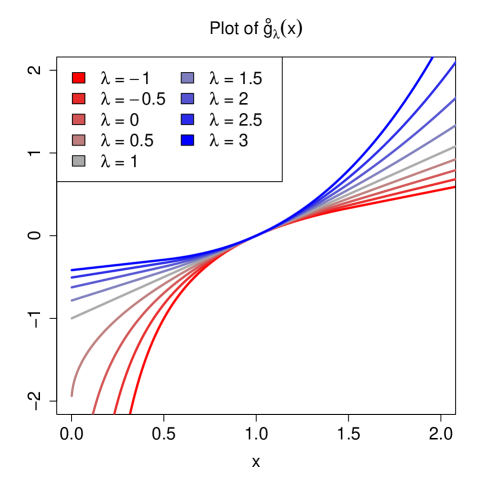
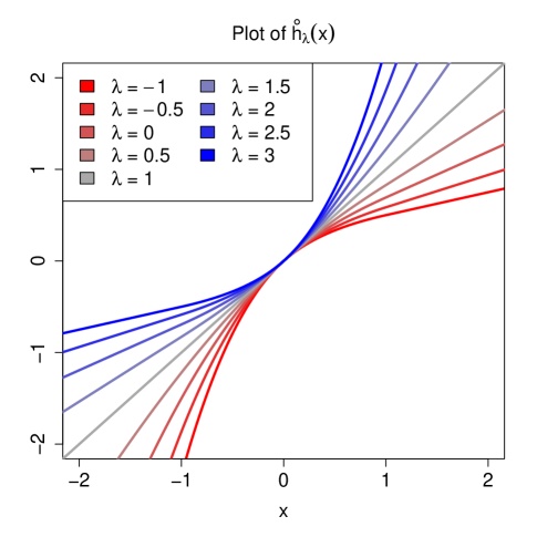
Figure 4: The rectified Box-Cox (left) and Yeo-Johnson (right) transformations for a range of parameters $\lambda$. They look quite similar to the original transformations in Figure 1 but contract less on the right when $\lambda<1$, and contract less on the left when $\lambda>1$.

What are good choices of $C_{\ell}$ and $C_{u}$? Since the original data is often asymmetric, we cannot just use a center (like the median) plus or minus a fixed number of (robust) standard deviations. Instead we set $C_{\ell}$ equal to the first quartile of the original data, and for $C_{u}$ we take the third quartile. Other choices could be used, but more extreme quantiles would yield a higher sensitivity to outliers.

2.3 Reweighted maximum likelihood

We now describe a reweighting scheme to increase the accuracy of the estimated $\hat{\lambda}$ while preserving its robustness. For a data set $x_{1},\ldots,x_{n}$ the classical maximum likelihood estimator for the Yeo-Johnson transformation parameter $\lambda$ is given by the $\lambda$ which maximizes the normal loglikelihood. After removing constant terms this can be written as:

$$\hat{\lambda}_{\mbox{\tiny{ML}}}^{\mbox{\tiny{YJ}}}=\operatorname*{\mbox{argmax}}_{\lambda}\;{\sum_{i=1}^{n}{-\frac{1}{2}\log(\hat{\sigma}_{\mbox{\tiny{ML}},\lambda}^{2})+(\lambda-1)\operatorname{sign}(x_{i})\log(|x_{i}|+1)}}$$ (11)

where $\hat{\sigma}_{\mbox{\tiny{ML}},\lambda}^{2}$ is the maximum likelihood scale of the transformed data given by

$$\hat{\sigma}_{\mbox{\tiny{ML}},\lambda}^{2}=\frac{1}{n}\sum_{i=1}^{n}{(h_{\lambda}(x_{i})-\hat{\mu}_{\mbox{\tiny{ML}},\lambda})^{2}}\quad\mbox{where}\quad\hat{\mu}_{\mbox{\tiny{ML}},\lambda}=\frac{1}{n}\sum_{i=1}^{n}{h_{\lambda}(x_{i})}\;.$$ (12)

The last term in (11) comes from the derivative of the YJ transformation. Criterion (11) is sensitive to outliers since it depends on a classical variance and the unbounded term $\log(1+|x_{i}|)$. This can be remedied by using weights. Given a set of weights $W=(w_{1},\ldots,w_{n})$ we define a weighted maximum likelihood (WML) estimator by

$$\hat{\lambda}_{\mbox{\tiny{WML}}}^{\mbox{\tiny{YJ}}}=\operatorname*{\mbox{argmax}}_{\lambda}\;{\sum_{i=1}^{n}{w_{i}\left[-\frac{1}{2}\log(\hat{\sigma}_{\mbox{\tiny{W}},\lambda}^{2})+(\lambda-1)\operatorname{sign}(x_{i})\log(1+|x_{i}|)\right]}}$$ (13)

where $\hat{\sigma}_{\mbox{\tiny{W}},\lambda}^{2}$ now denotes the weighted variance of the transformed data:

$$\hat{\sigma}_{\mbox{\tiny{W}},\lambda}^{2}=\frac{\sum_{i=1}^{n}{w_{i}(h_{\lambda}(x_{i})-\hat{\mu}_{\mbox{\tiny{W}},\lambda})^{2}}}{\sum_{i=1}^{n}{w_{i}}}\quad\mbox{where}\quad\hat{\mu}_{\mbox{\tiny{W}},\lambda}=\frac{\sum_{i=1}^{n}{w_{i}\,h_{\lambda}(x_{i})}}{\sum_{i=1}^{n}{w_{i}}}\;.$$ (14)

If the weights appropriately downweight the outliers in the data, the WML criterion yields a more robust estimate of the transformation parameter.

For the BC transform the reasoning is analogous, the only change being the final term that comes from the derivative of the BC transform. This yields

$$\hat{\lambda}_{\mbox{\tiny{WML}}}^{\mbox{\tiny{BC}}}=\operatorname*{\mbox{argmax}}_{\lambda}\;{\sum_{i=1}^{n}{w_{i}\left[-\frac{1}{2}\log(\hat{\sigma}_{\mbox{\tiny{W}},\lambda}^{2})+(\lambda-1)\log(x_{i})\right]}}\;\;.$$ (15)

In general, finding robust data weights is not an easy task. The problem is that the observed data $X=(x_{1},\ldots,x_{n})$ can have a (very) skewed distribution and there is no straightforward way to know which points will be outliers in the transformed data when $\lambda$ is unknown. But suppose that we have a rough initial estimate $\lambda_{0}$ of $\lambda$. We can then transform the data with $\lambda_{0}$ yielding $h_{\lambda_{0}}(X)=(h_{\lambda_{0}}(x_{1}),\ldots,h_{\lambda_{0}}(x_{n}))$, which should be a lot more symmetric than the original data. We can therefore compute weights on $h_{\lambda_{0}}(X)$ using a classical weight function. Here we will use the ”hard rejection rule” given by

$$w_{i}=\begin{cases}1&\mbox{ if }|h_{\lambda_{0}}(x_{i})-\hat{\mu}|\leqslant\Phi^{-1}(0.995)\,\hat{\sigma}\\ 0&\mbox{ if }|h_{\lambda_{0}}(x_{i})-\hat{\mu}|>\Phi^{-1}(0.995)\,\hat{\sigma}\\ \end{cases}$$ (16)

with $\hat{\mu}$ and $\hat{\sigma}$ as in (5). With these weights we can compute a reweighted estimate $\hat{\lambda}_{1}$ by the WML estimator in (13). Of course, the robustness of the reweighted estimator will depend strongly on the robustness of the initial estimate $\lambda_{0}$ .

Note that the reweighting step can be iterated, yielding a multistep weighted ML estimator. In simulation studies we found that more than 2 reweighting steps provided no further improvement in terms of accuracy (these results are not shown for brevity). We will always use two reweighting steps from here onward.

2.4 The proposed method

Combining the above ideas, our proposed reweighted maximum likelihood (RewML) method consists of the following steps:

• Step 1. Compute the initial estimate $\lambda_{0}$ by maximizing the robust criterion (5). When fitting a Box-Cox transformation, plug in the rectified function $\mathring{g}_{\lambda}$. When fitting a Yeo-Johnson transformation, use the rectified function $\mathring{h}_{\lambda}$. Note that the rectified transforms are only used in this first step.

• Step 2. Using $\lambda_{0}$ as starting value, compute the reweighted ML estimate from (15) when fitting the unrectified Box-Cox transform $g_{\lambda}$ , and from (13) when fitting the unrectified Yeo-Johnson transform $h_{\lambda}$ .

• Step 3. Repeat step 2 once and stop.

2.5 Other estimators of $\lambda$

We will compare our proposal with two existing robust methods.

The first is the robustified ML estimator proposed by Carroll in 1980 ([5]). The idea was to replace the variance $\hat{\sigma}_{\mbox{\tiny{ML}},\lambda}^{2}$ in the ML formula (11) by a robust variance estimate of the transformed data. Carroll’s method was proposed for the BC transformation, but the idea can be extended naturally to the estimation of the parameter of the YJ transformation. The estimator is then given by

$$\hat{\lambda}_{\mbox{Carroll}}=\operatorname*{\mbox{argmax}}_{\lambda}\;{\sum_{i=1}^{n}{-\frac{1}{2}\log(\hat{\sigma}_{\text{M},\lambda}^{2})+(\lambda-1)\operatorname{sign}(x_{i})\log(1+|x_{i}|)}}$$ (17)

where $\hat{\sigma}_{\text{M},\lambda}$ denotes the usual Huber M-estimate of scale [8] of the transformed data set $(h_{\lambda}(x_{1}),\ldots,h_{\lambda}(x_{n}))$.

The second method is the maximum trimmed likelihood (MTL) estimator of [18]. Given a data set of size $n$, and a fixed number $h$ that has to satisfy $\lceil\frac{n}{2}\rceil<h<n$, this method looks for the parameter $\hat{\lambda}$ which produces a subset of $h$ consecutive observations which maximize the ML criterion (11).

2.6 Sensitivity curves

In order to assess robustness against an outlier, stylized sensitivity curves were introduced on page 96 of [2]. For a given estimator $T$ and a cumulative distribution function $F$ they are constructed as follows:

1. Generate a stylized pseudo data set $X^{0}$ of size $n-1$:

   $$X^{0}=(x_{1},\ldots,x_{n-1})=\left(F^{-1}(p_{1}),\ldots,F^{-1}(p_{n-1})\right)$$

   where the $p_{i}$ for $i,\ldots,n-1$ are equispaced probabilities that are symmetric about 1/2. We can for instance use $p_{i}=i/n$.

2. Add to this stylized data set a variable point $z$ to obtain

   $$X_{z}=(x_{1},\ldots,x_{n-1},z).$$

3. Calculate the sensitivity curve in $z$ by

   $$\mbox{SC}_{n}(z)\coloneqq n\left(T(X_{z})-T(X^{0})\right)$$

   where $z$ ranges over a grid chosen by the user. The purpose of the factor $n$ is to put sensitivity curves with different values of $n$ on a similar scale.

The top panel of Figure 5 shows the sensitivity curves for several estimators of the parameter $\lambda$ of the YJ transformation. We chose $F=\Phi$ so the true transformation parameter $\lambda$ is 1, and $n=100$. The maximum likelihood estimator ML of (11) has an unbounded sensitivity curve, which is undesirable as it means that a single outlier can move $\hat{\lambda}$ arbitrarily far away. The estimator of Carroll (17) has the same property, but is less affected in the sense that for a high $|z|$ the value of $|\mbox{SC}_{n}(z)|$ is smaller than for the ML estimator. The RewML estimator that we proposed in subsection 2.4 has a sensitivity curve that lies close to that of the ML in the central region of $z$, and becomes exactly zero for more extreme values of $|z|$. Such a sensitivity curve is called redescending, meaning that it goes back to zero. Therefore a far outlier has little effect on the resulting estimate. We also show MTL95, the trimmed likelihood estimator described in subsection 2.5 with $h/n=95\%$. Its sensitivity curve is also redescending, but in the central region it is more erratic with several jumps.

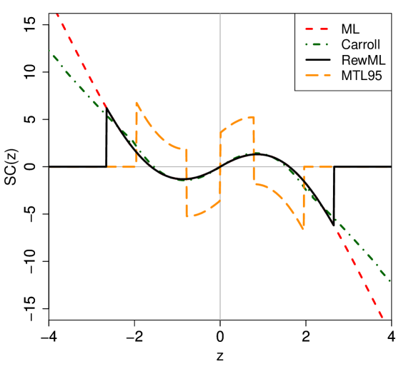
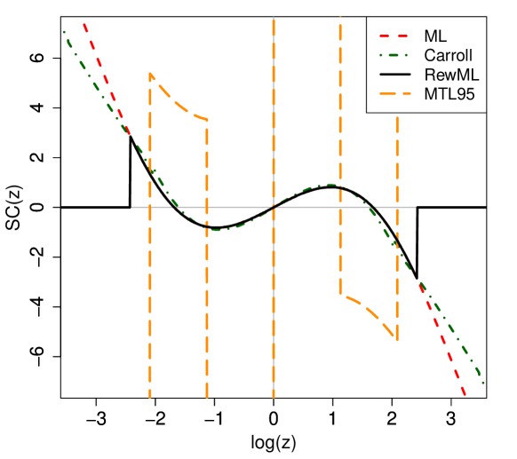
Figure 5: Sensitivity curves of estimators of the parameter $\lambda$ in the Yeo-Johnson (top) and Box-Cox (bottom) transformations, with sample size $n=100$.

The lower panel of Figure 5 shows the sensitivity curves for the Box-Cox transformation when the true parameter is $\lambda=0$, i.e. the clean data follows a lognormal distribution $F$. We now put $\log(z)$ on the horizontal axis, since this makes the plot more comparable to that for Yeo-Johnson in the top panel. Also here the ML and Carroll’s estimator have an unbounded sensitivity curve. Our RewML estimator has a redescending SC which again behaves similarly to the classical ML for small $|\log(z)|$, whereas the sensitivity to an extreme outlier is zero. The maximal trimmed likelihood estimator MTL95 has large jumps reaching values over 40 in the central region. Those peaks are not shown because the other curves would be hard to distinguish at that scale.

3 Simulation

3.1 Compared Methods

For the Box-Cox as well as the Yeo-Johnson transformations we perform a simulation study to compare the performance of several methods, including our proposal. The estimators under consideration are:

1. ML: the classical maximum likelihood estimator given by (11), or by (15) with all $w_{i}=1$.

2. Carroll: the robustified maximum likelihood estimator of [5] given by (17).

3. MTL: the maximum trimmed likelihood estimator of [18]. The notation MTL90 stands for the version with $h/n=90\%$ .

4. RewML: the proposed reweighted maximum likelihood estimator described in subsection 2.4.

5. RewMLnr: a variation on RewML in which the first step of subsection 2.4 applies (5) to the original Box-Cox or Yeo-Johnson transform instead of their rectified versions. This is not intended as a proposal, but included in order to show the advantage of rectification.

3.2 Data generation

We generate clean data sets as well as data with a fraction $\varepsilon$ of outliers. The clean data are produced by generating a sample of size $n$ from the standard normal distribution, after which the inverse of the BC or YJ transformation with a given $\lambda$ is applied. For contaminated data we replace a percentage $\varepsilon$ of the standard normal data by outliers at a fixed position before the inverse transformation is applied. For each such combination of $\lambda$ and $\varepsilon$ we generate $m=100$ data sets.

To be more precise, the percentage $\varepsilon$ of contaminated points takes on the values 0, 0.05, 0.1, and 0.15, where $\varepsilon=0$ corresponds to uncontaminated data. For the YJ transformation we take the true transformation parameter $\lambda$ equal to 0.5, 1.0, or 1.5 . We chose these values because for $\lambda$ between 0 and 2 the range of YJ given by (4) is the entire real line, so the inverse of YJ is defined for all real numbers. For the BC transformation we take $\lambda=0$ for which the range (3) is also the real line. For a given combination of $\varepsilon$ and $\lambda$ the steps of the data generation are:

1. Generate a sample $Y=(y_{1},\ldots,y_{n})$ from the standard normal distribution. Let $k>0$ be a positive parameter. Then replace a fraction $\varepsilon$ of the points in $Y$ by $k$ itself when $\lambda\leqslant 1$, and by $-k$ when $\lambda>1$.

2. Apply the inverse BC transformation to $Y$, yielding the data set $X$ given by$X=(g_{\lambda}^{-1}(y_{1}),\ldots,g_{\lambda}^{-1}(y_{n}))$. For YJ we put $X=(h_{\lambda}^{-1}(y_{1}),\ldots,h_{\lambda}^{-1}(y_{n}))$.

3. Estimate $\lambda$ from $X$ using the methods described in subsection 3.1.

The parameter $k$ characterizing the position of the contamination is an integer that we let range from 0 to 10.

We then estimate the bias and mean squared error (MSE) of each method by

bias $$:=\operatorname*{\mbox{ave}}_{j=1}^{n}{(\hat{\lambda}_{j}-\lambda)}$$

MSE $$:=\operatorname*{\mbox{ave}}_{j=1}^{n}{(\hat{\lambda}_{j}-\lambda)^{2}}$$

where $j=1,\ldots,m$ ranges over the generated data sets.

3.3 Results for the Yeo-Johnson transformation

We first consider the effect of an increasing percentage of contamination on the different estimators. In this setting we fix the position of the contamination by setting $k=10$. (The results for $k=6$ are qualitatively similar, as can be seen in section B of the supplementary material.) Figure 6 shows the bias and MSE of the estimators for an increasing contamination percentage $\varepsilon$ on the horizontal axis. The results in the top row are for data generated with $\lambda=0.5$, whereas the middle row was generated with $\lambda=1$ and the bottom row with $\lambda=1.5$ . In all rows the classical ML and the Carroll estimator have the largest bias and MSE, meaning they react strongly to far outliers, as suggested by their unbounded sensitivity curves in Figure 5. In contrast with this both RewML and RewMLnr perform much better as their bias and MSE are closer to zero. Up to about $5\%$ of outliers their curves are almost indistinguishable, but beyond that RewML outperforms RewMLnr by a widening margin. This indicates that using the rectified YJ transform in the first step of the estimator (see subsection 2.4) is more robust than using the plain YJ in that step, even though the goal of the entire 3-step procedure RewML is to estimate the $\lambda$ of the plain YJ transform.

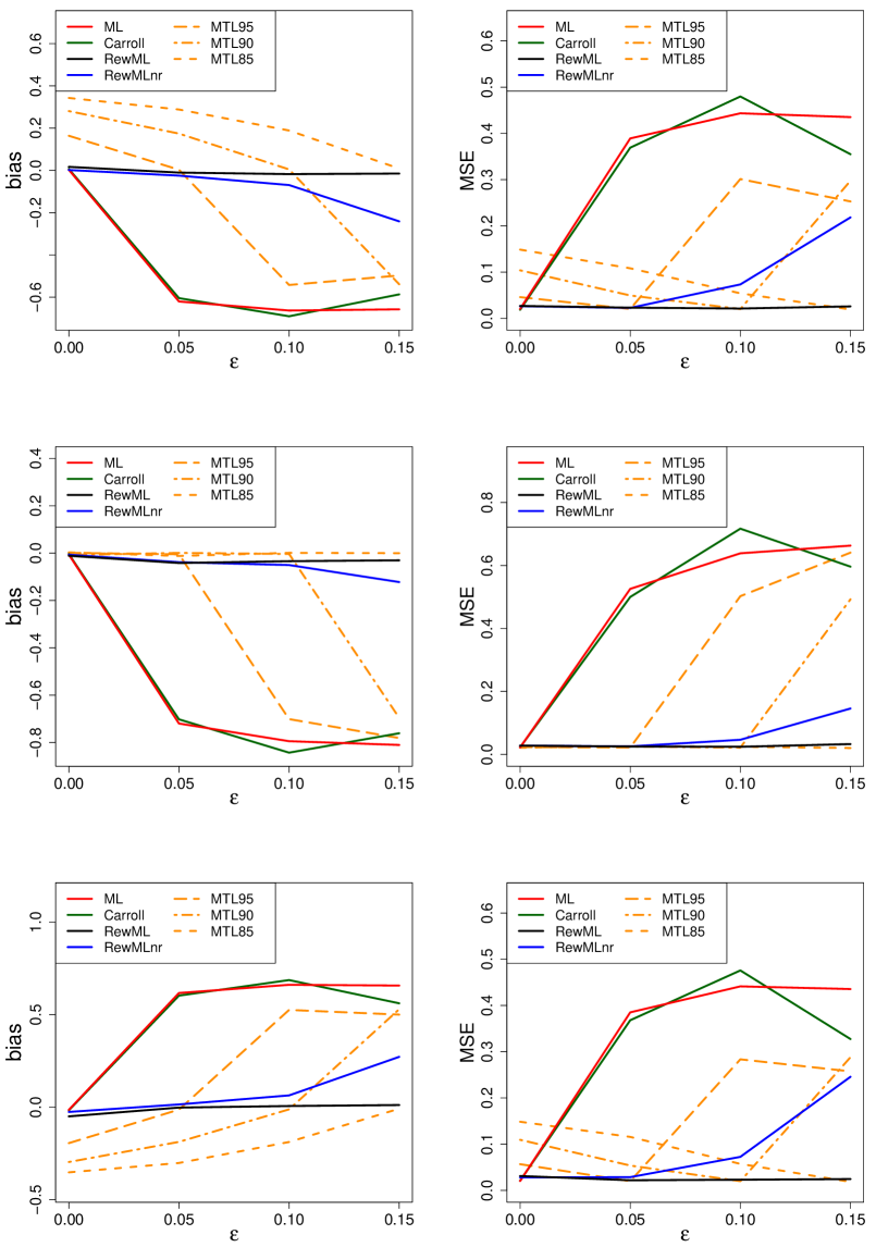
Figure 6: Bias (left) and MSE (right) of the estimated $\hat{\lambda}$ of the Yeo-Johnson transformation as a function of the percentage $\varepsilon$ of outliers, when the location of the outliers is determined by setting $k=10$. The true parameter $\lambda$ used to generate the data is 0.5 in the top row, 1.0 in the middle row, and 1.5 in the bottom row.

In the same Figure 6 we see the behavior of the maximum trimmed likelihood estimators MTL95, MTL90 and MTL85. In the middle row $\lambda$ is 1, and we see that MTL95, which fits $95\%$ of the data, performs well when there are up to $5\%$ of outliers and performs poorly when there are over $5\%$ of outliers. Analogously MTL90 performs well as long as there are at most $10\%$ of outliers, and so on. This is the intended behavior. But note that for $\lambda\neq 1$ these estimators also have a substantial bias when the fraction of outliers is below what they aim for, as can be seen in the top and bottom panels of Figure 6. For instance MTL85 is biased when $\varepsilon$ is under $15\%$, even for $\varepsilon=0\%$ when there are no outliers at all. So overall the MTL estimators only performed well when the percentage of trimming was equal to 1 minus the percentage of outliers in the data. Since the true percentage of outliers is almost never known in advance, it is not recommended to use the MTL method for variable transformation.

Let us now investigate what happens if we keep the percentage of outliers fixed, say at $\varepsilon=10\%$ , but vary the position of the contamination by letting $k=0,1,\ldots,10$. Figure 7 shows the resulting bias and MSE, with again $\lambda=0.5$ in the top row, $\lambda=1$ in the middle row, and $\lambda=1.5$ in the bottom row. For $k=0$ and $k=1$ the ML, Carroll, RewML and RewMLnr methods give similar results, since the contamination is close to the center so it cannot be considered outlying. But as $k$ increases the classical ML and the Carroll estimator become heavily affected by the outliers. On the other hand RewML and RewMLnr perform much better, and again RewML outperforms RewMLnr. Note that the bias of RewML moves toward zero when $k$ is large enough. We already noted this redescending behavior in its sensitivity curve in Figure 5.

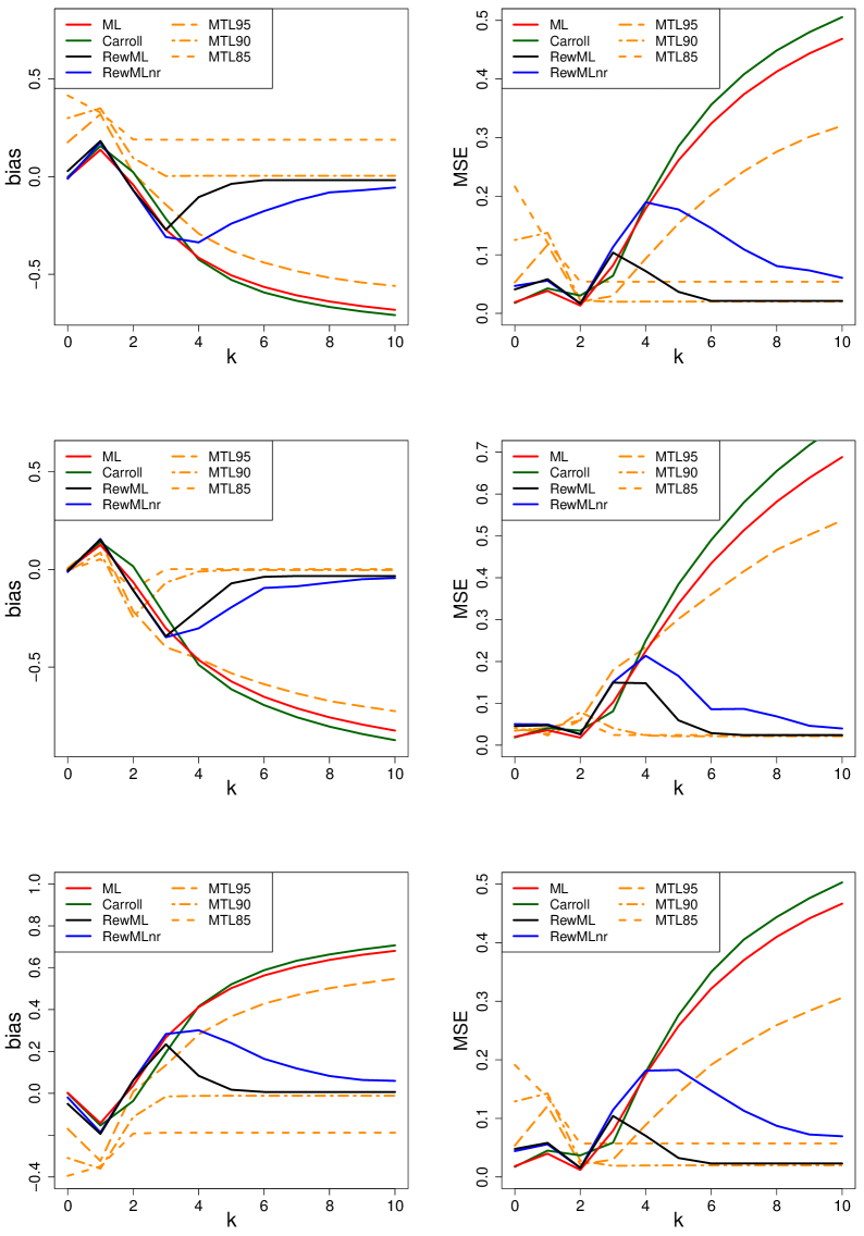
Figure 7: Bias (left) and MSE (right) of the estimated $\hat{\lambda}$ of the Yeo-Johnson transformation as a function of $k$ which determines how far the outliers are. Here the percentage of outliers is fixed at $10\%$ . The true parameter $\lambda$ used to generate the data is 0.5 in the top row, 1.0 in the middle row, and 1.5 in the bottom row.

The behavior of the maximum trimmed likelihood methods depends on the value of $\lambda$ used to generate the data. First focus on the middle row of Figure 7 where $\lambda=1$ so the clean data is generated from the standard normal distribution. In that situation both MTL90 and MTL85 behave well, whereas MTL95 can only withstand $5\%$ of outliers and not the $10\%$ generated here. One might expect the MTL method to work well as long as its $h$ excludes at least the number of outliers in the data. But in fact MTL85 does not behave so well when $\lambda$ differs from 1, as seen in the top and bottom panels of Figure 7, where the bias remains substantial even though the method expects 15% of outliers and there are only 10% of them. As in Figure 6 this suggests that one needs to know the actual percentage of outliers in the data in order to select the appropriate $h$ for the MTL method, but that percentage is typically unknown.

3.4 Results for the Box-Cox transformation

When simulating data to apply the Box-Cox transformation to, the most natural choice of $\lambda$ is zero since this is the only value for which the range of BC is the entire real line. Therefore we can carry out the inverse BC transformation on any data set generated from a normal distribution, so the clean data follows a log-normal distribution. The top panel of Figure 8 shows the bias and MSE for $10\%$ of outliers with $k=1,\ldots,10$. We see that the classical ML and the estimator of Carroll are sensitive to outliers when $k$ grows. Our reweighted method RewML performs much better. The RewMLnr method only differs from RewML in that it uses the non-rectified BC transform in the first step, and does not do as well since its bias goes back to zero at a slower rate.

The MTL estimators perform poorly here. The MTL95 version trims only $5\%$ of the data points so it cannot discard the 10% of outliers, leading to a behavior resembling that of the classical ML. But also MTL90 and MTL85, which trim enough data points, obtain a large bias which goes in the opposite direction, accompanied by a high MSE. The MSE of MTL90 and MTL85 lie entirely above the plot area.

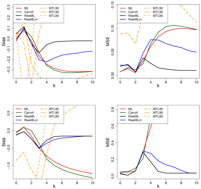
Figure 8: Bias (left) and MSE (right) of the estimated $\hat{\lambda}$ of the Box-Cox transformation as a function of $k$ which determines how far the outliers are. Here the percentage of outliers is fixed at $10\%$ . The true $\lambda$ used to generate the data is 0 in the top row and 1 in the bottom row.

Finally, we consider a scenario with $\lambda=1$. In that case the range of the Box-Cox transformation given by (3) is only $(-1,+\infty)$ so the transformed data cannot be normally distributed (which is already an issue for the justification of the classical maximum likelihood method). But the transformed data can have a truncated normal distribution. In this special setting we generated data from the normal distribution with mean 1 and standard deviation $1/3$, and then truncated it to $[0.01,1.99]$ (keeping $n=100$ points), so the clean data are strictly positive and have a symmetric distribution around 1. In the bottom panel of Figure 8 we see that the ML and Carroll estimators are not robust in this simulation setting. The trimmed likelihood estimators also fail to deliver reasonable results, with curves that often fall outside the plot area. On the other hand RewML still performs well, and again does better than RewMLnr.
The simulation results for a fixed outlier position at $k=6$ or $k=10$ with contamination levels $\varepsilon$ from 0% to 15% can be found in section B of the supplementary material, and are qualitatively similar to those for the YJ transform.

4 Empirical examples

4.1 Car data

Let us revisit the positive variable MPG from the TopGear data shown in the left panel of Figure 2. The majority of these data are already roughly normal, and three far outliers at the top deviate from this pattern. Before applying a Box-Cox transformation we first scale the variable so its median becomes 1. This makes the result invariant to the unit of measurement, whether it is miles per gallon or, say, kilometers per liter. The maximum likelihood estimator for Box-Cox tries to bring in the outliers and yields $\hat{\lambda}=-0.11$, which is close to $\lambda=0$ corresponding to a logarithmic transformation. The resulting transformed data in the left panel of Figure 9 are quite skewed in the central part, so not normal at all, which defeats the purpose of the transformation. This result is in sharp contrast with our reweighted maximum likelihood (RewML) method which estimates the transformation parameter as $\hat{\lambda}=0.84$. The resulting transformed data in the right panel does achieve central normality.

Figure 9: Normal QQ-plot of the Box-Cox transformed variable MPG using the ML estimate of $\lambda$ (left) and using the RewML estimate (right). The ML is strongly affected by the 3 outliers at the top, thereby transforming the central data away from normality. The RewML method achieves central normality and makes the outliers stand out more.

The variable Weight in the left panel of Figure 3 is not very normal in its center and has some outliers at the bottom. The classical ML estimate is $\hat{\lambda}=0.83$, close to $\lambda=1$ which would not transform the data at all, as we can see in the resulting left panel of Figure 10. In contrast, our RewML estimator obtains $\hat{\lambda}=0.09$ which substantially transforms the data, yielding the right panel of Figure 10. There the central part of the data is very close to normal, and the outliers at the bottom now stand out more, as they should.

Figure 10: Normal QQ-plot of the Box-Cox transformed variable Weight using the ML estimate of $\lambda$ (left) and using the RewML estimate (right). The ML masks the five outliers at the bottom, whereas RewML accentuates them and achieves central normality.

4.2 Glass data

For a multivariate example we turn to the glass data [11, 16] from chemometrics, which has become something of a benchmark. The data consists of $n=180$ archeological glass samples, which were analyzed by spectroscopy. Our variables are the intensities measured at 500 wavelengths. Many of these variables do not look normally distributed.

We first applied a Yeo-Johnson transformation to each variable with $\hat{\lambda}$ obtained from the nonrobust ML method of (11). For each variable we then standardized the transformed data $h_{\hat{\lambda}}(x_{i})$ to $(h_{\hat{\lambda}}(x_{i})-\hat{\mu}_{\mbox{\tiny{ML}},\hat{\lambda}})/\hat{\sigma}_{\mbox{\tiny{ML}},\hat{\lambda}}$ where $\hat{\mu}_{\mbox{\tiny{ML}},\hat{\lambda}}$ and $\hat{\sigma}_{\mbox{\tiny{ML}},\hat{\lambda}}$ are given by (12). This yields a standardized transformed data set with again 180 rows and 500 columns. In order to detect outliers in this matrix we compare each value to the interval $[-2.57,2.57]$ which has a probability of exactly $99\%$ for standard normal data. The top panel of Figure 11 is a heatmap of the standardized transformed data matrix where each value within $[-2.57,2.57]$ is shown as yellow, values above $2.57$ are red, and values below $-2.57$ are blue. This heatmap is predominantly yellow because the ML method tends to transform the data in a way that masks outliers, so not much structure is visible.

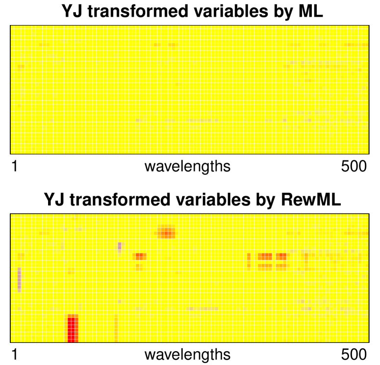
Figure 11: Heatmap of the glass data after transforming each variable (column) by a Yeo-Johnson transform with parameter $\lambda$ estimated by (top) the maximum likelihood method, and (bottom) the reweighted maximum likelihood method RewML. Yellow cells correspond to values in the central $99\%$ range of the normal distribution. Red cells indicate unusually high values, and blue cells have unusually low values.

Next, we transformed each variable by Yeo-Johnson with $\hat{\lambda}$ obtained by the robust RewML method. The transformed variables were standardized accordingly to $(h_{\hat{\lambda}}(x_{i})-\hat{\mu}_{\mbox{\tiny{W}},\hat{\lambda}})/\hat{\sigma}_{\mbox{\tiny{W}},\hat{\lambda}}$ where $\hat{\mu}_{\mbox{\tiny{W}},\hat{\lambda}}$ and $\hat{\sigma}_{\mbox{\tiny{W}},\hat{\lambda}}$ are given by (14) using the final weights in (13). The resulting heatmap is in the bottom panel of Figure 11. Here we see much more structure, with red regions corresponding to glass samples with unusually high spectral intensities at certain wavelengths. This is because the RewML method aims to make the central part of each variable as normal as possible, which allows outliers to deviate from that central region. The resulting heatmap has a subject-matter interpretation since wavelengths correspond to chemical elements. It indicates that some of the glass samples (with row numbers between 22 and 30) have a higher concentration of phosphor, whereas rows 57–63 and 74–76 had an unusually high amount of calcium. The red zones in the bottom part of the heatmap were caused by the fact that the measuring instrument was cleaned before recording the last 38 spectra.

4.3 DPOSS data

As a final example we consider data from the Digitized Palomar Sky Survey (DPOSS) described by [6]. We work with the dataset of 20000 stars available as dposs in the R package cellWise [14]. The data are measurements in three color bands, but for the purpose of illustration we restrict attention to the color band with the fewest missing values. Selecting the completely observed rows then yields a dataset of 11478 observations with 7 variables. Variables MAper, MTot and MCore measure light intensity, and variables Area, IR2, csf and Ellip are measurements of the size and shape of the images.

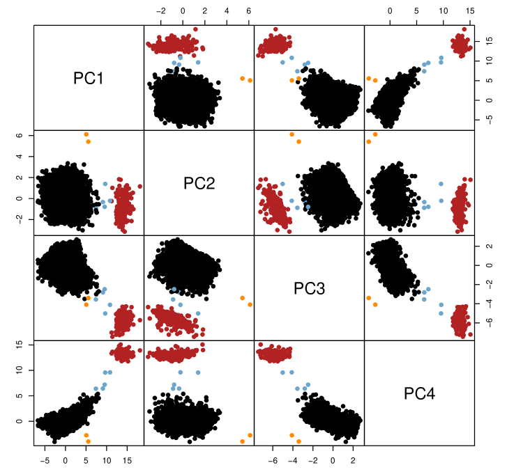
Figure 12: DPOSS data: pairs plot of the robust PCA scores after transforming the data with the robustly fitted YJ-transformation.

In order to analyze the data we first apply the YJ-transformation to each variable, with the $\hat{\lambda}$ estimates obtained from RewML. We then perform cellwise robust PCA [9]. We retained $k=4$ components, explaining 97% of the variance. Figure 12 is the pairs plot of the robust scores. We clearly see a large cluster of regular points with some outliers around it, and a smaller cluster of rather extreme outliers in red. The red points correspond to the stars with a high value of MAper. The blue points are somewhat in between the main cluster and the smaller cluster of extreme outliers. The two orange points are celestial objects with an extreme value of Ellip.

The left panel of Figure 13 contains the outlier map [10] of this robust PCA. Such an outlier map consists of two ingredients. The horizontal axis contains the score distance of each object $\bf{x}_{i}$. This is the robust Mahalanobis distance of the orthogonal projection of $\bf{x}_{i}$ on the subspace spanned by the $k$ principal components, and can be computed as

$$\mbox{SD}_{i}=\sqrt{\sum_{j=1}^{k}\frac{t_{ij}^{2}}{\lambda_{j}}}$$ (18)

where $t_{ij}$ are the PCA scores and $\lambda_{j}$ is the $j$-th largest eigenvalue. The vertical axis shows the orthogonal distance $\mbox{OD}_{i}$ of each point $\bf{x}_{i}$ , which is the distance between $\bf{x}_{i}$ and its projection on the $k$-dimensional subspace. We see that the red points form a large cluster with extreme $\mbox{SD}_{i}$ as well as $\mbox{OD}_{i}$. The blue points are intermediate, and the two orange points are still unusual but less extreme.

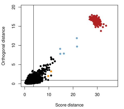
Figure 13: DPOSS data: outlier map of robust PCA applied to the YJ-transformed variables (left), and applied to the raw variables (right). The colors are those of Figure 12.

Interestingly, when applying robust PCA to the untransformed data we obtain the right panel of Figure 13 which shows a very different picture in which the red, blue and orange points are not clearly distinguished from the remainder. This outlier map appears to indicate a number of black points as most outlying, but in fact they should not be considered outlying since they are characterized by high values of Area and IR2 which are very right-skewed. When transforming these variables to central normality, as in the left panel, the values that appeared to be outlying become part of the regular tails of a symmetric distribution.

5 Discussion

In this discussion we address and clarify a few aspects of (robust) variable transformation.

Outliers in skewed data. The question of what is an outlier in a general skewed distribution is a rather difficult one. One could flag the values below a lower cutoff or above an upper cutoff, for instance given by quantiles of a distribution. But it is hard to robustly determine cutoffs for a general skewed dataset or distribution. Our viewpoint is this. If the data can be robustly transformed by BC or YJ towards a distribution that looks normal except in the tails, then it easy to obtain cutoffs for the transformed data, e.g. by taking their median plus or minus two median absolute deviations. And then, since the BC and YJ transforms are monotone, these cutoffs can be transformed back to the original skewed data or distribution. In this way we do not flag too many points. We have illustrated this for lognormal data in section C of the supplementary material.

How many outliers can we deal with? In addition to sensitivity curves, which characterize the effect of a single outlier, it is interesting to find out how many adversely placed outliers it takes to make the estimators fail badly. For RewML this turns out to be around 15% of the sample size, which is quite low compared to robust estimators of location or scale. But this is unavoidable, as asymmetry is tied to the tails of the distribution. Empirically, skewness does not manifest itself much in the central part of the distribution, say 20% of mass above and below the median. On each side we have 30% of mass left, and if the adversary is allowed to replace half of either portion (that is, 15% of the total mass) and move it anywhere, they can modify the skewness a great deal.

Prestandardization. In practice, one would typically apply some form of prestandardization to the data before trying to fit a transformation. For the YJ transformation, we can simply prestandardize the dataset $X=\{x_{1},\ldots,x_{n}\}$ by

$$\tilde{x}_{i}=\frac{x_{i}-\mbox{median}(X)}{\mbox{mad}(X)}$$ (19)

where mad is the median absolute deviation from the median. This is what we did in the glass and DPOSS examples. An advantage of this prestandardization is that the relevant $\lambda$ will typically be in the same range (say, from -4 to 6) for all variables in the data set, which is convenient for the computation of $\hat{\lambda}$. Before the BC transformation we cannot prestandardize by (19) since this would generate negative values. One option is to divide the original $x_{i}$ by their median so they remain positive and have median 1. But if the resulting data is tightly concentrated around 1, we may still require a huge positive or negative $\lambda$ to properly transform them by BC. Alternatively, we propose to prestandardize by

$$\tilde{x}_{i}=\exp\Big{(}\frac{\log(x_{i})-\mbox{median}(\log X)}{\mbox{mad}(\log X)}\Big{)}$$ (20)

which performs a standardization on the log scale and then transforms back to the positive scale. This again has the advantage that the range of $\lambda$ can be kept fixed when computing $\hat{\lambda}$ , making it as easy as applying the YJ transform after (19). A disadvantage is that the transformation parameter becomes harder to interpret, since e.g. a value of $\lambda=1$ no longer corresponds to a linear transformation, but $\lambda=0$ still corresponds to a logarithmic transform.

Tuning constants. The proposed method has some tuning parameters, namely the constant $c$ in (6), the cutoff $\Phi^{-1}(0.995)$ in the reweighting step, and the rectification points. The tuning of the constant $c$ is addressed in section A of the supplementary material. The second parameter is the constant $\Phi^{-1}(0.995)\approx 2.57$ in the weights (16). This weight function is commonly used in existing reweighting techniques in robust statistics. If the transformed data is normally distributed we flag approximately 1% of values with this cutoff, since $P(|Z|>\Phi^{-1}(0.995))=0.01$ if $Z\sim\mathcal{N}(0,1)$. Choosing a higher cutoff results in a higher efficiency, but at the cost of lower robustness. Generally, the estimates do not depend too much on the choice of this cutoff as long as it is in a reasonably high range, say from $\Phi^{-1}(0.975)$ to $\Phi^{-1}(0.995)$. A final choice in the proposal are the “rectification points” $C_{\ell}$ and $C_{u}$ for which we take the first and third quartiles of the data. Note that the constraints $C_{\ell}<0<C_{u}$ for YJ and $C_{\ell}<1<C_{u}$ for BC in (7)–(10) are satisfied automatically when prestandardizing the data as described in the previous paragraph. It is worth noting that these data-dependent choices of $C_{\ell}$ and $C_{u}$ do not create abrupt changes in the transformed data when moving through the range of possible values for $\lambda$ because the rectified transformations are continuous in $\lambda$ by construction. For instance, passing from $\lambda<1$ to $\lambda>1$ does not cause a jump in the transformed data because $\lambda=1$ corresponds to a linear transformation that is inherently rectified on both sides.

Models with transformed variables. The ease or difficulty of interpreting a model in the transformed variables depends on the model under consideration. For nonparametric models it makes little difference. For parametric models the transformations can make the model harder to interpret in some cases and easier in others, for instance where there is a simple linear relation in the transformed variables instead of a model with higher-order terms in the original variables. Also, the notion of leverage point in linear regression is more easily interpretable with roughly normal regressors, as it is related to the (robust) Mahalanobis distance of a point in regressor space.

The effect of the sampling variability of $\lambda$ on the inference in the resulting model is also model dependent. We expect that it will typically lead to a somewhat higher variability in the estimation. However, as the BY and YJ transformations are continuous and differentiable in $\lambda$ and not very sensitive to small changes of $\lambda$, the increase in variability is likely small. Moreover, if we apply BC or YJ transformations to predictor variables used in CART or Random Forest, the predictions and feature importance metrics stay exactly the same because the BC and YJ transformations are monotone.

6 Conclusion

In our view, a transformation to normality should fit the central part of the data well, and not be determined by any outliers that may be present. This is why we aim for central normality, where the transformed data is close to normal (gaussian) with the possible exception of some outliers that can remain further out. Fitting such a transformation is not easy, because a point that appears to be outlying in the original data may not be outlying in the transformed data, and vice versa.

To address this problem we introduced a combination of three ideas: a highly robust objective function (5), the rectified Box-Cox and Yeo-Johnson transforms in subsection 2.2 which we use in our initial estimator only, and a reweighted maximum likelihood procedure for transformations. This combination turns out to be a powerful tool for this difficult problem.

Preprocessing real data by this tool paves the way for applying subsequent methods, such as anomaly detection and well-established model fitting and predictive techniques.

Software availability

The proposed method is available as the function transfo() in the R [13] package cellWise [14] on CRAN, which also includes the vignette transfo_examples that reproduces all the examples in this paper. It makes uses of the R-packages gridExtra [3], reshape2 [19], ggplot2 [20] and scales [21].

Acknowledgement. This work was supported by grant C16/15/068 of KU Leuven.

Supplementary Material

Appendix A Choice of the tuning constant c

The function $\rho_{\mbox{\small{bw}}}$ in (6) contains a tuning constant $c$ which we set at 0.5. This tuning constant quantifies a trade-off between variance and robustness. For smaller values of $c$ the central part of Tukey’s $\rho$-function becomes more narrow, making it less likely that clean observations fall into this central part. For larger values of $c$ the opposite happens. Ideally, we would like the outliers to fall outside of the central region, and as many of the inliers as possible inside the central region. In section 5 it was argued that robustly fitting a skewness-correcting transform like BC or YJ can handle at most about 15% of outliers. We have tuned $c$ such that with 15% of extreme contamination, approximately 90% of the clean data fall into the central region.

The computation goes as follows. Suppose we have a data set $x_{1},\ldots,x_{n}$ of size $n$ and assume w.l.o.g. that $x_{1}\leq x_{2}\leq\ldots\leq x_{n}$. Assume furthermore that a fraction $1-\varepsilon$ can be transformed to a gaussian distribution, but the remaining fraction $\varepsilon$ consists of extreme outliers: $x_{i}\approx\infty$ for $i=(1-\varepsilon)n+1,\ldots,n$. (The situation where $x_{i}\approx-\infty$ for $i=1,\ldots,\varepsilon n$ is analogous.) For the regular observations, the differences between the observed and expected quantiles in the objective function (5) are close to

$$\Delta_{i}=\Phi^{-1}\left(\frac{i-1/3}{(1-\varepsilon)n+1/3}\right)-\Phi^{-1}\left(\frac{i-1/3}{n+1/3}\right)$$

for $i=1,\ldots,(1-\varepsilon)n$. We can verify that $P(|\Delta|\leq 0.5)\approx 88\%$ when $n\geqslant 100$.

Appendix B Additional simulations

In this section we show some additional simulation results. The plots complement the figures shown in the main text by considering a different position of the outliers ($k=6$) for an increasing contamination level $\varepsilon$, and also the case of $k=10$ for the BC transformation. The results shown here are in line with the conclusions of the main text.

B.1 the BC transformation

Figure 14 shows the effect of an increasing level of contamination on the estimates of the BC-transformation parameter when the position of the contamination is fixed at $k=10$. The proposed RewML did well, as it has a very stable performance which is not affected much by the increasing level of contamination. The reweighted estimator starting from the initial estimator without rectification (RewMLnr) performs less well, especially when the percentage of contamination increases. Carroll’s method and the classical maximum likelihood estimator are more heavily affected by the outliers, and perform poorly. The trimmed likelihood estimators display a very erratic behavior and are unreliable in this setup.

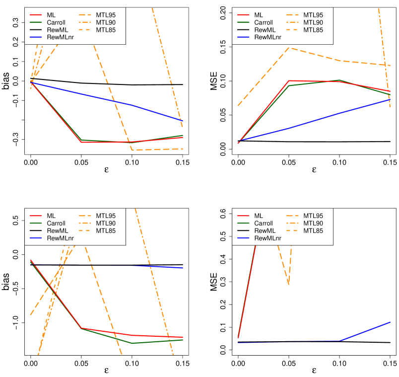
Figure 14: Bias (left) and MSE (right) of the estimated $\hat{\lambda}$ of the Box-Cox transformation as a function of the percentage $\varepsilon$ of outliers, when the location of the outliers is determined by setting $k=10$. The true parameter $\lambda$ used to generate the data is 0 in the top row 1 in the bottom row.

Figure 15 shows the effect of an increasing level of contamination on the estimates of the BC-transformation parameter when the position of the contamination is fixed at $k=6$. The general conclusions based from this figure are the same as for the case $k=10$ in the main text. We note that $k=6$ is slightly more difficult than $k=10$ in Figure 14, as evidenced by the more pronounced effect of increasing the contamination level.

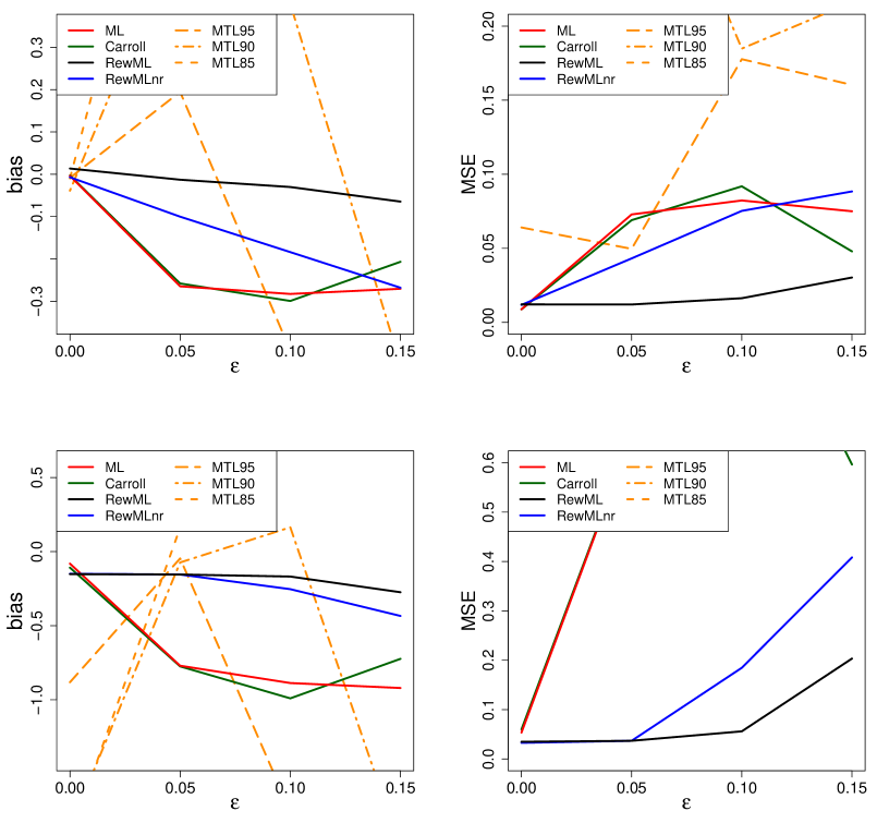
Figure 15: Bias (left) and MSE (right) of the estimated $\hat{\lambda}$ of the Box-Cox transformation as a function of the percentage $\varepsilon$ of outliers, when the location of the outliers is determined by setting $k=6$. The true parameter $\lambda$ used to generate the data is 0 in the top row, and 1 in the bottom row.

B.2 The YJ transformation

Figure 16 shows the effect of an increasing level of contamination on the estimates of the YJ transformation parameter when the position of the contamination is fixed at $k=6$. The performance of the estimators in this setting is very similar to the case of $k=10$, as can be seen in a comparison with Figure 6 of the main text. The trimmed estimators behave as they are supposed to for $\lambda=1$, but they become unreliable as soon as $\lambda$ deviates from 1. The ML estimator and Carroll’s estimator are more heavily influenced by the outliers, but the magnitude of the effect is slightly smaller than for $k=10$. The proposed RewML estimator performs best, and we again see that starting with an initial estimator without rectification (RewMLnr) substantially reduces the robustness of the reweighted estimator.

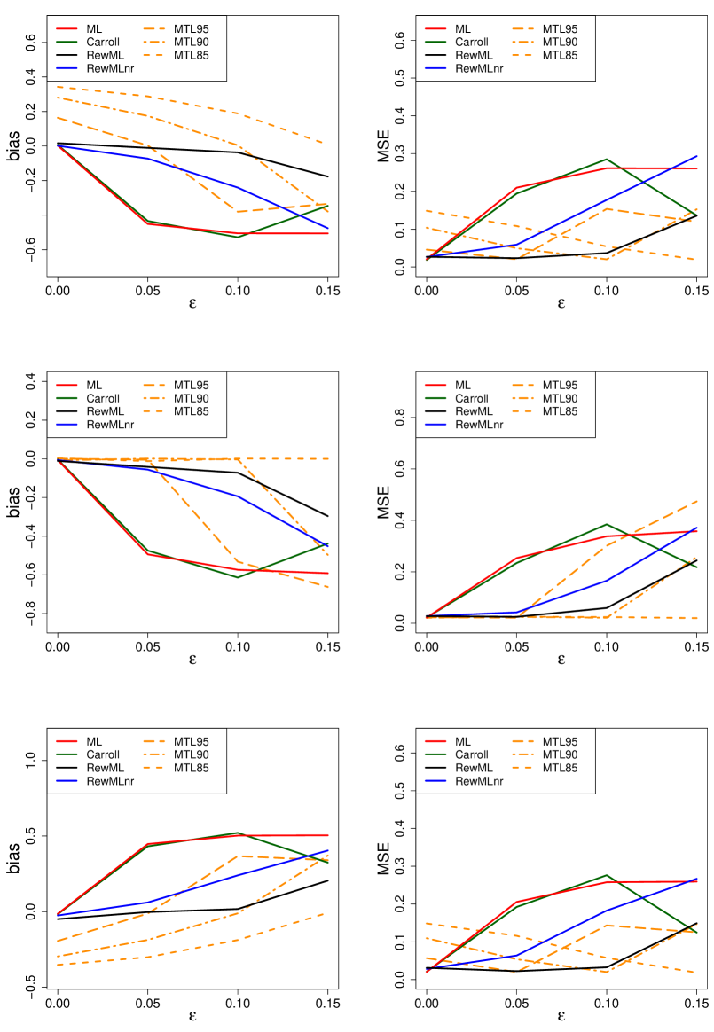
Figure 16: Bias (left) and MSE (right) of the estimated $\hat{\lambda}$ of the Yeo-Johnson transformation as a function of the percentage $\varepsilon$ of outliers, when the location of the outliers is determined by setting $k=6$. The true parameter $\lambda$ used to generate the data is 0.5 in the top row, 1.0 in the middle row, and 1.5 in the bottom row.

Appendix C False detections

We briefly investigate whether the proposed method is well-calibrated when it comes to outlier detection. More specifically, we track the number of “false positives”, i.e. the number of observations flagged as outliers when the data comes from a clean distribution. The clean data was generated from the lognormal distribution and the sample size was given by $n=10^{j}$ for $j=2,\ldots,6$. For each sample size 100 replications were run. These uncontaminated data were Box-Cox transformed with $\hat{\lambda}$ obtained from the proposed RewML estimator. Figure 17 shows boxplots of the percentage of points whose weight given by (16) is zero. As the sample size $n$ increases the fraction of flagged points approaches 1%, which is in line with the expected number of flagged points since the cutoffs on the transformed data in (16) are at the 0.005 and 0.995 quantiles.

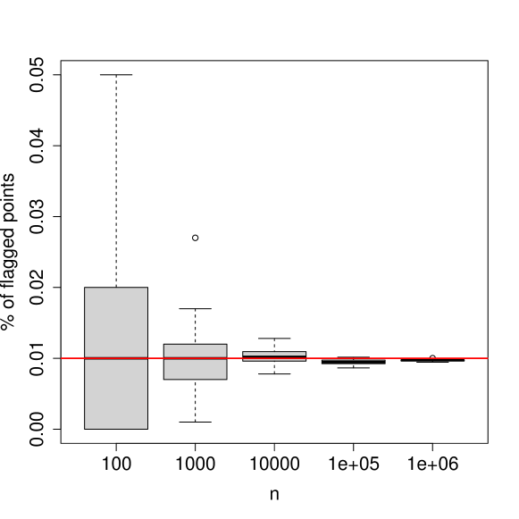
Figure 17: Percentage of points flagged as outlying in clean lognormal data, for various sample sizes. As the sample size increases, the fraction of flagged points approaches the expected frequency of 1%.

Appendix D Results with and without reweighting

In this section we illustrate the importance of the reweighting steps in RewML. Switching them off yields the initial estimator, which was left out of the figures in the main text because it fits a rectified transform, so it is effectively estimating a different transformation. Therefore, a direct comparison between the initial rectified estimator and the other estimators is questionable.

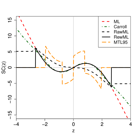
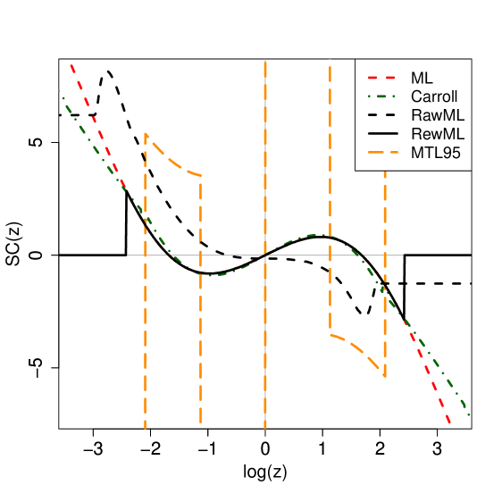
Figure 18: Sensitivity curves of estimators of the parameter $\lambda$ in the Yeo-Johnson (top) and Box-Cox (bottom) transformations, with sample size $n=100$.

Figure 18 shows the sensitivity curves including those of the initial estimator, denoted as RawML. We see that RawML has a bounded sensitivity curve, but it does not redescend to zero for large values of $|z|$. The sensitivity curve of the reweighted estimator behaves like the maximum likelihood estimator in the center, but is zero for large values of $|z|$. In the Box-Cox setting (lower panel of Figure 18) the sensitivity curve of RawML is asymmetric because the rectification is one-sided for $\lambda<1$, but the reweighting steps make the curve more symmetric again.

We now extend Figures 7 and 8 of the main text, which showed the bias and MSE of the estimators for 10% of contamination positioned at an increasing deviation $k$ from the center of the distribution. Figure 19 shows the results for the YJ transformation with the initial estimator added. We see that the initial estimator behaves roughly like the reweighted estimator for small $k$, but the bias does not redescend as the outliers are moved further away from the center. As a result, its MSE only stabilizes at a higher value of $k$.

Figure 20 shows the corresponding results for the BC transformation. A similar conclusion can be drawn here. For both the YJ and BC transforms it is clear that the application of the redescending weight function (16) reduces the effect of far outliers on $\hat{\lambda}$.

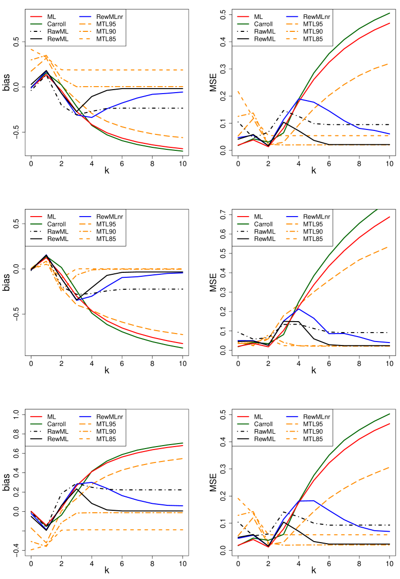
Figure 19: Bias (left) and MSE (right) of the estimated $\hat{\lambda}$ of the Yeo-Johnson transformation as a function of $k$ which determines how far the outliers are. Here the percentage of outliers is fixed at $10\%$ . The true parameter $\lambda$ used to generate the data is 0.5 in the top row, 1.0 in the middle row, and 1.5 in the bottom row.

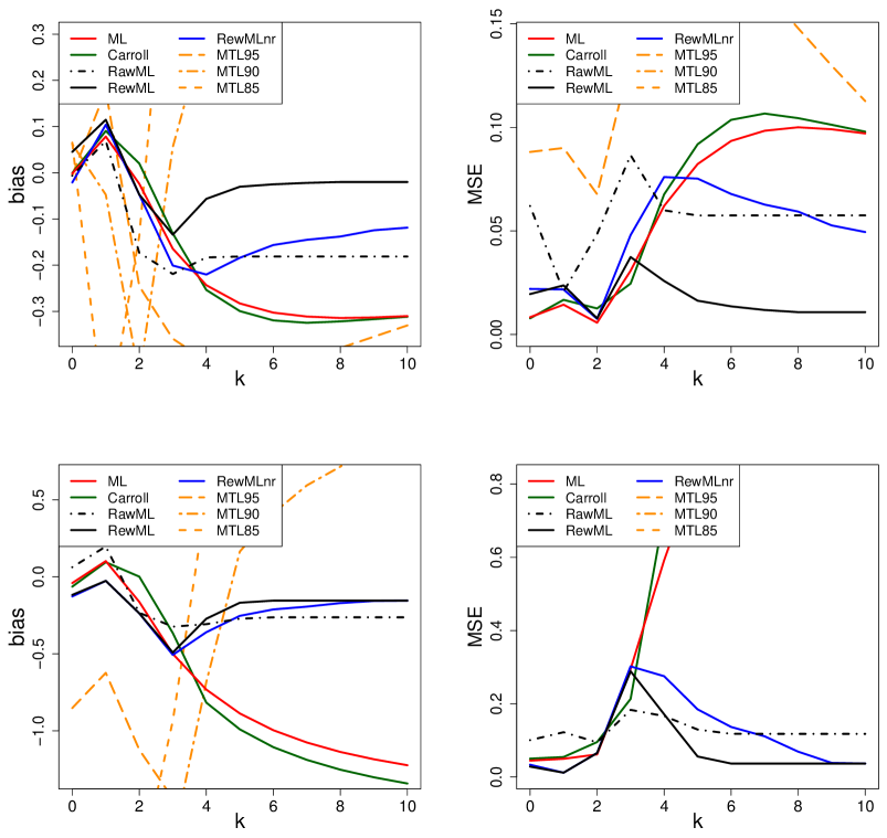
Figure 20: Bias (left) and MSE (right) of the estimated $\hat{\lambda}$ of the Box-Cox transformation as a function of $k$ which determines how far the outliers are. Here the percentage of outliers is fixed at $10\%$ . The true $\lambda$ used to generate the data is 0 in the top row and 1 in the bottom row.

References

- [1] Alfons, A.: robustHD: Robust Methods for High-Dimensional Data (2019). URL https://CRAN.R-project.org/package=robustHD. R package version 0.6.1
- [2] Andrews, D., Bickel, P., Hampel, F., Huber, P., Rogers, W., Tukey, J.: Robust Estimates of Location. Princeton University Press, Princeton, NJ (1972)
- [3] Auguie, B.: gridExtra: Miscellaneous Functions for ”Grid” Graphics (2017). URL https://CRAN.R-project.org/package=gridExtra. R package version 2.3
- [4] Box, G.E.P., Cox, D.R.: An analysis of transformations. Journal of the Royal Statistical Society. Series B 26, 211–252 (1964). URL http://www.jstor.org/stable/2984418
- [5] Carroll, R.J.: A robust method for testing transformations to achieve approximate normality. Journal of the Royal Statistical Society. Series B 42, 71–78 (1980). URL http://www.jstor.org/stable/2984740
- [6] Djorgovski, S., Gal, R., Odewahn, S., De Carvalho, R., Brunner, R., Longo, G., Scaramella, R.: The palomar digital sky survey (dposs). arXiv preprint astro-ph/9809187 (1998)
- [7] Hoaglin, D., Mosteller, F., Tukey, J.: Understanding Robust and Exploratory Data Analysis. Wiley, New York (1983)
- [8] Huber, P.: Robust Statistics. Wiley, New York (1981)
- [9] Hubert, M., Rousseeuw, P.J., Van den Bossche, W.: MacroPCA: An all-in-one PCA method allowing for missing values as well as cellwise and rowwise outliers. Technometrics 61, 459–473 (2019)
- [10] Hubert, M., Rousseeuw, P.J., Vanden Branden, K.: ROBPCA: A New Approach to Robust Principal Component Analysis. Technometrics 47, 64–79 (2005)
- [11] Lemberge, P., De Raedt, I., Janssens, K., Wei, F., Van Espen, P.: Quantitative z-analysis of 16th-17th century archaeological glass vessels using PLS regression of EPXMA and XRF data. Journal of Chemometrics 14, 751–763 (2000)
- [12] Marazzi, A., Villar, A.J., Yohai, V.J.: Robust response transformations based on optimal prediction. Journal of the American Statistical Association 104, 360–370 (2009)
- [13] R Core Team: R: A Language and Environment for Statistical Computing. R Foundation for Statistical Computing, Vienna, Austria (2020). URL https://www.R-project.org/
- [14] Raymaekers, J., Rousseeuw, P., Van den Bossche, W., Hubert, M.: cellWise: Analyzing Data with Cellwise Outliers (2020). URL https://CRAN.R-project.org/package=cellWise. R package version 2.2.2
- [15] Riani, M.: Robust transformations in univariate and multivariate time series. Econometric Reviews 28, 262–278 (2008)
- [16] Rousseeuw, P.J., Van den Bossche, W.: Detecting Deviating Data Cells. Technometrics 60, 135–145 (2018)
- [17] Tukey, J.W.: On the comparative anatomy of transformations. Annals of Mathematical Statistics 28, 602–632 (1957)
- [18] Van der Veeken, S.: Robust and nonparametric methods for skewed data. Ph.D. thesis, KU Leuven, Belgium (2010)
- [19] Wickham, H.: Reshaping data with the reshape package. Journal of Statistical Software 21(12), 1–20 (2007). URL http://www.jstatsoft.org/v21/i12/
- [20] Wickham, H.: ggplot2: Elegant Graphics for Data Analysis. Springer-Verlag New York (2016). URL https://ggplot2.tidyverse.org
- [21] Wickham, H., Seidel, D.: scales: Scale Functions for Visualization (2020). URL https://CRAN.R-project.org/package=scales. R package version 1.1.1
- [22] Yeo, I.K., Johnson, R.A.: A new family of power transformations to improve normality or symmetry. Biometrika 87, 954–959 (2000). URL http://www.jstor.org/stable/2673623