Abstract

Wigner distribution function of atomic system interacts locally with a deformed cavity is discussed. It is shown that, the deformed cavity has a destructive effect on the Wigner distribution function, where it decreases as one increases the deformation strength. The upper and lower bounds of the Wigner distribution function depends on the initial state settings of atomic system (entangled/product), the initial values of the dipole-dipole interaction’s and detuning parameters, and the external distribution weight and the phase angles. The possibility of suppressing the decay induced by the deformed cavity may be increased by increasing the dipole’s strength or the detuning parameter. We show that the distribution angles may be considered as a control external parameters, that maximize/ minimize the Wigner distribution function. This means that by controlling on the distribution angles, one can increase the possibility of suppressing the decoherence induced by the deformed cavity.

1 Introduction.

There are several studies have devoted to investigate the treatment of information between two users, who share different systems. Different studies have introduced to discuss many physical properties of atomic systems interact with a quantized cavity mode field [1]. Entanglement as a non-local property that generated between atoms inside different types of cavity modes is investigated for different systems[2]. The purity and the fidelity via deformed cavity field interacted with a pair of entangled qubits is discussed [3]. The information of the 2-qubit system is investigated within the magnetic field, non-Markovian environments, and acceleration [4, 5, 6]. On the other hand, the $q$-deformed of the Heisenberg algebra has many physical applications [7, 8, 9, 10, 11]. Lavagno[7] has obtained a generalized differential form of linear Schrödinger equation which involves the $q$-deformed Hamiltonian that is non-Hermitian. The geometry of the $q$-deformed phase space has investigated by Cerchiai, et. al [8]. Naderi et. al [9] have studied the temporal evolution of the atomic population inversion and quantum fluctuations of the two-photon $q$-deformed Jaynes-Cummings model. However, the framework of a one and two-photon $q$-deformed Dicke model by using a Bose-Einstein condensate is investigated in [10]. Meanwhile, the interaction between the deformed electromagnetic field and $N$-type four level atoms in the presence of a nonlinear Kerr medium is discussed[11].

As far as we know, the Wigner function play significant role in quantum distribution theory, where it indicates the quantumness analog by its negative values. Also, the Wigner function depicts the classicality by its positive values[12, 13]. For the atomic systems the Wigner function has not been studied widely. Among of these studies, for a two-qubit interacting with a quantized field system the Wigner distribution function is discussed analytically in the presence of pure phase noisy channel[14]. However, the Wigner function has been investigated the phase space for the quantum states based on finite fields with continuous or discrete degrees of freedom [15]. The time evolution of Wigner function in SU(2) algebra is analyzed for superconducting flux qubits [16]. Also, It has been reconstructed in SU(2) algebra for the accelerated three qubit system in the presence of some noisy channels [17].

In this manuscript, we are motivated to study the behavior of the Wigner distribution function of the atomic system consisted of two atoms. It is assumed that the atomic system either prepared in a maximum entangled or product state. This atomic system interacts locally with a cavity mode described ny imperfect (deformed) operators. We investigate the effect of the field and the atomic system’s parameters on the behavior of the Wigner distribution function. Moreover, the distribution angles are considered as an external parameter that can be used to maximize/ minimize the Wigner function distribution.

Therefore, the paper is organized this as : Sec. 2 is devoted to present the suggested physical model and demonstrate the exact solution of the evolution system. We review the mathematical form of the Wigner function in Sec.3. Finally, our results are summarized in Sec.4.

2 The suggest physical model.

Let us assume that the two users, Alice and Bob share an atomic system consists of 2-two level atoms (two-qubits), is prepared initially in a partial entangled state defined as,

$$|\psi_{ab}(0)\rangle = a_{1}|1,1\rangle+a_{2}|1,0\rangle+a_{3}|0,1\rangle+a_{4}|0,0\rangle.$$ (1)

where $|a_{1}^{2}+a_{2}^{2}+a_{3}^{2}+a_{4}^{2}=1$. The initial entanglement of this state depends on the choices of these coefficients. The two atoms may be prepared in an excited state if we set $a_{1}=1,a_{2}=0=a_{3}=a_{4}$. The maximum entangled state of Bell types can be obtained, if we set $a_{1}=a_{2}=\frac{1}{\sqrt{2}}$ and $a_{3}=a_{2}=0$. Otherwise, one can obtain a partial entangled/ separable state. It is assumed that, this atomic system interacts locally with a cavity deformed mode is initially prepared in the coherent state,

$$|\psi_{f}(0)\rangle = \sum_{n=0}{}q_{n}|n\rangle,\ q_{n}=\frac{\alpha^{n}}{\sqrt{n}}e^{\frac{-|\alpha|^{2}}{2}},$$ (2)

Therefore, initial state of the atomic-field system is given by,

$$\bigl{|}\psi_{s}(0)\bigr{\rangle}=\bigl{|}\psi_{ab}(0)\bigr{\rangle}\otimes\bigl{|}\psi_{f}(0)\bigr{\rangle}.$$ (3)

In the rotating-wave approximations, the Hamiltonian which describes the atomic-field system may be written as:

$$\hat{H}=\omega_{f}\hat{\mathcal{R}}^{\dagger}\hat{\mathcal{R}}+\sum_{i=1}^{2}\big{(}\Omega_{i}\hat{\sigma}_{z}^{(i)}+\lambda(\hat{\mathcal{R}}\hat{\sigma}_{+}^{(i)}+\hat{\mathcal{R}}^{\dagger}\hat{\sigma}_{-}^{(i)})\big{)}+i\kappa_{d}(\hat{\sigma}_{+}^{(1)}\hat{\sigma}_{-}^{(2)}-\hat{\sigma}_{-}^{(1)}\hat{\sigma}_{+}^{(2)}),$$ (4)

where $\omega_{f}$ and $\Omega_{i}$ are the frequencies of deformed field and the atomic system, respectively. The parameter $\lambda$ represents the coupling constant between the deformed field and the two atoms, while the parameter $g$ is the coupling constant between the two atoms. The operators $\hat{\sigma}_{z}^{(i)}$, $\hat{\sigma}_{+}^{(i)}$, and $\hat{\sigma}_{-}^{(i)}$ are the Pauli spin operators. Finally, the operators $\hat{\mathcal{R}}^{\dagger}$ and $\hat{\mathcal{R}}$ are the creation and annihilation operators of the generalized deformation field, which they are defined by well known bosonic operators $\hat{a}^{\dagger}$ and $\hat{a}$ as:

$$\hat{\mathcal{R}}^{\dagger}=\hat{a}^{\dagger}f(\hat{n}+1),\qquad\hat{\mathcal{R}}=\hat{a}f(\hat{n}),\quad\text{with}\quad\hat{n}=\hat{a}^{\dagger}\hat{a}.$$ (5)

These operators satisfy the commutation relation,

$$[\hat{\mathcal{R}},\hat{\mathcal{R}}^{\dagger}]=(\hat{n}+1)f^{2}(\hat{n}+1)+\hat{n}f^{2}(\hat{n}),\quad\text{with}\qquad[\hat{a},\hat{a}^{\dagger}]=I.$$ (6)

The function $f(n)$ is an arbitrary function represents the deformation function. In this contribution we consider the q-deformation [18], which is represented in terms of the $q$ parameter as,

$$f(n)=\sqrt{\frac{1-q^{n}}{n(1-q)}}.$$ (7)

In the Heisenberg picture, the equations of motion of the suggested system are given by means of the operators, $\hat{\mathcal{R}}$, $\hat{\mathcal{R}}^{\dagger}$ and $\hat{\sigma}_{z}^{(i)}$ as,

$$\frac{d\hat{\mathcal{R}}}{dt} = -i\omega_{f}\hat{\mathcal{R}}-i\lambda\sum_{i=1}^{2}\hat{\sigma}_{-}^{(i)},\qquad\frac{d\hat{\mathcal{R}}^{\dagger}}{dt}=i\omega_{f}\hat{\mathcal{R}}^{\dagger}+i\lambda\sum_{i=1}^{2}\hat{\sigma}_{+}^{(i)},$$

$$\frac{d\hat{\sigma}_{z}^{(1)}}{dt} = 2i\lambda(\hat{\mathcal{R}}\hat{\sigma}_{+}^{(1)}+\hat{\mathcal{R}}^{\dagger}\hat{\sigma}_{-}^{(1)})-2\kappa_{d}\sum_{i\neq j=1}^{2}\hat{\sigma}_{+}^{(i)}\hat{\sigma}_{-}^{(j)},$$

$$\frac{d\hat{\sigma}_{z}^{(2)}}{dt} = 2i\lambda(\hat{\mathcal{R}}\hat{\sigma}_{+}^{(2)}+\hat{\mathcal{R}}^{\dagger}\hat{\sigma}_{-}^{(2)})+2\kappa_{d}\sum_{i\neq j=1}^{2}\hat{\sigma}_{+}^{(i)}\hat{\sigma}_{-}^{(j)}.$$ (8)

The system of equations (2 may be used to describe the Hamiltonian model in eq.(4) in terms of constant of motion as:

$$\frac{\hat{H}}{\hbar}=\omega_{f}\hat{\mathcal{H}}_{0}+\hat{\mathcal{H}}_{I},\quad\text{where}\quad\hat{\mathcal{H}}_{0}=\hat{\mathcal{R}}^{\dagger}\hat{\mathcal{R}}+\frac{1}{2}\sum_{i=1}^{2}\hat{\sigma}_{z}^{(i)},$$ (9)

while the interaction Hamiltonian operator $\hat{\mathcal{H}}_{I}$ is;

$$\hat{\mathcal{H}}_{I}=\sum_{i=1}^{2}\big{(}\frac{\Delta_{i}}{2}\hat{\sigma}_{z}^{(i)}+\lambda(\hat{\mathcal{R}}\hat{\sigma}_{+}^{(i)}+\hat{\mathcal{R}}^{\dagger}\hat{\sigma}_{-}^{(i)})\big{)}+i\kappa_{d}(\hat{\sigma}_{+}^{(1)}\hat{\sigma}_{-}^{(2)}-\hat{\sigma}_{-}^{(1)}\hat{\sigma}_{+}^{(2)}),\quad$$ (10)

where the detuning parameter, $\Delta_{i}=2\Omega_{i}-\omega_{f},\quad i=1,2$. At any $t>0$ the time evaluation of the initial atomic-field system (3) may be written as,

$$|\psi_{s}(t)\rangle=\sum_{n=0}^{\infty}(C^{n}_{1}(t)|1,1,n\rangle+C_{2}^{n}(t)|1,0,n+1\rangle+C^{n}_{3}(t)|0,1,n+1\rangle+C^{n}_{4}(t)|0,0,n+2\rangle),$$ (11)

where $C_{i},i=1,..4$, with $\sum_{j=1}^{4}|C_{j}|^{2}=1$ are the solutions of the following system of differential equations,

$$\begin{bmatrix}\partial_{t}C^{n}_{1}(t)\\ \partial_{t}C^{n}_{2}(t)\\ \partial_{t}C^{n}_{3}(t)\\ \partial_{t}C^{n}_{4}(t)\end{bmatrix}=-i\begin{bmatrix}0&\nu_{1}(n)&\nu_{1}(n)&0\\ \nu_{1}(n)&\delta&i\kappa_{d}&\nu_{2}(n)\\ \nu_{1}(n)&-\delta&-i\kappa_{d}&\nu_{2}(n)\\ 0&\nu_{2}(n)&\nu_{2}(n)&0\end{bmatrix}\begin{bmatrix}C^{n}_{1}(t)\\ C^{n}_{2}(t)\\ C^{n}_{3}(t)\\ C^{n}_{4}(t)\end{bmatrix}$$ (12)

where $\nu_{1}(n)=\lambda f(n+1)\sqrt{n+1}$, $\nu_{2}(n)=\lambda f(n+2)\sqrt{n+2}$, and $\Delta_{1}-\Delta_{2}=2\delta$, where we simulating that the atomic system in an exact resonance case, i.e. $\Delta_{1}+\Delta_{2}=0$. The solution of this system is obtained analytically as,

$$C^{n}_{1}(t) = q_{n}a_{1}-\frac{K_{1}}{\mu^{2}}(1-\cos\mu t)-\frac{i\nu_{1}(n)q_{n+1}(a_{2}+a_{3})}{\mu}\sin\mu t,$$

$$C^{n}_{2}(t) = q_{n+1}a_{2}\cos\mu t-\frac{\chi}{\mu^{2}}(1-\cos\mu t)-\frac{iG_{1}}{\mu}\sin\mu t,$$

$$C^{n}_{3}(t) = q_{n+1}a_{3}\cos\mu t+\frac{\chi}{\mu^{2}}(1-\cos\mu t)-\frac{iG_{2}}{\mu}\sin\mu t,$$

$$C^{n}_{4}(t) = q_{n+2}a_{4}-\frac{K_{2}}{\mu^{2}}(1-\cos\mu t)-\frac{i\nu_{2}(n)q_{n+1}(a_{2}+a_{3})}{\mu}\sin\mu t,$$ (13)

with

$$K_{j} = \nu_{j}(n)q_{n+1}(a_{2}-a_{3})(\delta-i\kappa_{d})+2\nu_{j}(n)(q_{n}a_{1}\nu_{1}(n)+q_{n+1}a_{2}\nu_{2}(n)),\quad j=1,2$$

$$\chi = (q_{n}a_{1}\nu_{1}(n)+q_{n+2}a_{4}\nu_{2}(n))(\delta-i\kappa_{d})-q_{n+1}(a_{2}-a_{3})(\nu_{1}^{2}(n)+\nu_{1}^{2}(n)),$$

$$G_{1} = q_{n}a_{1}\nu_{1}(n)+q_{n+1}a_{2}\delta+iq_{n+1}a_{3}\kappa_{d}+q_{n+2}a_{4},$$

$$G_{2} = q_{n}a_{1}\nu_{1}(n)-iq_{n+1}a_{2}\kappa_{d}-q_{n+1}a_{3}\delta+q_{n+2}a_{4},$$ (14)

where $\mu=\sqrt{\delta^{2}+2(\nu_{1}^{2}(n)+\nu_{1}^{2}(n))+\kappa_{d}^{2}}$. Now, by using Eqs.(11 and (2) , the final state of the total systems can be written as,

$$\begin{split}\hat{\rho_{s}}=|\psi_{s}(t)\rangle\langle\psi_{s}(t)|.\end{split}$$ (15)

The main task of this manuscript is investigating the effect of the deformed field on the behavior of the Wigner distribution function. Therefore, it is important to obtain the states of Alice-Bob atomic subsystems and the Alice subsystem. to obtain the atomic state, one traces out the field degree of freedom, i.e. $\hat{\rho}_{A,B}=Tr_{field}|\psi(t)\rangle\langle\psi(t)|$. So, the reduced density operator of Alice, and Bob atomic subsystem is given by,

$$\begin{split}\hat{\rho}_{A,B}&=\begin{bmatrix}|C^{n}_{1}(t)|^{2}&C^{n+1}_{1}(t)C^{n^{*}}_{2}(t)&C^{n+1}_{1}(t)C^{n^{*}}_{3}(t)&C^{n+2}_{1}(t)C^{n^{*}}_{4}(t)\\ C^{n+1^{*}}_{1}(t)C^{n}_{2}(t)&|C^{n1}_{2}(t)|^{2}&C^{n}_{2}(t)C^{n^{*}}_{3}(t)&C^{n+1}_{2}(t)C^{n^{*}}_{4}(t)\\ C^{n+1^{*}}_{1}(t)C^{n}_{3}(t)&C^{n^{*}}_{2}(t)C^{n}_{3}(t)&|C^{n}_{3}(t)|^{2}&C^{n+1}_{3}(t)C^{n^{*}}_{4}(t)\\ C^{n+2^{*}}_{1}(t)C^{n}_{4}(t)&C^{n+2^{*}}_{1}(t)C^{n}_{4}(t)&C^{n+1^{*}}_{3}(t)C^{n}_{4}(t)&|C^{n}_{4}(t)|^{2}\end{bmatrix}\end{split}$$ (16)

On the other hand, one can obtain the reduced density operator of Alice atomic subsystem as,

$$\hat{\rho}_{A} = Tr_{B}[\hat{\rho}_{A,B}]$$ (17)

$$= \big{(}|C^{n}_{1}(t)|^{2}+|C^{n}_{2}(t)|^{2}\big{)}|1\rangle_{A}\langle 1|+\big{(}|C^{n}_{3}(t)|^{2}+|C^{n}_{4}(t)|^{2}\big{)}|0\rangle_{A}\langle 0|$$

$$+ \bigg{(}C^{n+1}_{1}(t)C^{n^{*}}_{3}(t)+C^{n+1}_{2}1(t)C^{n^{*}}_{4}(t)\bigg{)}|1\rangle_{A}\langle 0|+h.c.$$

3 Wigner Distribution Function.

The atomic Wigner probability distribution in SU(2) algebra is reconstructed in the angular momentum basis of a two-level atom $|m,\frac{1}{2}\rangle,m=-\frac{1}{2},\frac{1}{2}$ as follows [19, 6]:

$$\mathcal{W}_{\hat{\rho}}(\theta,\phi)=Tr[\hat{\rho}_{a,b}\hat{A}_{a}(\theta,\phi)\hat{A}_{b}(\theta,\phi)],$$ (18)

where the operator $\hat{A}_{i}(\theta,\phi)$, $i=a,b$ corresponds to the two subsystem Alice and Bob is defined by:

$$\hat{A}_{i}(\theta,\phi)=\sqrt{2\pi}\sum_{L_{i}=0}^{1}\sum_{M=-L}^{L}\hat{T}^{(i)^{\dagger}}_{L,M}Y^{i}_{L,M}(\theta,\phi),$$ (19)

The $Y^{i}_{L,M}(\theta,\phi)$ are the spherical harmonics functions, while $T^{(i)^{\dagger}}_{L,M}=(-1)^{M}T_{L,-M}$ are the orthogonal irreducible tensor operators which are represented in Hilbert space as a linear combination by [20]:

$$\hat{T}^{(i)^{\dagger}}_{L,M}=(-1)^{M}\sqrt{\frac{2L+1}{2}}\sum_{m,m^{\prime}=-\frac{1}{2}}^{\frac{1}{2}}C^{\frac{1}{2},m^{\prime}}_{\frac{1}{2},m;L,-M}|\frac{1}{2},m^{\prime}\rangle\langle\frac{1}{2},m|.$$ (20)

The coefficient $C^{\frac{1}{2},m^{\prime}}_{\frac{1}{2},m;L,-M}$ is the Clebsch-Gordan coupling coefficient, where $0\leq L_{i}\leq 1$, and $-L\leq M\leq L$. Then, the Wigner probability distribution is given by,

$$\begin{split}\mathcal{W}_{\hat{\rho}}(\theta,\phi)=2\pi\ Tr&\bigg{[}\hat{\rho}_{AB}\prod_{i}^{n}\big{(}\hat{T}^{i^{\dagger}}_{0,0}Y^{i}_{0,0}(\theta,\phi)+\sum_{n=-1}^{1}\hat{T}^{i^{\dagger}}_{1,n}Y^{i}_{1,n}(\theta,\phi)\big{)}\bigg{]},\end{split}$$ (21)

where,

$$\begin{split}&\hat{T}^{(i)^{\dagger}}_{0,0}=\frac{1}{\sqrt{2}}(|0\rangle_{i}\langle 0|+|1\rangle_{i}\langle 1|),\quad\hat{T}^{(i)^{\dagger}}_{1,0}=\frac{-1}{\sqrt{2}}(|0\rangle_{i}\langle 0|-|1\rangle_{i}\langle 1|),\quad\hat{T}^{(i)^{\dagger}}_{1,-1}=|1\rangle_{i}\langle 0|\quad\\ &\hat{T}^{(i)^{\dagger}}_{1,1}=-|0\rangle_{i}\langle 1|,\quad|1\rangle=|\frac{1}{2},\frac{1}{2}\rangle,\quad|0\rangle=|\frac{1}{2},\frac{-1}{2}\rangle.\end{split}$$

After some straightforward calculation, one can obtain the Wigner distribution function of Alice-Bob subsystem as,

$$\begin{split}\mathcal{W}_{\hat{\rho}}(\theta,\phi)&=2\pi\bigg{[}|C^{n}_{1}(t)|^{2}\varLambda^{2}_{11}+\big{(}|C^{n}_{2}(t)|^{2}+|C^{n}_{3}(t)|^{2}\big{)}\varLambda_{11}\varLambda_{00}+|C^{n}_{4}(t)|^{2}\varLambda^{2}_{00}+\\ &+\bigg{(}(C^{n^{*}}_{2}(t)+C^{n^{*}}_{3}(t))C^{n+1}_{1}(t)\varLambda_{11}\varLambda_{01}+C^{n}_{2}(t)C^{n^{*}}_{3}(t)\varLambda_{01}\varLambda_{10}+\\ &+(C^{n+1}_{3}(t)+C^{n+1}_{2}(t)(t))C^{n^{*}}_{4}(t)\varLambda_{00}\varLambda_{01}+C^{n+2^{*}}_{1}(t)C^{n^{*}}_{4}(t)\varLambda^{2}_{01}+h.c.\bigg{)}\bigg{]}\end{split}$$ (22)

where the functions $\varLambda_{ij}$ are defined by the following spherical harmonics,

$$\begin{split}&\varLambda_{11}=\frac{1}{\sqrt{2}}(Y_{0,0}(\theta,\phi)-Y_{1,0}(\theta,\phi)),\quad\varLambda_{01}=-Y_{1,1}(\theta,\phi),\\ &\varLambda_{10}=Y_{1,-1}(\theta,\phi),\quad\varLambda_{00}=\frac{1}{\sqrt{2}}(Y_{0,0}(\theta,\phi)+Y_{1,0}(\theta,\phi)).\end{split}$$

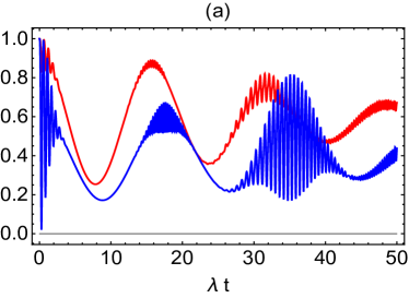
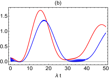
Figure 1: Wigner distribution function against the scaled time $\lambda t$, where there is no deformation, i.e., $f(n)=1$. where $\theta=\pi/2$, $\phi=\pi$ and $\delta=1$, $\kappa_{d}=1,5$ for red and blue curve, respectively. (a) The atomic system is initially prepared in a maximum entangled state $\bigl{|}\psi_{2}\bigr{\rangle}=\frac{1}{\sqrt{2}}(\bigl{|}11\bigr{\rangle}+\bigl{|}00\bigr{\rangle})$. (b) The atomic system is initially prepared in a product state $\bigl{|}\psi_{1}\bigr{\rangle}=\frac{1}{2}(\bigl{|}0\bigr{\rangle}+\bigl{|}1\bigr{\rangle})_{A}(\bigl{|}0\bigr{\rangle}+\bigl{\langle}1\bigr{|})_{B}$.

In Fig.(1), we show the behavior of the Wigner distribution function in the presences of perfect cavity operator, namely $f(n)=1$, where we consider that the atomic system either prepared in a maximum entangled state of Bell type (Fig.1 a) or in a product state (Fig. 1b). As it is displayed from Fig.(1), the Wigner distribution function oscillates between its lower and upper bounds. The maximum and minimum bounds depend on the strength of the dipole-dipole interaction, $\kappa_{d}$. The behavior of $\mathcal{W}_{p}$. The phenomena of the collapse and revival behavior of the Wigner distribution function is depicted clearly in Fig.(1.a), where the atomic system is initially prepared in the maximum entangled state. On the other hand, the maximum values of the Wigner distribution function that depicted in Fig.(1.b), where the atomic system is initially prepared in a product state is much larger than that displayed in Fig.(1.a).

Our main task is investigating the behavior of $\mathcal{W}_{p}$, when the atomic system interacts with a deformed cavity, which means that the criterion annihilation operators are imperfect (deformed). In this context, we discuss the effect of the initial state settings of the atomic system, the initial strength of the dipole-dipole interaction, the deformation strength, and the distribution angles, on the behavior of the Wigner distribution function.

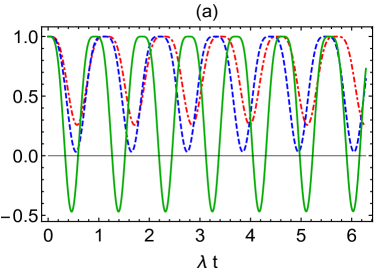
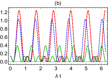
Figure 2: Wigner distribution function against the scaled time $\lambda t$, where there is no deformation, i.e.,$f(n)=\sqrt{\frac{1-q^{n}}{n(1-q)}}.$. $\phi=\pi,\theta=\pi/2,\delta=1,\kappa_{d}=5,q=0.1(red-dotdash),0.4(blue-dash),0.8(green-solid)$. (a) The atomic system is initially prepared in a maximum entangled state $\bigl{|}\psi_{2}\bigr{\rangle}=\frac{1}{\sqrt{2}}(\bigl{|}11\bigr{\rangle}+\bigl{|}00\bigr{\rangle})$. (b) The atomic system is initially prepared in a product state $\bigl{|}\psi_{1}\bigr{\rangle}=\frac{1}{2}(\bigl{|}0\bigr{\rangle}+\bigl{|}1\bigr{\rangle})_{A}(\bigl{|}0\bigr{\rangle}+\bigl{\langle}1\bigr{|})_{B}$ .

In Fig.(2), we discuss the effect of the deformed field operator on the behavior of the Wigner distribution function $\mathcal{W}_{p}$, where we assume that the atomic system is either prepared in a maximum entangled or product state. As it is displayed in Fig.(2.a), where the system is initially prepared in a maximum entangled state of Bell type, the Wigner distribution function is maximum as $\lambda t=0$ and decreases as soon as the interaction between the atomic and the field systems is switched on. The decreasing decay depends on the strength of the deformation, where at small values of $q=0.1$ the lower bound is larger than that depicted at large values. The behavior of the distribution Wigner function is repeated periodically at further values of the interaction. In Fig.(2.b), it is assumed that the atomic system is prepared in a product state. Similarly the periodic behavior is displayed, where $\mathcal{W}_{p}$ fluctuated between its lower and maximum bounds. However, the maximum values of the Wigner distribution is shown at small values of the deformation strength.

From Fig.(2), it is clear that the large deformation strength decreases the Wigner function distributing the displayed for atomic system is initially prepared in a maximum entangled state. On the other hand, it suppress the expected increases behavior of the Wigner function distribution, where the smallest upper values of $\mathcal{W}_{p}$ are displayed at large values of deformation strength.

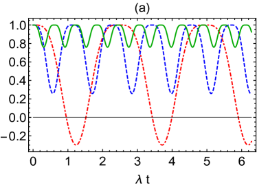
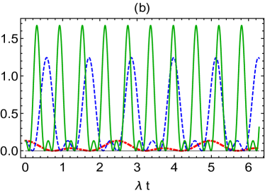
Figure 3: The same as Fig. (2) with $\phi=\pi,\theta=\pi/2,\delta=1,q=0.1,\kappa_{d}$= 1(red-dot dash),5(blue-dash),10(green-solid).

In Fig.(3), we investigate the effect of the dipole-dipole interaction strength on the behavior of the Wigner distribution function in the presences of deformed field cavity. The behavior is similar to that displayed in Fig.(1), namely $\mathcal{W}_{p}$ oscillates periodically between its lower and upper bounds. However, the number of oscillations and their amplitudes depends on the dipole-dipole interaction strength, $\kappa_{d}$. It is clear that, at $\lambda t=0$ the Wigner Distribution function for a system is initially prepared in a MES is maximum. However as the interaction is switched on, $\mathcal{W}_{p}$ decreases gradually to reach their minimum values. The decay on the Wigner distribution can be countered by increasing the strength of the dipole-dipole interaction, where as it is displayed from Fig.(3), as on increase $\kappa_{d}$, the amplitudes of the oscillations are small, which means that the decay is small. However, as on decreases $\kappa_{d}$, the deformed cavity has a stronger effect and consequently the decay rate is large.

Fig.(3.b) describes the behavior of Wigner Distribution $\mathcal{W}_{p}$, where it is assumed that the atomic system is initially prepared in a product state. It is clear that $\mathcal{W}_{p}$ oscillates periodically, where their amplitudes increase as one increases the dipole strength, $\kappa_{d}$. This means that the destructive effect of the deformed cavity may be Withstand by increasing the strength of the dipole strength. On the other hand, at small values of the interaction strength $\kappa_{d}$, the Wigner distribution is very weak against the deformed cavity, where their amplitudes are very small and vanish periodically.

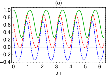
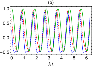
Figure 4: Wigner distribution function against the scaled time $\lambda t$, for atomic system is initially prepared in a maximum entangled state $\bigl{|}\psi_{2}\bigr{\rangle}=\frac{1}{\sqrt{2}}(\bigl{|}11\bigr{\rangle}+\bigl{|}00\bigr{\rangle})$ where we set $\theta=\pi/4,\delta=1,g=5,\phi=\pi/4(red-dotdash),\pi/2(blue-dash),\pi(green-solid)$ (a)$q=0.1(b)q=0.8$

In Fig.(4), we discuss the effect of the distribution angles $\theta$ and $\phi$ on the behavior of the deformed Wigner Function $\mathcal{W}_{p}$, where we set the weight angle $\theta=\pi/4$ and different values of the phase angle $\phi$. The general behavior shows that $\mathcal{W}_{p}$ oscillates periodically between its maximum and minimum values. It is clear that, these parameters play as control parameter on maximize/ minimize the Wigner distribution function. As it is clear from Fig.(4) the amplitudes of $\mathcal{W}_{p}$ increases as the deformation strength increases, and consequently the upper bounds are improved. However, different choices of the phase angle maximize the amplitudes of the Wigner distribution. On the other hand, as it is depicted from Fig.(3a) and (4), the weight angle $\theta$ has a clear effect on increasing the amplitudes’ oscillations, hence the minimum values decreases. This means that by controlling on the distribution angles, one can increase the possibility of suppressing the decoherence induced by the deformed cavity.

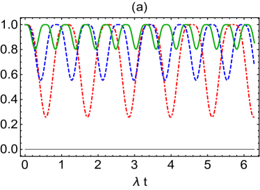
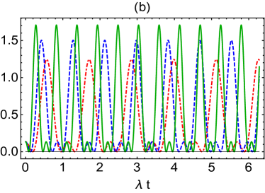
Figure 5: The same as Fig. (2) with $\phi=\pi,\theta=\pi/2,q=0.1,g=5,\delta=$1(red-dot dash),5(blue-dash), 10(green-solid).

In Fig.(5), we investigate the effect of the detuning parameter on the behavior of the deformed Wigner function for a system is initially prepared in a maximum entangled or product state. It is important to mention that the detuning $\delta=\Delta_{1}-\Delta_{2}$, where $\Delta_{i},i=a,b$ is the frequency of each atom, namely the larger $\delta$ the smaller atomic frequency. A similar behavior of, $\mathcal{W}_{p}$ is displayed, where it oscillates between its maximum and lower bounds. As it is clear from Fig.(5.a), at small values of $\delta$, the decreasing rate of the Wigner function is large. However, the oscillations’s amplitudes decreases as $\delta$ increases and consequently the lower bounds of the Wigner function are improved. The similar effect is predicted in Fig.(5.b), where the atomic system is initially prepared in a product state. The maximum bounds of $\mathcal{W}_{p}$ are displayed at larger detuning parameter. Therefore, by controlling the atomic system frequency one can suppress the decay induced from the deformed cavity

4 Conclusion

A system consists of two atoms interacts locally with a deformed cavity. It is assumed that the atomic system is either prepared in a maximum entangled state of Bell state type, or in a product states. We investigate the effect of deformed cavity, which is represented by imperfect field operators, on the behavior of the Wigner distribution function . our results, show that in the presences of perfect cavity the Wigner distribution function, the maximum and minimum bounds depend on the strength of the dipole-dipole interaction between the two atoms. The phenomena of the collapse and revival behavior of the Wigner distribution function is depicted clearly when the atomic system is initially prepared in the maximum entangled state. However, if the system is initially prepared in a product state the predicted Wigner distribution function is much larger than that displaced for maximum entangled state.

It is shown that the deformed cavity has a destructive effect on the Wigner distribution function, where it decreases as one increases the deformation strength. The decay rate depends on the initial dipole-dipole interaction strength between the atomic subsystem. The possibility of suppressing the decay induced by the deformed cavity may be increased by increasing the dipole’s strength. However, if the atomic system is initially prepared in a product state the upper bounds of Wigner distribution function that predicted are much larger than that displayed when the system is prepared in a maximum entangled state.

The effect of the distribution weight and phase angles on the behavior of the distribution Wigner function in the presences of deformed cavity is discussed. It is shown that, these initial parameter may be considered as a control external parameters, that maximize/ minimize the Wigner distribution function. This means that by controlling on the distribution angles, one can increase the possibility of suppressing the decoherence induced by the deformed cavity.

We investigate the effect of the detuning parameter on the behavior of the deformed Wigner function. It is shown that, at small values of the detuning, the decreasing rate of the Wigner function is large. However, the oscillations’s amplitudes decreases as the detuning increases and consequently the lower bounds of the Wigner function are improved. The similar effect is predicted where the atomic system is initially prepared in a product state. The maximum bounds of the Wigner function are displayed at larger detuning parameter. Therefore, by controlling the atomic system frequency one can suppress the decay induced from the deformed cavity

In conclusion: the possibility of suppressing the decay induced by the deformed cavity may be increased by increasing the dipole’s strength or the detuning parameter. The distribution angles may be considered as a control external parameters, that maximize/minimize the Wigner distribution function.

References

• [1] Abdalla, M. Sebawe and Khalil, E.M. and Obada, A.-S.F. and PeΕ™ina, J. and KΕ™epelka, J. ”Quantum statistical characteristics of the interaction between two two-level atoms and radiation” field, Eur. Phys. J. Plus 130(11), 227
• [2] Hessian, H. A., Hashem, M. (2011). Entanglement and purity loss for the system of two 2-level atoms in the presence of the Stark shift. Quantum Information Processing, 10(4), 543-556.
• [3] Metwally, N. (2011). Dynamics of information in the presence of deformation. International Journal of Quantum Information, 9(03), 937-946.
• [4] Kamta, G. L., Starace, A. F. (2002). Anisotropy and magnetic field effects on the entanglement of a two qubit Heisenberg XY chain. Phys. Rev. Lett., 88(10), 107901.‏
• [5] Franco, R. L., Bellomo, B., Maniscalco, S., Compagno, G. (2013). Dynamics of quantum correlations in two-qubit systems within non-Markovian environments. International Journal of Modern Physics B, 27(01n03), 1345053.
• [6] Abd-Rabbou, M. Y., Metwally, N., Ahmed, M. M. A., Obada, A. S. (2019). Wigner function of noisy accelerated two-qubit system. Quantum Information Processing, 18(12), 367.
• [7] Lavagno, A. (2008). Deformed quantum mechanics and q-Hermitian operators. Journal of Physics A: Mathematical and Theoretical, 41(24), 244014.
• [8] Cerchiai, B. L., Hinterding, R., Madore, J., Wess, J. (1999). The geometry of a q-deformed phase space. The European Physical Journal C-Particles and Fields, 8(3), 533-546.
• [9] H. Naderi, M., Soltanolkotabi, M., Roknizadeh, R. (2004). Dynamical properties of a two-level atom in three variants of the two-photon q-deformed Jaynes–Cummings model. Journal of the Physical Society of Japan, 73(9), 2413-2423.
• [10] Haghshenasfard, Z., Cottam, M. G. (2012). Collective spontaneous emission from a Bose-Einstein condensate in the framework of a multi-photon q-deformed Dicke model. The European Physical Journal D, 66(7), 186.
• [11] Othman, A., Yevick, D. (2018). The interaction of a N-type four level atom with the electromagnetic field for a Kerr medium induced intensity-dependent coupling. International Journal of Theoretical Physics, 57(1), 159-174.
• [12] Mohamed, A. B., Metwally, N. (2018). Nonclassical features of two SC-qubit system interacting with a coherent SC-cavity. Physica E 102, 1-7.‏
• [13] Abd-Rabbou, M. Y., Khalil, E. M., Ahmed, M. M. A., Obada, A. S. (2019). External Classical Field and Damping Effects on a Moving two Level atom in a Cavity Field Interaction with Kerr-like Medium. International Journal of Theoretical Physics, 58(12), 4012-4024.‏
• [14] Obada, A.-S.F., Hessian, H. A., Mohamed, A. B., Hashem, M. (2012). Wigner function and phase properties for a two-qubit field system under pure phase noise. Journal of Russian Laser Research, 33(4), 369-378.
• [15] Gibbons, K. S., Hoffman, M. J., Wootters, W. K. (2004). Discrete phase space based on finite fields. Physical Review A, 70(6), 062101.
• [16] Reboiro, M., Civitarese, O., Tielas, D. (2015). Use of discrete Wigner functions in the study of decoherence of a system of superconducting flux-qubits. Physica Scripta, 90(7), 074028.
• [17] Abd-Rabbou, M. Y., Metwally, N., Ahmed, M. M. A., Obada, A.-S.F. (2019). Wigner Distribution of Accelerated Tripartite W-state. Optik, 163921.
• [18] Arik, M., Coon, D. D. (1976). Hilbert spaces of analytic functions and generalized coherent states. Journal of Mathematical Physics, 17(4), 524-527.‏
• [19] Agarwal, G. S. (1981). Relation between atomic coherent-state representation, state multipoles, and generalized phase-space distributions. Physical Review A, 24(6), 2889.
• [20] Klimov, A. B., Romero, J. L., De Guise, H. (2017). Generalized SU (2) covariant Wigner functions and some of their applications. Journal of Physics A: Mathematical and Theoretical, 50(32), 323001.‏