Convex transform order of Beta distributions with some consequences

Abstract

The convex transform order is one way to make precise comparison between the skewness of probability distributions on the real line. We establish a simple and complete characterisation of when one Beta distribution is smaller than another according to the convex transform order. As an application, we derive monotonicity properties for the probability of Beta distributed random variables exceeding the mean or mode of their distribution. Moreover, we obtain a simple alternative proof of the mode-median-mean inequality for unimodal distributions that are skewed in a sense made precise by the convex transform order. This new proof also gives an analogous inequality for the anti-mode of distributions that have a unique anti-mode. Such inequalities for Beta distributions follow as special cases. Finally, some consequences for the values of distribution functions of Binomial distributions near to their means are mentioned.

1 Introduction

How to order probability distributions according to criteria that have consequences with probabilistic interpretations is a common question in probability theory. Naturally, there will exist many order relations, each one highlighting a particular aspect of the distributions. Classical examples are given by orderings that capture size and dispersion. In reliability theory, some ordering criteria are of interest when dealing with ageing problems. These help decide, for example, which lifetime distributions exhibit faster ageing. An account of different orderings, their properties, and basic relationships may be found in the monographs of [19] or [27].

In this paper we shall be interested primarily in two such orderings. In the literature they are known as the convex transform order and the star-shape transform order. These orders are defined by the convexity or star-shapedness of a certain mapping that transforms one distribution into another. The convex transform order was introduced by [30] with the aim of comparing skewness properties of distributions. [22] suggests that any measure of skewness should be compatible with the convex transform order, and that many such measures indeed are. Hence, this ordering gives a convenient formalisation of what it means to compare distributions according to skewness.

With respect to the ageing interpretation, the convex transform order may be seen as identifying ageing rates in a way that works also when lifetimes did not start simultaneously. In this context, the star-shape order requires the same starting point for the distributions under comparison, as described in [21].

Establishing that one distribution is smaller than another is often difficult and tends to rely on being able to control the number of crossing points between suitable transformations of distribution functions. This led [10] to propose a criterion for deciding about the star-shape order between two distributions with the same support based on a quotient of suitably scaled densities. This same quotient was used in [4] to derive some negative results about the comparability with respect to the convex ordering. Using a different approach, depending on the number of modes of an appropriate transformation of the inverse distribution functions, [7] gave sufficient conditions for the convex ordering. By relating it to an idea of [23], [2] describe a connection of the ordering to, roughly speaking, the tail behaviours of the two distributions. More recently, based on the analysis of the sign variation of affine transformations of distribution functions, [5, 6] and [3] proved explicit ordering relationships within the Gamma and Weibull families.

The family of Beta distributions is a two-parameter family of distributions supported on the unit interval. It appears , for example, in the study of order statistics and in Bayesian statistics as a conjugate prior for a variety of distributions arising from Bernoulli trials.

The main contribution of this paper is to characterise when one Beta distribution is smaller than another according to the convex- and star-shaped-transform orders. This characterisation implies various monotonicity properties for the probabilities of Beta distributed random variables exceeding the mean or mode of their distribution. Using this allows one to derive, in some cases, simple bounds for such probabilities. These bounds differ from concentration inequalities such as Markov’s inequality or Hoeffding’s inequality in that they control the probability of exceeding, without necessarily significantly deviating from, the mean or the mode.

A well-known connection between Beta and the Binomial distributions allows us to translate these results into similar monotonicity properties for the family of Binomial distributions. The question of controlling the probability of a binomially distributed quantity exceeding its mean has received attention in the context of studying properties of randomised algorithms, see for example [17], [9], or [20]. The question also appears when dealing with specific aspects in machine learning problems, such as in [12], [13], with sequels in [25] and [24]. See [11] for more general questions. Such an inequality for the Binomial random variables was also used by [28] when studying the amount of information lost when resampling.

These properties also allow one to compare the relative location of the mode, median, and mean of certain distributions that are skewed in a sense made precise by the convex transform order. Such mode-median-mean inequalities are a classical subject in probability theory. While our condition for these inequalities to hold has previously been suggested by [31], our proof appears novel. The proof also allows us to establish a similar inequality for absolutely continuous distributions with unique anti-modes, meaning distributions that have densities with a unique minimizer. For an account of the field we refer the interested reader to [31] or, for more recent references, to [1] or [29].

This paper is organised as follows. Section 2 contains a review of important concepts and definitions. The main results, characterising the order relationships within the Beta family, are presented in Section 3. Consequences are discussed in Section 4, while proofs of the main results are presented in Section 5. Some auxiliary results concerning the main tools of analysis are given later in Appendix A.

2 Preliminaries

In this section we present the basic notions necessary for understanding the main contributions of the paper.

Let us first recall the classical notion of convexity on the real numbers.

Definition (Convexity).

A real valued function $f\colon I\mapsto\mathbb{R}$ on an interval $I$ is said to be convex if for every $x,y\in I$ and $\alpha\in[0,1]$ we have $f(\alpha x+(1-\alpha)y)\leq\alpha f(x)+(1-\alpha)f(y)$.

We will also need the somewhat less well-known notion of star-shapedness of a function on the real numbers.

Definition (Star-shapedness).

A function $f\colon[0,a]\to\mathbb{R}$, for some $a\in(0,\infty]$, is said to be star-shaped if for every $0\leq\alpha\leq 1$, we have $f(\alpha x)\leq\alpha f(x)$.

Star-shapedness can be defined on general intervals with respect to an arbitrary reference point. For our purposes it suffices to consider functions on the non-negative half-line that are star-shaped with the origin as reference point.

A convex $f\colon I\to\mathbb{R}$ on an initial segment of the non-negative half-line that satisfies $f(0)\leq 0$ is star-shaped. Moreover, $f$ is star-shaped if and only if $f(x)/x$ is increasing in $x\in I$. We refer the reader to [8] for some more general properties and relations between these types of functions.

Our main concern in this paper is to establish certain orderings of the family of Beta distributions that are defined in $[0,1]$.

Definition (Beta distribution).

The Beta distribution $\operatorname{Beta}(a,b)$ with parameters $a,b>0$ is a distribution supported on the unit interval and defined by the density given for $x\in(0,1)$ by

$$\frac{x^{a-1}(1-x)^{b-1}}{\operatorname{B}(a,b)}\quad\text{where}\quad\operatorname{B}(a,b)=\int_{0}^{1}y^{a-1}(1-y)^{b-1}\,dy.$$ (1)

We will consider two orderings determined by the convexity or star-shapedness of a certain mapping. Of primary interest is the following order due to [30]. In order to avoid working with generalised inverses, we restrict ourselves to distributions supported on intervals.

Definition (Convex Transform Order $\bm{\mathrel{\leq_{c}}}$).

Let $P$ and $Q$ be two probability distributions on the real line supported by the intervals $I$ and $J$ that have strictly increasing distribution functions $F\colon I\to[0,1]$ and $G\colon J\to[0,1]$, respectively. We say that $P\mathrel{\leq_{c}}Q$ or, equivalently, $F\mathrel{\leq_{c}}G$, if the mapping $x\mapsto G^{-1}(F(x))$ is convex. Moreover, if $X\sim P$ and $Y\sim Q$, we will also write $X\mathrel{\leq_{c}}Y$ when $P\mathrel{\leq_{c}}Q$.

If $X\sim P$ and $Y\sim Q$ then both $X\mathrel{\leq_{c}}Y$ and $Y\mathrel{\leq_{c}}X$ if and only if there exist some $a>0$ and $b\in\mathbb{R}$ such that $X$ has the same distribution as $aY+b$. In other words, the convex transform order is invariant under orientation-preserving affine transforms.

Although it is popular in reliability theory, the convex transform order was first introduced by [30] to compare the shape of distributions with respect to skewness properties. The idea is roughly as follows. Let $X$ and $Y$ be random variables having, say, absolutely continuous distributions given by distribution functions $F$ and $G$, respectively. Then $G^{-1}(F(X))$ has the same law as $Y$. Convexity of $x\mapsto G^{-1}(F(x))$ implies that the transformed distribution tends to be spread out in the right tail while being compressed in the left tail. In other words, $Y$ will have a distribution more skewed to the right. Indeed, if $\psi$ is an increasing function then $X\mathrel{\leq_{c}}\psi(X)$ if and only if $\psi$ is convex.

In the reliability literature the convex transform ordering is known as the increasing failure rate (ifr) order. Indeed, assuming that $F$ and $G$ are absolutely continuous distribution functions with derivatives $f$ and $g$ and failure rates $r_{F}=f/(1-F)$ and $r_{G}=g/(1-G)$ then $F\mathrel{\leq_{c}}G$ is equivalent to

$$\frac{f(F^{-1}(u))}{g(G^{-1}(u))}=\frac{r_{F}(F^{-1}(u))}{r_{G}(G^{-1}(u))}$$

being increasing in $u\in[0,1]$.

The second order of interest is defined analogously to the convex transform order, but now with respect to star-shapedness.

Definition (Star-shaped order $\bm{\mathrel{\leq_{\ast}}}$).

Let $P$ and $Q$ be two probability distributions on the real line supported by the intervals $I=[0,a]$ and $J=[0,b]$, for some $a,b>0$, and which have strictly increasing distributions functions $F\colon I\to[0,1]$ and $G\colon J\to[0,1]$, respectively. We say that $P\mathrel{\leq_{\ast}}Q$ or, equivalently, $F\mathrel{\leq_{\ast}}G$, if the mapping $x\mapsto G^{-1}(F(x))$ is star-shaped. Moreover, if $X\sim P$ and $Y\sim Q$, we will also write $X\mathrel{\leq_{\ast}}Y$ when $P\mathrel{\leq_{\ast}}Q$.

If $X\sim P$ and $Y\sim Q$ for appropriate $P$ and $Q$ then $X\mathrel{\leq_{\ast}}Y$ and $Y\mathrel{\leq_{\ast}}X$ if and only if there exists an $a>0$ such that $X$ has the same distribution as $aY$.

The star transform order can be interpreted in terms of the average failure rate. It is therefore sometimes known as the increasing failure rate on average (ifra) order. In fact, $F\mathrel{\leq_{\ast}}G$ is equivalent to $G^{-1}(u)/F^{-1}(u)$ being increasing in $u\in[0,1]$. Moreover,

$$\frac{G^{-1}(x)}{F^{-1}(x)}=\frac{\overline{r}_{F}(F^{-1}(u))}{\overline{r}_{G}(G^{-1}(u))},$$

where $\overline{r}_{F}(x)$ and $\overline{r}_{G}(x)$ are known as the failure rates on average of $F$ and $G$, respectively, and are defined by $\overline{r}_{F}(x)=-\ln(1-F(x))/x$ and $\overline{r}_{G}(x)=-\ln(1-G(x))/x$.

The star-shaped order is strictly weaker than the convex transform order for distributions having support with a lower end-point at $0$, such as the Beta distributions. That being said, it is of some independent interest as well as being useful as an intermediate order when establishing ordering according to the convex transform order.

The stochastic dominance order is also known as first stochastic dominance (fsd) in reliability theory, and captures the notion of one distribution attaining larger values than the other. It is generally easier to verify than the convex transform order or star-shaped order and will serve here primarily to establish necessity of the sufficient conditions for convex transform ordering between two Beta distributions.

Definition (Stochastic dominance $\mathrel{\leq_{\mathrm{st}}}$).

Let $P$ and $Q$ be two probability distributions on the real line with distributions functions $F\colon\mathbb{R}\to[0,1]$ and $G\colon\mathbb{R}\to[0,1]$, respectively. We say that $P\mathrel{\leq_{\mathrm{st}}}Q$ or, equivalently, $F\mathrel{\leq_{\mathrm{st}}}G$, if $F(x)\geq G(x)$, for all $x\in\mathbb{R}$. Moreover, if $X\sim P$ and $Y\sim Q$, we will also write $X\mathrel{\leq_{\mathrm{st}}}Y$ when $P\mathrel{\leq_{\mathrm{st}}}Q$.

3 Main results

The main results of this paper describe the stochastic dominance-, star-shape transform-, and convex transform-order relationships within the family of Beta distributions. The proofs are postponed until Section 5.

The following stochastic dominance order relationships within the family of Beta distributions are known, and can be found in, for example, the appendix of [18].

Theorem 1.

Let $X\sim\operatorname{Beta}(a,b)$ and $Y\sim\operatorname{Beta}(a^{\prime},b^{\prime})$, then $Y\mathrel{\leq_{\mathrm{st}}}X$ if and only if $a\geq a^{\prime}$ and $b\leq b^{\prime}$.

The star-shape ordering relationships within the family of Beta distributions have been addressed previously by [15] (see Example 4), but only for the case of integer valued parameters that satisfy certain conditions. Here we extend this to a complete classification.

Theorem 2.

Let $X\sim\operatorname{Beta}(a,b)$ and $Y\sim\operatorname{Beta}(a^{\prime},b^{\prime})$, then $X\mathrel{\leq_{\ast}}Y$ if and only if $a\geq a^{\prime}$ and $b\leq b^{\prime}$.

Two Beta distributions turn out to be ordered according to the convex transform order if and only if they are ordered according to the star-shaped order.

Theorem 3.

Let $X\sim\operatorname{Beta}(a,b)$ and $Y\sim\operatorname{Beta}(a^{\prime},b^{\prime})$, then $X\mathrel{\leq_{c}}Y$ if and only if $a\geq a^{\prime}$ and $b\leq b^{\prime}$.

4 Some consequences of the main results

A first simple result follows from the invariance of the convex ordering under affine transformations. Recall that the family of Gamma distribution with parameters $\alpha,\theta>0$, denoted $\operatorname{Gamma}(\alpha,\theta)$, is defined by the density functions given for $x>0$ by

$$\frac{x^{\alpha-1}e^{-x/\theta}}{\theta^{\alpha}\Gamma(\alpha)}\quad\text{where}\quad\Gamma(\alpha)=\int_{0}^{\infty}y^{\alpha-1}e^{-y}\,dy.$$

Taking $X_{b}\sim\operatorname{Beta}(a,b)$ for some $a>0$ fixed and letting $b$ tend to $+\infty$, the distributions of $bX_{b}$ converges weakly to $\operatorname{Gamma}(a,1)$. The following proposition is therefore an immediate consequence of the transitivity of the transform orders and Theorems 2 and 3.

Proposition 4.

Let $X\sim\operatorname{Beta}(a,b)$ and $Y\sim\operatorname{Gamma}(a,\theta)$ for $a,b,\theta>0$, then $X\mathrel{\leq_{\ast}}Y$ and $X\mathrel{\leq_{c}}Y$.

We considered the beta distribution defined with support $[0,1]$, therefore the inverse of the distribution function defines another class of distributions dubbed the complementary beta distributions, studied by [16]. The convex transform order between two complementary beta distributions is then expressed through the convexity of $G(F^{-1}(x))$, where $F$ and $G$ are beta distribution functions. This convexity is equivalent to the likelihood ratio order (see for example chapter 1.C of [27]) between the beta distributions. Hence the convex transform order between the complementary beta distributions translates to the likelihood ratio order between beta distributions and vice versa. Consequently, a characterisation of when two complementary beta distributions are ordered according to the likelihood ratio order follows immediately from Theorem 3. We thank the anonymous reviewer who pointed out this connection.

4.1 Probabilities of exceedance

It was noted already by [30] that the probabilities of random variables being greater than (or smaller than) their expected values is monotone with respect to convex transform ordering of their distributions. As we will see, this is a consequence of Jensen’s inequality. The idea generalises directly to any functional that satisfies a Jensen-type inequality.

Theorem 5.

For any interval $I$, measurable function $h\colon I\to\mathbb{R}$ and $X\sim P$ with $P$ supported in $I$ denote the distribution of $h(X)$ by $P_{h}$.

Let $\mathcal{F}$ be a set of continuous probability distributions on intervals in $\mathbb{R}$ and $T\colon\mathcal{F}\to\mathbb{R}$ a functional satisfying for all $P\in\mathcal{F}$ and $h$ convex and increasing with $P_{h}\in\mathcal{F}$ that $h(T(P))\leq T(P_{h})$.

Then if $X\sim P$ and $Y\sim Q$ with distributions $P,Q\in\mathcal{F}$ such that $X\mathrel{\leq_{c}}Y$ it holds that $\mathbb{P}(X\geq T(P))\geq\mathbb{P}(Y\geq T(Q))$.

If $T$ satisfies instead $h(T(P))\geq T(P_{h})$ then, under the same assumptions on $X$ and $Y$, the conclusion becomes $\mathbb{P}(X\geq T(P))\leq\mathbb{P}(Y\geq T(Q))$.

Proof.

Assume $T$ satisfies the first inequality, $h(T(P))\leq T(P_{h})$. Let $F$ and $G$ be the distribution functions of $X$ and $Y$, respectively, and $h(x)=G^{-1}(F(x))$. Since both $F$ and $G$ are increasing, so is $h$. The assumption $X\mathrel{\leq_{c}}Y$ implies $h$ is also convex so that $G^{-1}(F(T(P)))=h(T(P))\leq T(P_{h})=T(Q)$. Since $G$ is increasing it follows that $F(T(P))\leq G(T(Q))$.

The second statement, for $T$ satisfying $h(T(P))\leq T(P_{h})$, follows by reproducing the same argument with the inequality reversed. ∎

The standard Jensen inequality implies that we may take as $T$ in Theorem 5 the expectation operator $T(P)=\mathbb{E}(X)$ for $X\sim P$. Hence we recover the result of van Zwet mentioned above.

Corollary 6.

Let $X$ and $Y$ be two random variables such that $X\mathrel{\leq_{c}}Y$. Then $\mathbb{P}(X\geq\mathbb{E}(X))\geq\mathbb{P}(Y\geq\mathbb{E}(Y))$.

Together with Theorem 3 this corollary now gives the following monotonicity properties of Beta distributed random variables exceeding their expectation.

Corollary 7.

For each $a,b>0$ let $X_{a,b}\sim\operatorname{Beta}(a,b)$. Then $(a,b)\mapsto\mathbb{P}(X_{a,b}\geq\mathbb{E}(X_{a,b}))$ is increasing in $a$ and decreasing in $b$.

This provides immediate bounds for the probabilities of Beta distributed random variables exceeding their expectation.

Corollary 8.

Let $X_{a,b}\sim\operatorname{Beta}(a,b)$, where $a,b\geq 1$. Then

$$e^{-1}<\left(\frac{b}{1+b}\right)^{b}\leq\mathbb{P}(X_{a,b}\geq\mathbb{E}(X_{a,b}))\leq 1-\left(\frac{a}{1+a}\right)^{a}<1-e^{-1}.$$

Proof.

Compute $\mathbb{P}(X_{a,b}\geq\mathbb{E}(X_{a,b}))$ for $a=1$ or $b=1$, use the monotonicity given in Corollary 7, and, finally allow $a,b\to+\infty$ to find both numerical bounds. ∎

Using Theorem 5 we may prove similar monotonicity properties for the probabilities of exceeding modes or anti-modes. Recall that an absolutely continuous distribution is unimodal if it has a continuous density with a unique maximizer and uniantimodal if it has a continuous density with a unique minimizer.

Corollary 9.

Let $X\sim P$ and $Y\sim Q$ be two real valued random variables with absolutely continuous distributions $P$ and $Q$ supported on some intervals $I$ and $J$ and such that $X\mathrel{\leq_{c}}Y$.

If $P$ and $Q$ are unimodal with modes $\operatorname{mode}(X)$ and $\operatorname{mode}(Y)$, respectively, then $\mathbb{P}(X\geq\operatorname{mode}(X))\leq\mathbb{P}(Y\geq\operatorname{mode}(Y))$.

If $P$ and $Q$ are uniantimodal with anti-modes $\operatorname{anti-mode}(X)$ and $\operatorname{anti-mode}(Y)$, respectively, then $\mathbb{P}(X\geq\operatorname{anti-mode}(X))\geq\mathbb{P}(Y\geq\operatorname{anti-mode}(Y))$.

Proof.

We prove only the result about modes, as the statement about anti-modes follows analogously.

Define $\mathcal{F}$ as the set of absolutely continuous unimodal distributions supported in some interval in $\mathbb{R}$ and $T\colon\mathcal{F}\to\mathbb{R}$ the functional defined by $T(P)$ being equal to the unique mode of $P$, for every $P\in\mathcal{F}$. By Theorem 5 it suffices to prove that $T$ satisfies $h(T(P))\leq T(P_{h})$, for every $P\in\mathcal{F}$, and $h$ convex and increasing such that $P_{h}\in\mathcal{F}$. For this purpose, choose $f$ to be a continuous and unimodal version of the density of $P$, and denote, for notational simplicity, the unique mode by $m$. It is immediate that $g(x)=f(h^{-1}(x))/h^{\prime}(h^{-1}(x))$ is a density for $P_{h}$. Since $P_{h}$ has some continuous density with a unique mode and $h$ is increasing and convex, $g$ must be such a density. Denote the mode $T(P_{h})$ by $m^{\prime}$.

Since $m$ is a mode of $P$ it follows that $f(m)\geq f(h^{-1}(m^{\prime}))$ and, by the unimodality of $P_{h}$, it follows that

$$\frac{f(h^{-1}(m^{\prime}))}{h^{\prime}(h^{-1}(m^{\prime}))}=g(m^{\prime})\geq g(h(m))=\frac{f(m)}{h^{\prime}(m)}.$$

Consequently $h^{\prime}(h^{-1}(m^{\prime}))\leq h^{\prime}(m)$, which in turn implies that $m^{\prime}\leq h(m)$, since $h^{\prime}$ and $h$ are both increasing. The conclusion now follows immediately from Theorem 5. ∎

Similarly to Corollary 7, the previous result implies monotonicity properties for the probability of exceeding the mode or anti-mode for Beta distributions. For this to work we must restrict ourselves to parameters $a$ and $b$ such that $\operatorname{Beta}(a,b)$ actually has a unique mode or anti-mode. This happens when $a,b>1$ or $a,b<1$, respectively. In either case the mode or anti-mode is $(a-1)/(a+b-2)$.

Corollary 10.

For $a,b>0$ let $X_{a,b}\sim\operatorname{Beta}(a,b)$.

If $a,b>1$ let $\operatorname{mode}(X_{a,b})$ be the mode of $\operatorname{Beta}(a,b)$, then the mapping $(a,b)\mapsto\mathbb{P}(X_{a,b}>\operatorname{mode}(X_{a,b}))$ is decreasing in $a$ and increasing in $b$.

If $a,b<1$ let $\operatorname{anti-mode}(X_{a,b})$ be the anti-mode of $\operatorname{Beta}(a,b)$, then the mapping $(a,b)\mapsto\mathbb{P}(X_{a,b}>\operatorname{anti-mode}(X_{a,b}))$ is increasing in $a$ and decreasing in $b$.

Recall that $B\sim\operatorname{Bin}(n,p)$ if $\mathbb{P}(B=k)=\binom{n}{k}p^{k}(1-p)^{n-k}$for $n=1,2,\dotsc$ and $k\in\{1,\dotsc,n\}$. Using a link between the Beta and the Binomial distributions allows us to prove some monotonicity properties for the probabilities that a Binomial variable exceeds certain values close to its mean. As noted in the Introduction, the quantity $\mathbb{P}(B_{n,p}\leq np)$, where $B_{n,p}\sim\operatorname{Bin}(n,p)$ has garnered some interest recently. The mapping $p\mapsto\mathbb{P}(B_{n,p}\leq np)$ is not monotone even when restricting to $p=0,1/n,\ldots,(n-1)/n,1$, where $np$ is an integer. Using our results we prove that slightly changing $np$ renders monotonicity.

Corollary 11.

For $n=2,3,\dotsc$ and for each $p\in[0,1]$ let $B_{n,p}\sim\operatorname{Bin}(n,p)$. The mapping $p\mapsto\mathbb{P}(B_{n,p}>np-p)$ is increasing for $p=1/(n-1),\ldots,(n-2)/(n-1)$, and the mapping $p\mapsto\mathbb{P}(B_{n,p}>np-(1-p))$ is decreasing for $p=1/(n+1),\ldots,n/(n+1)$.

Proof.

For each $a,b>0$ let $X_{a,b}\sim\operatorname{Beta}(a,b)$. It is well-known that $\mathbb{P}(X_{k+1,n-k}\geq p)=\mathbb{P}(B_{n,p}\leq k)$, for $k=0,\ldots,n$. The equality can for example be established by repeated integration by parts. As the distribution of $X_{k+1,n-k}$ has mean $(k+1)/(n+1)$ and mode $k/(n-1)$, it follows from Corollaries 7 and 10, that $k\mapsto\mathbb{P}(B_{n,\frac{k+1}{n+1}}\geq k)$ is decreasing and $k\mapsto\mathbb{P}(B_{n,\frac{k}{n-1}}\geq k)$ is increasing. Reparameterising in terms of $p$ yields $k=np+p-1$ and $k=np-p$, so the result follows. ∎

4.2 (Anti)mode-median-mean inequalities

If $X_{a,b}\sim\operatorname{Beta}(a,b)$ then the random variable $1-X_{a,b}$ is distributed according to $\operatorname{Beta}(b,a)$. As the convex transform order is invariant with respect to translations, Theorem 3 implies that when $a\leq b$ we have that $-X_{a,b}\mathrel{\leq_{c}}X_{a,b}$. Since the convex transform order orders only the underlying distribution the following definition due to [31] is justified.

Definition (Positive/negative skew).

Let $P$ be a probability distribution and $X\sim P$ a random variable with distribution $P$. We say that $P$ is positively skewed if $-X\mathrel{\leq_{c}}X$ and that $P$ is negatively skewed if $X\mathrel{\leq_{c}}-X$.

Thus, according to this definition, the Beta distributions have positive skew when $a\leq b$ and negative skew when $a\geq b$.

As noted by [31] Definition Definition provides an intuitive condition under which inequalities between the mode, median, and mean hold. We give an alternative proof of this fact. This alternative proof is based on the results in the previous section and yields a similar inequality for the anti-mode.

Theorem 12.

Let $P$ be a positively skewed distribution.

If $P$ is unimodal with mode $m_{0}$, then there exists a median $m_{1}$ of $P$ such that $m_{0}\leq m_{1}$.

If $P$ has finite mean $m_{2}$, then there exists a median $m_{1}$ of $P$ such that $m_{1}\leq m_{2}$.

If $P$ is uniantimodal with anti-mode $m_{3}$, then there exists a median $m_{1}$ of $P$ such that $m_{1}\leq m_{3}$.

Proof.

We prove only the first statement as the remaining ones are proved analogously. Let $X$ be a random variable with distribution $P$ and $m_{0}$ the mode of $P$. Then $m_{1}=\sup\{m\mid\mathbb{P}(X\leq m)\leq 1/2\}$ is a median of $P$. Since $P$ is positively skewed it follows by Corollary 9 that $\mathbb{P}(X\leq m_{0})\leq\mathbb{P}(-X\leq-m_{0})$. Moreover, $\mathbb{P}(-X\leq-m_{0})=1-\mathbb{P}(X\leq m_{0})$, so that $\mathbb{P}(X\leq m_{0})\leq 1/2$. Therefore $m_{0}\leq m_{1}$. For the second statement apply Corollary 6 instead of Corollary 9. ∎

Having a median lying between the mode and mean is usually called satisfying the mode-median-mean inequality. Analogously we will say that a distribution satisfies the median-anti-mode inequality if it has a median smaller than its anti-mode.

As noted above, when $a\leq b$, the distribution $\operatorname{Beta}(a,b)$ is positively skewed. The following slight generalisation of the known result concerning the ordering of the mode, median, and mean of the Beta distribution is now immediate (see for example [26]).

Corollary 13.

If $1\leq a\leq b$ then $\operatorname{Beta}(a,b)$ satisfies the mode-median-mean inequality. If $a\leq b\leq 1$ then $\operatorname{Beta}(a,b)$ satisfies the median-mean and median-anti-mode inequalities.

5 Proofs

This section collects all the proofs related to establishing Theorems 1, 2 and 3, stated in Section 3.

Most of the proofs rely on keeping track of sign changes of various functions. Throughout $S(x\in I\mapsto f(x))=S(x\mapsto f(x))=S(f(x))=S(f)\in\mathcal{S}=\{\snull,\sminus,\splus,\sminus\splus,\splus\sminus,\dotsc\}$ denotes the sequence of signs of a function $f\colon I\to\mathbb{R}$. Formal definitions, notation, and standard results concerning sign patterns can be found in later in Appendix A.

The following technical lemma summarises the basic strategy used throughout the proofs of the main results in the upcoming sections.

Lemma 14.

For $a,b,a^{\prime},b^{\prime},c>0$ and $d<1$ denote by $F$ and $G$ the distribution functions of $\operatorname{Beta}(a,b)$ and $\operatorname{Beta}(a^{\prime},b^{\prime})$ and $\ell(x)=cx+d$. Then for $I=\{x\in[0,1]\mid 0<\ell(x)<1\}=(\max(0,-\frac{d}{c}),\min(1,\frac{1-d}{c}))$ one has

$$S(x\in[0,1]\mapsto F(x)-G(\ell(x))) =S(x\in I\mapsto F(x)-G(\ell(x)))$$ (2)

$$\leq\sigma_{1}\cdot S(x\in I\mapsto p_{1}(x))$$ (3)

$$\leq\sigma_{1}\cdot S(x\in I\mapsto p_{2}(x))$$ (4)

$$\leq\sigma_{1}\cdot\sigma_{2}\cdot S(x\in I\mapsto p_{3}(x))$$ (5)

$$\leq\sigma_{1}\cdot\sigma_{2}\cdot S(x\in I\mapsto p_{4}(x)),$$ (6)

where

$$\sigma_{1}=\operatorname{Sign}(-d),\qquad\sigma_{2}=\begin{cases}\operatorname{Sign}(a^{\prime}-a),&\text{if $d=0,a^{\prime}\neq a$,}\\ \operatorname{Sign}(\mathrlap{1}\phantom{a^{\prime}}-a),&\text{if $d>0,\mathrlap{a}\phantom{a^{\prime}}\neq 1$,}\\ \operatorname{Sign}(a^{\prime}-1),&\text{if $d<0,a^{\prime}\neq 1$,}\\ \text{$\snull$, $\sminus$, or $\splus$},&\text{otherwise,}\\ \end{cases}$$

and

$$p_{1}(x) =\frac{x^{a-1}(1-x)^{b-1}}{\operatorname{B}(a,b)}-\frac{\ell(x)^{a^{\prime}-1}(1-\ell(x))^{b^{\prime}-1}}{\operatorname{B}(a^{\prime},b^{\prime})},$$

$$p_{2}(x) =(a-1)\log(x)+(b-1)\log(1-x)$$

$$\quad-(a^{\prime}-1)\log(\ell(x))-(b^{\prime}-1)\log(1-\ell(x))+C,$$

$$p_{3}(x) =\frac{a-1}{x}-\frac{b-1}{1-x}-\frac{c(a^{\prime}-1)}{\ell(x)}+\frac{c(b^{\prime}-1)}{1-\ell(x)},$$

$$p_{4}(x) =c_{3}x^{3}+c_{2}x^{2}+c_{1}x+c_{0},$$

for $c_{3}=(a-a^{\prime}+b-b^{\prime})c^{2}$, $c_{2}=-(a-a^{\prime}+1-b^{\prime})c^{2}-(a-a^{\prime}+b-1)c(1-d)-(b^{\prime}-b+1-a)cd$, $c_{1}=(a-a^{\prime})c(1-d)-(a-b^{\prime})cd-(a+b-2)(1-d)d$, $c_{0}=-(a-1)(d-1)d$, and $C=\log\frac{\operatorname{B}(a^{\prime},b^{\prime})}{c\operatorname{B}(a,b)}$.

Proof.

Write $[0,1]=J\cup I\cup J^{\prime}$ where $J=[0,\max(0,-d/c)]$ and $J^{\prime}=[\min(1,(1-d)/c),1]$. Then $S(x\in[0,1]\mapsto F(x)-G(\ell(x)))=S(x\in J\mapsto F(x)-G(\ell(x)))\cdot S(x\in I\mapsto F(x)-G(\ell(x)))\cdot S(x\in J^{\prime}\mapsto F(x)-G(\ell(x)))$. By construction the first and third terms are just a single sign that coincides with the first and final sign of $S(x\in I\mapsto F(x)-G(\ell(x)))$ and can hence be dropped. This proves (2).

Assertion (3) is now immediate from Propositions 28 and 29 and (4) follows by taking logarithms of both terms.

Moreover, (5) follows by another application of Propositions 28 and 29 and (6) follows by multiplication with $x(1-x)\ell(x)(1-\ell(x))$ which is positive for $x\in I$ by definition. ∎

5.1 Stochastic dominance ordering

Before actually proving Theorem 1, we shall prove that being ordered according to the stochastic dominance order is a necessary condition for ordering compactly supported distributions with respect to the star-shape transform or the convex transform orders. Although the result concerning the stochastic dominance order is well established, we present a proof using sign patterns.

A first result concerns a simple relation between the star-shaped transform ordering and the stochastic dominance order.

Proposition 15.

Let $X\sim P$ and $Y\sim Q$ be random variables with distributions $P$ and $Q$ supported on $[0,1]$. Then $X\mathrel{\leq_{\ast}}Y$ implies $Y\mathrel{\leq_{\mathrm{st}}}X$.

Proof.

Let $F$ and $G$ be the distribution functions of $X$ and $Y$, respectively. As $G^{-1}(F(x))/x$ is increasing, it follows that $G^{-1}(F(x))/x\leq G^{-1}(F(1))=1$, thus $G^{-1}(F(x))\leq x$ and $G(x)\geq F(x)$, meaning $Y\mathrel{\leq_{\mathrm{st}}}X$. ∎

Since the convex transform order implies the star-shape transform order, the following is immediate.

Corollary 16.

Let $X\sim P$ and $Y\sim Q$ be random variables with distributions $P$ and $Q$ supported on $[0,1]$. Then $X\mathrel{\leq_{c}}Y$ implies $Y\mathrel{\leq_{\mathrm{st}}}X$.

In the above statement the use of the unit interval is for notational convenience. Using invariance under orientation-preserving affine transformations the statement generalises to distributions on any bounded interval.

Using the above we may now establish necessary conditions for one Beta distribution to be smaller than another according to convex- or star-shaped transform orders. We do this by characterising when one is smaller than the other according to stochastic dominance.

A proof of Theorem 1 can be found by elementary means, but since it illustrates well the style of the upcoming proofs we formulate it in terms of an analysis of sign patterns.

Proof of Theorem 1.

Let $F$, $G$, $f$, and $g$ be the distribution and density functions of $\operatorname{Beta}(a,b)$ and $\operatorname{Beta}(a^{\prime},b^{\prime})$. Denote $H(x)=F(x)-G(x)$. We need to prove that $S(H)=\sminus$ if and only if $a\geq a^{\prime}$ and $b\leq b^{\prime}$. We have

$$\begin{split}S(H^{\prime}(x))&=S\left(\frac{x^{a^{\prime}-1}(1-x)^{b^{\prime}-1}}{\operatorname{B}(a,b)}\left(x^{a-a^{\prime}}(1-x)^{b-b^{\prime}}-\frac{\operatorname{B}(a,b)}{\operatorname{B}(a^{\prime},b^{\prime})}\right)\right)\\ &=S\left(x^{a-a^{\prime}}(1-x)^{b-b^{\prime}}-\frac{\operatorname{B}(a,b)}{\operatorname{B}(a^{\prime},b^{\prime})}\right).\end{split}$$

Since the case $a=a^{\prime}$ and $b=b^{\prime}$ is trivial, we may assume $H$ is not constant $0$ and so, since $H(0)=H(1)=0$, that neither $S(H^{\prime})=\splus$ nor $S(H^{\prime})=\sminus$.

If $a\geq a^{\prime}$ and $b\leq b^{\prime}$, with at least one strict, we have $S(H^{\prime})\leq\sminus\splus$ since $x^{a-a^{\prime}}(1-x)^{b-b^{\prime}}$ is increasing. Only $S(H^{\prime})=\sminus\splus$ is possible so Propositions 28 and 29 imply $\sminus\dotsb\sminus=S(H)\leq\sminus\splus$ with $S(H)=\sminus$ the only option.

Assume now that $b>b^{\prime}$ and $a>a^{\prime}$. Clearly $S(H^{\prime})=\sminus\dotsb\sminus$ and since $x^{a-a^{\prime}}(1-x)^{b-b^{\prime}}$ is unimodal either $S(H^{\prime})=\sminus$ or $S(H^{\prime})=\sminus\splus\sminus$. Only $S(H^{\prime})=\sminus\splus\sminus$ is possible, so Proposition 29 implies that $S(H)=\sminus\dotsb\splus\neq\sminus$.

Using that $\operatorname{Beta}(a,b)\mathrel{\leq_{\mathrm{st}}}\operatorname{Beta}(a^{\prime},b^{\prime})$ if and only if $\operatorname{Beta}(b^{\prime},a^{\prime})\mathrel{\leq_{\mathrm{st}}}\operatorname{Beta}(a,b)$ and that $\mathrel{\leq_{\mathrm{st}}}$ is a partial order covers the remaining cases. ∎

5.2 Star-shape ordering

We now prove Theorem 2, showing that, apart from reversing the order direction, we find the same parameter characterisations as for the stochastic dominance.

Proof of Theorem 2.

The necessity follows from Proposition 15 and Theorem 1. As for the sufficiency, it is enough to prove the statement when $a>a^{\prime}$, $b=b^{\prime}$ and when $a=a^{\prime}$, $b<b^{\prime}$. The general statement then follows by transitivity since then $\operatorname{Beta}(a,b)\mathrel{\leq_{\ast}}\operatorname{Beta}(a,b^{\prime})\mathrel{\leq_{\ast}}\operatorname{Beta}(a^{\prime},b^{\prime})$. Moreover, we may assume that either $b\leq b^{\prime}\leq 1$ or $1\leq b\leq b^{\prime}$, since the remaining case, $b\leq 1\leq b^{\prime}$, follows again by transitivity.

Let $F$ and $G$ be the distribution functions of $\operatorname{Beta}(a,b)$ and $\operatorname{Beta}(a^{\prime},b^{\prime})$, respectively, with $f$ and $g$ the corresponding density functions as in (1). By Proposition 27 we need to prove that for every $c\in\mathbb{R}$

$$S(x\in[0,1]\mapsto G^{-1}(F(x))-cx)=S(F(x)-G(cx))\leq\sminus\splus.$$ (7)

As the assumptions on the parameters are the same as in Theorem 1, it follows that $G^{-1}(F(x))\leq x$ and thus (7) is satisfied when $c\geq 1$. Moreover, both $G^{-1}$ and $F$ are increasing, so (7) holds for $c\leq 0$. It is therefore enough to consider $c\in(0,1)$.

The conclusion follows by analysing three different cases.

Case 1. $b=b^{\prime}\leq 1,\,a>a^{\prime}$:

Using (3) from Lemma 14 with $d=0$ gives

$$\begin{split}S(G^{-1}(F(x))-cx)&\leq S\left(\frac{x^{a-1}(1-x)^{b-1}}{\operatorname{B}(a,b)}-\frac{c^{a^{\prime}}x^{a^{\prime}-1}(1-cx)^{b-1}}{\operatorname{B}(a^{\prime},b)}\right)\\ &=S\left(x^{a-a^{\prime}}\left(\frac{1-cx}{1-x}\right)^{1-b}-c^{a^{\prime}}\frac{\operatorname{B}(a,b)}{\operatorname{B}(a^{\prime},b)}\right)\\ &\leq\sminus\splus,\end{split}$$

since the last expression is increasing in $x$ for $x\in(0,1)$, $a\geq a^{\prime}$, and $b\leq 1$.

Case 2. $b=b^{\prime}\geq 1,\,a>a^{\prime}$:

Applying Lemma 14 with $d=0$ we have $c_{3}=(a-a^{\prime})c^{2}>0$, $c_{2}=-(b-1)c(1-c)-(a-a^{\prime})c(1+c)$, $c_{1}=(a-a^{\prime})c>0$, $c_{0}=0$, $\sigma_{1}=\snull$, and $\sigma_{2}=\splus$, meaning (6) gives

$$S(F(x)-G(cx))\leq\splus\cdot S(c_{3}x^{3}+c_{2}x^{2}+c_{1}x)=\splus\cdot S(c_{3}x^{2}+c_{2}x+c_{1}).$$

Since $c_{3}>0$ we have $S(x\in[0,1]\mapsto c_{3}x^{2}+c_{2}x+c_{1})\leq\splus\sminus\splus$. But $c_{1}>0$ and $c_{3}+c_{2}+c_{1}=-(b-1)c(1-c)<0$ meaning we must have $S(x\in[0,1]\mapsto c_{2}x^{2}+c_{1}x+c_{0})=\splus\sminus$. Hence $S(F(x)-G(cx))\leq\sminus\splus\sminus$. But since $F(1)-G(c)=1-G(c)>0$ we have $S(F(x)-G(cx))\leq\sminus\splus$.

Case 3. $a=a^{\prime},\,b<b^{\prime}$:

Applying Lemma 14 with $d=0$ we have $c_{3}=-(b^{\prime}-b)c^{2}<0$, $c_{2}=(1-b)c-(1-b^{\prime})c^{2}$, $c_{1}=0$, $c_{0}=0$, $\sigma_{1}=\snull$, and $\sigma_{2}\in\{\snull,\sminus,\splus\}$, meaning (6) gives

$$S(F(x)-G(cx))\leq\sigma_{2}\cdot S(c_{3}x^{3}+c_{2}x^{2})=\sigma_{2}\cdot S(c_{3}x+c_{2})\leq\sigma_{2}\cdot\splus\sminus.$$

In any case $S(F(x)-G(cx))\leq\sminus\splus\sminus$ no matter the value of $\sigma_{2}$. But $F(1)-G(c)>0$, so we must have $S(F(x)-G(cx))\leq\sminus\splus$.

This concludes the proof. ∎

As will become apparent in the next section, this characterisation of the star-shape transform ordering is an essential first step towards proving the corresponding statement for the convex transform order.

5.3 Convex transform ordering

To characterise how the Beta distributions are ordered according to the convex transform order we will apply a strategy similar to the one used in previous sections. According to Proposition 27 we need to prove that for $a\geq a^{\prime}$ and $b\leq b^{\prime}$ the distribution functions $F$ and $G$ of $\operatorname{Beta}(a,b)$ and $\operatorname{Beta}(a^{\prime},b^{\prime})$, respectively, satisfy

$$S(x\in[0,1]\mapsto F(x)-G(\ell(x)))\leq\splus\sminus\splus,$$ (8)

for every affine function $\ell$.

First we need an auxiliary result, generalising Theorem 6.1 in [3], which corresponds to taking $x_{0}=y_{0}=0=\inf I$ in the statement below.

Proposition 17.

Let $f\colon I\mapsto\mathbb{R}$ where $I$ is an interval. If for some $x_{0}\leq\inf I$ and $y_{0}$ it holds that $S(x\in I\mapsto f(x)-\ell(x))\leq\sminus\splus$ for all affine functions $\ell$ such that $\ell(x_{0})=y_{0}$ then $S(x\in I\mapsto f(x)-\tilde{\ell}(x))\leq\sminus\splus$ for all affine functions $\tilde{\ell}$ such that $\tilde{\ell}(x_{0})\geq y_{0}$.

The analogous conclusion holds considering the sign pattern $\splus\sminus$ and taking $x_{0}\geq\sup I$ satisfying $\tilde{\ell}(x_{0})\leq y_{0}$.

Proof (sketch).

The main idea is given graphically in Figure 1 below where $\ell$ is as in the statement and $\tilde{\ell}$ is the line given by $\tilde{\ell}(x_{0})=y_{0}$ and $\tilde{\ell}(x_{1})=\ell(x_{1})$ for $x_{1}$ the first time the graphs of $f$ and $\ell$ intersect, if it exists, and arbitrary otherwise.

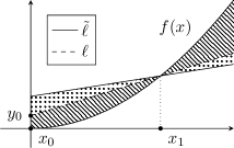
Figure 1: Main idea of proof of Proposition 17

∎

The above statement may be combined with the characterisation of how Beta distributions are ordered according to the star-shaped transform order that was established in the previous section. Doing so allows us to immediately take care of a number of affine $\ell$ in (8).

Corollary 18.

Let $F$ and $G$ be the distribution functions of $\operatorname{Beta}(a,b)$ and $\operatorname{Beta}(a^{\prime},b^{\prime})$, respectively, and assume that $a\geq a^{\prime}$ and $b\leq b^{\prime}$. If $\ell$ is decreasing or satisfies either $\ell(0)\geq 0$ or $\ell(1)\not\in(0,1)$ then (8) is satisfied.

Proof.

We have that (8) holds when $\ell$ is non-increasing, since otherwise $F(x)-G(\ell(x))$ is non-decreasing and so $S(F(x)-G(\ell(x)))\leq\sminus\splus$. Therefore assume $\ell$ is increasing and consider three different cases.

Case 1. $\ell(0)\geq 0$:

According to Theorem 2 and Proposition 27, we have that, for any $c\in\mathbb{R}$, $S(F(x)-G(cx))\leq\sminus\splus$. Taking into account Proposition 17, this implies $S(F(x)-G(\ell(x)))\leq\sminus\splus\leq\splus\sminus\splus$.

Case 2. $\ell(1)\leq 0$:

In this case $\ell$ is always negative, and the result is immediate.

Case 3. $\ell(1)\geq 1$:

It is enough to prove that $S(F(x)-G(c(x-1)+1))\leq\splus\sminus$ for every $c\in\mathbb{R}$. Indeed, once this proved, the conclusion follows using Proposition 17 again.

Note that $F_{-}(x)=1-F(1-x)$ is the distribution function of $\operatorname{Beta}(b,a)$ and $G_{-}(x)=1-G(1-x)$ is the distribution function of $\operatorname{Beta}(b^{\prime},a^{\prime})$. The characterisation of star-shape transform order proved in Theorem 2 together with Proposition 27, means that $S(1-G(1-x)-1+F(1-c^{\prime}x))\leq\sminus\splus$, for every $c^{\prime}\in\mathbb{R}$. For any $c\in\mathbb{R}$ we may apply this to $c^{\prime}=1/c$, which gives

$$\begin{split}S(F(x)-G(c(x-1)+1))&=S(1-G(c(x-1)+1)-1+F(x))\\ &=\operatorname{rev}S(1-G(1-x)-1+F(1-x/c))\\ &\leq\operatorname{rev}(\sminus\splus)=\splus\sminus.\end{split}$$

∎

The proof of Theorem 3, establishing the convex transform ordering within the Beta family is achieved through the analysis of several partial cases. For improved readability we will be presenting these in several lemmas.

Lemma 19.

Let $X\sim\operatorname{Beta}(a,b)$ and $Y\sim\operatorname{Beta}(1,b)$ for some $a\geq 1$ and $b>0$. Then $X\mathrel{\leq_{c}}Y$.

Proof.

Let $F$ and $G$ be the distribution functions of the $\operatorname{Beta}(a,b)$ and $\operatorname{Beta}(1,b)$ distributions, respectively, and $f$ and $g$ their densities. Taking into account Proposition 27 and Corollary 18, we need to show that, for every increasing affine function $\ell(x)=cx+d$ satisfying $\ell(0)=d<0$ and $\ell(1)=c+d\in(0,1)$ one has that (8) is satisfied. We need to separate the arguments into three cases.

Case 1. $b=1$:

In this case the statement follows directly from the convexity of $F(x)=x^{a}$ and that $G(x)=x$.

Case 2. $b\in(0,1)$:

Applying Lemma 14 we have $I=(-d/c,1)$, $\sigma_{1}=\splus$, and $\sigma_{2}\in\{\snull,\sminus,\splus\}$, meaning (5) gives

$$S(F(x)-G(\ell(x)))\leq\splus\cdot\sigma_{2}\cdot S\left(\frac{a-1}{x}-\frac{b-1}{1-x}+\frac{c(b-1)}{1-\ell(x)}\right).$$

But since for $x\in I$

$$\frac{a-1}{x}-\frac{b-1}{1-x}+\frac{c(b-1)}{1-\ell(x)}=\frac{a-1}{x}+\frac{(1-b)(1-(c+d))}{(1-x)(1-\ell(x))}>0,$$

we have $S(F(x)-G(\ell(x)))\leq\splus\cdot\sigma_{2}\cdot\splus\leq\splus\sminus\splus$ no matter the value of $\sigma_{2}$.

Case 3. $b>1$:

Applying Lemma 14 we have $\sigma_{1}=\splus$ and $\sigma_{2}\in\{\snull,\sminus,\splus\}$, meaning (6) gives

$$\begin{split}S(F(x)-G(\ell(x)))&\leq\splus\cdot\sigma_{2}\cdot S(c_{3}x^{3}+c_{2}x^{2}+c_{1}x+c_{0})\\ &=\splus\cdot\sigma_{2}\cdot S(\ell(x)(c^{\prime}_{2}x^{2}+c^{\prime}_{1}x+c^{\prime}_{0}))\\ &=\splus\cdot\sigma_{2}\cdot S(c^{\prime}_{2}x^{2}+c^{\prime}_{1}x+c^{\prime}_{0})\end{split}$$

where $c^{\prime}_{2}=(a-1)c$, $c^{\prime}_{1}=-(a-b)c-(a+b-2)(1-d)$, and $c^{\prime}_{0}=(a-1)(1-d)$. Since $c^{\prime}_{2}>0$ we have $S(c^{\prime}_{2}x^{2}+c^{\prime}_{1}x+c^{\prime}_{0})\leq\splus\sminus\splus$. On the other hand, $c^{\prime}_{2}+c^{\prime}_{1}+c^{\prime}_{0}=-(b-1)(1-(c+d))<0$, hence $S(c^{\prime}_{2}x^{2}+c^{\prime}_{1}x+c^{\prime}_{0})\leq\splus\sminus$. Combining these inequalities yields

$$S(F(x)-G(\ell(x)))\leq\splus\cdot\sigma_{2}\cdot\splus\sminus\leq\splus\sminus\splus\sminus.$$

Finally, as $F(1)-G(\ell(1))>0$, it follows that $S(F(x)-G(\ell(x)))\leq\splus\sminus\splus$.

So, taking into account Proposition 27, the proof is concluded. ∎

The second lemma is similar but covers the case where $a\geq 1$.

Lemma 20.

Let $X\sim\operatorname{Beta}(1,b)$ and $Y\sim\operatorname{Beta}(a,b)$ with $a\leq 1$ and $b>0$. Then $X\mathrel{\leq_{c}}Y$.

Proof.

Let $F$ and $G$ represent the distribution functions of $\operatorname{Beta}(1,b)$ and $\operatorname{Beta}(a,b)$, respectively. Note that the meaning of the symbols $F$ and $G$ are interchanged relative to their use in the proof of Lemma 19. Taking into account Proposition 27 and Corollary 18, we need to show that (8) holds for $\ell(x)=cx+d$ such that $\ell(0)=d<0$ and $\ell(1)=c+d\in(0,1)$. This is equivalent to $S(G(x)-F(\ell^{-1}(x)))\leq\sminus\splus\sminus$, where $\ell^{-1}(x)=(x-d)/c$ satisfies $\ell^{-1}(0)\in(0,1)$ and $\ell^{-1}(1)>1$.

Reversing the roles of $F$ and $G$ the proof is now analogous to that of Lemma 19 except that $a<1$ and we wish to establish $S(x\in I\mapsto G(x)-F(\ell^{\ast}(x)))\leq\sminus\splus\sminus$ for $\ell^{\ast}(x)=c^{\ast}x+d^{\ast}$ with $\ell^{\ast}(0)=d^{\ast}\in(0,1)$ and $\ell^{\ast}(1)=c^{\ast}+d^{\ast}>1$ on the interval $I=(0,(1-d^{\ast})/c^{\ast})$. ∎

Comparing the distributions for more general pairs of parameters $a$ and $a^{\prime}$ requires separate analyses depending on whether $b>1$ or $b\in(0,1)$.

Lemma 21.

Let $X\sim\operatorname{Beta}(a,b)$ and $Y\sim\operatorname{Beta}(a^{\prime},b)$ with $a>a^{\prime}$ and $b>1$. Then $X\mathrel{\leq_{c}}Y$.

Proof.

Let $F$ and $G$ be the distribution functions of $\operatorname{Beta}(a,b)$ and $\operatorname{Beta}(a^{\prime},b)$. By Proposition 27 and Corollary 18, it is enough to prove that (8) holds when $\ell(x)=cx+d$ is such that $\ell(0)=d<0$, $\ell(1)=c+d\in(0,1)$.

Applying Lemma 14 we have $c_{3}=(a-a^{\prime})c^{2}$, $\sigma_{1}=\splus$, and $\sigma_{2}\in\{\snull,\sminus,\splus\}$, meaning (6) gives

$$S(F(x)-G(\ell(x)))\leq\splus\cdot\sigma_{2}\cdot S(c_{3}x^{3}+c_{2}x^{2}+c_{1}x^{1}+c_{0}).$$

Since $c_{3}>0$ we have $S(c_{3}x^{3}+c_{2}x^{2}+c_{1}x^{1}+c_{0})\leq\sminus\splus\sminus\splus$. But $c_{3}+c_{2}+c_{1}+c_{0}=-(b-1)(c+d)(1-(c+d))<0$ so $S(c_{3}x^{3}+c_{2}x^{2}+c_{1}x^{1}+c_{0})\leq\sminus\splus\sminus$.

Combining the sign pattern inequalities, we have derived that

$$S(x\in I\mapsto F(x)-G(\ell(x)))\leq\splus\cdot\sigma_{2}\cdot\sminus\splus\sminus=\splus\sminus\splus\sminus,$$

regardless of the value of $\sigma_{2}$. Finally $F(1)-G(\ell(1))>0$ so we conclude that $S(x\in I\mapsto F(x)-G(\ell(x)))\leq\splus\sminus\splus$, hence proving the result. ∎

Lemma 22.

Let $X\sim\operatorname{Beta}(a,b)$ and $Y\sim\operatorname{Beta}(a^{\prime},b)$ with $0<b\leq 1$ and either $1>a>a^{\prime}>0$ or $a>a^{\prime}>1$. Then $X\mathrel{\leq_{c}}Y$.

Proof.

We may assume, without loss of generality, that $a-a^{\prime}<1$. Indeed, if $a-a^{\prime}\geq 1$, one may choose for sufficiently large $N$ a sequence $a_{0}=a,a_{1},\dotsc,a_{N}=a^{\prime}$ such that $a_{i_{1}}-a_{i}<1$ for all $i=1,\dotsc,N$ and apply transitivity to conclude $\operatorname{Beta}(a_{0},b)\mathrel{\leq_{c}}\dotsb\mathrel{\leq_{c}}\operatorname{Beta}(a_{N},b)$. Let $F$ and $G$ be the distribution functions of $\operatorname{Beta}(a,b)$ and $\operatorname{Beta}(a^{\prime},b)$, respectively. Based on Proposition 27 and Corollary 18, it is enough to prove that (8) holds for every $\ell(x)=cx+d$ such that $\ell(0)=d<0$ and $\ell(1)=c+d\in(0,1)$. Using Lemma 14 we have for $I=(-d/c,1)$ that

$$\begin{split}&S(x\in[0,1]\mapsto F(x)-G(\ell(x)))\\ &\quad\leq\splus\cdot S\left(x\in I\mapsto\frac{x^{a-1}(1-x)^{b-1}}{\operatorname{B}(a,b)}-\frac{\ell(x)^{a^{\prime}-1}(1-\ell(x))^{b-1}}{\operatorname{B}(a^{\prime},b)}\right)\\ &\quad=\splus\cdot S\left(x\in I\mapsto\frac{x^{a-1}}{\ell(x)^{a^{\prime}-1}}-\frac{c\operatorname{B}(a,b)}{\operatorname{B}(a^{\prime},b^{\prime})}\Bigl{(}\frac{1-\ell(x)}{1-x}\Bigr{)}^{b-1}\right).\end{split}$$ (9)

For convenience define $C=c\operatorname{B}(a,b)/\operatorname{B}(a^{\prime},b^{\prime})>0$, $q_{1}(x)=x^{a-1}/\ell(x)^{a^{\prime}-1}$, $q_{2}(x)=(1-x)/(1-\ell(x))$, and $q(x)=q_{1}(x)-Cq_{2}(x)^{1-b}$. Restricting to $I$ we have that $q_{2}$ is decreasing and concave. Hence, as $b\leq 1$, it follows that $x\in I\mapsto-Cq_{2}(x)^{1-b}$ is non-decreasing and convex.

A simple computation yields $q^{\prime}_{1}(x)=((a-a^{\prime})cx+(a-1)d)/(x^{2-a}\ell(x)^{a^{\prime}})$ which has unique root at $x_{0}=-(a-1)d/((a-a^{\prime})c)$. Letting $c_{2}^{\ast}=(a-a^{\prime})(a-a^{\prime}-1)c^{2}$, $c_{1}^{\ast}=2(a-a^{\prime}-1)(a-1)cd$, $c_{0}^{\ast}=(a-1)(a-2)d^{2}$, and $p(x)=c_{2}^{\ast}x^{2}+c_{1}^{\ast}x+c_{0}^{\ast}$ it follows that $q_{1}^{\prime\prime}(x)=p(x)/(x^{3-a}\ell(x)^{a^{\prime}+1})$.

Case 1. $1>a>a^{\prime}$:

In this case $(a-a^{\prime})cx+(a-1)d>0$ for $x>0$, which implies that $q_{1}$ is increasing on $I$. Therefore $x\in I\mapsto q_{1}(x)-Cq_{2}(x)^{1-b}$ is increasing, meaning $S(x\in I\mapsto q_{1}(x)-Cq_{2}(x)^{1-b})\leq\sminus\splus$. Plugged into (9) this gives $S(F(x)-G(\ell(x)))\leq\splus\sminus\splus$.

Case 2. $a>a^{\prime}>1$:

A direct verification shows that $x_{0}\in I$ so that $I_{1}=(-d/c,x_{0}]$ and $I_{2}=(x_{0},1)$ are well defined and non-empty. Since $I=I_{1}\cup I_{2}$ and $I_{1}<I_{2}$

$$S(x\in I\mapsto q(x))=S(x\in I_{1}\mapsto q(x))\cdot S(x\in I_{2}\mapsto q(x)).$$

Sign pattern in $I_{1}$:

As $c_{2}^{\ast}=(a-a^{\prime})(a-a^{\prime}-1)c^{2}<0$ it follows that $S(x\in I\mapsto q_{1}^{\prime\prime}(x))=S(x\in I\mapsto p(x))\leq\sminus\splus\sminus$. But $p(-d/c)=(a^{\prime}-1)a^{\prime}d^{2}>0$ and $p(x_{0})=(a-1)(a^{\prime}-1)d^{2}/(a-a^{\prime})>0$ so $S(x\in I\mapsto p(x))=\splus$.

This implies that $q_{1}$ is convex in $I_{1}$. As we have proved the convexity of $-Cq_{2}(x)^{1-b}$ in $I$, it follows that $q(x)=q_{1}(x)-Cq_{2}(x)^{1-b}$ is convex in $I_{1}$. According to Proposition 26 it follows that

$$S(x\in I_{1}\mapsto q(x))\leq\splus\sminus\splus.$$

Sign pattern in $I_{2}$:

Noting that $S(x\in I\mapsto q_{1}^{\prime}(x))=S((a-a^{\prime})cx+(a-1)d)\leq\sminus\splus$ and $q_{1}^{\prime}(x_{0})=0$, it follows that $q_{1}^{\prime}$ is positive in $I_{2}$. Thus $q_{1}$ is increasing in $I_{2}$. We have proved above that $x\in I\mapsto-Cq_{2}(x)^{1-b}$ is increasing, so $q(x)$ is increasing in the interval $I_{2}$. Therefore

$$S(x\in I_{2}\mapsto q(x))\leq\sminus\splus.$$

If $q(x_{0})<0$ then $S(x\in I_{1}\mapsto q(x))\leq\splus\sminus$. If $q(x_{0})\geq 0$ then $S(x\in I_{2}\mapsto q(x))=\splus$ since $q$ is increasing on $I_{2}$. In either case $S(x\in I_{1}\mapsto q(x))\cdot S(x\in I_{2}\mapsto q(x))\leq\splus\sminus\splus$.

Putting the above into (9) we have

$$S(x\in I\mapsto F(x)-G(\ell(x)))\leq\splus\cdot\splus\sminus\splus=\splus\sminus\splus$$

as required.

∎

We now state, without proof, a straightforward result, helpful for the conclusion of the final characterisation within the $\operatorname{Beta}$ family.

Proposition 23.

Let $X\sim P$ and $Y\sim Q$ be random variables with some distributions $P$ and $Q$, then $X\mathrel{\leq_{c}}Y$ if and only if $1-Y\mathrel{\leq_{c}}1-X$.

We now have all the necessary ingredients to prove the main theorem.

Proof of Theorem 3.

The necessity is a direct consequence of Theorem 1. The sufficiency follows from Lemmas 19, 20, 21, 22, and the transitivity of the convex transform order. First note that we obtain

$$\operatorname{Beta}(a,b)\mathrel{\leq_{c}}\operatorname{Beta}(a^{\prime},b),$$ (10)

when $a=a^{\prime}$ (trivial), $b>1$ (use Lemma 21), $b\leq 1$ and either $1>a>a^{\prime}$ or $a>a^{\prime}>1$ (use Lemma 22). The order relation (10) also holds if $b\leq 1$ and $a>1>a^{\prime}$ by combining Lemmas 19 and 20, since then $\operatorname{Beta}(a,b)\mathrel{\leq_{c}}\operatorname{Beta}(1,b)\mathrel{\leq_{c}}\operatorname{Beta}(a^{\prime},b)$. Using this and Proposition 23 we also have $\operatorname{Beta}(a^{\prime},b)\mathrel{\leq_{c}}\operatorname{Beta}(a^{\prime},b^{\prime})$, concluding the proof. ∎

Appendix A An algebra for sign variation

The main tool of all proofs concerning the ordering within the $\operatorname{Beta}$ family is the study of sign patterns of functions. While such techniques have a long tradition in probability theory, for our purposes it turns out to be computationally convenient to give a presentation slightly more algebraic as compared to what appears to be the convention, using a suitable monoid (see, for example, [14]).

Definition.

Let $(\mathcal{S},\cdot)=\langle\splus,\sminus\mid\splus\cdot\splus=\splus,\sminus\cdot\sminus=\sminus\rangle$ be the monoid generated by two idempotent elements $\splus$ and $\sminus$ and with unit $\snull$.

We shall call elements of $\mathcal{S}$ sign patterns. When unambiguous we will denote products $\sigma\cdot\sigma^{\prime}$ by simply juxtaposing the factors as in $\sigma\sigma^{\prime}$, so that $\mathcal{S}=\{\snull,\splus,\sminus,\splus\sminus,\sminus\splus,\splus\sminus\splus,\dotsc\}$.

For any $\sigma=\sigma_{1}\dotsb\sigma_{n}\in\mathcal{S}$ where $\sigma_{1},\dotsc,\sigma_{n}\in\{\splus,\sminus\}$ let $\operatorname{rev}\sigma=\sigma_{n}\dotsb\sigma_{1}$ be the sign pattern given by reversing the order of signs and let

$$\overline{\sigma}=\overline{\sigma_{0}}\cdot\dotsb\cdot\overline{\sigma_{n}},\qquad\text{where}\qquad\overline{\sigma_{i}}=\begin{cases}\splus&\sigma_{i}=\sminus,\\ \sminus&\sigma_{i}=\splus,\end{cases}$$

denote the sign pattern given by flipping the signs. Note in particular that $\overline{\snull}=\snull$. These operations are well defined on the free monoid generated by $\splus$ and $\sminus$. Since $\operatorname{rev}(\snull)=\snull$, $\overline{\snull}=\snull$, $\operatorname{rev}(\sigma_{1}\dotsb\sigma_{n}\cdot\sigma_{n+1})=\sigma_{n+1}\cdot\operatorname{rev}(\sigma_{1}\dotsb\sigma_{n})$, and $\overline{\sigma_{1}\dotsb\sigma_{n}\cdot\sigma_{n+1}}=\overline{\sigma_{1}\dotsb\sigma_{n}}\cdot\overline{\sigma_{n+1}}$ it follows by a simple induction argument that they are well defined also as operations on $\mathcal{S}$.

Sign patterns have a natural order structure.

Definition.

Given $\sigma,\sigma^{\prime}\in\mathcal{S}$ we say that $\sigma\leq\sigma^{\prime}$ if $\sigma^{\prime}=\pi\cdot\sigma\cdot\pi^{\prime}$ for some $\pi,\pi^{\prime}\in\mathcal{S}$.

Intuitively $\sigma\leq\sigma^{\prime}$ says that $\sigma$ may be written as a substring of $\sigma^{\prime}$.

Proposition 24.

$(\mathcal{S},\cdot,\leq)$ is a partially ordered monoid in the sense that $(\mathcal{S},\leq)$ is a partially ordered set and if $\sigma,\sigma^{\prime}\in\mathcal{S}$ are such that $\sigma\leq\sigma^{\prime}$ then for any $\pi,\pi^{\prime}\in\mathcal{S}$ one has $\pi\cdot\sigma\cdot\pi^{\prime}\leq\pi\cdot\sigma^{\prime}\cdot\pi^{\prime}$.

We can now describe the sign variations of a function in terms of the simple sign function.

Definition (Sign function).

The sign function $\operatorname{Sign}\colon\mathbb{R}\to\mathcal{S}$ is defined by $\operatorname{Sign}(x)=\splus$ if $x>0$, $\operatorname{Sign}(x)=\snull$ if $x=0$, and $\operatorname{Sign}(x)=\sminus$ if $x<0$.

Definition (Sign patterns and finite sign variation).

Given $I\subseteq\mathbb{R}$, we say that a function $f\colon I\mapsto\mathbb{R}$ is of finite sign variation if the set

$$\left\{\operatorname{Sign}(f(x_{1}))\cdot\operatorname{Sign}(f(x_{2}))\cdot\dotsb\cdot\operatorname{Sign}(f(x_{n}))\mid n\in\mathbb{N},x_{1}\leq\dotsb\leq x_{n}\in I\right\}$$

has a (unique) maximal element in $\mathcal{S}$. This maximal element is then denoted by $S(x\in I\mapsto f(x))$ and called the sign pattern of $f$.

When unambiguous, we will abbreviate $S(x\in I\mapsto f(x))=S(x\mapsto f(x))=S(f(x))=S(f)$ and write for readability $\overline{S}(f)=\overline{S(f)}$.

The proposition below gives some standard rules of calculation for sign patterns which are straightforward to prove and used without explicit mention throughout the proofs.

Proposition 25.

Let $I\subset\mathbb{R}$ and $f,g\colon I\to\mathbb{R}$ be such that $f$ and $f-g$ are of finite sign variation.

1. For any $J\subset I$ one has $S(x\in J\mapsto f(x))\leq S(x\in I\mapsto f(x))$.

2. For any $J\leq K$ such that $I=J\cup K$ one has $S(x\in I\mapsto f(x))=S(x\in J\mapsto f(x))\cdot S(x\in K\mapsto f(x))$.

3. For any positive $h\colon I\to\mathbb{R}$ one has $S(f(x))=S(f(x)h(x))$.

4. For $J\subset\mathbb{R}$ and $\eta\colon J\to I$ increasing (or decreasing) one has $S(x\in I\mapsto f(x))=S(x\in J\mapsto f(\eta(x)))$ (respectively $=\operatorname{rev}S(x\in J\mapsto f(\eta(x)))$).

5. For $J\subset f(I)\cup g(I)$ and $\eta\colon J\to\mathbb{R}$ increasing (or decreasing) one has $S(f(x)-g(x))=S(\eta(f(x))-\eta(g(x)))$ (respectively $=\overline{S}(\eta(f(x))-\eta(g(x)))$).

Sign patterns provide a useful tool for establishing convexity or star-shapedness of functions (see for example Lemma 11 and Theorem 20 in [5]).

Proposition 26.

A continuous function $f$ is convex (respectively, star-shaped) if and only if $S(f(x)-\ell(x))\leq\splus\sminus\splus$ (respectively, $S(f(x)-\ell(x))\leq\sminus\splus$), for all affine functions $\ell$ (respectively, for all affine functions $\ell$ vanishing at 0).

Applied to the convex (ifr) and star-shape transform (ifra) orders, these characterisations translate into the following equivalent conditions for being ordered.

Proposition 27.

Let $X$ and $Y$ be random variables with distributions given by distribution functions $F$ and $G$, respectively. Then $X\mathrel{\leq_{c}}Y$ (respectively $X\mathrel{\leq_{\ast}}Y$) if and only if $S(F(x)-G(\ell(x)))\leq\splus\sminus\splus$ (resp., $S(F(x)-G(\ell(x)))\leq\sminus\splus$) for every affine function $\ell$ (resp., for every affine function $\ell$ vanishing at 0).

The following slight generalisation of a well-known relationship between the sign pattern of a differentiable function and the sign pattern of its derivative is also used throughout our proofs.

Proposition 28.

Let $f\colon I\mapsto\mathbb{R}$ be continuously differentiable with finite sign pattern $S(x\in I\to f(x))=\sigma\dotsb$, then $S(x\in I\to f(x))\leq\sigma\cdot S(x\in I\to f^{\prime}(x))$.

Proof.

Let $S(x\in I\to f(x))=\sigma_{0}\sigma_{1}\dotsb\sigma_{n}$. Therefore there exists a sequence $x_{0}<x_{1}<\dotsb<x_{n}$ with $\operatorname{Sign}(f(x_{i}))=\sigma_{i}$. By the mean value theorem there exist $y_{1},\dotsc,y_{n}$ such that $f^{\prime}(y_{i})=(f(x_{i})-f(x_{i-1}))/(x_{i}-x_{i-1})$. Since, in particular, $\operatorname{Sign}(f^{\prime}(y_{i}))=\sigma_{i}$, we have that $\sigma_{1}\dotsb\sigma_{n}\leq S(x\in I\to f^{\prime}(x))$. ∎

If in the statement of Proposition 28 the initial sign of $S(x\in I\to f^{\prime}(x))$ is the same as $\sigma$ the inequality becomes $S(x\in I\to f(x))\leq S(x\in I\to f^{\prime}(x))$. This becomes particularly useful in combination with the following, elementary, proposition.

Proposition 29.

For $b>a$ let $f\colon[a,b]\mapsto\mathbb{R}$ be a continuously differentiable function with finite sign patterns $S(x\in I\to f(x))=\sigma\dotsb\sigma^{\prime}$ and $S(x\in I\to f^{\prime}(x)))=\tau\dotsb\tau^{\prime}$. If $f(a)=0$ then $\sigma=\tau$ and if $f(b)=0$ then $\sigma^{\prime}=\overline{\tau}^{\prime}$.

The interval $[a,b]$ may be replaced by $(a,b]$, $[a,b)$ or $(a,b)$ if the conditions $f(a)=0$ and $f(b)=0$ are replaced by $\lim_{x\to a+}f(x)=0$ or $\lim_{x\to b-}f(x)=0$, as appropriate.

References

- [1] Karim M. Abadir “The Mean-Median-Mode Inequality: Counterexamples” In Econometric Theory 21.2 Cambridge University Press, 2005, pp. 477–482
- [2] A.A. Alzaid and M. Al-Osh “Ordering probability distributions by tail behavior” In Statistics & Probability Letters 8.2, 1989, pp. 185–188
- [3] Idir Arab, Milto Hadjikyriakou and Paulo Eduardo Oliveira “Failure rate properties of parallel systems” In Advances in Applied Probability 52.2 Cambridge University Press, 2020, pp. 563–587
- [4] Idir Arab, Milto Hadjikyriakou and Paulo Eduardo Oliveira “Non comparability with respect to the convex transform order with applications” In Journal of Applied Probability 57 Cambridge University Press, 2020
- [5] Idir Arab and Paulo Eduardo Oliveira “Iterated Failure Rate Monotonicity and Ordering Relations within Gamma and Weibull Distributions” In Probability in the Engineering and Informational Sciences 33.1 Cambridge University Press, 2019, pp. 64–80
- [6] Idir Arab and Paulo Eduardo Oliveira “Iterated Failure Rate Monotonicity and Ordering Relations within Gamma and Weibull Distributions – Corrigendum” In Probability in the Engineering and Informational Sciences 32.4 Cambridge University Press, 2018, pp. 640–641
- [7] Antonio Arriaza, Félix Belzunce and Carolina Martínez-Riquelme “Sufficient conditions for some transform orders based on the quantile density ratio” In Methodology and Computing in Applied Probability (to appear), 2019 DOI: 10.1007/s11009-019-09740-6
- [8] Richard Eugene Barlow, Albert W. Marshall and Frank Proschan “Some inequalities for starshaped and convex functions” In Pacific Journal of Mathematics 29.1 Mathematical Sciences Publishers, 1969, pp. 19–42
- [9] Luca Becchetti, Andrea Clementi, Emanuele Natale, Francesco Pasquale, Riccardo Silvestri and Luca Trevisan “Simple dynamics for plurality consensus” In Distributed Computing 30.4, 2017, pp. 293–306
- [10] Félix Belzunce, José F. Pinar, José M. Ruiz and Miguel A. Sordo “Comparison of concentration for several families of income distributions” In Statistics and Probability Letters 83, 2013, pp. 1036–1045
- [11] Corinna Cortes, Yishay Mansour and Mehryar Mohri “Learning Bounds for Importance Weighting” In Advances in Neural Information Processing Systems 23 Curran Associates, Inc., 2010, pp. 442–450
- [12] Benjamin Doerr “An elementary analysis of the probability that a binomial random variable exceeds its expectation” In Statistics & Probability Letters 139, 2018, pp. 67–74
- [13] Spencer Greenberg and Mehryar Mohri “Tight lower bound on the probability of a binomial exceeding its expectation” In Statistics & Probability Letters 86, 2014, pp. 91–98
- [14] Nathan Jacobson “Basic Algebra I” New York: W. H. FreemanCompany, 1985
- [15] Jongwoo Jeon, Subhash Kochar and Chul Gyu Park “Dispersive ordering–Some applications and examples” In Statistical Papers 47.2, 2006, pp. 227–247
- [16] M.C. Jones “The complementary beta distribution” In Journal of Statistical Planning and Inference 104.2, 2002, pp. 329–337
- [17] Matti Karppa, Petteri Kaski and Jukka Kohonen “A Faster Subquadratic Algorithm for Finding Outlier Correlations” In ACM Transactions on Algorithms 14.3 New York, NY, USA: Association for Computing Machinery, 2018
- [18] Bernd Lisek “Comparability of special distributions” In Series Statistics 9.4 Taylor & Francis, 1978, pp. 587–598
- [19] Albert W. Marshall and Ingram Olkin “Life Distributions: Structure of Nonparametric, Semiparametric, and Parametric Families” New York, NY: Springer New York, 2007
- [20] Michael Mitzenmacher and Tom Morgan “Reconciling Graphs and Sets of Sets” In Proceedings of the 37th ACM SIGMOD-SIGACT-SIGAI Symposium on Principles of Database Systems, SIGMOD/PODS ’18 Houston, TX, USA: Association for Computing Machinery, 2018, pp. 33–47
- [21] Asok K. Nanda, Nil Kamal Hazra, Dhaifalla K. Al-Mutairi and Mohamed E. Ghitany “On some generalized ageing orderings” In Communications in Statistics - Theory and Methods 46.11 Taylor & Francis, 2017, pp. 5273–5291
- [22] Hannu Oja “On Location, Scale, Skewness and Kurtosis of Univariate Distributions” In Scandinavian Journal of Statistics 8.3 Wiley, 1981, pp. 154–168
- [23] Emanuel Parzen “Nonparametric Statistical Data Modeling” In Journal of the American Statistical Association 74.365 Taylor & Francis, 1979, pp. 105–121
- [24] Christos Pelekis “Lower bounds on binomial and Poisson tails: an approach via tail conditional expectations” In arXiv preprin arXiv:1609.06651, 2016 arXiv:1609.06651 [math.PR]
- [25] Christos Pelekis and Jan Ramon “A lower bound on the probability that a binomial random variable is exceeding its mean” In Statistics & Probability Letters 119, 2016, pp. 305–309
- [26] J.. Runnenburg “Mean, median, mode” In Statistica Neerlandica 32.2, 1978, pp. 73–79
- [27] Moshe Shaked and Jeyaveerasingam George Shanthikumar “Stochastic Orders”, Springer Series in Statistics Springer New York, 2007
- [28] Tilo Wiklund “The Deficiency Introduced by Resampling” In Mathematical Methods of Statistics 27.2, 2018, pp. 145–161
- [29] Shimin Zheng, Eunice Mogusu, Sreenivas P. Veeranki, Megan Quinn and Yan Cao “The relationship between the mean, median, and mode with grouped data” In Communications in Statistics - Theory and Methods 46.9 Taylor & Francis, 2017, pp. 4285–4295
- [30] Willem Rutger Zwet “Convex transformations of random variables”, Mathematical Centre tracts Mathematisch Centrum, 1964
- [31] Willem Rutger Zwet “Mean, median, mode II” In Statistica Neerlandica 33.1, 1979, pp. 1–5