Cyclic stratum of Frobenius manifolds, Borel-Laplace $(\boldsymbol{\alpha},\boldsymbol{\beta})$-multitransforms, and integral representations of solutions of Quantum Differential Equations

Abstract.

In the first part of this paper, we introduce the notion of cyclic stratum of a Frobenius manifold $M$. This is the set of points of the extended manifold ${\mathbb{C}}^{*}\times M$ at which the unit vector field is a cyclic vector for the isomonodromic system defined by the flatness condition of the extended deformed connection. The study of the geometry of the complement of the cyclic stratum is addressed. We show that at points of the cyclic stratum, the isomonodromic system attached to $M$ can be reduced to a scalar differential equation, called the master differential equation of $M$. In the case of Frobenius manifolds coming from Gromov-Witten theory, namely quantum cohomologies of smooth projective varieties, such a construction reproduces the notion of quantum differential equation.

In the second part of the paper, we introduce two multilinear transforms, called Borel-Laplace $(\boldsymbol{\alpha},\boldsymbol{\beta})$-multitransforms, on spaces of Ribenboim formal power series with exponents and coefficients in an arbitrary finite dimensional ${\mathbb{C}}$-algebra $A$. When $A$ is specialized to the cohomology of smooth projective varieties, the integral forms of the Borel-Laplace $(\boldsymbol{\alpha},\boldsymbol{\beta})$-multitransforms are used in order to rephrase the Quantum Lefschetz Theorem. This leads to explicit Mellin-Barnes integral representations of solutions of the quantum differential equations for a wide class of smooth projective varieties, including Fano complete intersections in projective spaces.

In the third and final part of the paper, as an application, we show how to use the new analytic tools, introduced in the previous parts, in order to study the quantum differential equations of Hirzebruch surfaces. For Hirzebruch surfaces diffeomorphic to ${\mathbb{P}}^{1}\times{\mathbb{P}}^{1}$, this analysis reduces to the simpler quantum differential equation of ${\mathbb{P}}^{1}$. For Hirzebruch surfaces diffeomorphic to the blow-up of ${\mathbb{P}}^{2}$ in one point, the quantum differential equation is integrated via Laplace $(1,2;\frac{1}{2},\frac{1}{3})$-multitransforms of solutions of the quantum differential equations of ${\mathbb{P}}^{1}$ and ${\mathbb{P}}^{2}$, respectively. This leads to explicit integral representations for the Stokes bases of solutions of the quantum differential equations, and finally to the proof of Dubrovin Conjecture for all Hirzebruch surfaces.

1. Introduction

1.1   The Main Problem. We consider the analytic Frobenius manifold defined by the quantum cohomology $QH^{\bullet}(X)$ of a complex smooth projective variety $X$ [Dub96, KM94, Man99]. Points $p\in QH^{\bullet}(X)$ are parameters of isomonodromic deformations of a linear system of differential equations of the form

$$\frac{\partial}{\partial z}\zeta(z,p)=\left(\mathcal{U}(p)+\frac{1}{z}\mu(p)\right)\zeta(z,p).$$ (1.1)

Here $\zeta$ is a $z$-dependent vector field of $QH^{\bullet}(X)$, whereas $\mathcal{U}$ and $\mu$ are $(1,1)$-tensors on $QH^{\bullet}(X)$: the first is the operator of quantum multiplication by the Euler vector field - a distinguished vectof field on $QH^{\bullet}(X)$ which equals the first Chern class $c_{1}(X)$ along the locus of small quantum cohomology - the second, called grading operator, keeps track of the non-vanishing degrees of $H^{\bullet}(X,{\mathbb{C}})$.

Equation (1.1) is a rich object associated with the variety $X$: it encapsulates information not only about its Gromov-Witten theory, but also (conjecturally) about its topology, its algebraic geometry, and their mutual relations. The study of the monodromy of solutions of (1.1) is the way to disclose such an amount of information, see [Dub98, GGI16, CDG18]. In this paper we address the following

Main Problem: to find integral representations of solutions of (1.1) for Fano complete intersections in Fano varieties.

We split the Main Problem in two parts:

1. to reduce the system of differential equations (1.1) to a distinguished scalar linear differential equation, the master differential equation;

2. to find integral representations of solutions of master differential equations.

The study of these questions leads us to introduce some relevant notions, both in the analytic theory of Frobenius manifolds and in the theory of integral transforms. The first three ingredients are the notions of cyclic stratum, master differential equations and master functions of a Frobenius manifold. The second new analytical tool is a pair of integral multilinear transforms of functions, that we call Borel-Laplace $(\boldsymbol{\alpha},\boldsymbol{\beta})$-multitansforms. We are going to briefly outline these objects.

1.2   Master functions and master differential equations. The rich geometry of a Frobenius manifold $M$ is (almost) completely encoded in integrability conditions of the extended deformed connection or first structural connection of $M$ [Dub96, Dub99, Man99]. This is a flat meromorphic connection $\widehat{\nabla}$ defined on the pullback $\pi^{*}TM$ of the tangent bundle of $M$ on the extended manifold $\widehat{M}:={\mathbb{C}}^{*}\times M$, by the natural projection $\pi\colon\widehat{M}\to M$. Equation (1.1) is equivalent to the equation

$$\widehat{\nabla}_{\frac{\partial}{\partial z}}\xi=0,\quad\xi\in\Gamma(\pi^{*}T^{*}M),$$ (1.2)

the one-form $\xi$ and the vector field $\zeta$ being identified via a flat metric $\eta$ on $M$. We call master function at $p\in M$ any function $\Phi_{\xi}\in\mathcal{O}(\widetilde{{\mathbb{C}}^{*}})$ of the form

$$\Phi_{\xi}(z)=z^{-\frac{d}{2}}\langle\xi(z,p),e(p)\rangle,$$

where $\xi$ is as in (1.2), and $d$ is the charge of the Frobenius manifold $M$.

In the first part of the paper, we address the problem of reducing the system of differential equations (1.2) to a scalar differential equation, whose coefficients depend on the point $p\in M$. This is a well known problem in the theory of ordinary differential equations, equivalent to the choice of a cyclic vector [Del70, Lemma II.1.3]. On Frobenius manifold, however, we have a natural candidate, namely the unit vector field $e\in\Gamma(TM)$.

In Section 2 we introduce the cyclic stratum $\widehat{M}^{\rm cyc}\subseteq\widehat{M}$ defined as the set of points $(z,p)$ at which the iterated covariant derivatives

$$e,\quad\widehat{\nabla}_{\frac{\partial}{\partial z}}e,\quad\widehat{\nabla}^{2}_{\frac{\partial}{\partial z}}e,\dots,\quad\widehat{\nabla}^{n-1}_{\frac{\partial}{\partial z}}e,\quad n:=\dim_{\mathbb{C}}M,$$ (1.3)

define a basis of the fiber $\pi^{*}TM|_{(z,p)}$. The complement of $\widehat{M}^{\rm cyc}$ in ${\mathbb{P}}^{1}\times M$ admits a natural stratification, whose study is addressed in Section 2.6. A particular role is played by the $\mathcal{A}_{\Lambda}$-stratum of $M$, defined as the set of points $p\in M$ such that

$${\mathbb{C}}^{*}\times\{p\}\subseteq\widehat{M}\setminus\widehat{M}^{\rm cyc}.$$

Introducing the cyclic coframe $\omega_{0}\dots,\omega_{n-1}\in\Gamma(\pi^{*}T^{*}M)$ as the dual frame of (1.3), the system of differential equations (1.2), specialized at points $p\in M\setminus\mathcal{A}_{\Lambda}$, reduces to a scalar differential equation - the master differential equation - in the function $\langle\xi,e\rangle$. Hence, at points $p\in M\setminus\mathcal{A}_{\Lambda}$, we obtain a one-to-one correspondence

$$\left\{\begin{aligned} &\text{Solutions $\xi$ of the system}\\ &\text{ \eqref{de2} specialized at $p$}\\ \end{aligned}\right\}\Longleftrightarrow\left\{\text{Master functions $\Phi_{\xi}$'s at $p$}\right\}.$$

See Theorems 2.29 and 2.31. Thus, if integral representations for a basis of master functions are found, we can consider solved the Main Problem at points in $M\setminus\mathcal{A}_{\Lambda}$.

Some motivational comments for introducing these new tools are in order. The notions of master functions and master differential equations define analogs, for an arbitrary Frobenius manifold, of well-known objects in Gromov-Witten and quantum cohomology theories. Namely, in the case of quantum cohomology the components of Givental’s $J$-function (w.r.t. an arbitrary cohomology basis) define a generating set of master functions. Moreover, the master differential equation is (up to re-scaling of the unknown function) a quantum differential equation as defined e.g. in [CK99, Section 10.3], see Section 5. In our opinion the concepts of cyclic stratum, master functions, and master differential equations may represent relevant notions in the analytic theory of Frobenius manifolds. We stress e.g. the “experimental” evidence of relations with the geometry of distinguished subsets of Frobenius manifolds: in all the examples considered so far, the $\mathcal{A}_{\Lambda}$-stratum described above coincides with the Maxwell stratum, defined as the closure of the set of semisimple coalescing points. We conjecture that this holds true in general, see Conjecture 2.26. It would be interesting to study relations with results of [CDG19, CDG20], concerning the isomonodromic description of Frobenius manifolds at semisimple coalescing points. This point will be addressed in a future publication.

1.3   Borel-Laplace multitransforms. In Section 6, we introduce a pair of multilinear transforms in both a formal and an analytical setting.

For $h\in{\mathbb{N}}^{*}$, and a given $h$-tuple $\boldsymbol{\kappa}\in({\mathbb{C}}^{*})^{h}$, we introduce a ring $\mathscr{F}_{\boldsymbol{\kappa}}(A)$ of Ribenboim generalized power series [Rib92, Rib94] with both coefficients and exponents in a finite dimensional, commutative, associative, and unitary ${\mathbb{C}}$-algebra $A$. The numbers $\kappa_{i}$’s play a role of “weights” for the exponents of the power series. In such a formal setting, given $\boldsymbol{\alpha},\boldsymbol{\beta}\in({\mathbb{C}}^{*})^{h}$, we introduce the Borel-Laplace $(\boldsymbol{\alpha},\boldsymbol{\beta})$-multitransforms as two $A$-multilinear maps rescaling the weights

$$\mathscr{B}_{\boldsymbol{\alpha},\boldsymbol{\beta}}\colon\bigotimes_{j=1}^{h}\mathscr{F}_{\kappa_{j}}(A)\to\mathscr{F}_{\boldsymbol{\alpha}^{-1}\cdot\boldsymbol{\beta}^{-1}\cdot\boldsymbol{\kappa}}(A), \boldsymbol{\alpha}^{-1}\cdot\boldsymbol{\beta}^{-1}\cdot\boldsymbol{\kappa}:=\left(\frac{\kappa_{1}}{\alpha_{1}\beta_{1}},\dots,\frac{\kappa_{h}}{\alpha_{h}\beta_{h}}\right),$$

$$\mathscr{L}_{\boldsymbol{\alpha},\boldsymbol{\beta}}\colon\bigotimes_{j=1}^{h}\mathscr{F}_{\kappa_{j}}(A)\to\mathscr{F}_{\boldsymbol{\alpha}\cdot\boldsymbol{\beta}\cdot\boldsymbol{\kappa}}(A), \boldsymbol{\alpha}\cdot\boldsymbol{\beta}\cdot\boldsymbol{\kappa}:=(\alpha_{1}\beta_{1}\kappa_{1},\dots,\alpha_{h}\beta_{h}\kappa_{h}).$$

See Sections 6.2 and 6.3 for precise definitions.

In the analytical setting, given $h$ functions $\Phi_{1},\dots,\Phi_{h}\colon\widetilde{{\mathbb{C}}^{*}}\to A$, we define their Borel-Laplace $(\boldsymbol{\alpha},\boldsymbol{\beta})$-multitransforms by

$$\mathscr{B}_{\boldsymbol{\alpha},\boldsymbol{\beta}}[\Phi_{1},\dots,\Phi_{h}](z):=\frac{1}{2\pi i}\int_{\gamma}\prod_{j=1}^{h}\Phi_{j}\left(z^{\frac{1}{\alpha_{j}\beta_{j}}}\lambda^{-\beta_{j}}\right)e^{\lambda}\frac{d\lambda}{\lambda},$$

$$\mathscr{L}_{\boldsymbol{\alpha},\boldsymbol{\beta}}\left[\Phi_{1},\dots,\Phi_{h}\right](z):=\int_{0}^{\infty}\prod_{i=1}^{h}\Phi_{i}(z^{\alpha_{i}\beta_{i}}\lambda^{\beta_{i}})e^{-\lambda}d\lambda,$$

provided that the integrals exist. The contour $\gamma$ is a Hankel-type contour beginning from $-\infty$, circling the origin once in the positive direction, and returing to $-\infty$ (see Figure 6.1).

1.4   Main results. Consider a Fano smooth projective variety $X$, and let $\iota\colon Y\to X$ be a Fano subvariety defined as the zero locus of a regular section of a vector bundle $E\to X$. The classical cohomology groups $H^{k}(Y,{\mathbb{C}})$ can be (partially) recovered by the cohomology groups $H^{k}(X,{\mathbb{C}})$ by Lefschetz Hyperplane Theorem. Quantum Lefschetz Theorem is a quantum improvement of the classical result: it describes how to reconstruct the Gromov-Witten theory of $Y$ starting from the Gromov-Witten theory of $X$ [Lee01, CG07, Coa14].

In this paper, by using Quantum Lefschetz Theorem, we give explicit integral representations of master functions of $Y$ in terms of Laplace $(\boldsymbol{\alpha},\boldsymbol{\beta})$-multitransforms of master functions of the ambient space $X$ under the following assumptions on $X$ and $E$:

1. We assume that $E$ is a direct sum of fractional powers of the determinant bundle $\det TX$ of $X$;

2. We assume that $X=X_{1}\times\dots\times X_{h}$ is a product of Fano varieties $X_{i}$’s, and that $E$ is the external tensor product of fractional powers of the determinant bundles $\det TX_{i}$.

Our first main result concerns Case 1. Our Theorem 7.1 asserts that any master function of $Y$, at points $\iota^{*}\delta\in H^{2}(Y,{\mathbb{C}})$ of its small quantum cohomology, can be expressed in terms of iterated Laplace $(\alpha,\beta)$-transforms (simple transforms of a single function) of master functions of $X$ at the point $\delta\in H^{2}(X,{\mathbb{C}})$. More precisely, if $E=\bigoplus_{j=1}^{r}L^{\otimes d_{j}}$, and $\det TX=L^{\ell}$ for an ample line bundle $L$, then any master function of $Y$ at $\iota^{*}\delta$ is a ${\mathbb{C}}$-linear combination of integrals of the form

$$e^{-c_{\delta}z}\mathscr{L}_{\frac{\ell-\sum_{i=1}^{s}d_{i}}{d_{s}},\frac{d_{s}}{\ell-\sum_{i=1}^{s-1}d_{i}}}\circ\dots\circ\mathscr{L}_{\frac{\ell-d_{1}-d_{2}}{d_{2}},\frac{d_{2}}{\ell-d_{1}}}\circ\mathscr{L}_{\frac{\ell-d_{1}}{d_{1}},\frac{d_{1}}{\ell}}[\Phi]$$

$$=e^{-c_{\delta}z}\int_{0}^{\infty}\dots\int_{0}^{\infty}\Phi\left(z^{\frac{\ell-\sum_{j=1}^{r}d_{j}}{\ell}}\prod_{i=1}^{r}\zeta_{i}^{\frac{d_{i}}{\ell}}\right)e^{-\sum_{i=1}^{r}\zeta_{i}}d\zeta_{1}\dots d\zeta_{r},$$

where $\Phi$ is a master function of $X$ at $\delta$, and $c_{\delta}\in{\mathbb{C}}$ is a complex number depending on $\delta$.

Our second main result concerns Case 2. In particular, Theorem 7.4 asserts that any master function of $Y$, at points $\iota^{*}\delta\in H^{2}(Y,{\mathbb{C}})$ of the small quantum locus, can be expressed in terms of Laplace $(\boldsymbol{\alpha},\boldsymbol{\beta})$-multitransforms of master functions of $X_{j}$ at the point $\delta_{j}\in H^{2}(X,{\mathbb{C}})$, where

$$\delta=\sum_{j=1}^{h}1\otimes\dots\otimes\delta_{j}\otimes\dots\otimes 1.$$

More precisely, if $E=\boxtimes_{j=1}^{h}L_{j}^{\otimes d_{j}}$ and $\det TX_{j}=L_{j}^{\ell_{j}}$ for ample line bundles $L_{j}$, then any master functions of $Y$ at $\iota^{*}\delta$ is a ${\mathbb{C}}$-linear combination of integrals of the form

$$e^{-c_{\delta}z}\mathscr{L}_{\boldsymbol{\alpha},\boldsymbol{\beta}}[\Phi_{1},\dots,\Phi_{h}](z)=e^{-c_{\delta}z}\int_{0}^{\infty}\prod_{j=1}^{h}\Phi_{j}\left(z^{\frac{\ell_{j}-d_{j}}{\ell_{j}}}\lambda^{\frac{d_{j}}{\ell_{j}}}\right)e^{-\lambda}d\lambda,$$

where $(\boldsymbol{\alpha},\boldsymbol{\beta})=(\frac{\ell_{1}-d_{1}}{d_{1}},\dots,\frac{\ell_{h}-d_{h}}{d_{h}};\frac{d_{1}}{\ell_{1}},\dots,\frac{d_{h}}{\ell_{h}})$, $\Phi_{j}$ is a master function of $X_{j}$ at $\delta_{j}$, and $c_{\delta}\in{\mathbb{C}}$ is a complex number depending on $\delta$.

Assumptions of Cases 1 and 2 are clearly satisfied when the varieties $X$ and $X_{j}$’s have Picard rank one. Therefore, Theorems 7.1 and 7.4 can be applied to all Fano complete intersections in ${\mathbb{P}}^{n}$ and Fano hypersurfaces in products of projective spaces, in order to obtain explicit Mellin-Barnes integral representations of master functions. In particular, if $Y\subseteq{\mathbb{P}}^{n-1}$ is a Fano complete intersection defined by homogenous polynomials of degrees $d_{1},\dots,d_{h}$, our Theorem 7.7 asserts that any master function of $Y$ at $0\in H^{\bullet}(Y,{\mathbb{C}})$ is a linear combination of one-dimensional Mellin-Barnes integrals

$$G_{j}(z)=\frac{e^{-cz}}{2\pi\sqrt{-1}}\int_{\gamma}\Gamma(s)^{n}\prod_{k=1}^{h}\Gamma\left(1-d_{k}s\right)z^{-(n-\sum_{k=1}^{h}d_{k})s}\varphi_{j}(s)ds,\quad j=0,\dots,n-1,$$

where $c\in{\mathbb{Q}}$, $\gamma$ is a parabola encircling the poles of the factor $\Gamma(s)^{n}$ and separating them from the poles of the factors $\Gamma\left(1-d_{k}s\right)$, and the function $\varphi_{j}(s)$ are defined by

$$\exp\left({2\pi\sqrt{-1}js}\right),\quad n\text{ even,}$$

$$\exp\left({2\pi\sqrt{-1}js}+\pi\sqrt{-1}s\right),\quad n\text{ odd}.$$

In the case of a Fano hypersurface $Y\subseteq{\mathbb{P}}^{n_{1}-1}\times\dots\times{\mathbb{P}}^{n_{h}-1}$ defined by a homogeneous polynomial of multi-degree $(d_{1},\dots,d_{h})$, then our Theorem 7.8 asserts that any master function of $Y$ at $0\in H^{\bullet}(Y,{\mathbb{C}})$ is a linear combination of the $h$-dimensional Mellin-Barnes integrals

$$H_{\boldsymbol{j}}(z):=\frac{e^{-cz}}{(2\pi\sqrt{-1})^{h}}\int_{\bigtimes\gamma_{i}}\left[\prod_{i=1}^{h}\Gamma(s_{i})^{n_{i}}\varphi_{j_{i}}^{i}(s_{i})\right]\Gamma\left(1-\sum_{i=1}^{h}s_{i}\right)z^{-\sum_{i=1}^{h}d_{i}s_{i}}ds_{1}\dots ds_{h},$$

where $c\in{\mathbb{Q}}$, $\gamma_{j}$ are parabolas encircling the poles of the factors $\Gamma(s_{i})^{n_{i}}$, and the functions $\varphi_{j_{i}}^{i}(s_{i})$ are defined by

$$\exp\left({2\pi\sqrt{-1}j_{i}s_{i}}\right),\quad n_{i}\text{ even},$$

$$\exp\left({2\pi\sqrt{-1}j_{i}s_{i}}+\pi\sqrt{-1}s_{i}\right),\quad n_{i}\text{ odd},$$

for any $h$-tuple $\boldsymbol{j}=(j_{1},\dots,j_{h})$ with $0\leqslant j_{h}\leqslant n_{i}-1$.

Some comments are in order. Given a Fano variety $X$, Mirror Symmetry provides other kinds of integral representations of solutions of equation (1.2). These are complex oscillating integrals associated with the Landau-Ginzburg models mirror to $X$, see [Giv95, Giv97, Giv98, EHX97, Kon98, HV00]. In these representations the cycles of integration are multi-dimensional. This fact typically makes more difficult the study of the aysmptotic expansions of solutions, and of the determination of the corresponding validity sectors in $\widetilde{{\mathbb{C}}^{*}}$. Furthermore, let us recall another technical issue which may be faced: Landau-Ginzburg models may not have enough critical points, and suitable compactification procedures have to be applied in order to recover the right number, see [Rie08, GS15, PR18]. This could represent a delicate point for the computation of the Stokes bases of solutions of equation (1.1), whose exponential growth is ruled by the critical values of the Landau-Ginzburg potential.

We believe that one-dimensional Mellin-Barnes integrals of Theorem 7.7 represent a more advantageous representation of the solutions to the purpose of asymptotic analysis. Moreover, even for multi-dimensional Mellin-Barnes integrals of Theorem 7.8 the study of their asymptotics is tame: it is equivalent to the study of the asymptotics of one-dimensional generalized Faxén integrals

$$I(\lambda;c_{1},\dots,c_{r}):=\int_{0}^{\infty}\exp\left[-\lambda\left(x^{\mu}+\sum_{k=1}^{r}c_{k}x^{m_{k}}\right)\right]d\lambda,$$

$$\text{with }\mu>m_{1}>m_{2}>.\dots>m_{r}>0,$$

which have saddle points whose exponential contributions dominate algebraic terms in the asymptotic expansion. See [PK01, Chapter 7], [KP97, Section 5] for a detailed asymptotic analysis, and also [Bur24, Bak33, Wri40] for some special cases. This will be exemplified in Section 11.6.

1.5   Dubrovin Conjecture for Hirzebruch surfaces. Equation (1.1) has two singularities: a Fuchsian singularity at $z=0$ and an irregular singularity at $z=\infty$ of Poincaré rank 1. The monodromy of its solutions is quantified by a finite set of matrices:

• a monodromy matrix $M_{0}$, quantifying the monodromy of solutions of (1.1) at $z=0$,

• a Stokes matrix $S$, describing the Stokes phenomenon at $z=\infty$,

• and a central connection matrix $C$ gluing the monodromy data $M_{0}$ and $S$ at the two singularities.

Remarkably, the monodromy data define a sort of “system of coordinates” in the space of solutions of WDVV equations: from the knowledge of their numerical values, the whole Frobenius manifold structure can be reconstructed via a Riemann-Hilbert problem [Dub96, Dub99, Guz01].

In [Dub98], B. Dubrovin formulated an intriguing conjecture concerning the geometrical meaning of the numerical values of the monodromy data of quantum cohomologies of Fano varieties. In the qualitative part of the conjecture, for a given Fano variety $X$, the semisimplicity condition of $QH^{\bullet}(X)$ is claimed to be equivalent to the existence of full exceptional collections in the derived category $\mathcal{D}^{b}(X)$ of coherent sheaves on $X$. Moreover, in the refined quantitative part of the conjecture, formulated in [CDG18, Conjecture 5.2], the Stokes and central connection matrices $(S_{p},C_{p})$ computed at any point $p\in QH^{\bullet}(X)$ are claimed to be determined by characteristic classes of $X$ and of objects of a full exceptional collection $\mathfrak{E}_{p}$ in $\mathcal{D}^{b}(X)$.

In particular, the central connection matrix $C_{p}$ is claimed to equal the matrix associated with the morphism

$$\textnormal{\textcyr{D}}_{X}^{-}\colon K_{0}(X)_{\mathbb{C}}\longrightarrow H^{\bullet}(X,{\mathbb{C}})$$ (1.4)

$$F\xmapsto{\quad\quad} \frac{(\sqrt{-1})^{\overline{d}}}{(2\pi)^{\frac{d}{2}}}\widehat{\Gamma}^{-}_{X}\exp(-\pi\sqrt{-1}c_{1}(X)){\rm Ch}(F),$$

where $d=\dim_{\mathbb{C}}X$, $\overline{d}$ is its residue class modulo 2, $\widehat{\Gamma}^{-}_{X}$ is the characteristic class of $X$ defined by

$$\Gamma^{-}_{X}:=\prod_{j=1}^{\dim_{\mathbb{C}}X}\Gamma(1-\delta_{j}),\quad\Gamma(1-t)=\exp\left(\gamma t+\sum_{n=2}^{\infty}\frac{\zeta(n)}{n}t^{n}\right),\quad\delta_{j}\text{ Chern roots of $TX$,}$$

and ${\rm Ch}(F)$ is the graded Chern character defined on vector bundles by the formula ${\rm Ch}(V):=\sum_{j=1}^{{\rm rk}V}\exp(2\pi\sqrt{-1}\varepsilon_{j})$, $\varepsilon_{j}$’s being the Chern roots of $V$. The matrix of D${}^{-}_{X}$ is computed w.r.t. the exceptional basis $[\mathfrak{E}_{p}]$ of $K_{0}(X)_{{\mathbb{C}}}$, defined by the $K$-theoretical classes of objects of $\mathfrak{E}_{p}$, and an arbitrary basis of $H^{\bullet}(X,{\mathbb{C}})$. Furthermore, if the central connection matrix $C_{p}$ is related to the morphism $\textcyr{D}^{-}_{X}$ as explained above, then the Stokes matrix $S_{p}$ automatically equals the inverse of the Gram matrix of the Grothendieck-Euler-Poincaré $\chi$-pairing on $K_{0}(X)$ w.r.t. the exceptional basis $[\mathfrak{E}_{p}]$, see [CDG18, Corollary 5.8].

It is important to stress that the monodromy data $(M_{0},S,C)$ are defined up to several choices: the choice of a system of flat coordinates on the Frobenius manifold $QH^{\bullet}(X)$, choices of normalizations (at both $z=0$ and $z=\infty$) of solutions of equation (1.1), and the choice of an “admissible ray” in ${\mathbb{C}}^{*}$. Remarkably, all these operations have a geometrical counterpart in derived categories, see [CDG18, Theorem 5.9]. Deserving special mention is $\Gamma$- conjecture II of [GGI16]: it consists of an equivalent conjectural statement about the central connection matrix, though w.r.t. a choice of a solution in “Levelt form” at $z=0$ not natural from the point of view of the theory of Frobenius manifolds. See [CDG18, Section 5.6] for details.

The explicit computation of the monodromy data of quantum cohomologies is typically a rather delicate operation. To the best knowledge of the author, the only cases in which the computation of the complete set of monodromy data $(S,C)$ of equation (1.1) has been carried out in all the details (including the determination of the corresponding full exceptional collections) are the cases of projective spaces [Dub99, Guz99] and of complex Grassmannians [GGI16, CDG18]. We believe that the main results of the current paper, namely the integral representations described in Theorems 7.1, 7.4, 7.7, and 7.8, will represent a fundamental tool for the development of this study [Cot].

As an application, in Sections 10 and 11, we show how to use the Laplace $(\boldsymbol{\alpha},\boldsymbol{\beta})$-multitransform, and the main results described above, in order to prove Dubrovin Conjecture for Hirzebruch surfaces [Hir51]. These are surfaces ${\mathbb{F}}_{k}$, with $k\in{\mathbb{Z}}$, defined as the total space of the projective bundle ${\mathbb{P}}(\mathcal{O}\oplus\mathcal{O}(-k))$ on ${\mathbb{P}}^{1}$. The interest of this example is highlighted by the fact that

• only two Hirzebruch surfaces are Fano varieties (namely ${\mathbb{F}}_{0}$ and ${\mathbb{F}}_{1}$),

• all others Hirzebruch surfaces are deformation equivalent to either ${\mathbb{F}}_{0}$ or ${\mathbb{F}}_{1}$.

Results of A. Bayer already suggested the unnecessity of the Fano assumption for the validity of the qualitative part of Dubrovin Conjecture, see [Bay04]. Moreover, X. Hu proved that, in a smooth family of complete varieties, the existence of full exceptional collection on a fiber preserves for the fibers in a neighborhood, see [Hu18]. See also [BOR20, Corollary B] for an analogue result for arbitrary semiorthogonal decompositions. To the best of our knowledge, the study of the monodromy of the isomonodromic systems (1.1) associated with Hirzebruch surfaces, developed in Sections 10 and 11, represents the first example in literature which addresses also the quantitative part of Dubrovin Conjecture, in both the non-Fano case and the case of deformations of the complex structures.

The case of Hirzebruch surfaces ${\mathbb{F}}_{2k}$ (resp. ${\mathbb{F}}_{2k+1}$) can be reduced to the single case of ${\mathbb{F}}_{0}={\mathbb{P}}^{1}\times{\mathbb{P}}^{1}$ (resp. ${\mathbb{F}}_{1}={\rm Bl}_{pt}{\mathbb{P}}^{2}$). The monodromy data of $QH^{\bullet}({\mathbb{F}}_{0})$ can be easily reconstructed from the monodromy data of $QH^{\bullet}({\mathbb{P}}^{1})$, see Theorem 10.5. In the case of $QH^{\bullet}({\mathbb{F}}_{1})$, the computation is more delicate, and reduces to the study of the quantum differential equation

$$(283z-24)\vartheta^{4}\Phi+\left(283z^{2}-590z+24\right)\vartheta^{3}\Phi+\left(-2264z^{2}+192z+3\right)\vartheta^{2}\Phi\\ -4z^{2}\left(2547z^{2}+350z-104\right)\vartheta\Phi+z^{2}\left(-3113z^{3}-9924z^{2}+1476z+192\right)\Phi=0,$$

where $\vartheta:=z\frac{d}{dz}$. In Section 11.4, we show that the solutions of this equation can be expressed as linear combinations of integrals of the form

$$e^{-z}\mathscr{L}_{(1,2;\frac{1}{2},\frac{1}{3})}[\Phi_{1},\Phi_{2};z]=e^{-z}\int_{0}^{\infty}\Phi_{1}\left(z^{\frac{1}{2}}\lambda^{\frac{1}{2}}\right)\Phi_{2}\left(z^{\frac{2}{3}}\lambda^{\frac{1}{3}}\right)e^{-\lambda}d\lambda,$$

where $\Phi_{1}$ and $\Phi_{2}$ are solutions of quantum differential equations of ${\mathbb{P}}^{1}$ and ${\mathbb{P}}^{2}$ respectively, that is

$$\vartheta^{2}\Phi_{1}=4z^{2}\Phi_{1},\quad\vartheta^{3}\Phi_{2}=27z^{3}\Phi_{2}.$$

This allows the study of the asymptotics of solutions in sectors of $\widetilde{{\mathbb{C}}^{*}}$, to reconstruct the Stokes bases of solutions of the quantum differential equation of ${\mathbb{F}}_{1}$, and finally to the computation of both Stokes and central connection matrices, see Theorem 11.27.

From these results, Dubrovin Conjecture is proved for all Hirzebruch surfaces ${\mathbb{F}}_{k}$, by making explicit the exceptional collections in $\mathcal{D}^{b}({\mathbb{F}}_{k})$ which arise from the monodromy data, see Theorems 10.5 and 11.28.

1.6   Plan of the paper. The paper is organized as follows. In Section 2, we introduce the notion of cyclic stratum in the general context of Frobenius manifolds theory. A first study of the geometry of the cyclic stratum, and its complement in the extended manifold ${\mathbb{C}}^{*}\times M$, is addressed.

In Section 3, we recall basic definitions in Gromov-Witten theory, including the definition of the Frobenius manifold structure on the quantum cohomology of a smooth projective variety. In Section 4, we recall the definitions of topological-enumerative solution of the isomonodromic system (1.1), and also of its monodromy data. We also recall the main properties and natural transformations of the complete set of monodromy data.

In Section 5, we recall the definition of Givental’s $J$-function, and we explain how it is related to the space of master functions, see Theorem 5.2 and Corollary 5.3. We recall the formulation of the Quantum Lefschetz Theorem, and we obtain an upper bound for the dimension of the space of master functions of a Fano hypersurface of a smooth projective variety $X$, see Theorem 5.11.

In Section 6, we recall the notion of generalized power series in the sense of P. Ribenboim, and we introduce the ring $\mathscr{F}_{\boldsymbol{\kappa}}(A)$ of generalized power series with coefficients and exponents in a finite-dimensional ${\mathbb{C}}$-algebra. We introduce the notions of Borel-Laplace $(\boldsymbol{\alpha},\boldsymbol{\beta})$-multitransforms, in both formal and analytic setting, and we prove the compatibility of the two definitions, see Theorem 6.13.

In Section 7, we explain how the $J$-function can be identified (in several ways) with elements of rings of Ribenboim generalized power series. We prove the main results of this paper, Theorems 7.1, 7.4, 7.7, 7.8.

In Section 8, we recall the notions of exceptional collections in derived categories of coherent sheaves, exceptional bases in $K$-theory, their mutations and helices. We then describe the refined statement of Dubrovin Conjecture, as formulated in [CDG18].

In Section 9, we describe the classical and quantum cohomology rings of Hirzebruch surfaces.

In Section 10, we explicitly compute the monodromy data of the quantum cohomologies $QH^{\bullet}({\mathbb{F}}_{2k})$, and we prove Dubrovin conjecture for Hirzebruch surfaces ${\mathbb{F}}_{2k}$.

In Section 11, we address the study of the quantum differential equations of Hirzebruch surfaces ${\mathbb{F}}_{2k+1}$. We show how to use the Laplace $(1,2;\frac{1}{2},\frac{1}{3})$-multitransform in order to give integral representations of solutions, how to reconstruct Stokes fundamental solutions, and hence how to compute the monodromy data. This leads to a proof of Dubrovin Conjecture for Hirzebruch surfaces ${\mathbb{F}}_{2k+1}$.

Acknowledgements. The author thanks C. Bartocci, A. Brini, U. Bruzzo, B. Dubrovin, D. Guzzetti, M. Mazzocco, A. T. Ricolfi, V. Roubtsov, C. Sabbah, M. Smirnov, A. Tacchella, A. Varchenko, D. Yang for very useful discussions. The author is thankful to Max-Planck Institute für Mathematik in Bonn, Germany, where this project was started, for providing excellent working conditions. This research was supported by MPIM (Bonn, Germany), and the EPSRC Research Grant EP/P021913/2.

2. Cyclic stratum of Frobenius manifolds

2.1. Frobenius manifolds

Definition 2.1.

A Frobenius manifold structure on a complex manifold $M$ of dimension $n$ is defined by giving

1. a symmetric $\mathcal{O}(M)$-bilinear metric tensor $\eta\in\Gamma\left(\bigodot^{2}T^{*}M\right)$, whose corresponding Levi-Civita connection $\nabla$ is flat;

2. a $(1,2)$-tensor $c\in\Gamma\left(TM\otimes\bigodot^{2}T^{*}M\right)$ such that

   1. the induced multiplication of vector fields $X\circ Y:=c(-,X,Y)$, for $X,Y\in\Gamma(TM)$, is associative,

   2. $c^{\flat}\in\Gamma\left(\bigodot^{3}T^{*}M\right)$,

   3. $\nabla c^{\flat}\in\Gamma\left(\bigodot^{4}T^{*}M\right)$;

3. a vector field $e\in\Gamma(TM)$, called the unity vector field, such that

   1. the bundle morphism $c(-,e,-)\colon TM\to TM$ is the identity morphism,

   2. $\nabla e=0$;

4. a vector field $E\in\Gamma(TM)$, called the Euler vector field, such that

   1. $\mathfrak{L}_{E}c=c$,

   2. $\mathfrak{L}_{E}\eta=(2-d)\cdot\eta$, where $d\in\mathbb{C}$ is called the charge of the Frobenius manifold.

At any point $p\in M$ the triple $(T_{p}M,\eta_{p},\circ_{p})$ is a complex Frobenius algebra, namely an associative commutative algebra with unity whose product is compatible with the metric, in the sense that

$$\eta_{p}(a\circ_{p}b,c)=\eta_{p}(a,b\circ_{p}c),\quad\text{for all }a,b,c\in T_{p}M,$$ (2.1)

by axioms (FM2-a),(FM2-b),(FM3-a). Moreover, there exists an open neighborhood $\Omega\subseteq M$ of $p$ and a function $F\colon\Omega\to\mathbb{C}$ such that

$$c^{\flat}= \nabla^{3}F,$$ (2.2)

$$\eta= \nabla_{e}\nabla^{2}F.$$ (2.3)

This follows from the axiom (FM2-b). Any such a function $F$ will be called potential of $M$.

Remark 2.2.

The Euler vector field $E$ is an affine vector field, i.e.

$$\nabla^{2}E=0.$$

This follows from the axioms (FM1) and (FM4-b).

Convention.

By introducing $\nabla$-flat coordinates $\boldsymbol{t}=(t^{\alpha})_{\alpha=1}^{n}$ on $M$, w.r.t. which the metric $\eta$ is constant and the connection $\nabla$ coincides with partial derivatives, we have that

$$E=\sum_{\alpha=1}^{n}\left((1-q_{\alpha})t^{\alpha}+r_{\alpha}\right)\frac{\partial}{\partial t^{\alpha}},\quad q_{\alpha},r_{\alpha}\in\mathbb{C}.$$

Following [Dub96, Dub98, Dub99], we choose flat coordinates $\boldsymbol{t}$ so that $\frac{\partial}{\partial t^{1}}\equiv e$ and $r_{\alpha}\neq 0$ only if $q_{\alpha}=1$. This can always be done, up to an affine change of coordinates.

Remark 2.3.

The associativity of the algebra is equivalent to the following conditions for $F$, called WDVV-equations:

$${\partial_{\alpha}\partial_{\beta}\partial_{\gamma}}F~{}\eta^{\gamma\delta}{\partial_{\delta}\partial_{\epsilon}\partial_{\nu}}F={\partial_{\nu}\partial_{\beta}\partial_{\gamma}}F~{}\eta^{\gamma\delta}{\partial_{\delta}\partial_{\epsilon}\partial_{\alpha}}F,$$

while axiom (FM4) is equivalent to

$$\eta_{\alpha\beta}=\partial_{1}\partial_{\alpha}\partial_{\beta}F,\quad\mathfrak{L}_{E}F=(3-d)F+Q(\boldsymbol{t}),$$

with $Q(\boldsymbol{t})$ a quadratic expression in $t_{\alpha}$’s. Conversely, given a solution of the WDVV equations, satisfying the quasi-homogeneity conditions above, a structure of Frobenius manifold is naturally defined on an open subset of the space of parameters $t^{\alpha}$’s.

Definition 2.4.

We call grading operator of $M$ to be the tensor $\mu\in\Gamma(TM\otimes T^{*}M)$ defined by

$$\mu(Y):=\frac{2-d}{2}Y-\nabla_{Y}E,\quad Y\in\Gamma(TM).$$

In what follows we will also denote by $\mathcal{U}$ the (1,1)-tensor defined by $\circ$-multiplication by the Euler vector field, i.e.

$$\mathcal{U}(Y):=E\circ Y,\quad Y\in\Gamma(TM).$$

2.2. Semisimple points and bifurcation set

Definition 2.5.

A point $p\in M$ is semisimple if and only if the corresponding Frobenius algebra $(T_{p}M,*_{p},\eta_{p},\frac{\partial}{\partial t^{1}}|_{p})$ is without nilpotents. Denote by $M_{ss}$ the open dense subset of $M$ of semisimple points.

On $M_{ss}$ there are $n$ well-defined idempotent vector fields $\pi_{1},\dots,\pi_{n}\in\Gamma(TM_{ss})$, satisfying

$$\pi_{i}*\pi_{j}=\delta_{ij}\pi_{i},\quad\eta(\pi_{i},\pi_{j})=\delta_{ij}\eta(\pi_{i},\pi_{i}),\quad i,j=1,\dots,n.$$ (2.4)

Theorem 2.6 ([Dub92, Dub96, Dub99]).

The idempotent vector fields pairwise commute: $[\pi_{i},\pi_{j}]=0$ for $i,j=1,\dots,n$. Hence, there exist holomorphic local coordinates $(u_{1},\dots,u_{n})$ on $M_{ss}$ such that $\frac{\partial}{\partial u_{i}}=\pi_{i}$ for $i=1,\dots,n$.

Definition 2.7.

The coordinates $(u_{1},\dots,u_{n})$ of Theorem 2.6 are called canonical coordinates.

Proposition 2.8 ([Dub96, Dub99]).

Canonical coordinates are uniquely defined up to ordering and shifts by constants. The eigenvalues of the tensor $\mathcal{U}$ define a system of canonical coordinates in a neighborhood of any semisimple point of $M_{ss}$.

Definition 2.9.

Given a Frobenius manifold $M$, we call bifurcation set of $M$ the set $\mathcal{B}_{M}$ of points $p\in M$ at which the spectrum of the operator $\mathcal{U}(p)$ is not simple, i.e. $u_{i}(p)=u_{j}(p)$ for some $i\neq j$.

Following the terminology of [CG18, CDG20, CDG18], the points of $\mathcal{B}_{M}$ which are semisimple are called semisimple coalescing points. We define the Maxwell stratum of $M$ to be the closure of the set of semisimple coalescing points, i.e. $\mathcal{M}_{M}:=\overline{M_{ss}\cap\mathcal{B}_{M}}$.

The caustic of $M$, is the set-theoretic difference $\mathcal{K}_{M}:=M\setminus M_{ss}$.

Lemma 2.10.

We have $\mathcal{B}_{M}=\mathcal{M}_{M}\cup\mathcal{K}_{M}$.∎

Definition 2.11.

We call orthonormalized idempotent frame a frame $(f_{i})_{i=1}^{n}$ of $TM_{ss}$ defined by

$$f_{i}:=\eta(\pi_{i},\pi_{i})^{-\frac{1}{2}}\pi_{i},\quad i=1,\dots,n,$$ (2.5)

for arbitrary choices of signs of the square roots. The $\Psi$-matrix is the matrix $(\Psi_{i\alpha})_{i,\alpha=1}^{n}$ of change of tangent frames, defined by

$$\frac{\partial}{\partial t^{\alpha}}=\sum_{i=1}^{n}\Psi_{i\alpha}f_{i},\quad\alpha=1,\dots,n.$$ (2.6)

Remark 2.12.

In the orthonormalized idempotent frame, the operator $\mathcal{U}$ is represented by a diagonal matrix, and the operator $\mu$ by an antisymmetric matrix:

$$U:=\operatorname{diag}(u_{1},\dots,u_{n}),\quad\Psi\mathcal{U}\Psi^{-1}=U,$$ (2.7)

$$V:=\Psi\mu\Psi^{-1},\quad V^{T}+V=0.$$ (2.8)

2.3. Extended deformed connection

Given a Frobenius manifold $M$, let us introduce the extended manifold $\widehat{M}:=\mathbb{C}^{*}\times M$, and let us consider the pull-back $\pi^{*}TM$ of the tangent bundle of $M$ along the obvious projection $\pi\colon\widehat{M}\to M$. We will denote the natural lifts on $\widehat{M}$ of the tensors $\eta,c,e,E,\mu,\mathcal{U}$ by the same symbols. Moreover, we also denote by $\nabla$ the pull-backed Levi-Civita connection: it is the connection on the vector bundle $\pi^{*}TM$, uniquely defined by the further requirement that

$$\nabla_{\frac{\partial}{\partial z}}Y=0,\quad\text{for all }Y\in\pi^{-1}\mathscr{T}_{M},$$

where $z$ denotes the natural coordinate on $\mathbb{C}^{*}$, and $\mathscr{T}_{M}$ denotes the tangent sheaf of $M$. We are going now to define a second connection $\widehat{\nabla}$ on $\pi^{*}TM$ which is a deformation of $\nabla$.

Definition 2.13.

We define the extended deformed connection $\widehat{\nabla}$ as the connection on $\pi^{*}TM$ given by

$$\widehat{\nabla}_{X}Y= \nabla_{X}Y+zX\circ Y,$$

$$\widehat{\nabla}_{\frac{\partial}{\partial z}}Y= \nabla_{\frac{\partial}{\partial z}}Y+\mathcal{U}(Y)-\frac{1}{z}\mu(Y),$$

for all $X,Y\in\Gamma(\pi^{*}TM)$.

Theorem 2.14 ([Dub99]).

The extended deformed connection $\widehat{\nabla}$ if flat. More precisely, its flatness is equivalent to the totality of the following conditions:

1. $\nabla c^{\flat}\in\Gamma(\odot^{4}T^{*}M)$,

2. the product on each tangent space of $M$ is associative,

3. $\nabla^{2}E=0$,

4. $\mathfrak{L}_{E}c=c$.∎

The connection $\widehat{\nabla}$ induces a flat connection on $\pi^{*}T^{*}M$, denoted by the same symbol.

2.4. Cyclic stratum, and cyclic (co)frame

Definition 2.15.

Given a Frobenius manifold $M$, we define infinitely many sections $e_{j}\in\Gamma(\pi^{*}TM)$ as

$$e_{k}:=\widehat{\nabla}_{\frac{\partial}{\partial z}}^{k}e,\quad k\in\mathbb{N}.$$

We will call the cyclic stratum ${\widehat{M}}^{\rm cyc}$ to be the maximal open subset $U$ of $\widehat{M}$ such that the bundle $\pi^{*}TM|_{U}$ is trivial and the collection of sections $(e_{k}|_{U})_{k=0}^{n-1}$ defines a basis of each fiber. On ${\widehat{M}}^{\rm cyc}$ we will also introduce the dual coframe $(\omega_{j})_{j=0}^{n-1}$, by imposing

$$\langle\omega_{j},e_{k}\rangle=\delta_{jk}.$$ (2.9)

The frame $(e_{k})_{k=0}^{n-1}$ will be called cyclic frame, and its dual $(\omega_{j})_{j=0}^{n-1}$ cyclic coframe.

Definition 2.16.

Define the matrix-valued function $\Lambda=(\Lambda_{i\alpha}(z,p))$, holomorphic on ${\widehat{M}}^{\rm cyc}$, by the equation

$$\frac{\partial}{\partial t^{\alpha}}=\sum_{i=0}^{n-1}\Lambda_{i\alpha}e_{i},\quad\alpha=1,\dots,n.$$ (2.10)

Remark 2.17.

The $\Lambda$-matrix should be thought as an analogue of the $\Psi$-matrix. The former relates the flat coordinate frame $(\frac{\partial}{\partial t^{\alpha}})_{\alpha=1}^{n}$ to the cyclic frame $(e_{i})_{i=0}^{n-1}$. The latter relates the flat coordinate frame $(\frac{\partial}{\partial t^{\alpha}})_{\alpha=1}^{n}$ to the normalized idempotent frame $(f_{i})_{i=1}^{n}$.

Lemma 2.18.

For $j=1,\dots,n-1$, we have $\widehat{\nabla}_{\frac{\partial}{\partial z}}\omega_{j}=-\omega_{j-1}$.

Proof.

From (2.9), for any $k=0,\dots,n-2$, we have

$$\langle\widehat{\nabla}_{\frac{\partial}{\partial z}}\omega_{j},e_{k}\rangle+\langle\omega_{j},e_{k+1}\rangle=0\quad\Longrightarrow \quad\langle\widehat{\nabla}_{\frac{\partial}{\partial z}}\omega_{j},e_{k}\rangle=-\delta_{j,k+1}$$

$$\quad\Longrightarrow \quad\widehat{\nabla}_{\frac{\partial}{\partial z}}\omega_{j}=-\omega_{j-1}.\qed$$

Proposition 2.19.

The vector fields $e_{k}$, with $k\in\mathbb{N}$, have the following form

$$e_{k}=\sum_{j=0}^{k}\frac{1}{z^{j}}p^{k}_{j}(E),$$

where the vector fields $p^{k}_{j}(E)$ do not depend on $z$ and satisfy the difference equations

$$p^{(k+1)}_{0}(E)= E\circ p^{k}_{0}(E),$$

$$p^{(k+1)}_{j}(E)= E\circ p^{k}_{j}(E)-\mu(p^{k}_{j-1}(E))+(1-j)p^{k}_{j-1}(E),\quad j=1,\dots,k$$

$$p^{(k+1)}_{k+1}(E)= -\mu(p^{k}_{k}(E))-kp^{k}_{k}(E),$$

with the only initial datum $p^{(0)}_{j}(E)=\delta_{0j}\cdot e$.∎

2.5. Properties of the function $\det\Lambda$

The holomorphic function $\det\Lambda\colon\widehat{M}^{\rm cyc}\to{\mathbb{C}}^{*}$ extends meromorphically to a function on ${\mathbb{P}}^{1}\times M$.

Theorem 2.20.

The function $\det\Lambda$ is a meromorphic function on ${\mathbb{P}}^{1}\times M$ of the form

$$\det\Lambda(z,p)=\frac{z^{n-2}}{z^{n-2}A_{0}(p)+\dots+A_{n-2}(p)},$$

where $A_{0},\dots,A_{n-2}$ are holomorphic functions on $M$.

We need a preliminary result.

Lemma 2.21.

For any $k\in{\mathbb{N}}$, the polyvector field $e_{0}\wedge\dots\wedge e_{k}\in\Gamma(\bigwedge^{k+1}\pi^{*}TM)$ admits a pole at $\{0\}\times M$ of order at most $k-1$.

Proof.

The term of order $z^{-k}$ is given by $e\wedge\dots\wedge p_{k}^{k}(E)$. For any $k\in{\mathbb{N}}$, we have $p^{k}_{k}(E)=c_{k}\cdot e$, for some $c_{k}\in{\mathbb{C}}$. This is easily proved by induction: the key property is $\mu(e)=-\frac{d}{2}e$. ∎

Proof of Theorem 2.20.

The polyvector field $e_{0}\wedge\dots\wedge e_{n-1}$ has the form

$$e_{0}\wedge\dots\wedge e_{n-1}=w_{0}(p)+\frac{1}{z}w_{1}(p)+\dots\frac{1}{z^{n-2}}w_{n-2}(p),$$ (2.11)

where $w_{0},w_{1},\dots,w_{n-2}$ are holomorphic $n$-vector fields on $M$, by Lemma 2.21. Introduce holomorphic functions $A_{0}(p),\dots,A_{n-2}(p)$, such that

$$w_{j}(p)=A_{j}(p)\cdot\frac{\partial}{\partial t^{1}}\wedge\dots\wedge\frac{\partial}{\partial t^{n}}.$$

From the identity

$$\frac{\partial}{\partial t^{1}}\wedge\dots\wedge\frac{\partial}{\partial t^{n}}=\det\Lambda\cdot e_{0}\wedge\dots\wedge e_{n-1},$$

we deduce

$$1=\det\Lambda(z,p)\left(A_{0}(p)+\frac{1}{z}A_{1}(p)+\dots\frac{1}{z^{n-2}}A_{n-2}(p)\right).\qed$$

Theorem 2.22.

We have

$$A_{0}(p)=\frac{\prod_{i<j}(u_{j}(p)-u_{i}(p))}{{\rm Jac}(p)},\quad{\rm Jac}(p):=\det\left.\left(\frac{\partial u_{i}}{\partial t^{\alpha}}\right)\right|_{p}.$$

Proof.

The polyvector field $w_{0}$ in equation (2.11) is

$$w_{0}=\bigwedge_{j=0}^{n-1}p^{(j)}_{0}(E).$$

By Proposition 2.19, we have that

$$p^{(j)}_{0}(E)=E^{\circ j},\quad j\in\mathbb{N},$$

and using the idempotent vielbein $(\frac{\partial}{\partial u_{i}})_{i=1}^{n}$, we can write $w_{0}$ as follows

$$w_{0}= \begin{vmatrix}1&\dots&1\\ u_{1}&\dots&u_{n}\\ u_{1}^{2}&\dots&u_{n}^{2}\\ &\vdots&\\ u_{1}^{n-1}&\dots&u_{n}^{n-1}\end{vmatrix}\frac{\partial}{\partial u_{1}}\wedge\dots\wedge\frac{\partial}{\partial u_{n}}=\left(\prod_{i<j}(u_{j}-u_{i})\right)\frac{\partial}{\partial u_{1}}\wedge\dots\wedge\frac{\partial}{\partial u_{n}}$$

$$= \left(\prod_{i<j}(u_{j}-u_{i})\right)\cdot\frac{1}{{\rm Jac}}\cdot\frac{\partial}{\partial t^{1}}\wedge\dots\wedge\frac{\partial}{\partial t^{n}}.\qed$$

Remark 2.23.

We also have

$$\frac{\partial}{\partial t^{1}}\wedge\dots\wedge\frac{\partial}{\partial t^{n}}=\det\Psi f_{1}\wedge\dots\wedge f_{n}=\frac{\det\Psi}{\prod_{i=1}^{n}\eta(\frac{\partial}{\partial u_{i}},\frac{\partial}{\partial u_{i}})^{\frac{1}{2}}}\frac{\partial}{\partial u_{1}}\wedge\dots\wedge\frac{\partial}{\partial u_{n}},$$

so that

$${\rm Jac}(p)=\left.\frac{\prod_{i=1}^{n}\eta(\frac{\partial}{\partial u_{i}},\frac{\partial}{\partial u_{i}})^{\frac{1}{2}}}{\det\Psi}\right|_{p}=\left.\frac{\prod_{i=1}^{n}\eta(\frac{\partial}{\partial u_{i}},\frac{\partial}{\partial u_{i}})^{\frac{1}{2}}}{(\det\eta)^{\frac{1}{2}}}\right|_{p}.$$

The last equality follows from $\Psi^{T}\Psi=\eta$.

2.6. Geometry of the complement of the cyclic stratum in ${\mathbb{P}}^{1}\times M$

Define the subsets $\mathcal{P}_{\Lambda},M_{0},M_{\infty}\subseteq{\mathbb{P}}^{1}\times M$ and $\mathcal{A}_{\Lambda},\mathcal{I}_{\Lambda}^{\infty},\mathcal{I}_{\Lambda}^{0}\subseteq M$ by

$$\mathcal{P}_{\Lambda}:=\left\{(z,p)\in\widehat{M}\colon\quad z^{n-2}A_{0}(p)+\dots+A_{n-2}(p)=0\right\},$$

$$M_{0}:=\{0\}\times M,\quad M_{\infty}:=\{\infty\}\times M,$$

$$\mathcal{A}_{\Lambda}:=\left\{p\in M\colon\quad A_{0}(p)=\dots=A_{n-2}(p)=0\right\},$$

$$\mathcal{I}_{\Lambda}^{\infty}:=\left\{p\in M\colon\quad A_{0}(p)=0\right\},$$

$$\mathcal{I}_{\Lambda}^{0}:=\left\{p\in M\colon\quad A_{n-2}(p)=0\right\}.$$

Lemma 2.24.

We have the obvious inclusions

$${\mathbb{C}}^{*}\times\mathcal{A}_{\Lambda}\subseteq\mathcal{P}_{\Lambda},\quad\mathcal{A}_{\Lambda}\subseteq\mathcal{I}^{0}_{\Lambda}\cap\mathcal{I}^{\infty}_{\Lambda}.\qed$$

$$\begin{array}[]{|c|c|}\hline\cr&\\ \text{Poles of }\det\Lambda&\mathcal{P}_{\Lambda}\mathbin{\mathchoice{\leavevmode\vtop{\halign{\hfil$\m@th\displaystyle#$\hfil\cr\cup\cr\cdot\crcr}}}{\leavevmode\vtop{\halign{\hfil$\m@th\textstyle#$\hfil\cr\cup\cr\cdot\crcr}}}{\leavevmode\vtop{\halign{\hfil$\m@th\scriptstyle#$\hfil\cr\cup\cr\cdot\crcr}}}{\leavevmode\vtop{\halign{\hfil$\m@th\scriptscriptstyle#$\hfil\cr\cup\cr\cdot\crcr}}}}\ (\{\infty\}\times\mathcal{I}^{\infty}_{\Lambda})\\ &\\ \hline\cr&\\ \text{Zeros of }\det\Lambda&M_{0}\setminus(\{0\}\times\mathcal{I}^{0}_{\Lambda})\\ &\\ \hline\cr&\\ \text{Indeterminacy locus of }\det\Lambda&\{0\}\times\mathcal{I}^{0}_{\Lambda}\\ &\\ \hline\cr\end{array}$$

Table 2.1. In this table, we summarize the location of poles, zeros and indeterminacy locus for the meromorphic function $\det\Lambda$ on ${\mathbb{P}}^{1}\times M$.

The set $\mathcal{P}_{\Lambda}$ is an analytic subspace of ${\mathbb{P}}^{1}\times M$ of codimension 1 along which the function $\det\Lambda$ admits a pole. The function $\det\Lambda$ admits poles along a further analytic subspace, namely $\{\infty\}\times\mathcal{I}^{\infty}_{\Lambda}$.

The set $\mathcal{P}_{\Lambda}$ is the complement $\widehat{M}\setminus\widehat{M}^{\rm cyc}$ of the cyclic stratum. The complement of $\widehat{M}^{\rm cyc}$ in ${\mathbb{P}}^{1}\times M$ is the disjoint union

$$\mathcal{P}_{\Lambda}\ \mathbin{\mathchoice{\leavevmode\vtop{\halign{\hfil$\m@th\displaystyle#$\hfil\cr\cup\cr\cdot\crcr}}}{\leavevmode\vtop{\halign{\hfil$\m@th\textstyle#$\hfil\cr\cup\cr\cdot\crcr}}}{\leavevmode\vtop{\halign{\hfil$\m@th\scriptstyle#$\hfil\cr\cup\cr\cdot\crcr}}}{\leavevmode\vtop{\halign{\hfil$\m@th\scriptscriptstyle#$\hfil\cr\cup\cr\cdot\crcr}}}}\ M_{0}\ \mathbin{\mathchoice{\leavevmode\vtop{\halign{\hfil$\m@th\displaystyle#$\hfil\cr\cup\cr\cdot\crcr}}}{\leavevmode\vtop{\halign{\hfil$\m@th\textstyle#$\hfil\cr\cup\cr\cdot\crcr}}}{\leavevmode\vtop{\halign{\hfil$\m@th\scriptstyle#$\hfil\cr\cup\cr\cdot\crcr}}}{\leavevmode\vtop{\halign{\hfil$\m@th\scriptscriptstyle#$\hfil\cr\cup\cr\cdot\crcr}}}}\ M_{\infty}.$$

The geometry of $\mathcal{P}_{\Lambda}$ is rather complicated: in general it admits several irreducible components. For example, $\mathcal{A}_{\Lambda}$ itself does, and consequently also ${\mathbb{C}}^{*}\times\mathcal{A}_{\Lambda}$. The projection $\pi\colon\widehat{M}\to M$, if restricted to $\mathcal{P}_{\Lambda}\setminus({\mathbb{C}}^{*}\times\mathcal{A}_{\Lambda})$, defines a ramified covering of degree $n-2$.

The set $\{0\}\times\mathcal{I}^{0}_{\Lambda}$ is an analytic subspace of ${\mathbb{P}}^{1}\times M$ of codimension 2 and it is the indeterminacy locus of the function $\det\Lambda$.

Each of the sets $\mathcal{I}^{\infty}_{\Lambda},\mathcal{I}^{0}_{\Lambda},\mathcal{A}_{\Lambda}$ seems to be strictly related to other distinguished subsets of the Frobenius manifold $M$, namely its bifurcation set $\mathcal{B}_{M}$, and its two components, the Maxwell stratum $\mathcal{M}_{M}$ and the caustic $\mathcal{K}_{M}$. We limit to the following observation.

Theorem 2.25.

We have $\mathcal{I}^{\infty}_{\Lambda}\subseteq\mathcal{B}_{M}$.

Proof.

Let $p\notin\mathcal{B}_{M}$. On the complement of $\mathcal{B}_{M}$, the eigenvalues $(u_{1},\dots,u_{n})$ define a holomorphic system of coordinates. Hence, ${\rm Jac}(p)\neq 0$. Moreover, by definition we have $\prod_{i<j}(u_{j}(p)-u_{i}(p))\neq 0$. Hence, $p\notin\mathcal{I}^{\infty}_{\Lambda}$ by Theorem 2.22. ∎

Figure 2.1. Configuration of the sets $\mathcal{P}_{\Lambda}$, $\{\infty\}\times\mathcal{I}^{\infty}_{\Lambda}$, and $\{0\}\times\mathcal{I}^{0}_{\Lambda}$ in ${\mathbb{P}}^{1}\times M$.

In order to obtain more precise results on contingent relations between the sets $\mathcal{I}^{\infty}_{\Lambda},\mathcal{I}^{0}_{\Lambda},\mathcal{A}_{\Lambda}$ and $\mathcal{B}_{M},\mathcal{M}_{M},\mathcal{K}_{M}$ a more detailed study of the polyvector fields $p^{k}_{j}(E)$ of Proposition 2.19 is needed. All the examples considered so far suggest the validity of the following conjecture, concerning the nature of the $\mathcal{A}_{\Lambda}$-stratum:

Conjecture 2.26.

The $\mathcal{A}_{\Lambda}$-stratum of the Frobenius manifold $M$ coincides with the Maxwell stratum. That is $\mathcal{A}_{\Lambda}={\mathcal{M}_{M}}$.

We plan to address this problem in a future project. We conclude this section with two examples.

Example.

For 2-dimensional Frobenius manifolds, we have $\mathcal{I}^{\infty}_{\Lambda}=\mathcal{B}_{M}$. In this case, indeed, we have

$$e_{0}=e,\quad e_{1}=E+\frac{d}{2z}e\quad\Rightarrow\quad e_{0}\wedge e_{1}=e\wedge E.$$

The bivector $e\wedge E$ vanishes if and only if $u_{1}=u_{2}$.

Example.

Consider the $A_{3}$-Frobenius manifold, that is the space $M\cong{\mathbb{C}}^{3}$ of polynomials $f(x,\boldsymbol{a})=x^{4}+a_{2}x^{2}+a_{1}x+a_{0}$, where $\boldsymbol{a}=(a_{0},a_{1},a_{2})\in{\mathbb{C}}^{3}$ are natural coordinate. Fix $\boldsymbol{a}_{o}\in M$, and define the Kodaira-Spencer isomorphism $\kappa\colon T_{\boldsymbol{a}_{o}}M\to{\mathbb{C}}[x]/\langle\partial_{x}f(x,\boldsymbol{a}_{o})\rangle$, by identifying $\partial_{a_{i}}$ with the class of $\partial_{a_{i}}f(x,\boldsymbol{a}_{o})$. This allows to pull-back the product of the Jacobi-Milnor algebra ${\mathbb{C}}[x]/\langle\partial_{x}f(x,\boldsymbol{a}_{o})\rangle$ on $T_{\boldsymbol{a}_{o}}M$. Consider the Grothendieck residue metric

$$\eta_{\boldsymbol{a}}\left(\frac{\partial}{\partial a_{i}},\frac{\partial}{\partial a_{j}}\right):=\frac{1}{2\pi i}\int_{\Gamma_{\boldsymbol{a}}}\left.\frac{\frac{\partial f}{\partial a_{i}}\frac{\partial f}{\partial a_{j}}}{\frac{\partial f}{\partial x}}\right|_{(u,\boldsymbol{a})}du,$$

where $\Gamma_{\boldsymbol{a}}$ is a circle, positively oriented, bounding a disc containing all the roots of $\frac{\partial f}{\partial x}(u,\boldsymbol{a})$. One can show that the coordinates $\boldsymbol{t}=(t_{1},t_{2},t_{3})$ given by

$$t_{1}=a_{0}-\frac{1}{8}a_{2}^{2},\quad t_{2}=a_{1},\quad t_{3}=a_{2},$$

are flat for the metric $\eta$. In $\boldsymbol{t}$-coordinates, the Euler vector field is given by

$$E=t_{1}\frac{\partial}{\partial t_{1}}+\frac{3t_{2}}{4}\frac{\partial}{\partial t_{2}}+\frac{t_{3}}{2}\frac{\partial}{\partial t_{3}}.$$

The Maxwell stratum is the set $\{t_{2}=0\}$, and the caustic is the set $\{8t_{3}^{3}+27t_{2}^{2}=0\}$. We have the following formulae for the $\Lambda$-matrix and for $\det\Lambda$:

$$\Lambda(z,\boldsymbol{t})=$$

$$\left(\begin{array}[]{ccc}1&\frac{z^{2}t_{3}^{5}-21z^{2}t_{2}^{2}t_{3}^{2}-64z^{2}t_{1}^{2}t_{3}-12t_{3}-18zt_{2}^{2}-72z^{2}t_{1}t_{2}^{2}}{2zt_{2}\left(8zt_{3}^{3}-6t_{3}+27zt_{2}^{2}\right)}&\frac{-3z^{2}t_{3}^{4}-16zt_{3}^{2}-64z^{2}t_{1}t_{3}^{2}+63z^{2}t_{2}^{2}t_{3}+192z^{2}t_{1}^{2}+48zt_{1}+48}{4z\left(8zt_{3}^{3}-6t_{3}+27zt_{2}^{2}\right)}\\ 0&\frac{4\left(9zt_{2}^{2}+16zt_{1}t_{3}\right)}{t_{2}\left(8zt_{3}^{3}-6t_{3}+27zt_{2}^{2}\right)}&-\frac{4\left(-4zt_{3}^{2}+24zt_{1}+3\right)}{8zt_{3}^{3}-6t_{3}+27zt_{2}^{2}}\\ 0&-\frac{32zt_{3}}{t_{2}\left(8zt_{3}^{3}-6t_{3}+27zt_{2}^{2}\right)}&\frac{48z}{8zt_{3}^{3}-6t_{3}+27zt_{2}^{2}}\\ \end{array}\right),$$

$$\det\Lambda(z,\boldsymbol{t})=\frac{64z}{(8t_{2}t_{3}^{3}+27t_{2}^{3})z-6t_{2}t_{3}}.$$

We have

• $\mathcal{I}^{\infty}_{\Lambda}=\mathcal{B}_{M}$,

• $\mathcal{I}^{0}_{\Lambda}=\mathcal{M}_{M}\cup\{t_{3}=0\}$,

• $\mathcal{A}_{\Lambda}=\mathcal{M}_{M}$.

2.7. Master differential equation and master functions

Let $\xi\in\Gamma(\pi^{*}T^{*}M)$ be a $\widehat{\nabla}$-flat section. Consider the corresponding vector field $\zeta\in\Gamma(\pi^{*}TM)$ via musical isomorphism, i.e. such that $\xi(v)=\eta(\zeta,v)$ for all $v\in\Gamma(\pi^{*}TM)$.

The vector field $\zeta$ satisfies the following system of equations

$$\frac{\partial}{\partial t^{\alpha}}\zeta =z\mathcal{C}_{\alpha}\zeta,\quad\alpha=1,\dots,n,$$ (2.12)

$$\frac{\partial}{\partial z}\zeta =\left(\mathcal{U}+\frac{1}{z}\mu\right)\zeta.$$ (2.13)

Here $\mathcal{C}_{\alpha}$ is the $(1,1)$-tensor defined by $(\mathcal{C}_{\alpha})^{\beta}_{\gamma}:=c^{\beta}_{\alpha\gamma}$. Multiply by $\eta$ (on the left) the l.h.s. and r.h.s. of (2.12), (2.13): we obtain the equivalent system of differential equations

$$\frac{\partial}{\partial t^{\alpha}}\xi =z\mathcal{C}^{T}_{\alpha}\xi,\quad\alpha=1,\dots,n,$$ (2.14)

$$\frac{\partial}{\partial z}\xi =\left(\mathcal{U}^{T}-\frac{1}{z}\mu\right)\xi,$$ (2.15)

where $\xi$ is a column vector whose entries are the components $\xi_{\alpha}(z,\boldsymbol{t})$ w.r.t. $dt^{\alpha}$. At points $(z,p)\in\widehat{M}^{\rm cyc}$, let us introduce the column vector $\bar{\xi}$ by

$$\bar{\xi}=(\Lambda^{-1})^{T}\xi,$$ (2.16)

where $\Lambda$ is defined as in (2.10). The entries of $\bar{\xi}$ are the components $\bar{\xi}_{j}$ w.r.t. the cyclic coframe $\omega_{j}$. The vector $\bar{\xi}$ satisfies the system

$$\frac{\partial\bar{\xi}}{\partial t^{\alpha}} =\left(z(\Lambda^{-1})^{T}\mathcal{C}_{\alpha}\Lambda^{T}+\frac{\partial(\Lambda^{-1})^{T}}{\partial t^{\alpha}}\Lambda^{T}\right)\bar{\xi},$$ (2.17)

$$\frac{\partial\bar{\xi}}{\partial z} =\left((\Lambda^{-1})^{T}\mathcal{U}^{T}\Lambda^{T}-\frac{1}{z}(\Lambda^{-1})^{T}\mu\Lambda^{T}+\frac{\partial(\Lambda^{-1})^{T}}{\partial t^{\alpha}}\Lambda^{T}\right)\bar{\xi}.$$ (2.18)

Proposition 2.27.

Let $\xi\in\Gamma(\pi^{*}T^{*}M)$ be a $\widehat{\nabla}$-flat section, and let $(\bar{\xi}_{j}(z,p))_{j=0}^{n-1}$ be its components w.r.t. the cyclic co-frame, i.e. $\xi=\sum_{j}\bar{\xi}_{j}\omega_{j}$. We have

$$\frac{\partial\bar{\xi}_{j}}{\partial z}=\bar{\xi}_{j+1},\quad j=0,\dots,n-2.$$ (2.19)

Proof.

We have

$$\widehat{\nabla}_{\frac{\partial}{\partial z}}\xi =\sum_{j}\frac{\partial\bar{\xi}_{j}}{\partial z}\omega_{j}+\sum_{j}\bar{\xi}_{j}\widehat{\nabla}_{\frac{\partial}{\partial z}}\omega_{j}$$

$$=\sum_{j}\frac{\partial\bar{\xi}_{j}}{\partial z}\omega_{j}-\sum_{j}\bar{\xi}_{j}\omega_{j-1},$$

by Lemma 2.18. The claim follows. ∎

Corollary 2.28.

The system of differential equations (2.18) is the companion system of a scalar differential equation in $\xi_{1}$. ∎

Theorem 2.29.

Consider the system of differential equations (2.15), specialized at a point $p\in M\setminus\mathcal{A}_{\Lambda}$. The system can be reduced to a single scalar ordinary differential equation of order $n$ in the unknown function $\xi_{1}$. The scalar differential equation can admit at most $n-2$ apparent singularities.

Proof.

If $p\in M\setminus\mathcal{A}_{\Lambda}$, then there exist $n-2$ complex numbers $z_{1},\dots,z_{n-2}$, not necessarily distinct, such that $(z_{i},p)\notin\widehat{M}^{\rm cyc}$. The numbers $z_{i}$ are the zeroes of the denominator of the function $\det\Lambda(z,p)$. ∎

The scalar differential equation at which the system (2.15) can be reduced will be called the master differential equation of $M$.

Definition 2.30.

Fix $p\in M$. Consider the system of differential equations (2.15) specialized at $p$, and set $\mathcal{X}_{p}$ be the ${\mathbb{C}}$-vector space of its solutions. Let $\nu_{p}\colon\mathcal{X}_{p}\to\mathcal{O}(\widetilde{{\mathbb{C}}^{*}})$ be the morphism defined by

$$\xi\mapsto\Phi_{\xi}(z),\quad\Phi_{\xi}(z):=z^{-\frac{d}{2}}\langle\xi(z,p),e(p)\rangle,$$

where $d$ is the charge of the Frobenius manifold. Set $\mathcal{S}_{p}(M):={\rm im}(\nu_{p})$. Elements of $\mathcal{S}_{p}(M)$ will be called master functions at $p$.

Theorem 2.31.

At points $p\in M\setminus\mathcal{A}_{\Lambda}$ the morphism $\nu_{p}$ is injective.

Proof.

Given $\Phi_{\xi}\in\mathcal{S}_{p}(M)$, the function $\xi_{1}(z)=z^{\frac{d}{2}}\Phi_{\xi}(z)$ is a solution of the master differential equation at $p$. By Theorem 2.29, the solution $\xi(z)$ can be reconstructed from the component $\xi_{1}(z)$ only. ∎

3. Gromov-Witten theory

3.1. Notations and conventions

Let $X$ be a smooth projective variety over $\mathbb{C}$. In order not to introduce superstructures, in what follows we assume that $H^{\rm odd}(X,\mathbb{C})=0$. Denote by $b_{k}(X)$ the $k$-th Betti number of $X$. Attached to $X$ there is an infinite dimensional $\mathbb{C}$-vector space $\mathcal{P}_{X}$, called the big phase space, defined as the infinite product of countable many copies of the classical cohomology space of $X$, that is

$$\mathcal{P}_{X}:=\prod_{n\in\mathbb{N}}H^{\bullet}(X,\mathbb{C}).$$

Let us fix an homogeneous basis $(T_{0},\dots,T_{N})$ of $H^{\bullet}(X,\mathbb{C})$ such that

• $T_{0}=1$,

• and $T_{1},\dots,T_{r}$ is a nef integral basis of $H^{2}(X,{\mathbb{Z}})$.

In particular, we have $b_{2}(X)=r$. Set $\boldsymbol{t}=(t^{0},\dots,t^{N})$ the dual coordinates of $H^{\bullet}(X,{\mathbb{C}})$. Denote by $(\tau_{p}T_{0},\dots,\tau_{p}T_{N})$ the corresponding basis of the $p$-th copy of $H^{\bullet}(X,\mathbb{C})$ in $\mathcal{P}_{X}$. The element $\tau_{p}T_{\alpha}$ will be called a descendant of $T_{\alpha}$ with level $p$. The coordinate of a point ${\boldsymbol{\gamma}}\in\mathcal{P}_{X}$ w.r.t. the basis $(\tau_{p}T_{\alpha})_{\alpha,p}$ will be denoted by $\boldsymbol{t}^{\bullet}=(t^{\alpha,p})_{\alpha,p}$. Instead of denoting by ${\boldsymbol{\gamma}}=(t^{\alpha,p}\tau_{p}T_{\alpha})_{\alpha,p}$ a generic element of $\mathcal{P}_{X}$ we will usually write this as a formal series

$${\boldsymbol{\gamma}}=\sum_{\alpha=1}^{m}\sum_{p=0}^{\infty}t^{\alpha,p}\tau_{p}T_{\alpha}.$$

We identify $H^{\bullet}(X,{\mathbb{C}})$ with the $0$-th factor of $\mathcal{P}_{X}$, called the small phase space. This allow us to identify $t^{\alpha}\equiv t^{\alpha,0}$ for $\alpha=0,\dots,N$.

We denote by $\eta\colon H^{\bullet}(X,\mathbb{C})\times H^{\bullet}(X,\mathbb{C})\to H^{\bullet}(X,\mathbb{C})$ the Poincaré pairing defined by

$$\eta(u,v):=\int_{X}u\cup v,$$

and we set $\eta_{\alpha\beta}:=\eta(T_{\alpha},T_{\beta})$ for $\alpha,\beta=0,\dots,N$. Define the Novikov ring $\Lambda_{X}$ as the ring of formal sums

$$\sum_{\beta\in H_{2}(X,{\mathbb{Z}})}a_{\beta}{\bf Q}^{\beta},\quad a_{\beta}\in{\mathbb{Q}},$$

such that

$${\rm card}\left\{\beta\colon a_{\beta}\neq 0\text{ and }\int_{\beta}\omega<C\right\}<\infty,\quad\text{for any }C\in{\mathbb{R}},$$

where $\omega$ is the Kähler form of $X$.

3.2. Descendant Gromov-Witten invariants

For any given $g,n\in\mathbb{N}$ and $\beta\in H_{2}(X,\mathbb{Z})$, let us denote by $\overline{\mathcal{M}}_{g,n}(X,\beta)$ the Kontsevich-Manin moduli stack of genus $g$, $n$-pointed stable maps of degree $\beta$ with target $X$: it parametrizes isomorphisms classes of pairs $((C,\boldsymbol{x}),f)$ where

• $C$ is a genus $g$ nodal connected projective curve,

• $\boldsymbol{x}=(x_{1},\dots,x_{n})$ is an $n$-tuple of pairwise distinct points of the smooth locus of $C$,

• $f\colon C\to X$ is a morphism with $f_{*}[C]=\beta$,

• a morphism between two pairs $((C,\boldsymbol{x}),f),((C^{\prime},\boldsymbol{x}^{\prime}),f^{\prime})$ is a morphism $\sigma\colon C\to C^{\prime}$ such that $\sigma(x_{i})=x_{i}^{\prime}$ for all $i$, and making commutative the diagram

• the group of automorphisms of $((C,\boldsymbol{x}),f)$ is finite.

The moduli space $\overline{\mathcal{M}}_{g,n}(X,\beta)$ is a proper Deligne-Mumford stack of virtual dimension

$${\rm vir\ dim}_{\mathbb{C}}\overline{\mathcal{M}}_{g,n}(X,\beta):=(1-g)(\dim_{\mathbb{C}}X-3)+\int_{\beta}c_{1}(X)+n.$$

Let us denote by $\mathcal{L}_{i}$, with $i=1,\dots,n$, the $i$-th tautological line bundle on $\overline{\mathcal{M}}_{g,n}(X,\beta)$ whose fiber are at the point $[((C,\boldsymbol{x}),f)]\in\overline{\mathcal{M}}_{g,n}(X,\beta)$ is the cotangent space $T^{*}_{x_{i}}C$. Set $\psi_{j}:=c_{1}(\mathcal{L}_{j})$ for $j=1,\dots,n$.

We have naturally defined evaluation morphisms

$${\rm ev}_{i}\colon\overline{\mathcal{M}}_{g,n}(X,\beta)\to X,\quad[((C,\boldsymbol{x}),f)]\mapsto f(x_{i})$$

for $i=1,\dots,n$.

Definition 3.1.

Let $d_{1},\dots,d_{n}$ be non-negative integers. The genus $g$ descendant Gromov-Witten invariants (or genus $g$ gravitational correlators) are the rational numbers defined by the integrals

$$\langle\tau_{d_{1}}\alpha_{1},\dots,\tau_{d_{n}}\alpha_{n}\rangle_{g,n,\beta}^{X}:=\int_{[\overline{\mathcal{M}}_{g,n}(X,\beta)]^{\rm virt}}\prod_{j=1}^{n}\psi_{j}^{d_{j}}\cup{\rm ev}^{*}_{j}(\alpha_{j}),$$

where $\alpha_{1},\dots,\alpha_{n}\in H^{\bullet}(X,\mathbb{C})$, and the class

$$[\overline{\mathcal{M}}_{g,n}(X,\beta)]^{\rm virt}\in{\rm CH}_{D}(\overline{\mathcal{M}}_{g,n}(X,\beta)),\quad D={\rm vir}\dim_{\mathbb{C}}\overline{\mathcal{M}}_{g,n}(X,\beta),$$

denotes the virtual fundamental class of $\overline{\mathcal{M}}_{g,n}(X,\beta)$.

Definition 3.2.

The genus $g$ total descendant potential of $X$ is the generating function $\mathcal{F}_{0}^{X}\in\Lambda_{X}[\![\boldsymbol{t}^{\bullet}]\!]$ of descendant $GW$-invariants of $X$ defined by

$$\mathcal{F}^{X}_{g}(\boldsymbol{t}^{\bullet},{\bf Q}):= \sum_{n=0}^{\infty}\sum_{\beta\in{\rm Eff}(X)}\frac{\bf Q^{\beta}}{n!}\langle{\boldsymbol{\gamma}},\dots,\boldsymbol{\gamma}\rangle_{g,n,\beta}^{X}$$

$$= \sum_{n=0}^{\infty}\sum_{\beta}\sum_{\alpha_{1},\dots,\alpha_{n}=0}^{N}\sum_{p_{1},\dots,p_{n}=0}^{\infty}\frac{t^{\alpha_{1},p_{1}}\dots t^{\alpha_{n},p_{n}}}{n!}\langle\tau_{p_{1}}T_{\alpha_{1}},\dots,\tau_{p_{n}}T_{\alpha_{n}}\rangle^{X}_{g,n,\beta}\bf Q^{\beta}.$$

Setting $t^{\alpha,0}=t^{\alpha}$ and $t^{\alpha,p}=0$ for $p>0$, we obtain the genus $g$ Gromov-Witten potential of $X$

$$F^{X}_{g}(\boldsymbol{t},{\bf Q}):=\sum_{n=0}^{\infty}\sum_{\beta}\sum_{\alpha_{1},\dots,\alpha_{n}=0}^{N}\frac{t^{\alpha_{1}}\dots t^{\alpha_{n}}}{n!}\langle T_{\alpha_{1}},\dots,T_{\alpha_{n}}\rangle_{g,n,\beta}^{X}\bf Q^{\beta}.$$ (3.1)

It will also be convenient to introduce the genus g correlation functions defined by the derivatives

$$\mathopen{\hbox{\set@color${\langle}$}\kern-1.94444pt\leavevmode\hbox{\set@color${\langle}$}}\tau_{d_{1}}T_{\alpha_{1}},\dots,\tau_{d_{n}}T_{\alpha_{n}}\mathclose{\hbox{\set@color${\rangle}$}\kern-1.94444pt\leavevmode\hbox{\set@color${\rangle}$}}_{g}:=\left.\frac{\partial}{\partial t^{\alpha_{1},d_{1}}}\dots\frac{\partial}{\partial t^{\alpha_{n},d_{n}}}\mathcal{F}^{X}_{g}(\boldsymbol{t}^{\bullet},\bf Q)\right|_{\begin{subarray}{c}t^{\alpha,p}=0\text{ for }p>1,\\ t^{\alpha,0}=t^{\alpha}\end{subarray}}.$$ (3.2)

3.3. Quantum cohomology

Let $\beta_{1},\dots,\beta_{r}\in H_{2}(X,{\mathbb{Z}})$ be the homology classes dual to $T_{1},\dots,T_{r}$. By the Divisor axiom, the genus $0$ Gromov-Witten potential $F^{X}_{0}(\boldsymbol{t})$ can be seen as an element of the ring $\mathbb{C}[\![t^{0},{\bf Q}^{\beta_{1}}e^{t^{1}},\dots,{\bf Q}^{\beta_{r}}e^{t^{r}},t^{r+1},\dots,t^{N}]\!]$. In what follows we will be interested in the cases when $F^{X}_{0}$ is a convergent series expansion

$$F^{X}_{0}\in\mathbb{C}\left\{t^{0},{\bf Q}^{\beta_{1}}e^{t^{1}},\dots,{\bf Q}^{\beta_{r}}e^{t^{r}},t^{r+1},\dots,t^{N}\right\}.$$ (3.3)

Without loss of generality we can put ${\bf Q}=1$. Under the assumption (3.3), $F^{X}_{0}(\boldsymbol{t})$ defines an analytic function in an open neighbourhood $\Omega\subseteq H^{\bullet}(X,\mathbb{C})$ of the point

$$t^{i}=0,\quad i=0,r+1,\dots,N;\quad\quad\quad\operatorname{Re}t^{i}\to-\infty,\quad i=1,3,\dots,r.$$ (3.4)

The function $F^{X}_{0}$ is a solution of WDVV equations [KM94, Man99, Tia94, Voi96], and thus it defines an analytic Frobenius manifold structure on $\Omega$. Using the canonical identifications of tangent spaces $T_{p}\Omega\cong H^{\bullet}(X;\mathbb{C})\colon\partial_{t^{\alpha}}\mapsto T_{\alpha}$, the unit vector field is $e=\partial_{t^{0}}\equiv 1$, and the Euler vector field is

$$E:=c_{1}(X)+\sum_{\alpha=0}^{N}\left(1-\frac{1}{2}\deg T_{\alpha}\right)t^{\alpha}T_{\alpha},$$

which satisfies

$$\mathfrak{L}_{E}F^{X}_{0}=(3-\dim_{\mathbb{C}}X)F_{0}^{X}.$$

The resulting Frobenius structure is called quantum cohomology of $X$, denoted $QH^{\bullet}(X)$.

4. Monodromy data of quantum cohomology

4.1. Topological-enumerative solution

For $\beta=0,\dots,N$ and $k\in\mathbb{N}$, introduce the functions

$$\theta_{\beta,k}(\boldsymbol{t}):=\left.\mathopen{\hbox{\set@color${\langle}$}\kern-1.94444pt\leavevmode\hbox{\set@color${\langle}$}}\tau_{k}T_{\beta},1\mathclose{\hbox{\set@color${\rangle}$}\kern-1.94444pt\leavevmode\hbox{\set@color${\rangle}$}}_{0}\right|_{\bf Q=1},$$ (4.1)

$$\theta_{\beta}(z,\boldsymbol{t}):=\sum_{k=0}^{\infty}\theta_{\beta,k}(\boldsymbol{t})z^{k}.$$ (4.2)

Define the matrix $\Theta(z,\boldsymbol{t})$ by

$$\Theta(z,\boldsymbol{t})^{\alpha}_{\beta}:=\eta^{\alpha\lambda}\frac{\partial\theta_{\beta}(z,\boldsymbol{t})}{\partial t^{\lambda}},\quad\alpha,\beta=0,\dots,N.$$ (4.3)

Consider the joint system (2.12), (2.13) attached to the Frobenius manifold $QH^{\bullet}(X)$.

Theorem 4.1 ([Dub99, CDG20]).

The matrix $Z_{\rm top}(z,\boldsymbol{t}):=\Theta(z,\boldsymbol{t})z^{\mu}z^{c_{1}(X)\cup}$ is a fundamental system of solutions of the joint system (2.12), (2.13).∎

The fundamental system of solutions $Z_{\rm top}(z,\boldsymbol{t})$ is called topological-enumerative solution of the joint system (2.12), (2.13).

Let $M_{0}(\boldsymbol{t})$ be the monodromy matrix defined by

$$Z_{\rm top}(e^{2\pi\sqrt{-1}}z,\boldsymbol{t})=Z_{\rm top}(z,\boldsymbol{t})M_{0}(\boldsymbol{t}),\quad z\in\widetilde{{\mathbb{C}}^{*}}.$$ (4.4)

Lemma 4.2.

We have

$$M_{0}(\boldsymbol{t})=\exp(2\pi\sqrt{-1}\mu)\exp(2\pi\sqrt{-1}R),$$ (4.5)

where $R$ is the matrix associated to the operator $c_{1}(X)\cup\colon H^{\bullet}(X)\to H^{\bullet}(X)$. In particular, $M_{0}$ does not depend on $\boldsymbol{t}$.∎

4.2. Stokes rays and $\ell$-chamber decomposition

Definition 4.3.

We call Stokes rays at a point $p\in\Omega$ the oriented rays $R_{ij}(p)$ in $\mathbb{C}$ defined by

$$R_{ij}(p):=\left\{-\sqrt{-1}(\overline{u_{i}(p)}-\overline{u_{j}(p)})\rho\colon\rho\in\mathbb{R}_{+}\right\},$$ (4.6)

where $(u_{1}(p),\dots,u_{n}(p))$ is the spectrum of the operator $\mathcal{U}(p)$ (with a fixed arbitrary order).

Fix an oriented ray $\ell$ in the universal cover $\widetilde{{\mathbb{C}}^{*}}$.

Definition 4.4.

We say that $\ell$ is admissible at $p\in\Omega$ if the projection of the the ray $\ell$ on $\mathbb{C}^{*}$ does not coincide with any Stokes ray $R_{ij}(p)$.

Definition 4.5.

Define the open subset $O_{\ell}$ of points $p\in\Omega$ by the following conditions:

1. the eigenvalues $u_{i}(p)$ are pairwise distinct,

2. $\ell$ is admissible at $p$.

We call $\ell$-chamber of $\Omega$ any connected component of $O_{\ell}$.

4.3. Stokes fundamental solutions at $z=\infty$

Fix an oriented ray $\ell\equiv\left\{\arg z=\varphi\right\}$ in $\widetilde{{\mathbb{C}}^{*}}$. For $m\in\mathbb{Z}$, define the sectors in $\widetilde{{\mathbb{C}}^{*}}$

$$\Pi_{L,m}(\varphi):=\left\{z\in\widetilde{{\mathbb{C}}^{*}}\colon\varphi+2\pi m<\arg z<\varphi+\pi+2\pi m\right\},$$ (4.7)

$$\Pi_{R,m}(\varphi):=\left\{z\in\widetilde{{\mathbb{C}}^{*}}\colon\varphi-\pi+2\pi m<\arg z<\varphi+2\pi m\right\}.$$ (4.8)

Denote by $\mathcal{B}_{X}$ the bifurcation diagram of the quantum cohomology of $X$.

Theorem 4.6 ([Dub96, Dub99]).

There exists a unique formal solution $Z_{\rm form}(z,\boldsymbol{t})$ of the joint system (2.12), (2.13) of the form

$$Z_{\rm form}(z,\boldsymbol{t}) =\Psi(\boldsymbol{t})^{-1}G(z,\boldsymbol{t})\exp(zU(\boldsymbol{t})),$$ (4.9)

$$G(z,\boldsymbol{t}) =I+\sum_{k=1}^{\infty}\frac{1}{z^{k}}G_{k}(\boldsymbol{t}),$$ (4.10)

where the matrices $G_{k}(\boldsymbol{t})$ are holomorphic on $\Omega\setminus\mathcal{B}_{X}$.

Theorem 4.7 ([Dub96, Dub99]).

Let $m\in\mathbb{Z}$. There exist unique fundamental systems of solutions $Z_{L,m}(z,\boldsymbol{t})$, $Z_{R,m}(z,\boldsymbol{t})$ of the joint system (2.12), (2.13) with asymptotic expansion

$$Z_{L,m}(z,\boldsymbol{t}) \sim Z_{\rm form}(z,\boldsymbol{t}),\quad|z|\to\infty,\quad z\in\Pi_{L,m}(\varphi),$$ (4.11)

$$Z_{R,m}(z,\boldsymbol{t}) \sim Z_{\rm form}(z,\boldsymbol{t}),\quad|z|\to\infty,\quad z\in\Pi_{R,m}(\varphi),$$ (4.12)

respectively.

Definition 4.8.

The solutions $Z_{L,m}(z,\boldsymbol{t})$ and $Z_{R,m}(z,\boldsymbol{t})$ are called Stokes fundamental solutions of the joint system (2.12), (2.13) on the sectors $\Pi_{L,m}(\varphi)$ and $\Pi_{R,m}(\varphi)$ respectively.

4.4. Monodromy data

Let $\ell\equiv\left\{\arg z=\varphi\right\}$ be an oriented ray in $\widetilde{{\mathbb{C}}^{*}}$ and consider the corresponding Stokes fundamental systems of solutions $Z_{L,m}(z,\boldsymbol{t})$, $Z_{R,m}(z,\boldsymbol{t})$, for $m\in\mathbb{Z}$.

Definition 4.9.

We define the Stokes and central connection matrices $S^{(m)}(p)$, $C^{(m)}(p)$, with $m\in\mathbb{Z}$, at the point $p\in O_{\ell}$ by the identities

$$Z_{L,m}(z,\boldsymbol{t}(p))=Z_{R,m}(z,\boldsymbol{t}(p))S^{(m)}(p),$$ (4.13)

$$Z_{R,m}(z,\boldsymbol{t}(p))=Z_{\rm top}(z,\boldsymbol{t}(p))C^{(m)}(p).$$ (4.14)

Set $S(p):=S^{(0)}(p)$ and $C(p):=C^{(0)}(p)$.

Definition 4.10.

The monodromy data at the point $p\in O_{\ell}$ are defined as the $4$-tuple of matrices $(\mu,R,S(p),C(p))$, where

• $\mu$ is the matrix associated to the grading operator,

• $R$ is the matrix associated to the operator $c_{1}(X)\cup\colon H^{\bullet}(X)\to H^{\bullet}(X)$,

• $S(p),C(p)$ are the Stokes and central connection matrices at $p$, respectively.

Definition 4.11.

Fix a point $p\in O_{\ell}$ with canonical coordinates $(u_{i}(p))_{i=1}^{n}$. Define the oriented rays $L_{j}(p,\varphi)$, $j=1,\dots,n$, in the complex plane by the equations

$$L_{j}(p,\varphi):=\left\{u_{j}(p)+\rho e^{\sqrt{-1}(\frac{\pi}{2}-\varphi)}\colon\rho\in\mathbb{R}_{+}\right\}.$$ (4.15)

The ray $L_{j}(p,\varphi)$ is oriented from $u_{j}(p)$ to $\infty$. We say that $(u_{i}(p))_{i=1}^{n}$ are in $\ell$-lexicographical order if $L_{j}(p,\varphi)$ is on the left of $L_{k}(p,\varphi)$ for $1\leqslant j<k\leqslant n$.

In what follows, it is assumed that the $\ell$-lexicographical order of canonical coordinates is fixed at all points of $\ell$-chambers.

Lemma 4.12 ([CDG18, Dub99]).

If the canonical coordinates $(u_{i}(p))_{i=1}^{n}$ are in $\ell$-lexicographical order at $p\in O_{\ell}$, then the Stokes matrices $S^{(m)}(p)$, $m\in\mathbb{Z}$, are upper triangular with $1$’s along the diagonal.

By Lemma 4.2, the matrices $\mu$ and $R$ determine the monodromy of solutions of the $qDE$,

$$M_{0}:=\exp(2\pi\sqrt{-1}\mu)\exp(2\pi\sqrt{-1}R).$$ (4.16)

Moreover, $\mu$ and $R$ do not depend on the point $p$. The following theorem furnishes a refinement of this property.

Theorem 4.13 ([CDG18, Dub96, Dub99]).

The monodromy data $(\mu,R,S,C)$ are constant in each $\ell$-chamber. Moreover, they satisfy the following identities:

$$CS^{T}S^{-1}C^{-1}=M_{0},$$ (4.17)

$$S=C^{-1}\exp(-\pi\sqrt{-1}R)\exp(-\pi\sqrt{-1}\mu)\eta^{-1}(C^{T})^{-1},$$ (4.18)

$$S^{T}=C^{-1}\exp(\pi\sqrt{-1}R)\exp(\pi\sqrt{-1}\mu)\eta^{-1}(C^{T})^{-1}.$$ (4.19)

Theorem 4.14 ([CDG18]).

The Stokes and central connection matrices $S_{m},C_{m}$, with $m\in\mathbb{Z}$, can be reconstructed from the monodromy data $(\mu,R,S,C)$:

$$S^{(m)}=S,\quad C^{(m)}=M_{0}^{-m}C,\quad m\in\mathbb{Z}.$$ (4.20)

Remark 4.15.

Points of $O_{\ell}$ are semisimple. The results of [CDG19, CDG18, CG17, CG18] imply that the monodromy data $(\mu,R,S,C)$ are well defined also at points $p\in\Omega_{ss}\cap\mathcal{B}_{\Omega}$, and that Theorem 4.13 still holds true.

Remark 4.16.

From the knowledge of the monodromy data $(\mu,R,S,C)$ the Gromov-Witten potential $F_{0}^{X}(\boldsymbol{t})$ can be recostructed via a Riemann-Hilbert boundary value problem, see [Dub99, Guz01, CDG20, CDG18]. Hence, the monodromy data may be interpreted as a system of coordinates in the space of solutions of $WDVV$ equations.

4.5. Natural transformations of monodromy data

The definition of the Stokes and central connection matrices is subordinate to several non-canonical choices:

1. the choice of an oriented ray $\ell$ in $\widetilde{{\mathbb{C}}^{*}}$,

2. the choice of an ordering of canonical coordinates $u_{1},\dots,u_{n}$ on each $\ell$-chamber,

3. the choice of signs in (2.5), and hence of the branch of the $\Psi$-matrix on each $\ell$-chamber.

Different choices affect the numerical values of the data $(S,C)$.

For different choices of the oriented ray $\ell$, the transformation of $S$ and $C$ can be described in terms of an action of the braid group $\mathcal{B}_{n}$, described in Section 4.6.
For different choices of ordering of canonical coordinates, the Stokes and central connection matrices transform as follows:

$$S\mapsto\Pi S\Pi^{-1},\quad C\mapsto C\Pi^{-1},\quad\Pi\text{ permutation matrix}.$$

For different choices of the branch of the $\Psi$-matrix, we have a transformation of the following type:

$$S\mapsto ISI,\quad C\mapsto CI,\quad I={\rm diag}(\pm 1,\dots,\pm 1).$$

See [CDG20, CDG18] for more details.

Moreover, let us also add that the value of all the monodromy data is affected by different choices of the system of flat coordinates $\boldsymbol{t}$.

Proposition 4.17.

Let $(\tilde{t}^{0},\dots,\tilde{t}^{N})$ be a system of flat coordinates on $\Omega$ related to $(t^{0},\dots,t^{N})$ by the transformations

$$\tilde{t}^{\alpha}=A^{\alpha}_{\beta}t^{\beta}+c^{\alpha},\quad A^{\alpha}_{\beta},c^{\alpha}\in{\mathbb{C}},\quad\alpha,\beta=0,\dots,N.$$

The monodromy data $(\tilde{\mu},\tilde{R},\tilde{S},\tilde{C})$, computed w.r.t. the coordinates $\tilde{\boldsymbol{t}}$, are related to the data $(\mu,R,S,C)$, computed w.r.t. $\boldsymbol{t}$, as follows:

$$\tilde{\mu}=A\mu A^{-1},\quad\tilde{R}=ARA^{-1},\quad\tilde{S}=S,\quad\tilde{C}=AC.$$

Proof.

The transformation of $\mu,R$ is due to their tensorial nature: they are (1,1)-tensors on $\Omega$. Notice that $\tilde{\Psi}=\Psi A^{-1}$, $\tilde{Z}_{R,0}=AZ_{R,0}$ and $\tilde{Z}_{\rm top}=AZ_{\rm top}A^{-1}$ so that

$$\tilde{C}=\tilde{Z}_{\rm top}^{-1}\tilde{Z}_{R,0}=AZ_{\rm top}^{-1}A^{-1}AZ_{R,0}=AC.$$

Equation (4.18), together with $\tilde{\eta}=(A^{-1})^{T}\eta A^{-1}$, shows that $\tilde{S}=S.$ ∎

Remark 4.18.

In particular, Proposition 4.17 applies in the case of deformations of the complex structures of $X$. Consider a smooth proper map $f\colon\mathcal{F}\to B$ with a connected base space $B$, and set $X_{b}:=f^{-1}(b)$ with $b\in B$. Given $b_{1},b_{2}\in B$, there exists a diffeomorphism $\varphi\colon X_{b_{1}}\to X_{b_{2}}$, which allows to identify (co)homology groups:

$$\varphi_{*}\colon H_{\bullet}(X_{b_{1}},{\mathbb{Z}})\to H_{\bullet}(X_{b_{2}},{\mathbb{Z}}),\quad\varphi^{*}\colon H^{\bullet}(X_{b_{2}},{\mathbb{Z}})\to H^{\bullet}(X_{b_{1}},{\mathbb{Z}}).$$

Using the isomorphisms $\varphi_{*},\varphi^{*}$, and by invoking the Deformation Axiom of Gromov-Witten invariants (see e.g. [CK99, Section 7.3]), we can identify the quantum cohomologies $QH^{\bullet}(X_{b_{1}})$ and $QH^{\bullet}(X_{b_{2}})$: the deformation of the complex structure just represents a change of flat coordinates on the same Frobenius manifold.

4.6. Action of the braid group $\mathcal{B}_{n}$

Consider the braid group $\mathcal{B}_{n}$ with generators $\beta_{1},\dots,\beta_{n-1}$ satisfying the relations

$$\beta_{i}\beta_{j}=\beta_{j}\beta_{i},\quad|i-j|>1,$$ (4.21)

$$\beta_{i}\beta_{i+1}\beta_{i}=\beta_{i+1}\beta_{i}\beta_{i+1}.$$ (4.22)

Let $\mathcal{U}_{n}$ be the set of upper triangular $(n\times n)$-matrices with $1$’s along the diagonal.

Definition 4.19.

Given $U\in\mathcal{U}_{n}$ define the matrices $A^{\beta_{i}}(U)$, with $i=1,\dots,n-1$, as follows

$$\left(A^{\beta_{i}}(U)\right)_{hh}:=1,\quad h =1,\dots,n,\quad h\neq i,i+1,$$ (4.23)

$$\left(A^{\beta_{i}}(U)\right)_{i+1,i+1} =-U_{i,i+1},$$ (4.24)

$$\left(A^{\beta_{i}}(U)\right)_{i,i+1} =\left(A^{\beta_{i}}(U)\right)_{i+1,i}=1,$$ (4.25)

and all other entries of $A^{\beta_{i}}(U)$ are equal to zero.

Lemma 4.20 ([Dub96, Dub99]).

The braid group $\mathcal{B}_{n}$ acts on $\mathcal{U}_{n}\times GL(n,\mathbb{C})$ as follows:

$$\mathcal{B}_{n}\times\mathcal{U}_{n}\times GL(n,\mathbb{C}) \xrightarrow{\hskip 56.9055pt}\mathcal{U}_{n}\times GL(n,\mathbb{C})$$

$$(\beta_{i},U,C) \xmapsto{\quad\quad}(A^{\beta_{i}}(U)\cdot U\cdot A^{\beta_{i}}(U),\ C\cdot A^{\beta_{i}}(U)^{-1})$$

We denote by $(U,C)^{\beta_{i}}$ the action of $\beta_{i}$ on $(U,C)$.∎

Fix an oriented ray $\ell\equiv\left\{\arg z=\varphi\right\}$ in $\widetilde{{\mathbb{C}}^{*}}$, and denote by $\overline{\ell}$ its projection on $\mathbb{C}^{*}$. Let $\Omega_{\ell,1},\Omega_{\ell,2}$ be two $\ell$-chambers and let $p_{i}\in\Omega_{\ell,i}$ for $i=1,2$. The difference of values of the Stokes and central connection matrices $(S_{1},C_{1})$ and $(S_{2},C_{2})$, at $p_{1}$ and $p_{2}$ respectively, can be described by the action of the braid group $\mathcal{B}_{n}$ of Lemma 4.20.

Theorem 4.21 ([CDG18, Dub96, Dub99]).

Consider a continuous path $\gamma\colon[0,1]\to\Omega$ such that

• $\gamma(0)=p_{1}$ and $\gamma(1)=p_{2}$,

• there exists a unique $t_{o}\in[0,1]$ such that $\ell$ is not admissible at $\gamma(t_{o})$,

• there exist $i_{1},\dots,i_{k}\in\left\{1,\dots,n\right\}$, with $|i_{a}-i_{b}|>1$ for $a\neq b$, such that the rays $\left(R_{i_{j},i_{j}+1}(t)\right)_{j=1}^{r}$ (resp. $\left(R_{i_{j},i_{j}+1}(t)\right)_{j=r+1}^{k}$) cross the ray $\overline{\ell}$ in the clockwise (resp. counterclockwise) direction, as $t\to t_{o}^{-}$.

Then, we have

$$(S_{2},C_{2})=(S_{1},C_{1})^{\beta},\quad\beta:=\left(\prod_{j=1}^{r}\beta_{i_{j}}\right)\cdot\left(\prod_{h=r+1}^{k}\beta_{i_{h}}\right)^{-1}.\qed$$

Remark 4.22.

In the general case, the points $p_{1}$ and $p_{2}$ can be connected by concatenations of paths $\gamma$ satisfying the assumptions of Theorem 4.21.

Remark 4.23.

The action of $\mathcal{B}_{n}$ on $(S,C)$ also describes the analytic continuation of the Frobenius manifold structure on $\Omega$, see [Dub99, Lecture 4].

5. $J$-function and Quantum Lefschetz Theorem

5.1. $J$-function and master functions

Definition 5.1.

The $J$-function of $X$ the $H^{\bullet}(X,\Lambda_{X})[\![\hbar^{-1}]\!]$-valued function of ${\boldsymbol{\tau}}\in H^{\bullet}(X,\mathbb{C})$ defined by

$$J_{X}(\boldsymbol{\tau}):=1+\sum_{n=0}^{\infty}\hbar^{-(n+1)}\mathopen{\hbox{\set@color${\langle}$}\kern-1.94444pt\leavevmode\hbox{\set@color${\langle}$}}\tau_{n}T_{\alpha},1\mathclose{\hbox{\set@color${\rangle}$}\kern-1.94444pt\leavevmode\hbox{\set@color${\rangle}$}}_{0}\eta^{\alpha\lambda}T_{\lambda}.$$

The following result will be crucial for us. For its proof see Appendix A.

Theorem 5.2.

Let $\alpha=0,\dots,N$ and $\delta\in H^{2}(X,{\mathbb{C}})$. The $(1,\alpha)$-entry of the matrix $\eta Z_{\rm top}(z,\delta)$ equals

$$z^{\frac{\dim X}{2}}\int_{X}T_{\alpha}\cup J_{X}(\delta+\log z\cdot c_{1}(X))\Big{|}_{\begin{subarray}{c}{\bf Q}=1,\\ \hbar=1\end{subarray}}.$$

Corollary 5.3.

Let $\delta\in H^{2}(X,{\mathbb{C}})$. The components of the function

$$J(\delta+\log z\cdot c_{1}(X))\Big{|}_{\begin{subarray}{c}{\bf Q}=1,\\ \hbar=1\end{subarray}},$$

w.r.t. any basis of $H^{\bullet}(X,{\mathbb{C}})$, span the space of master functions $\mathcal{S}_{\delta}(X)$.

Proof.

The functions $z^{-\frac{\dim X}{2}}[\eta Z_{\rm top}(z,\delta)]^{1}_{\alpha}$ define a generating set of the space of master functions $\mathcal{S}_{\delta}(X)$. The claim follows by Theorem 5.2. ∎

In the notations of Section 3.1, set $\delta=\sum_{i=1}^{r}t^{i}T_{i}$. Any formal differential operator $P\in{\mathbb{C}}[\![\hbar\frac{\partial}{\partial t^{1}},\dots,\hbar\frac{\partial}{\partial t^{r}},e^{t^{1}},\dots,e^{t^{r}},\hbar]\!]$ such that $PJ_{X}(\delta)=0$ is called a quantum differential operator. The equation $PY=0$ is called a quantum differential equation, see e.g. [CK99, Section 10.3]. By Corollary 5.3, the master differential equation, defined as in Section 2.7 at a point $\delta$ of the complement of the $\mathcal{A}_{\Lambda}$-stratum of $QH^{\bullet}(X)$, is equivalent to a differential equation for master functions

$$\widetilde{P}_{\delta}(\vartheta,z)\Phi=0,\quad\vartheta:=z\frac{d}{dz},$$ (5.1)

for a suitable differentiable operator $\widetilde{P}_{\delta}$.

5.2. Twisted Gromov-Witten invariants

Given a holomorphic vector bundle $E\to X$ and an invertible multiplicative characteristic class $\boldsymbol{c}$, one can introduce a $(E,\boldsymbol{c})$-twisted version of the Gromov-Witten theory of $X$.

Given $E$, there exists a complex $0\to E_{g,n,\beta}^{0}\to E_{g,n,\beta}^{1}\to 0$ of locally free orbi-sheaves on $\overline{\mathcal{M}}_{g,n}(X,\beta)$ whose cohomology sheaves are $R^{0}{\rm ft}_{n+1,*}({\rm ev}_{n+1}^{*}E)$ and $R^{1}{\rm ft}_{n+1,*}({\rm ev}_{n+1}^{*}E)$ respectively. Here, the forgetful and evaluation morphisms ${\rm ft}_{n+1},{\rm ev}_{n+1}$ at the last marked point fit in the diagram

Let us introduce an obstruction $K$-class $E_{g,n,\beta}\in K^{0}(\overline{\mathcal{M}}_{g,n}(X,\beta))$, defined as the $K$-theoretic difference

$$E_{g,n,\beta}:=[E_{g,n,\beta}^{0}]-[E_{g,n,\beta}^{1}].$$

It is possible to show that such a difference does not depend on the choice of the complex.

Definition 5.4.

The $(E,\boldsymbol{c})$-twisted Gromov-Witten invariants (with descendants) of $X$ are the intersection numbers

$$\langle\tau_{1}^{d_{1}}\alpha_{1}\otimes\dots\otimes\tau_{n}^{d_{n}}\alpha_{n}\rangle_{g,n,\beta}^{X,E,\boldsymbol{c}}:=\int_{[\overline{\mathcal{M}}_{g,n}(X,\beta)]^{\rm virt}}\boldsymbol{c}(E_{g,n,\beta})\cup\prod_{j=1}^{n}\psi_{j}^{d_{j}}\cup{\rm ev}^{*}_{j}(\alpha_{j}),$$

where $\alpha_{1},\dots,\alpha_{n}\in H^{\bullet}(X,\mathbb{C})$.

Remark 5.5.

If $\boldsymbol{c}$ is the trivial characteristic class, we recover the untwisted Gromov-Witten invariants of $X$.

5.3. Quantum Lefschetz Theorem

Introduce a ${\mathbb{C}}^{*}$-action on the total space $E$ defined by fiberwise multiplication. The ${\mathbb{C}}^{*}$-equivariant Euler class $\boldsymbol{e}$ is invertible over the field of fractions ${\mathbb{Q}}(\lambda)$ of $H^{\bullet}_{{\mathbb{C}}^{*}}({\rm pt})\cong{\mathbb{Q}}[\lambda]$. Taking $\boldsymbol{c}=\boldsymbol{e}$ we refer to the twisted Gromov-Witten invariants as Euler-twisted Gromov-Witten invariants.

Exaclty as in the untwisted case, $(E,\boldsymbol{c})$-twisted Gromov-Witten invariants can be collected in generating functions. In particular, we can introduce the Euler-twisted $J$-function as the $H^{\bullet}(X,\Lambda_{X}[\lambda])[\![\hbar^{-1}]\!]$-valued function on $H^{\bullet}(X,{\mathbb{C}})$ by

$$J_{E,\boldsymbol{e}}(\boldsymbol{\tau})=1+\sum_{k,n,\beta}\hbar^{-n-1}\frac{{\bf Q}^{\beta}}{k!}\langle\tau_{n}T_{\alpha},1,\boldsymbol{\tau},\dots,\boldsymbol{\tau}\rangle^{X,E,\boldsymbol{e}}_{0,k+2,\beta}T^{\alpha}.$$ (5.2)

Assume now that $E$ is convex, i.e. $H^{1}(C,f^{*}E)=0$ for all stable maps $f\colon C\to X$ with $C$ of genus zero. Let $Y$ be a smooth subvariety of $X$ defined by the zero locus of a regular section of $E$.

Theorem 5.6 ([CG07, Coa14]).

The non-equivariant limit $J_{E,\boldsymbol{e}}|_{\lambda=0}$ exists. Moreover, it is related to the function $J_{Y}$ by the equation

$$\iota^{*}J_{E,\boldsymbol{e}}|_{\lambda=0}(\boldsymbol{\tau})\stackrel{{\scriptstyle\mathclap{\mbox{$\iota_{*}$}}}}{{=}}J_{Y}(\iota^{*}\boldsymbol{\tau}),\quad\tau\in H^{\bullet}(X,{\mathbb{C}}),$$ (5.3)

where $\iota\colon Y\hookrightarrow X$ is the inclusion.

Remark 5.7.

The symbol $\stackrel{{\scriptstyle\mathclap{\mbox{$\iota_{*}$}}}}{{=}}$ means that identity (5.3) holds true after application of the morphism $\iota_{*}\colon\Lambda_{X}\to\Lambda_{Y}$ defined by ${\bf Q}^{\beta}\mapsto{\bf Q}^{\iota_{*}\beta}$.

Remark 5.8.

If $\dim_{\mathbb{C}}X>3$, then $\iota^{*}$ is an isomorphism, by Hyperplane Lefschetz Theorem.

Assume that $E=\oplus_{i=1}^{s}L_{i}$ where $L_{i}$ are nef line bundles on $X$ such that $c_{1}(E)\leqslant c_{1}(X)$. In such a case, the Quantum Lefschetz Theorems prescribes how to compute the non-equivariant limit $J_{E,\boldsymbol{e}}(\delta)|_{\lambda=0}$ at points of the small quantum locus $\delta\in H^{2}(X,{\mathbb{C}})$.

Introduce the hypergeometric modification $I_{X,Y}$ of the function $J_{X}$ as follows: write $J_{X}=\sum_{\beta}J_{\beta}{\bf Q}^{\beta}$, and for $\delta\in H^{2}(X,{\mathbb{C}})$ define

$$I_{X,Y}(\delta):=\sum_{\beta}J_{\beta}(\delta){\bf Q}^{\beta}\prod_{i=1}^{s}\prod_{m=1}^{\langle c_{1}(L_{i}),\beta\rangle}(c_{1}(L_{i})+m\hbar).$$ (5.4)

Theorem 5.9 ([CG07]).

The function $I_{X,Y}$ admits an expansion of the form

$$I_{X,Y}(\delta)=F(\delta)+\frac{1}{\hbar}G(\delta)+O\left(\frac{1}{\hbar^{2}}\right),\quad\delta\in H^{2}(X,{\mathbb{C}}),$$ (5.5)

where $F$ is $H^{0}(X,\Lambda_{X})$-valued and $G$ takes values in $H^{0}(X,\Lambda_{X})\oplus H^{2}(X,\Lambda_{X})$. Moreover, we have

$$J_{E,\boldsymbol{e}}(\varphi(\delta))|_{\lambda=0}=\frac{I_{X,Y}(\delta)}{F(\delta)},\quad\varphi(\delta):=\frac{G(\delta)}{F(\delta)}.$$ (5.6)

Proposition 5.10 ([CG07, CCGK16]).

Moreover, if $c_{1}(X)>c_{1}(E)$, then we have

$$F(\delta)\equiv 1,\quad G(\delta)=\delta+H(\delta)\cdot 1,\quad H(\delta)=\sum_{\beta}\left(w_{\beta}{\bf Q^{\beta}}e^{\int_{\beta}\delta}\right)\cdot\delta_{1,\langle\beta,c_{1}(X)-c_{1}(E)\rangle},$$

for suitable rational coefficients $w_{\beta}\in{\mathbb{Q}}$.

Proof.

The function $I_{X,Y}(\delta)$ is homogeneous of degree 0 w.r.t. the gradings

$$\deg{\bf Q}^{\beta}=\int_{\beta}c_{1}(X)-\int_{\beta}c_{1}(E),\quad\deg\hbar=1,\quad\deg T_{\alpha}=k\text{ if }T_{\alpha}\in H^{2k}(X,{\mathbb{C}}).$$

This is easily seen from the expansion of $J_{X}$ given in Lemma A.2. Hence, $F(\delta)$ is given from the only contribution of the term $J_{0}(\delta)=1+\frac{\delta}{\hbar}+\dots$, and $H(\delta)$ from the terms for which $\deg{\bf Q}^{\beta}=1$. ∎

5.4. Inequality for dimensions of spaces of master functions

Let $Y\subseteq X$ be te zero locus of a regular section of a vector bundle $E\to X$, sum of nef line bundles, with $c_{1}(E)<c_{1}(X)$. Denote by $\iota\colon Y\to X$ the inclusion. We always assume that both $X$ and $Y$ have vanishing odd comology.

For a point $\boldsymbol{\tau}\in QH^{\bullet}(X)$, denote by $\mathcal{S}_{\boldsymbol{\tau}}(X):=\mathcal{S}_{\boldsymbol{\tau}}(QH^{\bullet}(X))$ the space of master functions as $\boldsymbol{\tau}$.

Theorem 5.11.

Let $\delta\in H^{2}(X,{\mathbb{C}})$. We have

$$\dim_{\mathbb{C}}\mathcal{S}_{\iota^{*}\delta}(Y)\leqslant\dim_{\mathbb{C}}\mathcal{S}_{\delta+c}(X),$$ (5.7)

where $c:=c_{1}(X)-c_{1}(E)$.

Proof.

By the adjunction formula, we have $\iota^{*}c=c_{1}(Y)$. The components of the function $J_{X}(\delta+c\log z)|_{\begin{subarray}{c}{\bf Q}=1\\ \hbar=1\end{subarray}}$, w.r.t. any basis of $H^{\bullet}(X,{\mathbb{C}})$, span the space $\mathcal{S}_{\delta+c}(X)$. Analogously, the components of the function $J_{Y}(\iota^{*}\delta+c_{1}(Y)\log z)|_{\begin{subarray}{c}{\bf Q}=1\\ \hbar=1\end{subarray}}$, w.r.t. any basis of $H^{\bullet}(Y,{\mathbb{C}})$, span the space $\mathcal{S}_{\iota^{*}\delta}(Y)$.

By Theorems 5.6, 5.9 and Proposition 5.10, we have

$$J_{Y}(\iota^{*}\delta+c_{1}(Y)\log z)|_{\begin{subarray}{c}{\bf Q}=1\\ \hbar=1\end{subarray}}=e^{-zH(\delta)}\cdot\iota^{*}I_{X,Y}(\delta+c\log z)|_{\begin{subarray}{c}{\bf Q}=1\\ \hbar=1\end{subarray}}.$$

The components of the r.h.s. are obtained by linear combinations and rescaling of the components of $J_{X}(\delta+c\log z)|_{\begin{subarray}{c}{\bf Q}=1\\ \hbar=1\end{subarray}}$: such a linear combination is due to the hypergeometric modification (5.4), namely the $\cup$-multiplication by an invertible class. The claim follows. ∎

Theorem 5.12.

Let $Y$ be a hyperplane section of $X$. Assume that $d:=\dim_{\mathbb{C}}X$ is odd, and that the following inequalities of Betti numbers holds true:

$$b_{d-1}(X)<\frac{1}{2}b_{d-1}(Y).$$ (5.8)

Then $\iota^{*}(H^{2}(X,{\mathbb{C}}))$ is contained in the $\mathcal{A}_{\Lambda}$-stratum of the Frobenius manifold $QH^{\bullet}(Y)$. In particular, along $\iota^{*}(H^{2}(X,{\mathbb{C}}))$ the canonical coordinates of $QH^{\bullet}(Y)$ coalesce.

Proof.

From Hyperplane Lefschetz Theorem we deduce that (5.8) holds true if and only if $\dim_{\mathbb{C}}H^{\bullet}(X,{\mathbb{C}})<\dim_{\mathbb{C}}H^{\bullet}(Y,{\mathbb{C}})$. Then we have $\dim_{\mathbb{C}}\mathcal{S}_{\iota^{*}\delta}(Y)<\dim_{\mathbb{C}}H^{\bullet}(Y,{\mathbb{C}})$ for any $\delta\in H^{2}(X,{\mathbb{C}})$, by (5.7). Hence, the master differential equation of $QH^{\bullet}(Y)$ at $\iota^{*}\delta$ is not of order $\dim_{\mathbb{C}}H^{\bullet}(Y,{\mathbb{C}})$. This implies that the denominator of $\det\Lambda$ is identically zero at $\iota^{*}\delta$. The last statement follows from Lemma 2.24 and Theorem 2.25. ∎

6. Borel-Laplace $(\boldsymbol{\alpha},\boldsymbol{\beta})$-multitransforms

6.1. Algebras of Ribenboim’s generalized power series

Let $(M,+,0)$ be a monoid, i.e. a commutative semigroup with neutral element. We will say that an order relation $\leqslant$ on $M$ defines a strictly ordered monoid $(M,+,0,\leqslant)$ if the following compatibility condition holds true:

if $$a<b a+s<b+s s\in M$$, then for all .

Let $R$ be a commutative ring with unit. The set $R[\![M]\!]:=R^{M}$ of all functions $f\colon M\to R$ is equipped with a natural $R$-module structure, w.r.t. pointwise addition and multiplication by scalars. An element $f\in R[\![M]\!]$ will usually be denoted by

$$f=\sum_{a\in M}f(a)Z^{a},$$

where $Z$ is an indeterminate. Given two functions $f,g\in R[\![M]\!]$, we could be tempted to define their product as

$$f\cdot g:=\sum_{s\in M}\left(\sum_{(p,q)\in X_{s}(f,g)}f(p)\cdot g(q)\right)Z^{s},$$ (6.1)

where we set

$$X_{s}(f,g):=\left\{(p,q)\in M\times M\colon p+q=s,\quad f(p)\neq 0,\quad g(q)\neq 0\right\}.$$

In general the set $X_{s}(f,g)$ is not finite, and consequently the product $f\cdot g$ could be not defined.

Definition 6.1.

The $R$-submodule of $R[\![M]\!]$ which consists of all functions $f\colon M\to R$ whose support ${\rm supp}(f):=\left\{s\in M\colon f(s)\neq 0\right\}$ is

1. Artinian, i.e. every subset of ${\rm supp}(f)$ admits a minimal element,

2. narrow, i.e. every subset of ${\rm supp}(f)$ of pairwise incomparable elements is finite,

is called the set of generalized power series with coefficients in $R$ and exponents in $M$. It is denoted by $R[\![M,\leqslant]\!]$.

Proposition 6.2 ([Rib94, Rib92]).

Given $f,g\in R[\![M,\leqslant]\!]$, the set $X_{s}(f,g)$ is finite, and the product (6.1) is well-defined. The set $R[\![M,\leqslant]\!]$ inherits the structure of an associative $R$-algebra.

Remark 6.3.

If $(M,\leqslant)$ is itself Artinian and narrow, then all its subsets are Artinian and narrow. Consequently $R[\![M,\leqslant]\!]=R[\![M]\!]$.

6.2. The algebra $\mathscr{F}_{\boldsymbol{\kappa}}(A)$

Let ${\boldsymbol{\kappa}}:=(\kappa_{1},\dots,\kappa_{h})\in({\mathbb{C}}^{*})^{h}$. Consider an associative, commutative, unitary and finite dimensional $\mathbb{C}$-algebra $(A,+,\cdot,1_{A})$. Denote by ${\rm Nil}(A)$ the nilradical of $A$. Define the monoid $M_{A,{\boldsymbol{\kappa}}}$ as the (external) direct sum of monoids

$$M_{A,{\boldsymbol{\kappa}}}:=\left(\bigoplus_{j=1}^{h}\kappa_{j}\mathbb{N}_{A}\right)\oplus{\rm Nil}(A).$$

We have two maps $\nu_{\boldsymbol{\kappa}}\colon M_{A,{\boldsymbol{\kappa}}}\to\mathbb{N}^{h}$ and $\iota_{\boldsymbol{\kappa}}\colon M_{A,{\boldsymbol{\kappa}}}\to A$ defined by

$$\nu_{\boldsymbol{\kappa}}((\kappa_{i}n_{i}1_{A})_{i=1}^{h},r):=(n_{i})_{i=1}^{h},\quad\iota_{\boldsymbol{\kappa}}((\kappa_{i}n_{i}1_{A})_{i=1}^{h},r):=\sum_{i=1}^{h}\kappa_{i}n_{i}1_{A}+r.$$

On $M_{A,{\boldsymbol{\kappa}}}$ we can define the partial order

$$x\leqslant y\quad\text{iff}\quad\nu_{\boldsymbol{\kappa}}(x)\leqslant\nu_{\boldsymbol{\kappa}}(y),$$

the order on $\mathbb{N}^{h}$ being the lexicographical one. This order makes $(M_{A,{\boldsymbol{\kappa}}},\leqslant)$ a strictly ordered monoid.

We denote by $\mathscr{F}_{\boldsymbol{\kappa}}(A)$ the ring $A[\![M_{A,{\boldsymbol{\kappa}}},\leqslant]\!]$.

By universal property of the direct sums of monoids, the natural inclusions $M_{A,\kappa_{i}}\to M_{A,{\boldsymbol{\kappa}}}$ induce a unique morphism

$$\rho_{\boldsymbol{\kappa}}\colon\bigoplus_{i=1}^{h}M_{A,\kappa_{i}}\to M_{A,\boldsymbol{\kappa}}.$$

Definition 6.4.

Let $r_{o}\in{\rm Nil}(A)$. We say that an element $f\in\mathscr{F}_{\boldsymbol{\kappa}}(A)$ is concentrated at $r_{o}$ if

$${\rm supp}(f)\subseteq\left(\bigoplus_{i=1}^{h}\kappa_{i}{\mathbb{N}}_{A}\right)\times\{r_{o}\}.$$

6.3. Formal Borel-Laplace $(\boldsymbol{\alpha},\boldsymbol{\beta})$-multitransforms

Given two $h$-tuples $\boldsymbol{\alpha},\boldsymbol{\beta}\in({\mathbb{C}}^{*})^{h}$, we set $\boldsymbol{\alpha}\cdot\boldsymbol{\beta}:=(a_{i}\beta_{i})_{i=1}^{h}$, and $\boldsymbol{\alpha}^{-1}:=\left(\frac{1}{\alpha_{i}}\right)_{i=1}^{h}$.

Definition 6.5.

Let $F\in{\mathbb{C}}[\![x]\!]$ be a formal power series $F(x)=\sum_{k=0}^{\infty}a_{k}x^{k}$. For $\alpha\in{{\rm Nil}(A)}$ define $F(\alpha)\in A$ by the finite sum

$$F(\alpha)=\sum_{k=0}^{\infty}a_{k}\alpha^{k}.$$

If $F$ is invertible, i.e. $a_{0}\neq 0$, then $F(\alpha)$ is invertible in $A$.

In what follows we will usually take $F(x)=\Gamma(\lambda+x)$ with $\lambda\in{\mathbb{C}}\setminus\mathbb{Z}_{\leqslant 0}$, where $\Gamma$ denotes the Euler Gamma function.

Definition 6.6.

Let ${\boldsymbol{\alpha},\boldsymbol{\beta},\boldsymbol{\kappa}}\in(\mathbb{C}^{*})^{h}$. We define the Borel $(\boldsymbol{\alpha},\boldsymbol{\beta})$-multitransform as the $A$-linear morphism

$$\mathscr{B}_{\boldsymbol{\alpha},\boldsymbol{\beta}}\colon\bigotimes_{j=1}^{h}\mathscr{F}_{\kappa_{j}}(A)\to\mathscr{F}_{\boldsymbol{\alpha}^{-1}\cdot\boldsymbol{\beta}^{-1}\cdot\boldsymbol{\kappa}}(A),$$

which is defined, on decomposable elements, by

$$\mathscr{B}_{\boldsymbol{\alpha},\boldsymbol{\beta}}\left(\bigotimes_{j=1}^{h}\left(\sum_{s_{j}\in M_{A,\kappa_{j}}}f_{s_{j}}^{j}Z^{s_{j}}\right)\right):=\sum_{\begin{subarray}{c}s_{j}\in M_{A,\kappa_{j}}\\ j=1,\dots,h\end{subarray}}\frac{\prod_{i=1}^{h}f^{i}_{s_{i}}}{\Gamma\left(1+\sum_{\ell=1}^{h}\iota_{\kappa_{\ell}}(s_{\ell})\beta_{\ell}\right)}Z^{\rho_{\boldsymbol{\kappa}}\left(\oplus_{\ell=1}^{h}\frac{s_{\ell}}{\alpha_{\ell}\beta_{\ell}}\right)}.$$

Definition 6.7.

Let ${\boldsymbol{\alpha},\boldsymbol{\beta},\boldsymbol{\kappa}}\in(\mathbb{C}^{*})^{h}$. We define the Laplace $(\boldsymbol{\alpha},\boldsymbol{\beta})$-multitransform as the $A$-linear morphism

$$\mathscr{L}_{\boldsymbol{\alpha},\boldsymbol{\beta}}\colon\bigotimes_{j=1}^{h}\mathscr{F}_{\kappa_{j}}(A)\to\mathscr{F}_{\boldsymbol{\alpha}\cdot\boldsymbol{\beta}\cdot\boldsymbol{\kappa}}(A),$$

which is defined, on decomposable elements, by

$$\mathscr{L}_{\boldsymbol{\alpha},\boldsymbol{\beta}}\left(\bigotimes_{j=1}^{h}\left(\sum_{s_{j}\in M_{A,\kappa_{j}}}f_{s_{j}}^{j}Z^{s_{j}}\right)\right):=\sum_{\begin{subarray}{c}s_{j}\in M_{A,\kappa_{j}}\\ j=1,\dots,h\end{subarray}}\left(\prod_{i=1}^{h}f^{i}_{s_{i}}\right)\Gamma\left(1+\sum_{\ell=1}^{h}\iota_{\kappa_{\ell}}(s_{\ell})\beta_{\ell}\right)Z^{\rho_{\boldsymbol{\kappa}}(\oplus_{\ell=1}^{h}\alpha_{\ell}\beta_{\ell}s_{\ell})}.$$

In the case $h=1$, the Borel-Laplace $(\boldsymbol{\alpha},\boldsymbol{\beta})$-multitransform simplify as follows.

Definition 6.8.

Given $\alpha,\beta\in\mathbb{C}^{*}$, we define two $A$-linear maps

$$\mathscr{B}_{\alpha,\beta}\colon\mathscr{F}_{\kappa}(A)\to\mathscr{F}_{\frac{\kappa}{\alpha\beta}}(A),\quad\mathscr{L}_{\alpha,\beta}\colon\mathscr{F}_{\kappa}(A)\to\mathscr{F}_{\alpha\beta\kappa}(A),\quad\kappa\in\mathbb{C}^{*}$$

called respectively $(\alpha,\beta)$-Borel and Laplace transforms, through the formulæ

$$\mathscr{B}_{\alpha,\beta}\left[\sum_{s\in M_{A,\kappa}}f_{s}Z^{s}\right] :=\sum_{s\in M_{A,\kappa}}\frac{f_{s}}{\Gamma(1+\beta s)}Z^{\frac{s}{\alpha\beta}},$$

$$\mathscr{L}_{\alpha,\beta}\left[\sum_{s\in M_{A,\kappa}}f_{s}Z^{s}\right] :=\sum_{s\in M_{A,\kappa}}f_{s}\Gamma(1+\beta s)Z^{\alpha\beta s}.$$

Theorem 6.9.

The Borel-Laplace $(\alpha,\beta)$-transform are inverses of each other, i.e.

$$\mathscr{B}_{\alpha,\beta}\circ\mathscr{L}_{\alpha,\beta}={\rm Id},\quad\mathscr{L}_{\alpha,\beta}\circ\mathscr{B}_{\alpha,\beta}={\rm Id}.\qed$$

6.4. Analytic Borel-Laplace $(\boldsymbol{\alpha},\boldsymbol{\beta})$-multitransforms

Definition 6.10.

Let $\boldsymbol{\alpha},\boldsymbol{\beta}\in({\mathbb{C}}^{*})^{h}$. The Borel $(\boldsymbol{\alpha},\boldsymbol{\beta})$-multitransform of an $h$-tuple of $A$-valued functions $(\Phi_{1},\dots,\Phi_{h})$ is defined, when the integral exists, by

$$\mathscr{B}_{\boldsymbol{\alpha},\boldsymbol{\beta}}[\Phi_{1},\dots,\Phi_{h}](z):=\frac{1}{2\pi i}\int_{\gamma}\prod_{j=1}^{h}\Phi_{j}\left(z^{\frac{1}{\alpha_{j}\beta_{j}}}\lambda^{-\beta_{j}}\right)e^{\lambda}\frac{d\lambda}{\lambda},$$ (6.2)

where $\gamma$ is a Hankel-type contour of integration, see Figure 6.1.

Figure 6.1. Hankel-type contour of integration defining Borel $(\boldsymbol{\alpha},\boldsymbol{\beta})$-multitransform.

Definition 6.11.

Let $\boldsymbol{\alpha}:=(\alpha_{1},\dots,\alpha_{h})$, and $\boldsymbol{\beta}:=(\beta_{1},\dots,\beta_{h})$ be two $h$-tuples in $(\mathbb{C}^{*})^{h}$. The $(\boldsymbol{\alpha},\boldsymbol{\beta})$-Laplace transform of an $h$-tuple of functions $(\Phi_{1},\dots,\Phi_{h})$ is defined, when the integral exists, by

$$\mathscr{L}_{\boldsymbol{\alpha},\boldsymbol{\beta}}\left[\Phi_{1},\dots,\Phi_{h}\right](z):=\int_{0}^{\infty}\prod_{i=1}^{h}\Phi_{i}(z^{\alpha_{i}\beta_{i}}\lambda^{\beta_{i}})\exp(-\lambda)d\lambda.$$ (6.3)

Proposition 6.12.

Let $(v_{1},\dots,v_{n})$ be a basis of $A$ and $\Phi_{1},\dots,\Phi_{h}$ be $A$-valued functions. Write $\Phi_{i}=\sum_{j}\Phi_{i}^{j}e_{j}$ for ${\mathbb{C}}$-valued component functions $\Phi_{i}^{j}$. The components of $\mathscr{B}_{\boldsymbol{\alpha},\boldsymbol{\beta}}[\Phi_{1},\dots,\Phi_{h}]$ (resp. $\mathscr{L}_{\boldsymbol{\alpha},\boldsymbol{\beta}}[\Phi_{1},\dots,\Phi_{h}]$) are ${\mathbb{C}}$-linear combinations of the $h\cdot n$ ${\mathbb{C}}$-valued functions $\mathscr{B}_{\boldsymbol{\alpha},\boldsymbol{\beta}}[\Phi_{1}^{i_{1}},\dots,\Phi_{h}^{i_{h}}]$ (resp. $\mathscr{L}_{\boldsymbol{\alpha},\boldsymbol{\beta}}[\Phi_{1}^{i_{1}},\dots,\Phi_{h}^{i_{h}}]$), where $(i_{1},\dots,i_{h})\in\left\{1,\dots,n\right\}^{\times h}$.

Proof.

Set $c^{i}_{jk}\in{\mathbb{C}}$ be the structure constants of the algebra $A$, so that $e_{j}e_{k}=\sum_{i}c^{i}_{jk}e_{i}$. We have

$$\mathscr{B}_{\boldsymbol{\alpha},\boldsymbol{\beta}}[\Phi_{1},\dots,\Phi_{h}]=\sum_{\boldsymbol{a},\boldsymbol{i}}c_{i_{1}i_{2}}^{a_{1}}c_{a_{1}i_{3}}^{a_{2}}\dots c_{a_{h-2}i_{h}}^{a_{h-1}}e_{a_{h-1}}\mathscr{B}_{\boldsymbol{\alpha},\boldsymbol{\beta}}[\Phi_{1}^{i_{1}},\dots,\Phi_{h}^{i_{h}}].$$

Similarly for the Laplace multitransform. ∎

6.5. Analytification of elements of $\mathscr{F}_{\boldsymbol{\kappa}}(A)$

Let $s=((\kappa_{i}n_{i}1_{A})_{i=1}^{h},r)\in M_{A,\boldsymbol{\kappa}}$. We define the analytification $\widehat{Z^{s}}$ of the monomial $Z^{s}\in\mathscr{F}_{\boldsymbol{\kappa}}(A)$ to be the $A$-valued holomorphic function

$$\widehat{Z^{s}}\colon\widetilde{{\mathbb{C}}^{*}}\to A,\quad\widehat{Z^{s}}(z):=z^{\sum_{i=1}^{h}\kappa_{i}n_{i}}\sum_{j=1}^{\infty}\frac{r^{j}}{j!}\log^{j}z.$$

Notice that the sum is finite, since $r\in{\rm Nil}(A)$.

Let $f\in\mathscr{F}_{\boldsymbol{\kappa}}(A)$ be a series

$$f(Z)=\sum_{s\in M_{A,\boldsymbol{\kappa}}}f_{a}Z^{s},\quad\text{such that}\quad{\rm card\ supp}(f)\leqslant\aleph_{0}.$$

The analytification $\hat{f}$ of $f$ is the $A$-valued holomorphic function defined, if the series absolutely converges, by

$$\widehat{f}\colon W\subseteq\widetilde{{\mathbb{C}}^{*}}\to A,\quad\widehat{f}(z):=\sum_{s\in M_{A,\boldsymbol{\kappa}}}f_{a}\widehat{Z^{s}}(z).$$

Theorem 6.13.

Let $f_{i}\in\mathscr{F}_{\kappa_{i}}(A)$ such that

• ${\rm card\ supp}(f_{i})\leqslant\aleph_{0}$ for $i=1,\dots,h$,

• the functions $\widehat{f}_{i}$ are well defined on ${\mathbb{R}}_{+}$.

We have

$$\savestack{\tmpbox}{\stretchto{\scaleto{\scalerel*[\widthof{\mathscr{B}_{\boldsymbol{\alpha},\boldsymbol{\beta}}[\bigotimes_{j=1}^{h}f_{j}]}]{\kern 0.1pt\mathchar 866\relax\kern 0.1pt}{\rule{0.0pt}{505.89pt}}}{}}{2.4ex}}\stackon[-6.9pt]{\mathscr{B}_{\boldsymbol{\alpha},\boldsymbol{\beta}}[\bigotimes_{j=1}^{h}f_{j}]}{\tmpbox}=\mathscr{B}_{\boldsymbol{\alpha},\boldsymbol{\beta}}[\widehat{f}_{1},\dots,\widehat{f}_{h}],$$

$$\savestack{\tmpbox}{\stretchto{\scaleto{\scalerel*[\widthof{\mathscr{L}_{\boldsymbol{\alpha},\boldsymbol{\beta}}[\bigotimes_{j=1}^{h}f_{j}]}]{\kern 0.1pt\mathchar 866\relax\kern 0.1pt}{\rule{0.0pt}{505.89pt}}}{}}{2.4ex}}\stackon[-6.9pt]{\mathscr{L}_{\boldsymbol{\alpha},\boldsymbol{\beta}}[\bigotimes_{j=1}^{h}f_{j}]}{\tmpbox}=\mathscr{L}_{\boldsymbol{\alpha},\boldsymbol{\beta}}[\widehat{f}_{1},\dots,\widehat{f}_{h}],$$

provided that both sides are well-defined.

Proof.

It is sufficient to prove the statement on monomials $Z^{s_{1}},\dots,Z^{s_{h}}$. Let $s_{j}=(\kappa_{j}n_{j}1_{A},r_{j})$ for $j=1,\dots,h$. We have

$$\mathscr{B}_{\boldsymbol{\alpha},\boldsymbol{\beta}}[\otimes_{j=1}^{h}Z^{s_{j}}] =\frac{1}{\Gamma\left(1+\sum_{\ell=1}^{h}\iota_{\kappa_{\ell}}(s_{\ell})\beta_{\ell}\right)}Z^{\rho_{\boldsymbol{\kappa}}\left(\oplus_{\ell=1}^{h}\frac{s_{\ell}}{\alpha_{\ell}\beta_{\ell}}\right)}$$

$$=\frac{1}{\Gamma\left(1+\sum_{\ell=1}^{h}(\kappa_{\ell}n_{\ell}1_{A}+r_{\ell})\beta_{\ell}\right)}Z^{((\frac{\kappa_{j}}{\alpha_{j}\beta_{j}}n_{j}1_{A})_{j=1}^{h},\ \frac{r_{1}}{\alpha_{1}\beta_{1}}+\dots+\frac{r_{h}}{\alpha_{h}\beta_{h}})}.$$

Hence, we have

$$\savestack{\tmpbox}{\stretchto{\scaleto{\scalerel*[\widthof{\mathscr{B}_{\boldsymbol{\alpha},\boldsymbol{\beta}}[\otimes_{j=1}^{h}Z^{s_{j}}]}]{\kern 0.1pt\mathchar 866\relax\kern 0.1pt}{\rule{0.0pt}{505.89pt}}}{}}{2.4ex}}\stackon[-6.9pt]{\mathscr{B}_{\boldsymbol{\alpha},\boldsymbol{\beta}}[\otimes_{j=1}^{h}Z^{s_{j}}]}{\tmpbox}(z)=\frac{z^{\sum_{i=1}^{h}\frac{\kappa_{i}n_{i}}{\alpha_{i}\beta_{i}}}}{\Gamma\left(1+\sum_{\ell=1}^{h}(\kappa_{\ell}n_{\ell}1_{A}+r_{\ell})\beta_{\ell}\right)}\sum_{j=1}^{\infty}\frac{(\frac{r_{1}}{\alpha_{1}\beta_{1}}+\dots+\frac{r_{h}}{\alpha_{h}\beta_{h}})^{j}}{j!}\log^{j}z.$$

On the other hand, we have

$$\widehat{Z^{s_{j}}}(z)=z^{\kappa_{j}n_{j}}\sum_{\ell}\frac{r_{j}^{\ell}}{\ell!}\log^{\ell}z,$$

so that

$$\mathscr{B}_{\boldsymbol{\alpha},\boldsymbol{\beta}}[\widehat{Z^{s_{1}}},\dots,\widehat{Z^{s_{h}}}](z) =\frac{1}{2\pi i}\int_{\gamma}\prod_{j=1}^{h}\widehat{Z^{s_{j}}}\left(z^{\frac{1}{\alpha_{j}\beta_{j}}}\lambda^{-\beta_{j}}\right)e^{\lambda}\frac{d\lambda}{\lambda}$$

$$=\frac{1}{2\pi i}\int_{\gamma}e^{\lambda}\frac{d\lambda}{\lambda}\prod_{j=1}^{h}(z^{\frac{1}{\alpha_{j}\beta_{j}}}\lambda^{-\beta_{j}})^{\kappa_{j}n_{j}}\sum_{\ell}\frac{r_{j}^{\ell}}{\ell!}\log^{\ell}(z^{\frac{1}{\alpha_{j}\beta_{j}}}\lambda^{-\beta_{j}})$$

$$=\frac{z^{\sum_{i=1}^{h}\frac{\kappa_{i}n_{i}}{\alpha_{i}\beta_{i}}}}{2\pi i}\int_{\gamma}e^{\lambda}\frac{d\lambda}{\lambda^{1+\sum_{\ell=1}^{h}\kappa_{\ell}n_{\ell}\beta_{\ell}}}\prod_{j=1}^{h}\sum_{\ell}\frac{r_{j}^{\ell}}{\ell!}\log^{\ell}(z^{\frac{1}{\alpha_{j}\beta_{j}}}\lambda^{-\beta_{j}})$$

$$=\frac{z^{\sum_{i=1}^{h}\frac{\kappa_{i}n_{i}}{\alpha_{i}\beta_{i}}}}{2\pi i}\int_{\gamma}e^{\lambda}\frac{d\lambda}{\lambda^{1+\sum_{\ell=1}^{h}\kappa_{\ell}n_{\ell}\beta_{\ell}}}\sum_{\ell_{1},\dots,\ell_{h}}\prod_{j=1}^{h}\frac{r_{j}^{\ell_{j}}}{\ell_{j}!}\log^{\ell_{j}}(z^{\frac{1}{\alpha_{j}\beta_{j}}}\lambda^{-\beta_{j}}).$$

We have

$$\prod_{j=1}^{h}\frac{r_{j}^{\ell_{j}}}{\ell_{j}!}\log^{\ell_{j}}(z^{\frac{1}{\alpha_{j}\beta_{j}}}\lambda^{-\beta_{j}}) =\prod_{j=1}^{h}\sum_{w,u=0}^{\infty}\frac{r_{j}^{\ell_{j}}}{w!u!}\left(\frac{\log z}{\alpha_{j}\beta_{j}}\right)^{w}\left(-\beta_{j}\log\lambda\right)^{u}\delta_{w+u,\ell_{j}}$$

$$=\sum_{\begin{subarray}{c}w_{1},\dots,w_{h}\\ u_{1},\dots u_{h}\end{subarray}}\prod_{j=1}^{h}\frac{r_{j}^{\ell_{j}}}{w_{j}!u_{j}!}\left(\frac{\log z}{\alpha_{j}\beta_{j}}\right)^{w_{j}}\left(-\beta_{j}\log\lambda\right)^{u_{j}}\delta_{w_{j}+u_{j},\ell_{j}}.$$

We have

$$\frac{1}{2\pi i}\int_{\gamma}e^{\lambda}\frac{d\lambda}{\lambda^{1+\sum_{\ell=1}^{h}\kappa_{\ell}n_{\ell}\beta_{\ell}}}(-\log\lambda)^{u_{j}}=\left(\frac{1}{\Gamma}\right)^{(u_{j})}\left(1+\sum_{\ell=1}^{h}\kappa_{\ell}n_{\ell}\beta_{\ell}\right),$$

because of the Hankel formula (see e.g. [OLBC10])

$$\frac{1}{\Gamma(z)}=\frac{1}{2\pi i}\int_{\gamma}e^{\lambda}\frac{d\lambda}{\lambda^{z}}.$$

Thus, we have

$$\mathscr{B}_{\boldsymbol{\alpha},\boldsymbol{\beta}}[\widehat{Z^{s_{1}}},\dots,\widehat{Z^{s_{h}}}](z)$$

$$=z^{\sum_{i=1}^{h}\frac{\kappa_{i}n_{i}}{\alpha_{i}\beta_{i}}}\sum_{\begin{subarray}{c}\ell_{1},\dots,\ell_{h}\\ w_{1},\dots,w_{h}\\ u_{1},\dots u_{h}\end{subarray}}\prod_{j=1}^{h}\frac{r_{j}^{\ell_{j}}\beta_{j}^{u_{j}}}{w_{j}!u_{j}!}\left(\frac{\log z}{\alpha_{j}\beta_{j}}\right)^{w_{j}}\left(\frac{1}{\Gamma}\right)^{(u_{j})}\left(1+\sum_{\ell=1}^{h}\kappa_{\ell}n_{\ell}\beta_{\ell}\right)\delta_{w_{j}+u_{j},\ell_{j}}.$$

This coincides with the formula of $\savestack{\tmpbox}{\stretchto{\scaleto{\scalerel*[\widthof{\mathscr{B}_{\boldsymbol{\alpha},\boldsymbol{\beta}}[\otimes_{j=1}^{h}Z^{s_{j}}]}]{\kern 0.1pt\mathchar 866\relax\kern 0.1pt}{\rule{0.0pt}{505.89pt}}}{}}{2.4ex}}\stackon[-6.9pt]{\mathscr{B}_{\boldsymbol{\alpha},\boldsymbol{\beta}}[\otimes_{j=1}^{h}Z^{s_{j}}]}{\tmpbox}(z)$. The proof for the Laplace multitransform is similar, based on the identity

$$\Gamma(z)=\int_{0}^{\infty}\lambda^{z-1}e^{-\lambda}d\lambda.\qed$$

7. Integral representations of solutions of $qDE$s

7.1. $J_{X}$-function as element of $\mathscr{F}_{\boldsymbol{\kappa}}(X)$

Let $X$ be a variety with nef anticanonical bundle. Introduce the basis $(\beta_{1},\dots,\beta_{r})$ of $H_{2}(X,{\mathbb{Z}})$ Poincaré dual to $(T^{1},\dots,T^{n})$, so that

$$\int_{\beta_{i}}T_{j}=\int_{X}T^{i}\cup T_{j}=\delta_{i,j}.$$

Set

$$c_{1}(X)=\sum_{j=1}^{\mathfrak{r}}c^{\alpha_{i_{j}}}T_{\alpha_{i_{j}}},\quad c^{\alpha_{i_{j}}}\in{\mathbb{N}}^{*}.$$

Consider the ${\mathbb{C}}$-algebra $H^{\bullet}(X,{\mathbb{C}})$. For brevity, we set $\mathscr{F}_{\boldsymbol{\kappa}}(X):=\mathscr{F}_{\boldsymbol{\kappa}}(H^{\bullet}(X,{\mathbb{C}}))$ for any $\boldsymbol{\kappa}\in({\mathbb{C}}^{*})^{h}$. The $J_{X}$-function, restricted to the small quantum locus of $QH^{\bullet}(X)$ admits the following expansion:

$$\left.J_{X}(\delta+\log z\cdot c_{1}(X))\right|_{\begin{subarray}{c}{\bf Q}=1\\ \hbar=1\end{subarray}}=e^{\delta}z^{c_{1}(X)}+\sum_{\beta\neq 0}\sum_{k=0}^{\infty}e^{\delta}z^{\int_{\beta}c_{1}(X)}z^{c_{1}(X)}\langle\tau_{k}T_{\alpha},1\rangle_{0,2,\beta}^{X}T^{\alpha}.$$

Such a series can be seen as an element of $\mathscr{F}_{\boldsymbol{\kappa}}(X)$ for different choices of $\boldsymbol{\kappa}$. We describe two possible choices. In both cases, we have a series in $\mathscr{F}_{\boldsymbol{\kappa}}(X)$ concentrated at $c_{1}(X)$. Choice 1. Set $h=1$ and $\kappa=c$, where $c$ is a common divisor of the numbers $c^{\alpha_{i_{1}}},\dots,c^{\alpha_{i_{\mathfrak{r}}}}$. The series can be rearranged as follows

$$J_{X}(\delta+\log z\cdot c_{1}(X))|_{\begin{subarray}{c}{\bf Q}=1\\ \hbar=1\end{subarray}}=\sum_{d\in{\mathbb{N}}}J_{d}(\delta)z^{dc+c_{1}(X)},$$

where

$$J_{d}(\delta)=e^{\delta}\sum_{k}\langle\tau_{k}T_{\alpha},1\rangle_{0,2,d\cdot{\rm PD}(T)},\quad d\in{\mathbb{N}},\quad T\in H^{2}(X,{\mathbb{Z}}),\quad c_{1}(X)=cT.$$

In particular $J_{0}(\delta)=e^{\delta}$. Choice 2. Set $h=\mathfrak{r}$ and $\boldsymbol{\kappa}=(c^{\alpha_{i_{1}}},\dots,c^{\alpha_{i_{\mathfrak{r}}}})$. By expanding the sum over $\beta$ over the basis $(\beta_{1}\dots,\beta_{r})$, the sum above becomes

$$J_{X}(\delta+\log z\cdot c_{1}(X))|_{\begin{subarray}{c}{\bf Q}=1\\ \hbar=1\end{subarray}}=\sum_{d\in{\mathbb{N}}^{\mathfrak{r}}}J_{d}(\delta)z^{d_{1}c^{\alpha_{i_{1}}}+\dots+d_{\mathfrak{r}}c^{\alpha_{i_{\mathfrak{r}}}}+c_{1}(X)},$$

where

$$J_{d}(\delta)=e^{\delta}\sum_{k}\langle\tau_{k}T_{\alpha},1\rangle_{0,2,d_{1}\beta_{\alpha_{i_{1}}}+\dots+d_{\mathfrak{r}}\beta_{\alpha_{i_{\mathfrak{r}}}}},\quad d\in{\mathbb{N}}^{\mathfrak{r}}.$$

In particular $J_{0}(\delta)=e^{\delta}$.

7.2. Integral representations of the first kind

Let $X$ be a Fano smooth projective variety. Assume that $\det T_{X}=L^{\otimes\ell}$ with $L$ ample line bundle. Let $\iota\colon Y\subseteq X$ be a smooth subvariety defined as the zero locus of a regular section of the vector bundle $E=\bigoplus_{j=1}^{s}L^{\otimes d_{j}}$, where the numbers $d_{j}\in{\mathbb{N}}^{*}$ are such that $\sum_{j=1}^{s}d_{j}<\ell.$

Theorem 7.1.

Let $\delta\in H^{2}(X,{\mathbb{C}})$, and $\mathcal{S}_{\delta}(X)$ the corresponding space of master functions of $QH^{\bullet}(X)$. There exists a complex number $c_{\delta}\in{\mathbb{C}}$ such that the space of master functions $\mathcal{S}_{\iota^{*}\delta}(Y)$ is contained in image of the ${\mathbb{C}}$-linear map $\mathscr{S}_{(\ell,\boldsymbol{d})}\colon\mathcal{S}_{\delta}(X)\to\mathcal{O}(\widetilde{{\mathbb{C}}^{*}})$ defined by

$$\mathscr{S}_{(\ell,\boldsymbol{d})}[\Phi](z):=e^{-c_{\delta}z}\bigcirc_{j=1}^{s}\mathscr{L}_{\frac{\ell-d_{1}-d_{2}-\dots-d_{j}}{d_{j}},\frac{d_{j}}{\ell-d_{1}-d_{2}-\dots-d_{j-1}}}[\Phi](z).$$

In other words, any element of $\mathcal{S}_{\iota^{*}\delta}(Y)$ is of the form

$$e^{-c_{\delta}z}\int_{0}^{\infty}\dots\int_{0}^{\infty}\Phi\left(z^{\frac{\ell-\sum_{j=1}^{s}d_{j}}{\ell}}\prod_{i=1}^{s}\zeta_{i}^{\frac{d_{i}}{\ell}}\right)e^{-\sum_{i=1}^{s}\zeta_{i}}d\zeta_{1}\dots d\zeta_{s},$$ (7.1)

for some $\Phi\in\mathcal{S}_{\delta}(X)$. Moreover, $c_{\delta}\neq 0$ only if $\sum_{j}d_{j}=\ell-1$.

Proof.

Set $\rho:=c_{1}(L)$, and $\rho^{*}\in H_{2}(X,{\mathbb{Z}})$ be its Poincaré dual homology class. In particular, we have $c_{1}(X)=\ell\rho$ and $c_{1}(E)=(\sum_{i=1}^{s}d_{i})\rho$. By the adjunction formula, we have $c_{1}(Y)=\iota^{*}(c_{1}(X)-c_{1}(E))$. From Lemma A.2, we have

$$J_{X}(\delta+\log z\cdot c_{1}(X))|_{\begin{subarray}{c}{\bf Q}=1\\ \hbar=1\end{subarray}}=\sum_{d\in{\mathbb{N}}}J_{d\rho^{*}}(\delta)z^{d\ell+c_{1}(X)}=\sum_{d\in{\mathbb{N}}}J_{d\rho^{*}}(\delta)z^{d\ell+\ell\rho},$$ (7.2)

where $J_{d\rho^{*}}(\delta)=e^{\delta}\sum_{k}\langle\tau_{k}T_{\alpha},1\rangle^{X}_{0,2,d\rho^{*}}T^{\alpha}$. Analogously, from (5.4) we have

$$I_{X,Y}(\delta+(c_{1}(X)-c_{1}(E))\log z)|_{\begin{subarray}{c}{\bf Q}=1\\ \hbar=1\end{subarray}}$$

$$=\sum_{d\in{\mathbb{N}}}J_{d\rho^{*}}(\delta+(c_{1}(X)-c_{1}(E))\log z)\prod_{i=1}^{s}\prod_{m=1}^{\langle d_{i}\rho,d\rho^{*}\rangle}(d_{i}\rho+m)$$

$$=\sum_{d\in{\mathbb{N}}}J_{d\rho^{*}}(\delta)z^{d(\ell-\sum d_{i})+c_{1}(X)-c_{1}(E)}\prod_{i=1}^{s}\prod_{m=1}^{d\cdot d_{i}}(d_{i}\rho+m)$$

$$=\sum_{d\in{\mathbb{N}}}J_{d\rho^{*}}(\delta)z^{d(\ell-\sum d_{i})+(\ell-\sum d_{i})\rho}\prod_{i=1}^{s}\frac{\Gamma(1+d_{i}\rho+dd_{i})}{\Gamma(1+d_{i}\rho)}.$$ (7.3)

On the one hand, from equation (7.2), one can see that the function $J_{X}(\delta+\log z\cdot c_{1}(X)))|_{\begin{subarray}{c}{\bf Q}=1\\ \hbar=1\end{subarray}}$ is the analytification $\widehat{{\rm J}}_{X}$ of the series ${\rm J}_{X}\in\mathscr{F}_{\ell}(X)$, concentrated at $c_{1}(X)=\ell\rho$, defined by

$${\rm J}_{X}(Z)=\sum_{d\in{\mathbb{N}}}J_{d\rho^{*}}(\delta)Z^{d\ell\oplus c_{1}(X)}.$$

On the other hand, one recognise in equation (7.3) the analytification of the iteration of Laplace transforms

$${\rm I}_{X,Y}:=\prod_{i=1}^{s}\frac{1}{\Gamma(1+d_{i}\rho)}\cdot\left(\mathscr{L}_{\frac{\ell-\sum_{i=1}^{s}d_{i}}{d_{s}},\frac{d_{s}}{\ell-\sum_{i=1}^{s-1}d_{i}}}\circ\dots\circ\mathscr{L}_{\frac{\ell-d_{1}-d_{2}}{d_{2}},\frac{d_{2}}{\ell-d_{1}}}\circ\mathscr{L}_{\frac{\ell-d_{1}}{d_{1}},\frac{d_{1}}{\ell}}[{\rm J}_{X}]\right),$$ (7.4)

which is an element of $\mathscr{F}_{\frac{\ell-\sum_{i=1}^{s}d_{i}}{\ell}}(X)$. By Theorems 5.6, 5.9, 6.13, and Proposition 5.10, we have

$$J_{Y}(\iota^{*}\delta+c_{1}(Y)\log z)|_{\begin{subarray}{c}{\bf Q}=1\\ \hbar=1\end{subarray}}=\iota^{*}\widehat{\rm I}_{X,Y}(\delta+(c_{1}(X)-c_{1}(E)))\exp(-zH(\delta)|_{\bf Q=1}).$$

Thus, the components of the r.h.s., with respect to any basis of $H^{\bullet}(Y,{\mathbb{C}})$, span the space of master functions $\mathcal{S}_{i^{*}\delta}(Y)$, by Corollary 5.3. The factor $\iota^{*}\prod_{i=1}^{s}{\Gamma(1+d_{i}\rho)}^{-1}$ coming from (7.4) can be eliminated by a change of basis of $H^{\bullet}(Y,{\mathbb{C}})$. By $H^{\bullet}(X,{\mathbb{C}})$-linearity of the Laplace $(\alpha,\beta)$-transforms, the claim follows by setting $c_{\delta}:=H(\delta)|_{\bf Q=1}$. ∎

Remark 7.2.

Integral (7.1) is convergent for any $z\in\widetilde{{\mathbb{C}}^{*}}$. This follows from the exponential asymptotics of Theorem 4.7 for $z\to\infty$, the Fano assumption on $Y$ (i.e. $\sum_{j=1}^{s}d_{j}<\ell$), and the asymptotics $|\Phi(z)|<C|\log z|^{\dim_{\mathbb{C}}X}$ for $z\to 0^{+}$ (see Theorem 5.2 and Corollary 5.3).

Remark 7.3.

Formula (7.4) generalizes [GI19, Lemma 8.1].

7.3. Integral representations of the second kind

Let $X_{1},\dots,X_{h}$ be Fano smooth projective varieties. Assume that $\det T_{X_{j}}=L_{j}^{\otimes\ell_{j}}$ for ample line bundles $L_{j}$’s. Let $Y$ be a smooth subvariety of $X:=\prod_{j=1}^{h}X_{j}$ defined as the zero locus of a regular section of the line bundle $E=\boxtimes_{j=1}^{h}L_{j}^{\otimes d_{j}}$, where the numbers $d_{j}\in{\mathbb{N}}^{*}$ are such that $d_{j}<\ell_{j}$ for any $j=1,\dots,h$.

By Künneth isomorphism, any element of $H^{2}(X,{\mathbb{C}})$ is of the form

$$\boldsymbol{\delta}=\sum_{i=1}^{h}1\otimes\dots\otimes\delta_{i}\otimes\dots\otimes 1,\quad\text{with $\delta_{i}\in H^{2}(X_{i},{\mathbb{C}})$.}$$

Denote by $\iota\colon Y\to X$ the inclusion.

Theorem 7.4.

Let $\boldsymbol{\delta}\in H^{2}(X,{\mathbb{C}})$, $\delta_{i}\in H^{2}(X_{i},{\mathbb{C}})$ as above, and $\mathcal{S}_{\delta_{i}}(X_{i})$ the corresponding space of master functions of $QH^{\bullet}(X_{i})$. There exists a rational number $c_{\boldsymbol{\delta}}\in{\mathbb{Q}}$ such that the space of master functions $\mathcal{S}_{\iota^{*}\delta}(Y)$ is contained in image of the ${\mathbb{C}}$-linear map $\mathscr{P}_{(\boldsymbol{\ell},\boldsymbol{d})}\colon\otimes_{j=1}^{h}\mathcal{S}_{\delta_{j}}(X_{j})\to\mathcal{O}(\widetilde{{\mathbb{C}}^{*}})$ defined by

$$\mathscr{P}_{(\ell,\boldsymbol{d})}[\Phi_{1},\dots,\Phi_{h}](z):=e^{-c_{\delta}z}\mathscr{L}_{\boldsymbol{\alpha},\boldsymbol{\beta}}[\Phi_{1},\dots,\Phi_{h}](z),$$

where $(\boldsymbol{\alpha},\boldsymbol{\beta})=\left(\frac{\ell_{1}-d_{1}}{d_{1}},\dots,\frac{\ell_{h}-d_{h}}{d_{h}};\frac{d_{1}}{\ell_{1}},\dots,\frac{d_{h}}{\ell_{h}}\right)$. In other words, any element of $\mathcal{S}_{\iota^{*}\delta}(Y)$ is of the form

$$e^{-c_{\delta}z}\int_{0}^{\infty}\prod_{j=1}^{h}\Phi_{j}\left(z^{\frac{\ell_{j}-d_{j}}{\ell_{j}}}\lambda^{\frac{d_{j}}{\ell_{j}}}\right)e^{-\lambda}d\lambda,$$ (7.5)

for some $\Phi_{j}\in\mathcal{S}_{\delta_{j}}(X)$ with $j=1,\dots,h$. Moreover, $c_{\delta}\neq 0$ only if $d_{j}=\ell_{j}-1$ for some $j$.

Proof.

Set $\rho_{i}:=c_{1}(L_{i})$ and let $\rho_{i}^{*}\in H_{2}(X_{i},{\mathbb{Z}})$ be its Poincaré dual homology class, for any $i=1,\dots,h$. By Künneth isomorphism, and by the universal property of coproduct of algebras (i.e. tensor product), we have injective maps $H^{\bullet}(X_{i},{\mathbb{C}})\to H^{\bullet}(X,{\mathbb{C}})$. In order to ease the computations, in the next formulas we will not distinguish an element of $H^{\bullet}(X_{i},{\mathbb{C}})$ with its image in $H^{\bullet}(X,{\mathbb{C}})$. So, for example we will write $c_{1}(E)=\sum_{p=1}^{h}d_{p}\rho_{p}$. The same will be applied for elements in $H_{2}(X,{\mathbb{Z}})$.

We have

$$J_{X}\left(\boldsymbol{\delta}+c_{1}(X)\log z\right)|_{\begin{subarray}{c}{\bf Q}=1\\ \hbar=1\end{subarray}} =\bigotimes_{i=1}^{h}J_{X_{i}}(\delta_{i}+c_{1}(X_{i})\log z)|_{\begin{subarray}{c}{\bf Q}=1\\ \hbar=1\end{subarray}}$$

$$=\bigotimes_{i=1}^{h}\sum_{k_{i}\in{\mathbb{N}}}J_{i,k_{i}\rho_{i}^{*}}(\delta_{i})z^{k_{i}\ell_{i}+\ell_{i}\rho_{i}},$$ (7.6)

where $J_{i,k_{i}\rho^{*}_{i}}(\delta_{i})=e^{\delta_{i}}\sum_{j}\langle\tau_{j}T_{\alpha,i},1\rangle^{X_{i}}_{0,2,k_{i}\rho_{i}^{*}}T^{\alpha}_{i}$. Analogously, from (5.4), we deduce the formula

$$I_{X,Y}(\boldsymbol{\delta}+(c_{1}(X)-c_{1}(E))\log z)|_{\begin{subarray}{c}{\bf Q}=1\\ \hbar=1\end{subarray}}$$

$$=\sum_{k_{1},\dots,k_{h}\in{\mathbb{N}}}\bigotimes_{i=1}^{h}J_{i,k_{i}\rho^{*}_{i}}(\delta_{i})z^{k_{i}(\ell_{i}-d_{i})+(\ell_{i}-d_{i})\rho_{i}}\prod_{m=1}^{\langle\sum_{p}d_{p}\rho_{p},\sum_{p}k_{p}\rho_{p}^{*}\rangle}\left(\sum_{p}d_{p}\rho_{p}+m\right)$$

$$=\sum_{k_{1},\dots,k_{h}\in{\mathbb{N}}}\bigotimes_{i=1}^{h}J_{i,k_{i}\rho^{*}_{i}}(\delta_{i})z^{k_{i}(\ell_{i}-d_{i})+(\ell_{i}-d_{i})\rho_{i}}\prod_{m=1}^{\sum_{p}d_{p}k_{p}}\left(\sum_{p}d_{p}\rho_{p}+m\right)$$

$$=\sum_{k_{1},\dots,k_{h}\in{\mathbb{N}}}\bigotimes_{i=1}^{h}J_{i,k_{i}\rho^{*}_{i}}(\delta_{i})z^{k_{i}(\ell_{i}-d_{i})+(\ell_{i}-d_{i})\rho_{i}}\frac{\Gamma(1+\sum_{p}d_{p}k_{p}+\sum_{p}d_{p}\rho_{p})}{\Gamma(1+\sum_{p}d_{p}\rho_{p})}.$$ (7.7)

Each element in the tensor product (7.6) can be easily recognized as the analytification $\widehat{\rm J}_{X_{i}}$ of a series ${\rm J}_{X_{i}}\in\mathscr{F}_{\ell_{i}}(X)$, for each $i=1,\dots,h$. The function in equation (7.7) can be identified with the analytification of the Laplace $(\boldsymbol{\alpha},\boldsymbol{\beta})$-multitransform

$${\rm I}_{X,Y}=\left(\bigotimes_{i=1}^{h}\frac{1}{\Gamma(1+\sum_{p}d_{p}\rho_{p})}\right)\cup_{X}{\mathscr{L}_{\alpha,\beta}[\otimes_{i=1}^{h}{\rm J}_{X_{i}}]},\quad$$ (7.8)

where $(\boldsymbol{\alpha},\boldsymbol{\beta})=\left(\frac{\ell_{1}-d_{1}}{d_{1}},\dots,\frac{\ell_{h}-d_{h}}{d_{h}};\frac{d_{1}}{\ell_{1}},\dots,\frac{d_{h}}{\ell_{h}}\right)$. The series ${\rm I}_{X,Y}$ can be seen an element of $\mathscr{F}_{\boldsymbol{\kappa}}(X)$, with $\boldsymbol{\kappa}=(\ell_{i}-d_{i})_{i=1}^{h}$, via the Künneth isomorphism. By Theorems 5.6, 5.9, 6.13, and Proposition 5.10, we have

$$J_{Y}(\iota^{*}\boldsymbol{\delta}+c_{1}(Y)\log z)|_{\begin{subarray}{c}{\bf Q}=1\\ \hbar=1\end{subarray}}=\iota^{*}\widehat{\rm I}_{X,Y}(\boldsymbol{\delta}+(c_{1}(X)-c_{1}(E)))\exp(-zH(\boldsymbol{\delta})|_{\bf Q=1}).$$

Thus, the components of the r.h.s., with respect to any basis of $H^{\bullet}(Y,{\mathbb{C}})$, span the space of master functions $\mathcal{S}_{\iota^{*}\delta}(Y)$, by Corollary 5.3. The factor $\iota^{*}\otimes_{i=1}^{s}{\Gamma(1+\sum_{p}d_{p}\rho_{p}})^{-1}$ coming from (7.8) can be eliminated by a change of basis of $H^{\bullet}(Y,{\mathbb{C}})$. By $H^{\bullet}(X,{\mathbb{C}})$-linearity of the Laplace $(\boldsymbol{\alpha},\boldsymbol{\beta})$-multitransform, the claim follows by setting $c_{\boldsymbol{\delta}}:=H(\boldsymbol{\delta})|_{\bf Q=1}$. ∎

Remark 7.5.

Integral (7.5) is convergent for any $z\in\widetilde{{\mathbb{C}}^{*}}$. This follows from the exponential asymptotics of Theorem 4.7 for $z\to\infty$, the assumption $d_{j}<\ell_{j}$ for any $j=1,\dots,h$, and the asymptotics $|\Phi_{j}(z)|<C|\log z|^{\dim_{\mathbb{C}}X_{j}}$ for $z\to 0^{+}$ (see Theorem 5.2 and Corollary 5.3).

Remark 7.6.

Formula (7.8) generalizes [GI19, Lemma 8.1].

7.4. Master functions as Mellin-Barnes integrals

When applied to the case of Fano complete intersections in products of projective spaces, Theorems 7.1 and 7.4 give explicit Mellin-Barnes integral representations of solutions of the $qDE$.

Theorem 7.7.

Let $Y$ be a Fano complete intersection in ${\mathbb{P}}^{n-1}$ defined by $h$ homogeneous polynomials of degrees $d_{1},\dots,d_{h}$. There exists a unique $c\in{\mathbb{Q}}$ such that any master functions in $\mathcal{S}_{0}(Y)$ is a linear of the Mellin-Barnes integrals

$$G_{j}(z)=\frac{e^{-cz}}{2\pi\sqrt{-1}}\int_{\gamma}\Gamma(s)^{n}\prod_{k=1}^{h}\Gamma\left(1-d_{k}s\right)z^{-(n-\sum_{k=1}^{h}d_{k})s}\varphi_{j}(s)ds,$$ (7.9)

for $j=0,\dots,n-1$. The functions $\varphi_{j}$ are given by

$\bullet$ for $n$ even:

$$\varphi_{j}(s):=\exp\left({2\pi\sqrt{-1}js}\right),\quad j=0,\dots,n-1;$$ (7.10)

$\bullet$ for $n$ odd:

$$\varphi_{j}(s):=\exp\left({2\pi\sqrt{-1}js}+\pi\sqrt{-1}s\right),\quad j=0,\dots,n-1.$$ (7.11)

Moreover, $c\neq 0$ only if $\sum_{k}d_{k}=n-1$.

Proof.

The functions

$$g_{j}(z):=\frac{1}{2\pi\sqrt{-1}}\int_{\gamma}\Gamma(s)^{n}z^{-ns}\varphi_{j}(s)ds,\quad j=0,\dots,n-1,$$

are a basis of the space of master functions $\mathcal{S}_{0}({\mathbb{P}}^{n-1})$, see [Guz99, Lemma 5]. The result follows by applying Theorem 7.1 to the case $X={\mathbb{P}}^{n-1}$, $\ell=n$. ∎

Theorem 7.8.

Let $Y$ be a Fano hypersurface of ${\mathbb{P}}^{n_{1}-1}\times\dots\times{\mathbb{P}}^{n_{h}-1}$ defined by an homogeneous polynomial of multi-degree $(d_{1},\dots,d_{h})$. There exists a unique $c\in{\mathbb{Q}}$ such that any master functions in $\mathcal{S}_{0}(Y)$ is a linear combination of the multi-dimensional Mellin-Barnes integrals

$$H_{\boldsymbol{j}}(z):=\frac{e^{-cz}}{(2\pi\sqrt{-1})^{h}}\int_{\bigtimes\gamma_{i}}\left[\prod_{i=1}^{h}\Gamma(s_{i})^{n_{i}}\varphi_{j_{i}}^{i}(s_{i})\right]\Gamma\left(1-\sum_{i=1}^{h}s_{i}\right)z^{-\sum_{i=1}^{h}d_{i}s_{i}}ds_{1}\dots ds_{h},$$

for $\boldsymbol{j}=(j_{1},\dots,j_{h})\in\prod_{i=1}^{h}\{0,\dots,n_{i}-1\}$. The function $\varphi_{j_{i}}^{i}$ is defined as follows

$\bullet$ for $n_{i}$ even:

$$\varphi^{i}_{j_{i}}(s_{i}):=\exp\left({2\pi\sqrt{-1}j_{i}s_{i}}\right),\quad j_{i}=0,\dots,n_{i}-1;$$

$\bullet$ for $n_{i}$ odd:

$$\varphi^{i}_{j_{i}}(s_{i}):=\exp\left({2\pi\sqrt{-1}j_{i}s_{i}}+\pi\sqrt{-1}s_{i}\right),\quad j_{i}=0,\dots,n_{i}-1.$$

Moreover, $c\neq 0$ only if $d_{i}=n_{i}-1$ for some $i=1,\dots,h$.

Proof.

The result follows by application of Theorem 7.4 to the case $X_{i}={\mathbb{P}}^{n_{i}-1}$, $\ell_{i}=n_{i}$. For each factor ${\mathbb{P}}^{n_{i}-1}$ a basis of the space $\mathcal{S}_{0}({\mathbb{P}}^{n_{i}-1})$ is given by the integrals

$$g_{j_{i}}^{i}(z):=\frac{1}{2\pi\sqrt{-1}}\int_{\gamma_{i}}\Gamma(s)^{n_{i}}z^{-n_{i}s}\varphi_{j_{i}}^{i}(s)ds,\quad j_{i}=0,\dots,n_{i}-1.\qed$$

Example.

Consider the complex Grassmannian $\mathbb{G}:=\mathbb{G}(2,4)$: it can be realized as a quadric in ${\mathbb{P}}^{5}$, by Plücker embedding. It can be shown that the space $\mathcal{S}_{0}(\mathbb{G})$ is the space of solutions $\Phi$ of the $qDE$ given by

$$\vartheta^{5}\Phi-1024z^{4}\vartheta\Phi-2048z^{4}\Phi=0,\quad\vartheta:=z\frac{d}{dz}.$$ (7.12)

By Theorem 7.7, any solution of (7.12) is a linear combination of the functions

$$G_{j}(z)=\frac{1}{2\pi\sqrt{-1}}\int_{\gamma}\Gamma(s)^{6}\Gamma(1-2s)z^{-4s}\exp\left({2\pi\sqrt{-1}js}\right)ds,\quad j=0,\dots,5.$$

Recalling the reflection and duplication formulae for $\Gamma$-function (see e.g. [OLBC10]),

$$\Gamma(z)\Gamma(1-z)=\frac{\pi}{\sin(\pi z)},\quad\Gamma(2z)=\pi^{-\frac{1}{2}}2^{2z-1}\Gamma(z)\Gamma\left(z+\frac{1}{2}\right),$$

it is easy to see that the function

$$G_{0}(z)=\frac{2\pi^{\frac{3}{2}}}{2\pi\sqrt{-1}}\int_{\gamma}\frac{\Gamma(s)^{5}}{\Gamma\left(s+\frac{1}{2}\right)}\frac{4^{-s}}{\sin(2\pi s)}z^{-4s}ds$$

is a solution of (7.12). In [CDG20, Section 6] the solutions

$$\Phi_{1}(z)=\frac{1}{2\pi\sqrt{-1}}\int_{\gamma}\frac{\Gamma(s)^{5}}{\Gamma\left(s+\frac{1}{2}\right)}4^{-s}z^{-4s}ds,$$

$$\Phi_{2}(z)=\frac{1}{2\pi\sqrt{-1}}\int_{\gamma}\Gamma(s)^{5}\Gamma\left(\frac{1}{2}-s\right)e^{i\pi s}4^{-s}z^{-4s}ds,$$

of equation (7.12) were found and studied. It is not difficult to see that $\Phi_{1}$ and $\Phi_{2}$ are linear combinations of the functions $G_{j}$’s.

Remark 7.9.

This example can be extended to Grassmannians $\mathbb{G}(k,n)$ and other families of partial flag varieties. In the case of Grassmannians it gives different integral representations of solutions w.r.t. those obtained from the quantum Satake indentification [GM11, KS08]. More in general, it would be interesting to do a comparison with the integral representations of solutions obtained from the Abelian–Nonabelian correspondence [CFKS08].

8. Dubrovin Conjecture

8.1. Exceptional collections and exceptional bases

Let $X$ be a smooth complex projective variety, and denote by $\mathcal{D}^{b}(X)$ the bounded derived category of coherent sheaves on $X$, see [GM03, Huy06]. Given $E,F\in{\rm Ob}\left(\mathcal{D}^{b}(X)\right)$, define $\operatorname{Hom}^{\bullet}(E,F)$ as the ${\mathbb{C}}$-vector space

$$\operatorname{Hom}^{\bullet}(E,F):=\bigoplus_{k\in{\mathbb{Z}}}\operatorname{Hom}(E,F[k]).$$

An object $E\in{\rm Ob}\left(\mathcal{D}^{b}(X)\right)$ is said to be exceptional if $\operatorname{Hom}^{\bullet}(E,E)$ is a one dimensional ${\mathbb{C}}$-algebra, generated by the identity morphism.

A collection $\mathfrak{E}=(E_{1},\dots,E_{n})$ of objects of $\mathcal{D}^{b}(X)$ is said to be an exceptional collection if

1. each object $E_{i}$ is exceptional,

2. we have $\operatorname{Hom}^{\bullet}(E_{j},E_{i})=0$ for $j>i$.

Moreover, an exceptional collection $\mathfrak{E}$ is full if it generates $\mathcal{D}^{b}(X)$, i.e. any triangular subcategory containing all objects of $\mathfrak{E}$ is equivalent to $\mathcal{D}^{b}(X)$ via the inclusion functor.

Consider the Grothendieck group $K_{0}(X)\equiv K_{0}(\mathcal{D}^{b}(X))$, and let $\chi$ to be the Grothendieck-Euler-Poincaré bilinear form

$$\chi([V],[F]):=\sum_{k}(-1)^{k}\dim_{\mathbb{C}}\operatorname{Hom}(V,F[k]),\quad V,F\in\mathcal{D}^{b}(X).$$ (8.1)

Definition 8.1.

A basis $(e_{i})_{i=1}^{n}$ of $K_{0}(X)_{\mathbb{C}}$ is called exceptional if $\chi(e_{i},e_{i})=1$ for $i=1,\dots,n$, and $\chi(e_{j},e_{i})=0$ for $1\leqslant i<j\leqslant n$.

Lemma 8.2.

Let $(E_{i})_{i=1}^{n}$ be a full exceptional collection in $\mathcal{D}^{b}(X)$. The $K$-classes $([E_{i}])_{i=1}^{n}$ form an exceptional basis of $K_{0}(X)_{\mathbb{C}}$.∎

8.2. Mutations and helices

Let $\mathfrak{E}=(E_{1},\dots,E_{n})$ be an exceptional collection in $\mathcal{D}^{b}(X)$. For any $i=1,\dots,n-1$ define the collections

$${\mathbb{L}}_{i}\mathfrak{E}:=(E_{1},\dots,E_{i-1},E_{i+1}^{\prime},E_{i},E_{i+2},\dots,E_{n}),$$

$${\mathbb{R}}_{i}\mathfrak{E}=(E_{1},\dots,E_{i-1},E_{i+1},E^{\prime\prime}_{i},E_{i+2},\dots,E_{n}),$$

where the objects $E_{i+1}^{\prime},E_{i}^{\prime\prime}$ sit in the distinguished triangles

Remark 8.3.

The object $E_{i+1}^{\prime}$ (resp. $E_{i}^{\prime\prime}$) is uniquely defined up to unique isomorphism, because of the exceptionality of $E_{i}$ (resp. $E_{i+1}$), see [CDG18, Section 3.3].

Proposition 8.4.

[BK89] For any $i$, with $0<i<n$, the collections $\mathbb{L}_{i}\mathfrak{E},\mathbb{R}_{i}\mathfrak{E}$ are exceptional. Moreover, the mutation operators $\mathbb{L}_{i},\mathbb{R}_{i}$ satisfy the following identities:

$$\mathbb{L}_{i}\mathbb{R}_{i}=\mathbb{R}_{i}\mathbb{L}_{i}={\rm Id},$$

$$\mathbb{R}_{i}\mathbb{R}_{j}=\mathbb{R}_{j}\mathbb{R}_{i},\quad\text{if}\ \ |i-j|>1,\quad\mathbb{R}_{i+1}\mathbb{R}_{i}\mathbb{R}_{i+1}=\mathbb{R}_{i}\mathbb{R}_{i+1}\mathbb{R}_{i}.\qed$$

Denote by $\beta_{1},\dots,\beta_{n-1}$ the generators of the braid group $\mathcal{B}_{n}$, satisfying the relations

$$\beta_{i}\beta_{i+1}\beta_{i}=\beta_{i+1}\beta_{i}\beta_{i+1},\quad\beta_{i}\beta_{j}=\beta_{j}\beta_{i},\quad\text{if}\ \ |i-j|>1.$$

We define the left action of $\mathcal{B}_{n}$ on the set of exceptional collections of length $n$ by identifying the action of $\beta_{i}$ with $\mathbb{L}_{i}$.

Definition 8.5.

Let $\mathfrak{E}=(E_{1},\dots,E_{n})$ be a full exceptional collection. We define the helix generated by $\mathfrak{E}$ to be the infinite family $(E_{i})_{i\in{\mathbb{Z}}}$ of exceptional objects such that

$$(E_{1-kn},E_{2-kn},\dots,E_{n-kn})=\mathfrak{E}^{\beta},\quad\beta=(\beta_{n-1}\dots\beta_{1})^{kn},\quad k\in{\mathbb{Z}}.$$

Any family of $n$ consecutive exceptional objects $(E_{i+k})_{k=1}^{n}$ is called a foundation of the helix.

Lemma 8.6 ([GK04]).

For $i,j\in\mathbb{Z}$, we have $\operatorname{Hom}^{\bullet}(E_{i},E_{j})\cong\operatorname{Hom}^{\bullet}(E_{i-n},E_{j-n})$.∎

The action of the braid group on the set of exceptional collections in $\mathcal{D}^{b}(X)$ admits a $K$-theoretical analogue on the set of exceptional bases of $K_{0}(X)_{\mathbb{C}}$, see [GK04, CDG18].

8.3. $\Gamma$-classes and graded Chern character

Let $V$ be a complex vector bundle on $X$ of rank $r$, and let $\delta_{1},\dots,\delta_{r}$ be its Chern roots, so that $c_{j}(V)=s_{j}(\delta_{1},\dots,\delta_{r})$, where $s_{j}$ is the $j$-th elementary symmetric polynomial.

Definition 8.7.

Let $Q$ be an indeterminate, and $F\in\mathbb{C}[\![Q]\!]$ be of the form $F(Q)=1+\sum_{n\geqslant 1}\alpha_{n}Q^{n}$. The $F$-class of $V$ is the charcateristic class $\widehat{F}_{V}\in H^{\bullet}(X)$ defined by $\widehat{F}_{V}:=\prod_{j=1}^{r}F(\delta_{j}).$

Definition 8.8.

The $\Gamma^{\pm}$-classes of $V$ are the characteristic classes associated with the Taylor expansions

$$\Gamma(1\pm Q)=\exp\left(\mp\gamma Q+\sum_{m=2}^{\infty}(\mp 1)^{m}\frac{\zeta(m)}{m}Q^{n}\right)\in\mathbb{C}[\![Q]\!],$$ (8.2)

where $\gamma$ is the Euler-Mascheroni constant and $\zeta$ is the Riemann zeta function.

If $V=TX$, then we denote $\widehat{\Gamma}_{X}^{\pm}$ its $\Gamma$-classes.

Definition 8.9.

The graded Chern character of $V$ is the characteristic class ${\rm Ch}(V)\in H^{\bullet}(X)$ defined by ${\rm Ch}(V):=\sum_{j=1}^{r}\exp(2\pi\sqrt{-1}\delta_{j})$.

8.4. Statement of the conjecture

Let $X$ be a Fano variety. In [Dub98] Dubrovin conjectured that many properties of the $qDE$ of $X$, in particular its monodromy, Stokes and central connection matrices, are encoded in the geometry of exceptional collections in $\mathcal{D}^{b}(X)$. The following conjecture is a refinement of the original version in [Dub98].

Conjecture 8.10 ([CDG18]).

Let $X$ be a smooth Fano variety of Hodge-Tate type.

1. The quantum cohomology $QH^{\bullet}(X)$ has semisimple points if and only if there exists a full exceptional collection in $\mathcal{D}^{b}(X)$.

2. If $QH^{\bullet}(X)$ is generically semisimple, for any oriented ray $\ell$ of slope $\varphi\in[0,2\pi[$ there is a correspondence between $\ell$-chambers and helices with a marked foundation.

3. Let $\Omega_{\ell}$ be an $\ell$-chamber and $\mathfrak{E}_{\ell}=(E_{1},\dots,E_{n})$ the corresponding exceptional collection (the marked foundation). Denote by $S$ and $C$ Stokes and central connection matrices computed in $\Omega_{\ell}$ w.r.t. a basis $(T_{\alpha})_{\alpha=1}^{n}$ of $H^{\bullet}(X,{\mathbb{C}})$.

   1. The matrix $S$ is the inverse of the Gram matrix of the $\chi$-pairing in $K_{0}(X)_{\mathbb{C}}$ wrt the exceptional basis $[\mathfrak{E}_{\ell}]$,

      $$(S^{-1})_{ij}=\chi(E_{i},E_{j});$$ (8.3)

   2. The matrix $C$ coincides with the matrix associated with the $\mathbb{C}$-linear morphism

      $$\textnormal{\textcyr{D}}_{X}^{-}\colon K_{0}(X)_{\mathbb{C}}\longrightarrow H^{\bullet}(X)$$ (8.4)

      $$F\xmapsto{\quad\quad} \frac{(\sqrt{-1})^{\overline{d}}}{(2\pi)^{\frac{d}{2}}}\widehat{\Gamma}^{-}_{X}\exp(-\pi\sqrt{-1}c_{1}(X)){\rm Ch}(F),$$ (8.5)

      where $d:=\dim_{\mathbb{C}}X$, and $\overline{d}$ is the residue class $d\,({\rm mod\,}2)$. The matrix is computed wrt the exceptional basis $[\mathfrak{E}_{\ell}]$ and the pre-fixed basis $(T_{\alpha})_{\alpha=1}^{n}$.

Remark 8.11.

If point (3.b) holds true, then automatically also point (3.a) holds true. This follows from the identity (4.18) and Hirzebruch-Riemann-Roch Theorem, see [CDG18, Corollary 5.8].

Remark 8.12.

In [Bay04], A. Bayer suggested to drop any reference to $X$ being Fano in the formulation of Dubrovin Conjecture. He proved indeed that the semisimplicity of the quantum cohomology preserves under blow-ups at any number of points. It follows that point (1) of Conjecture 8.10 (the qualitative part) still holds true after blowing up $X$ at an arbitrary number of points, which may yield a non-Fano variety. To the best of our knowledge, however, there is no non-Fano example for which both the Stokes and central connection matrices have been explicitly computed. In Sections 10 and 11 we will provide the first example, in the case of Hirzebruch surfaces.

Remark 8.13.

Assume the validity of points (3.a) and (3.b) of Conjecture 8.10. The action of the braid group $\mathcal{B}_{n}$ on the Stokes and central connection matrices (Lemma 4.20) is compatible with the action of $\mathcal{B}_{n}$ on the marked foundations attached at each $\ell$-chambers. Different choices of the branch of the $\Psi$-matrix correspond to shifts of objects of the marked foundation. The matrix $M_{0}^{-1}$ is identified with the canonical operator $\kappa\colon K_{0}(X)_{\mathbb{C}}\to K_{0}(X)_{\mathbb{C}},\ [F]\mapsto(-1)^{d}[F\otimes\omega_{X}]$. Equations (4.20) imply that the connection matrices $C^{(m)}$, with $m\in\mathbb{Z}$, correspond to the matrices of the morphism D${}^{-}_{X}$ wrt the foundations $(\mathfrak{E}_{\ell}\otimes\omega_{X}^{\otimes m})[md]$. The statement $S^{(m)}=S$ coincides with the periodicity described in Lemma 8.6, see [CDG18, Theorem 5.9].

Remark 8.14.

Conjecture 8.10 relates two different aspects of the geometry of $X$, namely its symptectic structure (Gromov-Witten theory) and its complex structure (the derived category $\mathcal{D}^{b}(X)$). Heuristically, Conjecture 8.10 follows from Homological Mirror Symmetry Conjecture of M. Kontsevich, see [CDG18, Section 5.5].

Remark 8.15.

In the paper [KKP08] it was underlined the role of $\Gamma$-classes for refining the original version of Dubrovin’s conjecture [Dub98]. Subsequently, in [Dub13] and [GGI16, $\Gamma$-conjecture II] two equivalent versions of point (3.b) above were given. However, in both these versions, different choices of solutions in Levelt form of the $qDE$ at $z=0$ are chosen wrt the natural ones in the theory of Frobenius manifolds, see [CDG18, Section 5.6].

Remark 8.16.

Point (3.b) of Conjecture 8.10 allows to identify $K$-classes with solutions of the joint system of equations (2.12), (2.13). Under this identification, Stokes fundamental solutions correspond to exceptional bases of $K$-theory. In the approach of [TV19, CV20], where the equivariant case is addressed, such an identification is more fundamental and a priori: it is defined via explicit integral representations of solutions of the joint system of $qDE$ and $qKZ$ equations.

9. Quantum cohomology of Hirzebruch surfaces

9.1. Preliminaries on Hirzebruch surfaces

Hirzebruch surfaces $\mathbb{F}_{k}$, with $k\in\mathbb{Z}$, are defined as the total space of $\mathbb{P}^{1}$-projective bundles on $\mathbb{P}^{1}$, namely

$$\mathbb{F}_{k}:=\mathbb{P}\left(\mathcal{O}\oplus\mathcal{O}(-k)\right),\quad k\in\mathbb{Z},$$

where $\mathcal{O}(n)$ are line bundles on $\mathbb{P}^{1}$. More explicitly, they can be defined as hypersurfaces in $\mathbb{P}^{2}\times\mathbb{P}^{1}$ by

$$\mathbb{F}_{k}:=\left\{([a_{0}:a_{1}:a_{2}],[b_{1}:b_{2}])\in\mathbb{P}^{2}\times\mathbb{P}^{1}\colon a_{1}b_{1}^{k}=a_{2}b_{2}^{k}\right\},\quad k\in\mathbb{N}.$$ (9.1)

Hirzebruch surfaces have the following properties:

• the surfaces $({\mathbb{F}}_{2k})_{k\in{\mathbb{N}}}$ are all diffeomorphic;

• the surfaces $({\mathbb{F}}_{2k+1})_{k\in{\mathbb{N}}}$ are all diffeomorphic;

• the surfaces ${\mathbb{F}}_{n}$ and ${\mathbb{F}}_{m}$ with $n\neq m$ are not biholomorphic;

• the only Fano Hirzebruch surfaces are ${\mathbb{F}}_{0}\cong{\mathbb{P}}^{1}\times{\mathbb{P}}^{1}$ and ${\mathbb{F}}_{1}\cong{\rm Bl}_{pt}{\mathbb{P}}^{2}$;

• the surfaces ${\mathbb{F}}_{n}$ and ${\mathbb{F}}_{m}$ are deformation equivalent if and only if $n$ and $m$ have the same parity.

See [Hir51, Bea96].

Remark 9.1.

Let $0\leqslant m\leqslant\frac{1}{2}n$. Consider the family $\mathcal{F}$ defined by the equation

$$\mathcal{F}:=\left\{([a_{0}:a_{1}:a_{2}],[b_{1}:b_{2}],t)\in\mathbb{P}^{2}\times\mathbb{P}^{1}\times{\mathbb{C}}\colon a_{1}b_{1}^{n}-a_{2}b_{2}^{n}+ta_{0}b_{1}^{n-m}b_{2}^{m}=0\right\}.$$

The central fiber over $t=0$ is ${\mathbb{F}}_{n}$. Any non-central fiber over $t\neq 0$ is isomorphic to ${\mathbb{F}}_{n-2m}$. See [Kod05, Example 2.16]. See also [Suw73] and [Nam79, Example 0.1.10].

Remark 9.2.

The only possible complex structures on $\mathbb{S}^{2}\times\mathbb{S}^{2}$ are the even Hirzebruch surfaces ${\mathbb{F}}_{2k}$, with $k\in{\mathbb{N}}$, and the only possible complex structures on the connected sum ${\mathbb{P}}^{2}\#\overline{{\mathbb{P}}^{2}}$ are the odd Hirzebruch surfaces ${\mathbb{F}}_{2k+1}$, with $k\in{\mathbb{N}}$, see [Qin93].

9.2. Classical cohomology of Hirzebruch surfaces

Using the explicit polynomial description (9.1) of the Hirzebruch surfaces, let us define the following subvarieties of $\mathbb{F}_{k}$:

$$\Sigma_{1}^{k} :=\left\{a_{1}=a_{2}=0\right\},$$

$$\Sigma_{2}^{k} :=\left\{a_{2}=b_{1}=0\right\},$$

$$\Sigma_{3}^{k} :=\left\{a_{1}=b_{2}=0\right\},$$

$$\Sigma_{4}^{k} :=\left\{a_{0}=0\right\}.$$

Each of these subvarieties naturally define a cycle in $H_{2}(\mathbb{F}_{k},\mathbb{Z})$. Notice that, under the identification

$$\mathbb{F}_{k}\equiv\mathcal{O}(-k)\cup\infty\text{ section},$$

we can

1. identify $\Sigma_{1}^{k}$ with the $0$-section of $\mathcal{O}(-k)$,

2. identify $\Sigma_{4}^{k}$ with the $\infty$-section,

3. identify both $\Sigma_{2}^{k}$ and $\Sigma_{3}^{k}$ with (the compactification of) two fibers of $\mathcal{O}(-k)$.

Using the original notations of Hirzebruch, we denote by

• $\tau_{k}\in H_{2}(\mathbb{F}_{k},\mathbb{C})$ the homology class defined by $\Sigma_{1}^{k}$,

• $\varepsilon_{k}\in H_{2}(\mathbb{F}_{k},\mathbb{C})$ the homology class defined by $\Sigma_{4}^{k}$,

• $\nu_{k}\in H_{2}(\mathbb{F}_{k},\mathbb{C})$ the homology class defined by both $\Sigma_{2}^{k}$ and $\Sigma_{3}^{k}$.

As it is easily seen, the three classes $\tau_{k},\varepsilon_{k},\nu_{k}$ are not $\mathbb{Z}$-linearly independent. They are indeed related by the equation

$$\varepsilon_{k}=\tau_{k}+k\nu_{k}.$$ (9.2)

Finally, let us also introduce a homogeneous basis $(T_{0,k},T_{1,k},T_{2,k},T_{3,k})$ of the classical cohomology $H^{\bullet}(\mathbb{F}_{k},\mathbb{Z})$, where

$$T_{0,k}:=1,\quad T_{1,k}:={\rm PD}(\varepsilon_{k}),\quad T_{2,k}:={\rm PD}(\nu_{k}),\quad T_{3,k}:={\rm PD}(\rm pt),$$

where PD$(\alpha)$ denotes the Poincaré dual class of $\alpha\in H_{\bullet}(\mathbb{F}_{k},\mathbb{Z})$. We denote the corresponding dual coordinates by $(t^{0,k},t^{1,k},t^{2,k},t^{3,k})$.

By Leray-Hirsch Theorem, the classical cohomology algebra is generated by the classes $(T_{1,k},T_{2,k})$. More precisely we have the following result.

Theorem 9.3.

In the classical cohomology ring $H^{\bullet}(\mathbb{F}_{k},\mathbb{Z})$, the following identities hold true:

1. $T_{1,k}^{2}=k\cdot T_{3,k}$,

2. $T_{2,k}^{2}=0$,

3. $T_{1,k}T_{2,k}=T_{3,k}$.

Hence, the following presentation of algebras holds:

$$H^{\bullet}(\mathbb{F}_{k},\mathbb{C})\cong\frac{\mathbb{C}[T_{1,k},T_{2,k}]}{\langle T_{2,k}^{2},T_{1,k}^{2}-k\cdot T_{1,k}T_{2,k}\rangle}.$$

The Poincaré metric in the basis $(T_{i,k})_{i=0}^{3}$ is given by

$$\eta_{k}=\begin{pmatrix}0&0&0&1\\ 0&k&1&0\\ 0&1&0&0\\ 1&0&0&0\end{pmatrix}.$$ (9.3)

Proposition 9.4 ([KN90]).

Let $k\in{\mathbb{N}}$. The collection $(\mathcal{O},\mathcal{O}(\Sigma_{2}^{k}),\mathcal{O}(\Sigma_{4}^{k}),\mathcal{O}(\Sigma_{2}^{k}+\Sigma_{4}^{k}))$ is a full exceptional collection in $\mathcal{D}^{b}({\mathbb{F}}_{k})$. The corresponding Gram matrix of the $\chi$-pairing is

$$\begin{pmatrix}1&2&2+k&4+k\\ 0&1&k&2+k\\ 0&0&1&2\\ 0&0&0&1\end{pmatrix}.$$

Proof.

The Gram matrix can be easily computed by Hirzebruch-Riemann-Roch Theorem. ∎

9.3. Quantum cohomology of Hirzebruch surfaces

There exist only two classes of deformation equivalence of Hirzebruch surfaces, namely $({\mathbb{F}}_{2k})_{k\in{\mathbb{N}}}$ and $({\mathbb{F}}_{2k+1})_{k\in{\mathbb{N}}}$. Hence, by the Deformation Axiom of Gromov-Witten invariants [CK99], the quantum cohomology algebra of ${\mathbb{F}}_{2k}$ (resp. ${\mathbb{F}}_{2k+1}$) can be identified with the one of ${\mathbb{F}}_{0}$ (resp. ${\mathbb{F}}_{1}$), as explained in Remark 4.18. Notice that, the quantum cohomology algebras of ${\mathbb{F}}_{0}$ and ${\mathbb{F}}_{1}$ coincide with the corresponding Batyrev rings [Bat93]. This does not hold true for other Hirzebruch surfaces ${\mathbb{F}}_{k}$ with $k\neq 0,1$, being not Fano [Spi02]. See also [Aud97] for a presentation of the quantum cohomology algebra of ${\mathbb{F}}_{1}$.

9.3.1. Case of ${\mathbb{F}}_{2k}$

The diffeomorphism $\varphi_{2k}\colon{\mathbb{F}}_{2k}\to{\mathbb{F}}_{0}$ induces isomorphisms in homology and cohomology. We have $(\varphi_{2k})_{*}(\tau_{2k})=\tau_{0}$ and $(\varphi_{2k})_{*}(\nu_{2k})=\nu_{0}$, so that from equations (9.2) and (9.3) we deduce

$$\varphi_{2k}^{*}(T_{0,0}) =T_{0,2k},$$ (9.4)

$$\varphi_{2k}^{*}(T_{1,0}) =T_{1,2k}-kT_{2,2k},$$ (9.5)

$$\varphi_{2k}^{*}(T_{2,0}) =T_{2,2k},$$ (9.6)

$$\varphi_{2k}^{*}(T_{3,0}) =T_{3,2k}.$$ (9.7)

Thus, we can identify the quantum cohomologies $QH^{\bullet}({\mathbb{F}}_{0})$ and $QH^{\bullet}({\mathbb{F}}_{2k})$ via the change of coordinates

$$t^{0,2k}=t^{0,0},\quad\quad t^{1,2k}=t^{1,0},\quad\quad t^{2,2k}=t^{2,0}-kt^{1,0},\quad\quad t^{3,2k}=t^{3,0}.$$ (9.8)

Theorem 9.5.

For any $k\geqslant 0$, the following isomorphism of algebras holds true:

$$QH^{\bullet}(\mathbb{F}_{2k})\cong\frac{\mathbb{C}[T_{1,2k},T_{2,2k},q_{1},q_{2}]}{\langle T_{2,2k}^{\circ 2}-q_{1}^{k}q_{2},(T_{1,2k}-k\cdot T_{2,2k})^{\circ 2}-q_{1}\rangle},$$

where $q_{1}=\exp(t^{1,2k})$ and $q_{2}=\exp(t^{2,2k})$.

Proof.

It follows from the presentation of the quantum cohomology algebra of $QH^{\bullet}({\mathbb{F}}_{0})$ $\cong QH^{\bullet}({\mathbb{P}}^{1})\otimes QH^{\bullet}({\mathbb{P}}^{1})$, and formulae (9.4)-(9.7), (9.8). ∎

Lemma 9.6.

For all $k\geqslant 0$ we have that

$$T_{1,2k}\circ T_{2,2k}=T_{3,2k}+kq_{1}^{k}q_{2}.$$ (9.9)

Proof.

By homogeneity Let $\lambda_{0,2k},\lambda_{1,2k},\lambda_{2,2k},\lambda_{3,2k}$ be the dual basis of $H_{\bullet}({\mathbb{F}}_{2k},{\mathbb{C}})$ of the basis $(T_{i,2k})_{i=0}^{3}$. By the Deformation Axiom of Gromov-Witten invariants, for any $r,s\in{\mathbb{N}}$, we have

$$\langle T_{1,2k},T_{2,2k},T_{3,2k}\rangle_{0,3,r\lambda_{1,2k}+s\lambda_{1,2k}}^{{\mathbb{F}}_{2k}}=\langle T_{1,0}+kT_{2,0},T_{2,0},T_{3,0}\rangle^{{\mathbb{F}}_{0}}_{0,3,r\lambda_{0,0}+s(\lambda_{1,0}-k\lambda_{0,0})}$$

$$=\langle T_{1,0},T_{2,0},T_{3,0}\rangle^{{\mathbb{F}}_{0}}_{0,3,(r-sk)\lambda_{0,0}+s\lambda_{1,0}}+k\langle T_{2,0},T_{2,0},T_{3,0}\rangle^{{\mathbb{F}}_{0}}_{0,3,(r-sk)\lambda_{0,0}+s\lambda_{1,0}}$$

$$={\langle\sigma,1,\sigma\rangle^{{\mathbb{P}}^{1}}_{0,3,(r-sk)H}\langle 1,\sigma,\sigma\rangle^{{\mathbb{P}}^{1}}_{0,3,(r-sk)H}}+k\langle 1,1,\sigma\rangle^{{\mathbb{P}}^{1}}_{0,3,(r-sk)H}\langle\sigma,\sigma,\sigma\rangle^{{\mathbb{P}}^{1}}_{0,3,(r-sk)H}$$

$$=k\cdot\delta_{1,2(r-ks)+1}\delta_{3,2s+1}.$$

Here we used the set $H\in H_{2}({\mathbb{P}}^{1},{\mathbb{Z}})$ to be the hyperplane class, and $\sigma\in H^{2}({\mathbb{P}}^{2},{\mathbb{Z}})$ to be its dual. This gives the quantum correction in (9.9). ∎

9.3.2. Case of ${\mathbb{F}}_{2k+1}$

The diffeomorphism $\varphi_{2k+1}\colon{\mathbb{F}}_{2k+1}\to{\mathbb{F}}_{1}$ induces an isomorphism $\varphi_{2k+1}^{*}$ in cohomology given by

$$\varphi_{2k+1}^{*}(T_{0,1}) =T_{0,2k+1},$$ (9.10)

$$\varphi_{2k+1}^{*}(T_{1,1}) =T_{1,2k+1}-kT_{2,2k+1},$$ (9.11)

$$\varphi_{2k+1}^{*}(T_{2,1}) =T_{2,2k+1},$$ (9.12)

$$\varphi_{2k+1}^{*}(T_{3,1}) =T_{3,2k+1}.$$ (9.13)

We can identify the quantum cohomologies $QH^{\bullet}({\mathbb{F}}_{0})$ and $QH^{\bullet}({\mathbb{F}}_{2k})$ via the change of coordinates

$$t^{0,2k+1}=t^{0,1},\quad\quad t^{1,2k+1}=t^{1,1},\quad\quad t^{2,2k+1}=t^{2,1}-kt^{1,1},\quad\quad t^{3,2k+1}=t^{3,1}.$$ (9.14)

Theorem 9.7.

For any $k\geqslant 0$, the following isomorphism of algebras holds true:

$$QH^{\bullet}({\mathbb{F}}_{2k+1})\cong\frac{{\mathbb{C}}[T_{1,2k+1},T_{2,2k+1},q_{1},q_{2}]}{\Big{\langle}\begin{aligned} T_{2,2k+1}^{\circ 2}&-(T_{1,2k+1}-(k+1)T_{2,2k+1})q_{1}^{k}q_{2},\\ (T_{1,2k+1}-k&T_{2,2k+1})\circ(T_{1,2k+1}-(k+1)T_{2,2k+1})-q_{1}\end{aligned}\Big{\rangle}},$$ (9.15)

where $q_{1}:=\exp(t^{1,2k+1})$ and $q_{2}:=\exp(t^{2,2k+1})$.

Proof.

The following presentation for $QH^{\bullet}({\mathbb{F}}_{1})$ holds true:

$$QH^{\bullet}({\mathbb{F}}_{1})\cong\frac{{\mathbb{C}}[T_{1,1},T_{2,1},q_{1},q_{2}]}{\langle T_{2,1}^{\circ 2}-(T_{1,1}-T_{2,1})q_{2},\ T_{1,1}^{\circ 2}-T_{1,1}\circ T_{2,1}-q_{1}\rangle}.$$ (9.16)

The result follows by formulae (9.10)-(9.13) and (9.14). ∎

10. Dubrovin Conjecture for Hirzebruch Surfaces ${\mathbb{F}}_{2k}$

10.1. $\mathcal{A}_{\Lambda}$-stratum and Maxwell stratum of $QH^{\bullet}({\mathbb{F}}_{2k})$

Fix a point $p=t^{1,2k}T_{1,2k}+t^{2,2k}T_{2,2k}$ of the small quantum cohomology of ${\mathbb{F}}_{2k}$. The matrix form of the tensor $\mathcal{U}$ is given by

$$\mathcal{U}(p)=\begin{pmatrix}0&2q_{1}+2kq_{1}^{k}q_{2}&2q_{1}^{k}q_{2}&0\\ 2&0&0&2q_{1}^{k}q_{2}\\ 2-2k&0&0&2q_{1}-2kq_{1}^{k}q_{2}\\ 0&2+2k&2&0\end{pmatrix}.$$

The canonical coordinates are given by

$$u_{1}(p)=-2\left(q_{1}^{\frac{1}{2}}-q_{1}^{\frac{k}{2}}q_{2}^{\frac{1}{2}}\right), \quad u_{2}(p)=2\left(q_{1}^{\frac{1}{2}}-q_{1}^{\frac{k}{2}}q_{2}^{\frac{1}{2}}\right),$$

$$u_{3}(p)=-2\left(q_{1}^{\frac{1}{2}}+q_{1}^{\frac{k}{2}}q_{2}^{\frac{1}{2}}\right), \quad u_{4}(p)=2\left(q_{1}^{\frac{1}{2}}+q_{1}^{\frac{k}{2}}q_{2}^{\frac{1}{2}}\right).$$

The $\Psi$-matrix at the point $p$ is given by

$$\Psi(p)=\left(\begin{array}[]{cccc}-\frac{iq_{1}^{\frac{1}{2}\left(-\frac{k}{2}-\frac{1}{2}\right)}}{2\sqrt[4]{q_{2}}}&\frac{iq_{1}^{\frac{1}{2}\left(-\frac{k}{2}-\frac{1}{2}\right)}\left(\sqrt{q_{1}}-kq_{1}^{k/2}\sqrt{q_{2}}\right)}{2\sqrt[4]{q_{2}}}&-\frac{1}{2}iq_{1}^{\frac{k-1}{4}}\sqrt[4]{q_{2}}&\frac{1}{2}iq_{1}^{\frac{k+1}{4}}\sqrt[4]{q_{2}}\\ -\frac{iq_{1}^{\frac{1}{2}\left(-\frac{k}{2}-\frac{1}{2}\right)}}{2\sqrt[4]{q_{2}}}&-\frac{iq_{1}^{\frac{1}{2}\left(-\frac{k}{2}-\frac{1}{2}\right)}\left(\sqrt{q_{1}}-kq_{1}^{k/2}\sqrt{q_{2}}\right)}{2\sqrt[4]{q_{2}}}&\frac{1}{2}iq_{1}^{\frac{k-1}{4}}\sqrt[4]{q_{2}}&\frac{1}{2}iq_{1}^{\frac{k+1}{4}}\sqrt[4]{q_{2}}\\ \frac{q_{1}^{\frac{1}{2}\left(-\frac{k}{2}-\frac{1}{2}\right)}}{2\sqrt[4]{q_{2}}}&-\frac{q_{1}^{\frac{1}{2}\left(-\frac{k}{2}-\frac{1}{2}\right)}\left(k\sqrt{q_{2}}q_{1}^{k/2}+\sqrt{q_{1}}\right)}{2\sqrt[4]{q_{2}}}&-\frac{1}{2}q_{1}^{\frac{k-1}{4}}\sqrt[4]{q_{2}}&\frac{1}{2}q_{1}^{\frac{k+1}{4}}\sqrt[4]{q_{2}}\\ \frac{q_{1}^{\frac{1}{2}\left(-\frac{k}{2}-\frac{1}{2}\right)}}{2\sqrt[4]{q_{2}}}&\frac{q_{1}^{\frac{1}{2}\left(-\frac{k}{2}-\frac{1}{2}\right)}\left(k\sqrt{q_{2}}q_{1}^{k/2}+\sqrt{q_{1}}\right)}{2\sqrt[4]{q_{2}}}&\frac{1}{2}q_{1}^{\frac{k-1}{4}}\sqrt[4]{q_{2}}&\frac{1}{2}q_{1}^{\frac{k+1}{4}}\sqrt[4]{q_{2}}\\ \end{array}\right).$$

Proposition 10.1.

The small quantum cohomology of ${\mathbb{F}}_{2k}$ is contained in the $\mathcal{I}^{0}_{\Lambda}$-stratum of $QH^{\bullet}({\mathbb{F}}_{2k})$. Moreover, the point $p$ is in the $\mathcal{A}_{\Lambda}$-stratum of $QH^{\bullet}({\mathbb{F}}_{2k})$ if and only if $q_{1}=q_{1}^{k}q_{2}$.

Proof.

The function $\det\Lambda(z,p)$ is given by

$$\det\Lambda(z,p)=-\frac{1}{256\left(q_{1}-q_{2}q_{1}^{k}\right)}.$$

By Theorem 2.20, we deduce that $A_{1}(p),A_{2}(p)=0$. ∎

Corollary 10.2.

Along the small quantum locus of $QH^{\bullet}({\mathbb{F}}_{2k})$ the $\mathcal{A}_{\Lambda}$-stratum coincides with the Maxwell stratum $\mathcal{M}_{{\mathbb{F}}_{2k}}$.

Proof.

If $q_{1}=q_{1}^{k}q_{2}$, then we have coalescences of canonical coordinates $u_{1},u_{2},u_{3},u_{4}$. Any point of the small quantum locus, however, is semisimple. ∎

10.2. Small $qDE$ of ${\mathbb{F}}_{2k}$

In the coordinates $(t^{\alpha,2k})_{\alpha=0}^{3}$, the grading tensor $\mu$ has matrix $\mu={\rm diag}(-1,0,0,1)$. The isomonodromic system (2.15) is

$$\frac{\partial\xi_{1}}{\partial z} =(2-2k)\xi_{3}+2\xi_{2}+\frac{1}{z}\xi_{1},$$

$$\frac{\partial\xi_{2}}{\partial z} =(2k+2)\xi_{4}+\xi_{1}\left(2kq_{1}^{k}q_{2}+2q_{1}\right),$$

$$\frac{\partial\xi_{3}}{\partial z} =2\xi_{1}q_{1}^{k}q_{2}+2\xi_{4},$$

$$\frac{\partial\xi_{4}}{\partial z} =2\xi_{2}q_{1}^{k}q_{2}+\xi_{3}\left(2q_{1}-2kq_{1}^{k}q_{2}\right)-\frac{1}{z}\xi_{4}.$$

In the complement of the $\mathcal{A}_{\Lambda}$-stratum, can be reduced to the single equation in $\xi_{1}$, the master differential equation

$$z^{4}\frac{\partial^{4}\xi_{1}}{\partial z^{4}}-z^{2}\left[z^{2}(8q_{1}^{k}q_{2}+8q_{1})-1\right]\frac{\partial^{2}\xi_{1}}{\partial z^{2}}-3z\frac{\partial\xi_{1}}{\partial z}-\left(-16z^{4}\left(q_{1}-q_{1}^{k}q_{2}\right){}^{2}-3\right)\xi_{1}=0.$$ (10.1)

Given a solution $\xi_{1}(z,t)$ of equation (10.1), we can reconstruct a solution of the system $\mathcal{H}_{k}^{\rm ev}$ through the fomulae

$$\xi_{2}= -\frac{\left(-4(k+1)q_{2}z^{2}q_{1}^{k}+4(k+1)q_{1}z^{2}+k-1\right)}{16z^{3}\left(q_{1}-q_{2}q_{1}^{k}\right)}\xi_{1}$$

$$-\frac{\left(4(3k-1)q_{2}z^{2}q_{1}^{k}+4(k-3)q_{1}z^{2}-k+1\right)}{16z^{2}\left(q_{1}-q_{2}q_{1}^{k}\right)}\frac{\partial\xi_{1}}{\partial z}$$

$$+\frac{(k-1)}{16\left(q_{1}-q_{2}q_{1}^{k}\right)}\frac{\partial^{3}\xi_{1}}{\partial z^{3}},$$

$$\xi_{3}= -\frac{\left(-4q_{2}z^{2}q_{1}^{k}+4q_{1}z^{2}+1\right)}{16z^{3}\left(q_{1}-q_{2}q_{1}^{k}\right)}\xi_{1}$$

$$-\frac{\left(12q_{2}z^{2}q_{1}^{k}+4q_{1}z^{2}-1\right)}{16z^{2}\left(q_{1}-q_{2}q_{1}^{k}\right)}\frac{\partial\xi_{1}}{\partial z}$$

$$+\frac{1}{16\left(q_{1}-q_{2}q_{1}^{k}\right)}\frac{\partial^{3}\xi_{1}}{\partial z^{3}},$$

$$\xi_{4}= -\frac{\left(4q_{2}z^{2}q_{1}^{k}+4q_{1}z^{2}-1\right)}{8z^{2}}\xi_{1}-\frac{1}{8z}\frac{\partial\xi_{1}}{\partial z}+\frac{1}{8}\frac{\partial^{2}\xi_{1}}{\partial z^{2}}.$$

Looking for solution of the form

$$\xi_{1}(z,t)=z\cdot\Phi(z,t),$$

the equation (10.1) can be rewritten as the (small) quantum differential equation

$$z\left(\vartheta^{4}\Phi-2\vartheta^{3}\Phi\right)-8z^{3}\left(q_{1}+q_{1}^{k}q_{2}\right)\left[\vartheta^{2}\Phi+\vartheta\Phi\right]+16z^{5}\left(q_{1}-q_{1}^{k}q_{2}\right)^{2}\Phi=0,\quad\vartheta:=z\frac{\partial}{\partial z}.$$

10.3. Proof for $QH^{\bullet}({\mathbb{F}}_{2k})$.

Let us specialize the system $\mathcal{H}_{k}^{\rm ev}$ at the point $0\in QH^{\bullet}(\mathbb{F}_{2k})$, for which $q_{1}=q_{2}=1$:

$$\frac{\partial\xi_{1}}{\partial z} =(2-2k)\xi_{3}+2\xi_{2}+\frac{1}{z}\xi_{1},$$

$$\frac{\partial\xi_{2}}{\partial z} =(2k+2)\xi_{4}+\xi_{1}\left(2k+2\right),$$

$$\frac{\partial\xi_{3}}{\partial z} =2\xi_{1}+2\xi_{4},$$

$$\frac{\partial\xi_{4}}{\partial z} =2\xi_{2}+\xi_{3}\left(2-2k\right)-\frac{1}{z}\xi_{4}.$$

The point $p=0$ is in the $\mathcal{A}_{\Lambda}$-stratum of $QH^{\bullet}({\mathbb{F}}_{2k})$, and so in the Maxwell stratum. Hence, the study of monodromy data of the system of differential equations $\mathcal{H}^{\prime}_{k}$ fits in the analysis developed in [CDG19, CDG20]. In particular, the isomonodromy property is justified by [CDG20, Theorem 4.5]. As explained in Remark 4.18, we can reduce the computation of the monodromy data of the system $\mathcal{H}^{\prime}_{k}$ to the single case of $\mathcal{H}^{\prime}_{0}$. The system $\mathcal{H}^{\prime}_{0}$ can in turn be integrated using solutions of the isomonodromic system of $QH^{\bullet}({\mathbb{P}}^{1})$ [Dub99, Lemma 4.10].

Proposition 10.3.

Let $(\varphi_{1}^{(i)},\varphi_{2}^{(i)})$ with $i=1,2$ be two solutions of the system (2.15) for the quantum cohomology of ${\mathbb{P}}^{1}$, specialized at $0\in H^{2}({\mathbb{P}}^{1},{\mathbb{C}})$, i.e.

$$\frac{\partial\varphi_{1}}{\partial z} =2\varphi_{2}+\frac{1}{2z}\varphi_{1},$$

$$\frac{\partial\varphi_{2}}{\partial z} =2\varphi_{1}-\frac{1}{2z}\varphi_{2}.$$

Then the tensor product

$$\binom{\varphi_{1}^{(1)}}{\varphi_{2}^{(1)}}\otimes\binom{\varphi_{1}^{(2)}}{\varphi_{2}^{(2)}}=\begin{pmatrix}\varphi_{1}^{(1)}\cdot\varphi_{1}^{(2)}\\ \varphi_{1}^{(1)}\cdot\varphi_{2}^{(2)}\\ \varphi_{2}^{(1)}\cdot\varphi_{1}^{(2)}\\ \varphi_{2}^{(1)}\cdot\varphi_{2}^{(2)}\end{pmatrix}$$

is a solution of the system $\mathcal{H}^{\prime}_{0}$.∎

Remark 10.4.

In order to explicitly compute the monodromy data of $\mathcal{H}^{\prime}_{\rm ev}$ one could still develop the study of solutions of the small quantum differential equation, and then reconstruct the Stokes solutions of $\mathcal{H}^{\prime}_{k}$ doing a similar argument to the one developed in [CDG20, Section 6] for the quantum cohomology of $\mathbb{G}(2,4)$.

Theorem 10.5.

The central connection matrix of $QH^{\bullet}(\mathbb{F}_{2k})$, computed at the point $0\in QH^{\bullet}(\mathbb{F}_{2k})$, w.r.t. an oriented admissible line $\ell$ of slope $\varphi\in]\frac{\pi}{2},\frac{3\pi}{2}[$ and for a suitable choice of the determination of the $\Psi$-matrix, is equal to

$$C_{k}=\left(\begin{array}[]{cccc}\frac{1}{2\pi}&\frac{1}{2\pi}&\frac{1}{2\pi}&\frac{1}{2\pi}\\ -i+\frac{\gamma}{\pi}&-i+\frac{\gamma}{\pi}&\frac{\gamma}{\pi}&\frac{\gamma}{\pi}\\ -\frac{(k-1)(\gamma-i\pi)}{\pi}&\frac{i\pi k-\gamma k+\gamma}{\pi}&-i+\frac{\gamma-\gamma k}{\pi}&\frac{\gamma-\gamma k}{\pi}\\ \frac{2(\gamma-i\pi)^{2}}{\pi}&\frac{2\gamma(\gamma-i\pi)}{\pi}&\frac{2\gamma(\gamma-i\pi)}{\pi}&\frac{2\gamma^{2}}{\pi}\\ \end{array}\right),$$

and the corresponding Stokes matrix is equal to

$$S=\left(\begin{array}[]{cccc}1&-2&-2&4\\ 0&1&0&-2\\ 0&0&1&-2\\ 0&0&0&1\\ \end{array}\right).$$

The matrix $C_{k}$ is the matrix associated with the morphism

$$\textnormal{\textcyr{D}}^{-}_{\mathbb{F}_{2k}}\colon K_{0}(\mathbb{F}_{2k})_{\mathbb{C}}\to H^{\bullet}(\mathbb{F}_{2k},\mathbb{C})\colon[\mathscr{F}]\mapsto\frac{1}{2\pi}\widehat{\Gamma}^{-}_{\mathbb{F}_{2k}}\cup e^{-\pi ic_{1}(\mathbb{F}_{2k})}\cup{\rm Ch}(\mathscr{F}),$$

w.r.t. an exceptional basis $\mathfrak{E}:=(E_{i})_{i=1}^{4}$ of $K_{0}(\mathbb{F}_{2k})_{\mathbb{C}}$ and the basis $(T_{i,2k})_{i=0}^{3}$ of $H^{\bullet}(\mathbb{F}_{2k},\mathbb{C})$. The exceptional basis $\mathfrak{E}$ is the one obtained by acting on the exceptional basis

$$\left([\mathcal{O}],[\mathcal{O}(\Sigma_{2}^{2k})],[\mathcal{O}(\Sigma_{4}^{2k})],[\mathcal{O}(\Sigma_{2}^{2k}+\Sigma_{4}^{2k})]\right),$$

with the element $(J_{k}^{-1},b_{k})\in(\mathbb{Z}/2\mathbb{Z})^{4}\rtimes\mathcal{B}_{4}$, where

$$(1,1,(-1)^{p+1},(-1)^{p}),\quad\text{if }k=2p+1,$$

$$(1,1,(-1)^{p},(-1)^{p}),\quad\text{if }k=2p,$$

$$b_{k}: =\beta_{3}^{k}.$$

Proof.

Step 1: Let us show that for suitable choices of oriented line $\ell$ and $\Psi$-matrix, the central connection matrix computed at $0\in QH^{\bullet}(\mathbb{F}_{0})$ is

$$C_{0}:=\left(\begin{array}[]{cccc}\frac{1}{2\pi}&\frac{1}{2\pi}&\frac{1}{2\pi}&\frac{1}{2\pi}\\ -i+\frac{\gamma}{\pi}&-i+\frac{\gamma}{\pi}&\frac{\gamma}{\pi}&\frac{\gamma}{\pi}\\ -i+\frac{\gamma}{\pi}&\frac{\gamma}{\pi}&-i+\frac{\gamma}{\pi}&\frac{\gamma}{\pi}\\ \frac{2(\gamma-i\pi)^{2}}{\pi}&\frac{2\gamma(\gamma-i\pi)}{\pi}&\frac{2\gamma(\gamma-i\pi)}{\pi}&\frac{2\gamma^{2}}{\pi}\\ \end{array}\right).$$ (10.2)

According to [CDG18, Corollary 6.11], the central connection matrix $C$ of $QH^{\bullet}(\mathbb{P}^{1})$ computed at the point $0$, w.r.t. an oriented line $\ell$ of slope $\varphi\in]\frac{\pi}{2},\frac{3\pi}{2}[$ and w.r.t. the following choice of $\Psi$-matrix

$$\Psi_{0}=\left(\begin{array}[]{cc}\frac{1}{\sqrt{2}}&\frac{1}{\sqrt{2}}\\ \frac{i}{\sqrt{2}}&-\frac{i}{\sqrt{2}}\\ \end{array}\right),$$

equals

$$C:=\frac{i}{\sqrt{2\pi}}\left(\begin{array}[]{cc}1&1\\ 2(\gamma-\pi i)&2\gamma\\ \end{array}\right).$$

This is the matrix associated with the morphism

$$\textcyr{D}^{-}_{\mathbb{P}^{1}}\colon K_{0}(\mathbb{P}^{1})_{\mathbb{C}}\to H^{\bullet}(\mathbb{P}^{1},\mathbb{C})\colon[\mathscr{F}]\mapsto\frac{i}{(2\pi)^{\frac{1}{2}}}\widehat{\Gamma}^{-}_{\mathbb{P}^{1}}\cup e^{-\pi ic_{1}(\mathbb{P}^{1})}\cup{\rm Ch}(\mathscr{F}),$$

w.r.t. the bases

• $([\mathcal{O}],[\mathcal{O}(1)])$ of $K_{0}(\mathbb{P}^{1})_{\mathbb{C}}$ (the Beilinson basis),

• $(1,\sigma)$ of $H^{\bullet}(\mathbb{P}^{1},\mathbb{C})$.

By taking the Kronecker tensor square $C^{\otimes 2}$, we obtain the central connection matrix of $QH^{\bullet}(\mathbb{P}^{1}\times\mathbb{P}^{1})$ computed at the point $0$, w.r.t. the same line $\ell$ (which is still admissible) and w.r.t. the choice of the $\Psi$-matrix given by the Kronecker tensor square $\Psi_{0}^{\otimes 2}$:

$$C^{\otimes 2}=\left(\begin{array}[]{cccc}-\frac{1}{2\pi}&-\frac{1}{2\pi}&-\frac{1}{2\pi}&-\frac{1}{2\pi}\\ -\frac{\gamma-i\pi}{\pi}&-\frac{\gamma}{\pi}&-\frac{\gamma-i\pi}{\pi}&-\frac{\gamma}{\pi}\\ -\frac{\gamma-i\pi}{\pi}&-\frac{\gamma-i\pi}{\pi}&-\frac{\gamma}{\pi}&-\frac{\gamma}{\pi}\\ -\frac{2(\gamma-i\pi)^{2}}{\pi}&-\frac{2\gamma(\gamma-i\pi)}{\pi}&-\frac{2\gamma(\gamma-i\pi)}{\pi}&-\frac{2\gamma^{2}}{\pi}\\ \end{array}\right).$$

By changing all the signs of the rows of $\Psi_{0}^{\otimes 2}$, i.e. acting with $(-1,-1,-1,-1)\in(\mathbb{Z}/2\mathbb{Z})^{4}$ on $C^{\otimes 2}$, we obtain the matrix $C^{\prime}$ associated with the morphism

$$\textcyr{D}^{-}_{\mathbb{P}^{1}\times\mathbb{P}^{1}}\colon K_{0}(\mathbb{P}^{1}\times\mathbb{P}^{1})_{\mathbb{C}}\to H^{\bullet}(\mathbb{P}^{1}\times\mathbb{P}^{1},\mathbb{C})\colon[\mathscr{F}]\mapsto\frac{1}{2\pi}\widehat{\Gamma}^{-}_{\mathbb{P}^{1}\times\mathbb{P}^{1}}\cup e^{-\pi ic_{1}(\mathbb{P}^{1}\times\mathbb{P}^{1})}\cup{\rm Ch}(\mathscr{F}),$$

written w.r.t. the bases

• $([\mathcal{O}],[\mathcal{O}(1,0)],[\mathcal{O}(0,1)],[\mathcal{O}(1,1)])$ of $K_{0}(\mathbb{P}^{1}\times\mathbb{P}^{1})_{\mathbb{C}}$,

• $(1,\sigma\otimes 1,1\otimes\sigma,\sigma\otimes\sigma)$ of $H^{\bullet}(\mathbb{P}^{1}\times\mathbb{P}^{1},\mathbb{C})\cong H^{\bullet}(\mathbb{P}^{1},\mathbb{C})^{\otimes 2}$.

See [CDG18, Proposition 5.11]. In the notations introduced before for Hirzebruch surfaces, this exceptional collection is

$$\left(\mathcal{O},\mathcal{O}(\Sigma_{4}^{0}),\mathcal{O}(\Sigma_{2}^{0}),\mathcal{O}(\Sigma_{2}^{0}+\Sigma_{4}^{0})\right).$$

It is a 3-block exceptional collection, coherently with the fact that $0\in QH^{\bullet}(\mathbb{F}_{0})$ is a semisimple coalescing point, see [CDG20, Section 6] and [CDG18, Remark 5.4]. In particular, the braids $\beta_{2,3}$ and $\beta_{2,3}^{-1}$ act as a mere permutation of the central objects, and of the two central columns of the matrix $C^{\prime}$. Such a permuted matrix is exactly the matrix $C_{0}$ in (10.2), and it corresponds to the matrix associated with the morphism $\textcyr{D}^{-}_{\mathbb{F}_{0}}$ w.r.t. the collection

$$\left(\mathcal{O},\mathcal{O}(\Sigma_{2}^{0}),\mathcal{O}(\Sigma_{4}^{0}),\mathcal{O}(\Sigma_{2}^{0}+\Sigma_{4}^{0})\right).$$

So, for suitable choices of $\ell$ and $\Psi$, the central connection matrix computed at $0\in QH^{\bullet}(\mathbb{F}_{0})$ is

$$C_{0}=\left(\begin{array}[]{cccc}\frac{1}{2\pi}&\frac{1}{2\pi}&\frac{1}{2\pi}&\frac{1}{2\pi}\\ -i+\frac{\gamma}{\pi}&-i+\frac{\gamma}{\pi}&\frac{\gamma}{\pi}&\frac{\gamma}{\pi}\\ -i+\frac{\gamma}{\pi}&\frac{\gamma}{\pi}&-i+\frac{\gamma}{\pi}&\frac{\gamma}{\pi}\\ \frac{2(\gamma-i\pi)^{2}}{\pi}&\frac{2\gamma(\gamma-i\pi)}{\pi}&\frac{2\gamma(\gamma-i\pi)}{\pi}&\frac{2\gamma^{2}}{\pi}\\ \end{array}\right),$$

which coincide with the matrix associated with the collection

$$\left(\mathcal{O},\mathcal{O}(\Sigma_{2}^{0}),\mathcal{O}(\Sigma_{4}^{0}),\mathcal{O}(\Sigma_{2}^{0}+\Sigma_{4}^{0})\right).$$

Step 2: The central connection matrix computed at $0\in QH^{\bullet}(\mathbb{F}_{2k})$, w.r.t. the same choices of $\ell$ and $\Psi$, equals

$$C_{k}=\left(\begin{array}[]{cccc}\frac{1}{2\pi}&\frac{1}{2\pi}&\frac{1}{2\pi}&\frac{1}{2\pi}\\ -i+\frac{\gamma}{\pi}&-i+\frac{\gamma}{\pi}&\frac{\gamma}{\pi}&\frac{\gamma}{\pi}\\ -\frac{(k-1)(\gamma-i\pi)}{\pi}&\frac{i\pi k-\gamma k+\gamma}{\pi}&-i+\frac{\gamma-\gamma k}{\pi}&\frac{\gamma-\gamma k}{\pi}\\ \frac{2(\gamma-i\pi)^{2}}{\pi}&\frac{2\gamma(\gamma-i\pi)}{\pi}&\frac{2\gamma(\gamma-i\pi)}{\pi}&\frac{2\gamma^{2}}{\pi}\\ \end{array}\right).$$

The corresponding Stokes matrix is independent of $k$, and it is equal to

$$S=\left(\begin{array}[]{cccc}1&-2&-2&4\\ 0&1&0&-2\\ 0&0&1&-2\\ 0&0&0&1\\ \end{array}\right).$$ (10.3)

Step 3: Let us define the matrix $J_{k}\in(\mathbb{Z}/2\mathbb{Z})^{4}$ as follows:

$$(1,1,(-1)^{p+1},(-1)^{p}),\quad\text{if }k=2p+1,$$

$$(1,1,(-1)^{p},(-1)^{p}),\quad\text{if }k=2p.$$

We claim that by acting on $C_{k}J_{k}$ with the braid $\beta_{3}^{-k}$ we obtain the matrix associated with $\textcyr{D}^{-}_{\mathbb{F}_{2k}}$ and w.r.t. the exceptional collection

$$\left(\mathcal{O},\mathcal{O}(\Sigma_{2}^{2k}),\mathcal{O}(\Sigma_{4}^{2k}),\mathcal{O}(\Sigma_{2}^{2k}+\Sigma_{4}^{2k})\right),$$

namely the matrix

$$E_{k}:=\left(\begin{array}[]{cccc}\frac{1}{2\pi}&\frac{1}{2\pi}&\frac{1}{2\pi}&\frac{1}{2\pi}\\ -i+\frac{\gamma}{\pi}&-i+\frac{\gamma}{\pi}&\frac{\gamma}{\pi}&\frac{\gamma}{\pi}\\ -\frac{(k-1)(\gamma-i\pi)}{\pi}&\frac{i\pi k-\gamma k+\gamma}{\pi}&-\frac{(k-1)(\gamma-i\pi)}{\pi}&\frac{i\pi k-\gamma k+\gamma}{\pi}\\ \frac{2(\gamma-i\pi)^{2}}{\pi}&\frac{2\gamma(\gamma-i\pi)}{\pi}&\frac{2\gamma(i\pi(k-1)+\gamma)}{\pi}&\frac{2\gamma(i\pi k+\gamma)}{\pi}\\ \end{array}\right).$$

Notice that the claim is equivalent to the following statement: the matrix $A^{\beta}(J_{k}\cdot S\cdot J_{k})$, with $\beta=\beta_{3}^{-k}$ and $S$ as in (10.3), is equal to

$$E_{k}^{-1}C_{k}J_{k}=\left(\begin{array}[]{cccc}1&0&0&0\\ 0&1&0&0\\ 0&0&k+1&k\\ 0&0&-k&1-k\\ \end{array}\right)\cdot J_{k}.$$ (10.4)

Given a generic $4\times 4$ unipotent upper triangular matrix $X$, the action of subsequent powers of the braid $\beta_{3}$, or of its inverse $\beta_{3}^{-1}$, simply changes the sign of the entry in position $(3,4)$: more precisely,we have that

$$[X^{\beta}]_{3,4}=(-1)^{n}[X]_{3,4},\quad\text{if }\beta=\beta_{3}^{\pm n}.$$

For example, by acting twice with the braid $\beta_{3}$ we have

$$\left(\begin{array}[]{cccc}1&a&b&c\\ 0&1&d&e\\ 0&0&1&f\\ 0&0&0&1\\ \end{array}\right)\mapsto\left(\begin{array}[]{cccc}1&a&c&b-cf\\ 0&1&e&d-ef\\ 0&0&1&-f\\ 0&0&0&1\\ \end{array}\right)\mapsto\left(\begin{array}[]{cccc}1&a&b-cf&c+f(b-cf)\\ 0&1&d-ef&e+f(d-ef)\\ 0&0&1&f\\ 0&0&0&1\\ \end{array}\right).$$

In particular, the matrix $A^{\beta}(X)$, with $\beta=\beta_{3}^{-k}$, is equal to

$$\prod_{j=1}^{k}\left(\begin{array}[]{cccc}1&0&0&0\\ 0&1&0&0\\ 0&0&(-1)^{j}x&1\\ 0&0&1&0\\ \end{array}\right),\quad x=X_{3,4}.$$

In the case $X=J_{k}\cdot S\cdot J_{k}$, we have

$$x=(-1)^{k+1}2.$$

So, in conclusion, we have to prove that the following identity holds for all $k\geqslant 0$:

$$\prod_{j=1}^{k}\left(\begin{array}[]{cccc}1&0&0&0\\ 0&1&0&0\\ 0&0&(-1)^{j+k+1}2&1\\ 0&0&1&0\\ \end{array}\right)=\left(\begin{array}[]{cccc}1&0&0&0\\ 0&1&0&0\\ 0&0&k+1&k\\ 0&0&-k&1-k\\ \end{array}\right)\cdot J_{k}.$$

We prove the claim by induction on $k$. The base case $k=0$ is evidently true. Let us assume that the statement holds true for $k-1$, and let us prove it for $k$. We have that

$$\prod_{j=1}^{k}\left(\begin{array}[]{cccc}1&0&0&0\\ 0&1&0&0\\ 0&0&(-1)^{j+k+1}2&1\\ 0&0&1&0\\ \end{array}\right)= \left[\prod_{j=1}^{k-1}\left(\begin{array}[]{cccc}1&0&0&0\\ 0&1&0&0\\ 0&0&(-1)^{j+k+1}2&1\\ 0&0&1&0\\ \end{array}\right)\right]\cdot\left(\begin{array}[]{cccc}1&0&0&0\\ 0&1&0&0\\ 0&0&-2&1\\ 0&0&1&0\\ \end{array}\right)$$

$$= \left(\begin{array}[]{cccc}1&0&0&0\\ 0&1&0&0\\ 0&0&k&k-1\\ 0&0&1-k&2-k\\ \end{array}\right)\cdot J_{k-1}\cdot\left(\begin{array}[]{cccc}1&0&0&0\\ 0&1&0&0\\ 0&0&-2&1\\ 0&0&1&0\\ \end{array}\right),$$

and in both cases $k$ even/odd, the last term is easily seen to be equal to (10.4). ∎

11. Dubrovin conjecture for Hirzebruch surfaces ${\mathbb{F}}_{2k+1}$

11.1. $\mathcal{A}_{\Lambda}$-stratum and Maxwell stratum of $QH^{\bullet}({\mathbb{F}}_{2k+1})$

Fix a point

$$p=t^{1,2k+1}T_{1,2k+1}+t^{2,2k+1}T_{2,2k+1}$$

of the small quantum cohomology of ${\mathbb{F}}_{2k+1}$. The matrix associated to the $\mathcal{U}$-tensor at $p$ is

$$\mathcal{U}(p)=\left(\begin{array}[]{cccc}0&2q_{1}&0&3q_{1}^{k+1}q_{2}\\ 2&kq_{1}^{k}q_{2}&q_{1}^{k}q_{2}&0\\ 1-2k&k\left(-kq_{2}q_{1}^{k}-q_{1}^{k}q_{2}\right)&-kq_{2}q_{1}^{k}-q_{1}^{k}q_{2}&2q_{1}\\ 0&2k+3&2&0\\ \end{array}\right).$$

The canonical coordinates are the roots $u_{1}(p),u_{2}(p),u_{3}(p),u_{4}(p)$ of the polynomial

$$j(u):=u^{4}+u^{3}q_{1}^{k}q_{2}-8q_{1}u^{2}-36uq_{1}^{k+1}q_{2}-27q_{2}^{2}q_{1}^{2k+1}+16q_{1}^{2}.$$ (11.1)

Hence the bifurcation set $\mathcal{B}_{{\mathbb{F}}_{2k+1}}$, along the small quantum cohomology, is defined by the zero locus of the discriminant of $j(u)$, i.e.

$$\mathcal{B}_{{\mathbb{F}}_{2k+1}}=\left\{p\colon q_{1}^{2k+2}q_{2}^{2}\left(27q_{2}^{2}q_{1}^{2k}+256q_{1}\right)^{3}=0\right\}.$$ (11.2)

Since any point of the small quantum cohomology of ${\mathbb{F}}_{2k+1}$ is semisimple, the set above actually coincides with the Maxwell stratum $\mathcal{M}_{{\mathbb{F}}_{2k+1}}$. The determinant of the $\Lambda$-matrix is given by

$$\det\Lambda(z,p)=-\frac{z}{(27q_{1}^{2k}q_{2}^{2}+256q_{1})z-24q_{2}q_{1}^{k}}.$$ (11.3)

Hence, the $\mathcal{A}_{\Lambda}$-stratum is given by

$$\mathcal{A}_{\Lambda}:=\left\{p\colon 27q_{1}^{2k}q_{2}^{2}+256q_{1}=0\right\}.$$ (11.4)

Also in this case, the Maxwell stratum and the $\mathcal{A}_{\Lambda}$-stratum coincide along the small quantum cohomology of ${\mathbb{F}}_{2k+1}$.

11.2. Small $qDE$ of ${\mathbb{F}}_{1}$

At the point $p$, the grading operator $\mu$ has matrix $\mu={\rm diag}(-1,0,0,1)$. Hence the isomonodromic system of differential equations (2.15) for $QH^{\bullet}({\mathbb{F}}_{2k+1})$ is given by

$$\frac{\partial\xi_{1}}{\partial z} =(1-2k)\xi_{3}+2\xi_{2}+\frac{\xi_{1}}{z},$$

$$\frac{\partial\xi_{2}}{\partial z} =(2k+3)\xi_{4}+k\xi_{2}q_{2}q_{1}^{k}+k\xi_{3}\left(-kq_{2}q_{1}^{k}-q_{2}q_{1}^{k}\right)+2\xi_{1}q_{1},$$

$$\frac{\partial\xi_{3}}{\partial z} =\xi_{2}q_{2}q_{1}^{k}+\xi_{3}\left(-kq_{2}q_{1}^{k}-q_{2}q_{1}^{k}\right)+2\xi_{4},$$

$$\frac{\partial\xi_{4}}{\partial z} =3\xi_{1}q_{2}q_{1}^{k+1}+2\xi_{3}q_{1}-\frac{\xi_{4}}{z}.$$

As explained in Remark 4.18, the computation of the monodromy data of $\mathcal{H}^{\rm od}_{k}$ can be reduced to the single case $\mathcal{H}^{\rm od}_{0}$.

The point $0\in QH^{\bullet}({\mathbb{F}}_{1})$ is not in the $\mathcal{A}_{\Lambda}$-stratum, as it follows from equation (11.4). At the point $0\in QH^{\bullet}({\mathbb{F}}_{1})$, indeed, the system $\mathcal{H}^{\rm od}_{0}$ can be reduced to the small quantum differential equation

$$(283z-24)\vartheta^{4}\Phi+\left(283z^{2}-590z+24\right)\vartheta^{3}\Phi+\left(-2264z^{2}+192z+3\right)\vartheta^{2}\Phi$$ (11.5)

$$-4z^{2}\left(2547z^{2}+350z-104\right)\vartheta\Phi+z^{2}\left(-3113z^{3}-9924z^{2}+1476z+192\right)\Phi=0.$$

Given a solution $\Phi(z)$ of (11.5), the corresponding solution of the system $\mathcal{H}^{\rm od}_{0}$ can be reconstructed by the formulae

$$\xi_{1}(z) =z\cdot\Phi(z),$$ (11.6)

$$\xi_{2}(z) =\frac{1}{z^{2}(283z-24)}\left(169z^{3}\xi_{1}^{\prime}(z)+z^{3}\xi_{1}^{\prime\prime}(z)+204z^{3}\xi_{1}(z)-8z^{3}\xi_{1}{}^{(3)}(z)-9z^{2}\xi_{1}^{\prime}(z)\right.$$

$$\left.-105z^{2}\xi_{1}(z)-8z\xi_{1}^{\prime}(z)+9z\xi_{1}(z)+8\xi_{1}(z)\right),$$ (11.7)

$$\xi_{3}(z) =\frac{1}{z^{2}(283z-24)}\left(-55z^{3}\xi_{1}^{\prime}(z)-2z^{3}\xi_{1}^{\prime\prime}(z)-408z^{3}\xi_{1}(z)+16z^{3}\xi_{1}{}^{(3)}(z)-6z^{2}\xi_{1}^{\prime}(z)\right.$$

$$\left.-73z^{2}\xi_{1}(z)+16z\xi_{1}^{\prime}(z)+6z\xi_{1}(z)-16\xi_{1}(z)\right),$$ (11.8)

$$\xi_{4}(z) =\frac{1}{z^{2}(283z-24)}\left(-28z^{3}\xi_{1}^{\prime}(z)+35z^{3}\xi_{1}^{\prime\prime}(z)-218z^{3}\xi_{1}(z)+3z^{3}\xi_{1}{}^{(3)}(z)-35z^{2}\xi_{1}^{\prime}(z)\right.$$

$$\left.-3z^{2}\xi_{1}^{\prime\prime}(z)+16z^{2}\xi_{1}(z)+6z\xi_{1}^{\prime}(z)+35z\xi_{1}(z)-6\xi_{1}(z)\right).$$ (11.9)

These formulae are obtained by the identity

$$\xi=\Lambda^{T}\begin{pmatrix}\xi_{1}\\ \xi_{1}^{\prime}\\ \xi_{1}^{\prime\prime}\\ \xi_{1}^{(3)}\end{pmatrix},$$

where the $\Lambda$-matrix at $0\in QH^{\bullet}({\mathbb{F}}_{1})$ is

$$\Lambda(z,0)=\left(\begin{array}[]{cccc}1&\frac{204z^{3}-105z^{2}+9z+8}{z^{2}(283z-24)}&\frac{-408z^{3}-73z^{2}+6z-16}{z^{2}(283z-24)}&\frac{-218z^{3}+16z^{2}+35z-6}{z^{2}(283z-24)}\\ 0&\frac{169z^{2}-9z-8}{z(283z-24)}&\frac{-55z^{2}-6z+16}{z(283z-24)}&\frac{-28z^{2}-35z+6}{z(283z-24)}\\ 0&\frac{z}{283z-24}&-\frac{2z}{283z-24}&\frac{35z-3}{283z-24}\\ 0&-\frac{8z}{283z-24}&\frac{16z}{283z-24}&\frac{3z}{283z-24}\\ \end{array}\right).$$

Remark 11.1.

The quantum differential equation (11.5) has one apparent singularity at $z=\frac{24}{283}$. This coincides with the zero of the denominator of the determinant of the $\Lambda$-matrix:

$$\det\Lambda(z,0)=\frac{z}{24-283z}.$$

The $\Psi$-matrix at the point $0\in QH^{\bullet}({\mathbb{F}}_{1})$ is given by

$$\Psi=\begin{pmatrix}\alpha_{1}^{\frac{1}{2}}\varepsilon_{1}&\alpha_{1}^{\frac{1}{2}}\delta_{1}&\alpha_{1}^{\frac{1}{2}}\sigma_{1}&\alpha_{1}^{\frac{1}{2}}\upsilon_{1}\\ \alpha_{2}^{\frac{1}{2}}\varepsilon_{2}&\alpha_{2}^{\frac{1}{2}}\delta_{2}&\alpha_{2}^{\frac{1}{2}}\sigma_{2}&\alpha_{2}^{\frac{1}{2}}\upsilon_{2}\\ \alpha_{3}^{\frac{1}{2}}\varepsilon_{3}&\alpha_{3}^{\frac{1}{2}}\delta_{3}&\alpha_{3}^{\frac{1}{2}}\sigma_{3}&\alpha_{3}^{\frac{1}{2}}\upsilon_{3}\\ \alpha_{4}^{\frac{1}{2}}\varepsilon_{4}&\alpha_{4}^{\frac{1}{2}}\delta_{4}&\alpha_{4}^{\frac{1}{2}}\sigma_{4}&\alpha_{4}^{\frac{1}{2}}\upsilon_{4}\end{pmatrix},$$ (11.10)

where the numbers $\alpha_{i},\varepsilon_{i},\delta_{i},\upsilon_{i}$ satisfy the algebraic equations

$$\alpha_{i}^{4}+\alpha_{i}^{3}-6\alpha_{i}^{2}-283 =0,$$

$$283\varepsilon_{i}^{4}+6\varepsilon_{i}^{2}-\varepsilon_{i}-1 =0,$$

$$283\delta_{i}^{4}-2\delta_{i}^{2}-9\delta_{i}-1 =0,$$

$$283\sigma_{i}^{4}-32\sigma_{i}^{2}-\sigma_{i}+1 =0,$$

$$283\upsilon_{i}^{4}-283\upsilon_{i}^{3}+105\upsilon_{i}^{2}-17\upsilon_{i}+1 =0.$$

Their numerical approximations are

$$\alpha_{1} \approx 4.21193, \varepsilon_{1} \approx 0.237421,$$

$$\alpha_{2} \approx-0.204399-3.73457i, \varepsilon_{2} \approx-0.0146116+0.266969i,$$

$$\alpha_{3} \approx-0.204399+3.73457i, \varepsilon_{3} \approx-0.0146116-0.266969i,$$

$$\alpha_{4} \approx-4.80313, \varepsilon_{4} \approx-0.208197,$$

$$\delta_{1} \approx 0.353808, \sigma_{1} \approx 0.194489,$$

$$\delta_{2} \approx-0.122264-0.276482i, \sigma_{2} \approx-0.240929-0.0719476i,$$

$$\delta_{3} \approx-0.122264+0.276482i, \sigma_{3} \approx-0.240929+0.0719476i,$$

$$\delta_{4} \approx-0.10928, \sigma_{4} \approx 0.28737,$$

$$\upsilon_{1} \approx 0.28983,$$

$$\upsilon_{2} \approx 0.279666-0.0511337i,$$

$$\upsilon_{3} \approx 0.279666+0.0511337i,$$

$$\upsilon_{4} \approx 0.150837.$$

The reader can check that $\Psi^{T}\Psi=\eta$, and that

$$\Psi\mathcal{U}\Psi^{-1}={\rm diag}(x_{1},x_{2},x_{3},x_{4}),$$ (11.11)

where the canonical coordinates $x_{i}$’s are the roots of the polynomial

$$x^{4}+x^{3}-8x^{2}-36x-11=0.$$ (11.12)

Their numerical approximations are

$$x_{1} \approx 3.7996,$$ (11.13)

$$x_{2} \approx-2.23455+1.94071i,$$ (11.14)

$$x_{3} \approx-2.23455-1.94071i,$$ (11.15)

$$x_{4} \approx-0.3305.$$ (11.16)

11.3. Coordinates on $\mathcal{S}({\mathbb{P}}^{1})\otimes\mathcal{S}({\mathbb{P}}^{2})$

Consider the spaces $\mathcal{S}(\mathbb{P}^{1}),\mathcal{S}(\mathbb{P}^{2})$ of solutions of the $qDE$’s of $\mathbb{P}^{1}$ and $\mathbb{P}^{2}$ specialized at the origins of $H^{2}({\mathbb{P}}^{1},{\mathbb{C}})$ and $H^{2}({\mathbb{P}}^{2},{\mathbb{C}})$, respectively: these equations are

$$\vartheta^{2}\Phi= 4z^{2}\Phi,$$ (11.17)

$$\vartheta^{3}\Phi= 27z^{3}\Phi.$$ (11.18)

Solutions $\Phi_{1}(z)$ of equation (11.17) have the following expansion at $z=0$:

$$\Phi_{1}(z)=\sum_{m=0}^{\infty}(A_{m,1}+A_{m,0}\log z)\frac{z^{2m}}{(m!)^{2}},$$ (11.19)

where $A_{0,0},A_{0,1}$ are arbitrary complex numbers, and the other coefficients are uniquely determined by the difference equations

$$A_{m-1,0} =A_{m,0},$$ (11.20)

$$A_{m-1,1} =\frac{A_{m,0}}{m}+A_{m,1}.$$ (11.21)

in particular, notice that from the equation (11.21) we deduce that

$$A_{m,1}=A_{0,1}-A_{0,0}H_{m},\quad m\geqslant 0,$$ (11.22)

where $H_{m}:=\sum_{i=1}^{m}\frac{1}{i}$ denotes the $m$-th harmonic number.

Analogously, solutions $\Phi_{2}(z)$ of equation (11.18) have the following expansion at $z=0$:

$$\Phi_{2}(z)=\sum_{n=0}^{\infty}(B_{n,2}+B_{n,1}\log z+B_{n,0}\log^{2}z)\frac{z^{3n}}{(n!)^{3}},$$ (11.23)

where $B_{0,0},B_{0,1},B_{0,2}$ are arbitrary complex numbers, and the other coefficients are uniquely determined by the difference equations

$$B_{n-1,0} =B_{n,0},$$ (11.24)

$$B_{n-1,1} =\frac{2}{n}B_{n,0}+B_{n,1},$$ (11.25)

$$B_{n-1,2} =\frac{2}{3n^{2}}B_{n,0}+\frac{1}{n}B_{n,1}+B_{n,2}.$$ (11.26)

From the difference equation (11.25) we deduce that

$$B_{n,1} =B_{0,1}-2B_{0,0}H_{n}.$$ (11.27)

The products $A_{0,i}B_{0,j}$, with $i=0,1$ and $j=0,1,2$, define a natural system of coordinates on the tensor product $\mathcal{S}(\mathbb{P}^{1})\otimes_{\mathbb{C}}\mathcal{S}(\mathbb{P}^{2})$.

11.4. Solutions of the $qDE$ of ${\mathbb{F}}_{1}$ as Laplace $(1,2;\frac{1}{2},\frac{1}{3})$-multitransforms

According to Theorem 7.4, the space of solutions of the quantum differential equation (11.5) can be reconstructed from the spaces of solutions of the $qDE$’s (11.17) and (11.18). From the polynomial equation (9.1), indeed, it follows that Theorem 7.4 applies with the specialization of the parameters $h=2$, $\boldsymbol{\ell}=(2,3)$, $\boldsymbol{d}=(1,1)$.

Hence, we expect to reconstruct the solutions of the differential equation (11.5) via a ${\mathbb{C}}$-bilinear operator $\mathscr{P}\colon\mathcal{S}({\mathbb{P}}^{1})\otimes\mathcal{S}({\mathbb{P}}^{2})\to\mathcal{O}(\widetilde{{\mathbb{C}}^{*}})$ involving the Laplace $(1,2;\frac{1}{2},\frac{1}{3})$-multitransform:

$$\mathscr{P}[\Phi_{1},\Phi_{2}](z):=e^{-cz}\mathscr{L}_{(1,2;\frac{1}{2},\frac{1}{3})}[\Phi_{1},\Phi_{2}]=e^{-cz}\int_{0}^{\infty}\Phi_{1}\left(z^{\frac{1}{2}}\lambda^{\frac{1}{2}}\right)\Phi_{2}\left(z^{\frac{2}{3}}\lambda^{\frac{1}{3}}\right)e^{-\lambda}d\lambda,$$

for a suitable number $c\in{\mathbb{Q}}$ to be determined.

Lemma 11.2.

We have $c=1$.

Proof.

Along the locus of small quantum cohomology, the $J$-function of ${\mathbb{P}}^{n-1}$ is

$$J_{{\mathbb{P}}^{n-1}}(\delta)=e^{\frac{\delta}{\hbar}}\sum_{d=0}^{\infty}{\bf Q}^{d}e^{dt}\frac{1}{\left(\prod_{k=1}^{d}(H+k\hbar)\right)^{n}},\quad\delta=tH,$$

where $H\in H^{2}({\mathbb{P}}^{n-1},{\mathbb{C}})$ denotes the hyperplane class. Hence, the $I$-function $I_{{\mathbb{P}}^{1}\times{\mathbb{P}}^{2},{\mathbb{F}}_{1}}$ equals

$$I_{{\mathbb{P}}^{1}\times{\mathbb{P}}^{2},{\mathbb{F}}_{1}}(\delta_{1}\otimes 1+1\otimes\delta_{2})=e^{\frac{\delta_{1}}{\hbar}}\otimes e^{\frac{\delta_{2}}{\hbar}}\cdot$$

$$\cdot\sum_{d_{1},d_{2}\geqslant 0}{\bf Q}_{1}^{d_{1}}{\bf Q}_{2}^{d_{2}}\frac{e^{t^{1}d_{1}}}{\left(\prod_{k=1}^{d_{1}}(H_{1}+k\hbar)\right)^{2}}\otimes\frac{e^{t^{2}d_{2}}}{\left(\prod_{k=1}^{d_{2}}(H_{2}+k\hbar)\right)^{3}}\prod_{j=1}^{d_{1}+d_{2}}(H_{1}\otimes 1+1\otimes H_{2}+j\hbar)$$

$$=1+\frac{1}{\hbar}\left({\bf Q}_{1}^{d_{1}}e^{t^{1}}+\delta_{1}\otimes 1+1\otimes\delta_{2}\right)+O\left(\frac{1}{\hbar^{2}}\right),$$

where we set

• $H_{1}\in H^{2}({\mathbb{P}}^{1},{\mathbb{C}})$ and $H_{2}\in H^{2}({\mathbb{P}}^{2},{\mathbb{C}})$ are the hyperplane classes,

• $\delta_{1}=t^{1}H_{1}$ and $\delta_{2}=t^{2}H_{2}$ with $t^{1},t^{2}\in{\mathbb{C}}$,

• ${\bf Q}_{i}={\bf Q}^{\beta_{i}}$, $\beta_{i}$ being the dual homology class of $H_{i}$, for $i=1,2$.

In the notations of Proposition 5.10, we have $H(\delta_{1}\otimes 1+1\otimes\delta_{2})={\bf Q}_{1}^{d_{1}}e^{t^{1}}$. The number $c$ equals

$$c=H(0)|_{\bf Q=1}=1.\qed$$

For brevity, in all the remaining part of this section, we will simply write $\mathscr{L}$ to denote the Laplace $(1,2;\frac{1}{2},\frac{1}{3})$-multitransform.

11.4.1. The subspace $\mathcal{H}$

The space $\mathcal{S}({\mathbb{P}}^{1})\otimes\mathcal{S}({\mathbb{P}}^{2})$ has dimension 6. We are going to identify a subspace $\mathcal{H}$ of dimension 4 which is isomorphically mapped to the space $\mathcal{S}({\mathbb{F}}_{1})$ via the operator $\mathscr{P}$.

Theorem 11.3.

Let $\Phi_{1}(z)$ and $\Phi_{2}(z)$ be two solutions of the quantum differential equations of $\mathbb{P}^{1}$ and $\mathbb{P}^{2}$ respectively, namely

$$\vartheta^{2}\Phi_{1}(z)=4z^{2}\Phi_{1}(z),\quad\vartheta^{3}\Phi_{2}(z)=27z^{3}\Phi_{2}(z).$$

The function

$$\Phi(z):=e^{-z}\mathscr{L}[\Phi_{1},\Phi_{2};z]$$

is a solution of the quantum differential equation of $\mathbb{F}_{1}$ if the following vanishing conditions are satisfied:

$$\mathscr{D}_{1}[\Phi_{1},\Phi_{2};z]=0,\quad\mathscr{D}_{2}[\Phi_{1},\Phi_{2};z]=0,$$

where

$$\mathscr{D}_{1}[\Phi_{1},\Phi_{2};z]:= 2z^{2}\mathscr{L}[\vartheta\Phi_{1},\Phi_{2};z]-\frac{2}{9}\mathscr{L}[\vartheta\Phi_{1},\vartheta^{2}\Phi_{2};z]+\frac{4}{9}z\mathscr{L}[\Phi_{1},\vartheta^{2}\Phi_{2};z],$$

$$\mathscr{D}_{2}[\Phi_{1},\Phi_{2};z]:= z^{3}\mathscr{L}[\Phi_{1},\Phi_{2};z]-\frac{z^{2}}{3}\mathscr{L}[\Phi_{1},\vartheta\Phi_{2};z]$$

$$-\frac{z}{9}\mathscr{L}[\Phi_{1},\vartheta^{2}\Phi_{2};z]+\frac{z}{6}\mathscr{L}[\vartheta\Phi_{1},\vartheta\Phi_{2};z].$$

Proof.

Let us look for solutions of the equation (11.5) in the form

$$\Phi(z)=e^{-z}\mathscr{L}_{(1,2;\frac{1}{2},\frac{1}{3})}[\Phi_{1},\Phi_{2};z],$$

where $\Phi_{1}$ and $\Phi_{2}$ are solutions of the quantum differential equation for $\mathbb{P}^{1}$ and $\mathbb{P}^{2}$ respectively, that is

$$\vartheta^{2}\Phi_{1} =4z^{2}\Phi_{1},$$ (11.28)

$$\vartheta^{3}\Phi_{2} =27z^{3}\Phi_{2}.$$ (11.29)

Given arbitrary functions $f$ and $g$, we have

$$\mathscr{L}[s^{2}f(s),g(s);z]= z\left\{\mathscr{L}[f(s),g(s);z]+\frac{1}{2}\mathscr{L}[\vartheta_{s}f(s),g(s);z]\right.$$

$$\left.+\frac{1}{3}\mathscr{L}[f(s),\vartheta_{s}g(s);z]-\mathcal{I}(f,g)\right\},$$

with

$$\mathcal{I}(f,g):=\left.\lambda\cdot f(z^{\frac{1}{2}}\lambda^{\frac{1}{2}})g(z^{\frac{2}{3}}\lambda^{\frac{1}{3}})e^{-\lambda}\right|_{\lambda=0}^{\lambda=\infty}.$$ (11.30)

Applying the previous identity to $\Phi_{1}$ and $\Phi_{2}$, and using equations (11.28),(11.29), we deduce the following identities:

$$\mathscr{L}[\vartheta^{2}\Phi_{1},\Phi_{2};z]= \ 4z\left\{\mathscr{L}[\Phi_{1},\Phi_{2};z]+\frac{1}{2}\mathscr{L}[\vartheta\Phi_{1},\Phi_{2};z]+\frac{1}{3}\mathscr{L}[\Phi_{1},\vartheta\Phi_{2};z]\right\}+\mathcal{R}_{1},$$

$$\mathscr{L}[\vartheta^{3}\Phi_{1},\Phi_{2};z]= \ 8(z+z^{2})\mathscr{L}[\Phi_{1},\Phi_{2};z]+(8z+4z^{2})\mathscr{L}[\vartheta\Phi_{1},\Phi_{2};z]$$

$$+\frac{8}{3}\left(z+z^{2}\right)\mathscr{L}[\Phi_{1},\vartheta\Phi_{2};z]+\frac{4}{3}z\mathscr{L}[\vartheta\Phi_{1},\vartheta\Phi_{2};z]+\mathcal{R}_{2},$$

$$\mathscr{L}[\vartheta^{4}\Phi_{1},\Phi_{2};z]= \ 16(z+4z^{2}+z^{3})\mathscr{L}[\Phi_{1},\Phi_{2};z]+8(3z+5z^{2}+z^{3})\mathscr{L}[\vartheta\Phi_{1},\Phi_{2};z]$$

$$+\frac{16}{3}(z+5z^{2}+z^{3})\mathscr{L}[\Phi_{1},\vartheta\Phi_{2};z]+\frac{16}{3}(z+z^{2})\mathscr{L}[\vartheta\Phi_{1},\vartheta\Phi_{2};z]$$

$$+\frac{16}{9}z^{2}\mathscr{L}[\Phi_{1},\vartheta^{2}\Phi_{2};z]+\mathcal{R}_{3},$$

$$\mathscr{L}[\Phi_{1},\vartheta^{3}\Phi_{2};z]= \ 27z^{2}\left\{\mathscr{L}[\Phi_{1},\Phi_{2};z]+\frac{1}{2}\mathscr{L}[\vartheta\Phi_{1},\Phi_{2};z]+\frac{1}{3}\mathscr{L}[\Phi_{1},\vartheta\Phi_{2};z]\right\}+\mathcal{R}_{4},$$

$$\mathscr{L}[\Phi_{1},\vartheta^{4}\Phi_{2};z]= \ \frac{9}{2}z^{2}\Bigl{\{}18\mathscr{L}[\Phi_{1},\Phi_{2};z]+12\mathscr{L}[\Phi_{1},\vartheta\Phi_{2};z]+2\mathscr{L}[\Phi_{1},\vartheta^{2}\Phi_{2};z]$$

$$+9\mathscr{L}[\vartheta\Phi_{1},\Phi_{2};z]+3\mathscr{L}[\vartheta\Phi_{1},\vartheta\Phi_{2};z]\Bigr{\}}+\mathcal{R}_{5},$$

$$\mathscr{L}[\vartheta\Phi_{1},\vartheta^{3}\Phi_{2};z]= \ 54z^{3}\mathscr{L}[\Phi_{1},\Phi_{2};z]+27(z^{2}+z^{3})\mathscr{L}[\vartheta\Phi_{1},\Phi_{2};z]+18z^{3}\mathscr{L}[\Phi_{1},\vartheta\Phi_{2};z]$$

$$+9z^{2}\mathscr{L}[\vartheta\Phi_{1},\vartheta\Phi_{2};z]+\mathcal{R}_{6},$$

$$\mathscr{L}[\vartheta^{2}\Phi_{1},\vartheta^{2}\Phi_{2};z]= \ 36z^{3}\mathscr{L}[\Phi_{1},\Phi_{2};z]+18z^{3}\mathscr{L}[\vartheta\Phi_{1},\Phi_{2};z]+12z^{3}\mathscr{L}[\Phi_{1},\vartheta\Phi_{2};z]$$

$$+4z\mathscr{L}[\Phi_{1},\vartheta^{2}\Phi_{2};z]+2z\mathscr{L}[\vartheta\Phi_{1},\vartheta^{2}\Phi_{2};z]+\mathcal{R}_{7},$$

$$\mathscr{L}[\vartheta^{3}\Phi_{1},\vartheta\Phi_{2};z]= \ \ 8(z+z^{2})\mathscr{L}[\Phi_{1},\vartheta\Phi_{2};z]+(8z+4z^{2})\mathscr{L}[\vartheta\Phi_{1},\vartheta\Phi_{2};z]$$

$$+\frac{8}{3}\left(z+z^{2}\right)\mathscr{L}[\Phi_{1},\vartheta^{2}\Phi_{2};z]+\frac{4}{3}z\mathscr{L}[\vartheta\Phi_{1},\vartheta^{2}\Phi_{2};z]+\mathcal{R}_{8},$$

$$\mathscr{L}[\vartheta^{2}\Phi_{1},\vartheta\Phi_{2};z]= \ 4z\left\{\mathscr{L}[\Phi_{1},\vartheta\Phi_{2};z]+\frac{1}{2}\mathscr{L}[\vartheta\Phi_{1},\vartheta\Phi_{2};z]+\frac{1}{3}\mathscr{L}[\Phi_{1},\vartheta^{2}\Phi_{2};z]\right\}+\mathcal{R}_{9},$$

where $\mathcal{R}_{j}$ with $j=1,\dots,9$ denote some negligible boundary terms due to the cumulations of terms like (11.30). Using these identities, after some computations, we can rewrite the quantum differential equation (11.5) as follows

$$(-72+1674z+283z^{2})\mathscr{D}_{1}[\Phi_{1},\Phi_{2}]+(36+724z+4811z^{2})\mathscr{D}_{2}[\Phi_{1},\Phi_{2}]=0.\qed$$

An explicit computation shows that $\mathscr{D}_{1}[\Phi_{1},\Phi_{2};z]$ and $\mathscr{D}_{2}[\Phi_{1},\Phi_{2};z]$ have the following expansions

$$\mathscr{D}_{1}[\Phi_{1},\Phi_{2};z] =\Theta_{1}(z)\log^{3}z+\Theta_{2}(z)\log^{2}z+\Theta_{3}(z)\log z+\Theta_{4}(z),$$ (11.31)

$$\mathscr{D}_{2}[\Phi_{1},\Phi_{2};z] =\Lambda_{1}(z)\log^{3}z+\Lambda_{2}(z)\log^{2}z+\Lambda_{3}(z)\log z+\Lambda_{4}(z),$$ (11.32)

where the functions $\Theta_{i}(z)$ and $\Lambda_{i}(z)$ are of the form

$$\Theta_{i}(z)= \sum_{m=0}^{\infty}\sum_{n=0}^{\infty}\frac{(m+n)!}{(m!)^{2}(n!)^{3}}\left(\mathcal{A}_{1}^{(i)}(m,n)+\mathcal{A}_{2}^{(i)}(m,n)z+\mathcal{A}_{3}^{(i)}(m,n)z^{2}\right)z^{m+2n},$$ (11.33)

$$\Lambda_{i}(z)= \sum_{m=0}^{\infty}\sum_{n=0}^{\infty}\frac{(m+n)!}{(m!)^{2}(n!)^{3}}\left(\mathcal{B}_{1}^{(i)}(m,n)+\mathcal{B}_{2}^{(i)}(m,n)z+\mathcal{B}_{3}^{(i)}(m,n)z^{2}\right)z^{m+2n+1},$$ (11.34)

for $i=1,2,3,4$. See Appendix B for the explicit expressions of the coefficients $\mathcal{A}_{j}^{(i)},\mathcal{B}_{j}^{(i)}$.

Lemma 11.4.

For all $m,n\geqslant 1$ and $i=1,2,3,4$, the following identities hold true

$$(m+n)\mathcal{A}_{1}^{(i)}(m,n)+m^{2}\mathcal{A}_{1}^{(i)}(m-1,n)+n^{3}\mathcal{A}_{1}^{(i)}(m,n-1) =0,$$ (11.35)

$$(m+n)\mathcal{B}_{1}^{(i)}(m,n)+m^{2}\mathcal{B}_{1}^{(i)}(m-1,n)+n^{3}\mathcal{B}_{1}^{(i)}(m,n-1) =0,$$ (11.36)

$$\mathcal{A}_{1}^{(i)}(m,0)+m\mathcal{A}_{2}^{(i)}(m-1,0) =0,$$ (11.37)

$$\mathcal{B}_{1}^{(i)}(m,0)+m\mathcal{B}_{2}^{(i)}(m-1,0) =0,$$ (11.38)

$$\mathcal{A}_{1}^{(i)}(0,n)+n^{2}\mathcal{A}_{3}^{(i)}(0,n-1) =0,$$ (11.39)

$$\mathcal{B}_{1}^{(i)}(0,n)+n^{2}\mathcal{B}_{3}^{(i)}(0,n-1) =0.$$ (11.40)

Proof.

The reader can check the validity of these identities using the explicit expressions in Appendix B, equations (11.20), (11.21), (11.24), (11.25), (11.26), and the following identities (see e.g. [OLBC10]):

$$\psi^{(k)}(z+1) =\psi^{(k)}(z)+\frac{(-1)^{k}k!}{z^{k+1}},\quad k\geqslant 0,$$

$$\psi^{(0)}(n) =H_{n-1}-\gamma,\quad n\geqslant 1,\quad\psi(z):=\frac{\Gamma^{\prime}(z)}{\Gamma(z)}.\qed$$

Theorem 11.5.

Let $\Phi_{1}(z)\in\mathcal{S}(\mathbb{P}^{1}),\Phi_{2}(z)\in\mathcal{S}(\mathbb{P}^{2})$ be as in equations (11.19) and (11.23), respectively. Then the function $\Phi(z):=e^{-z}\mathscr{L}[\Phi_{1},\Phi_{2};z]$ is a solution of the $qDE$ of $\mathbb{F}_{1}$ if

$$A_{0,0}B_{0,0}=0,\quad 4A_{0,1}B_{0,0}=3A_{0,0}B_{0,1}.$$ (11.41)

Proof.

Let us rearrange the double series (11.33) as follows:

$$\Theta_{i}(z)= \Biggl{\{}\mathcal{A}_{1}^{(i)}(0,0)+\cancel{\sum_{m=1}^{\infty}\sum_{n=1}^{\infty}\frac{(m+n)!}{(m!)^{2}(n!)^{3}}\mathcal{A}_{1}^{(i)}(m,n)z^{m+2n}}$$

$$+\cancel{{\color[rgb]{1,0,0}\sum_{m=1}^{\infty}\frac{1}{m!}\mathcal{A}_{1}^{(i)}(m,0)z^{m}}}+\cancel{{\color[rgb]{0,0,1}\sum_{n=1}^{\infty}\frac{1}{(n!)^{2}}\mathcal{A}_{1}^{(i)}(0,n)z^{2n}}}$$

$$+\cancel{\sum_{m=0}^{\infty}\sum_{n=1}^{\infty}\frac{(m+n)!}{(m!)^{2}(n!)^{3}}\mathcal{A}_{2}^{(i)}(m,n)z^{1+m+2n}}+\cancel{{\color[rgb]{1,0,0}\sum_{m=0}^{\infty}\frac{1}{m!}\mathcal{A}_{2}^{(i)}(m,0)z^{1+m}}}$$

$$+\cancel{\sum_{m=1}^{\infty}\sum_{n=0}^{\infty}\frac{(m+n)!}{(m!)^{2}(n!)^{3}}\mathcal{A}_{3}^{(i)}(m,n)z^{2+m+2n}}+\cancel{{\color[rgb]{0,0,1}\sum_{n=0}^{\infty}\frac{1}{(n!)^{2}}\mathcal{A}_{3}^{(i)}(0,n)z^{2+2n}}}\Biggr{\}},$$

where

1. the black summands cancel by equation (11.35),

2. the red summands cancel by equation (11.37),

3. the blue summands cancels by equation (11.39).

The proof for $\Lambda_{i}(z)$ is identical. ∎

Definition 11.6.

Let $\mathcal{H}$ be the 4-dimensional subspace of $\subseteq\mathcal{S}({\mathbb{P}}^{1})\otimes\mathcal{S}({\mathbb{P}}^{2})$ defined by the linear equations (11.41).

Corollary 11.7.

The space $\mathcal{H}$ is isomorphic to the space of solutions $\mathcal{S}({\mathbb{F}}_{1})$ via the operator $\mathscr{P}$.∎

11.4.2. Bases of $\mathcal{S}({\mathbb{P}}^{1})$

Define

$$g(z):=\frac{1}{2\pi i}\int_{\mathcal{L}_{1}}\Gamma\left(\frac{s}{2}\right)^{2}z^{-s}ds,$$ (11.42)

where $\mathcal{L}_{1}$ is a parabola $({\rm Re\ }s)^{2}=-c\cdot{\rm Im\ }s+c^{\prime}$, for suitable $c,c^{\prime}\in{\mathbb{R}}_{+}$ so that it encircles all the poles of the integrand at $s\in 2{\mathbb{Z}}_{\leqslant 0}$. It is easy to see that the integral (11.42) converges for all $z\in\widetilde{{\mathbb{C}}^{*}}$ and that its value does not depend on the particular choice of $c,c^{\prime}$.

Proposition 11.8.

The functions $g(e^{-i\pi}z),g(z)$ define a basis of solutions of the $qDE$ of ${\mathbb{P}}^{1}$. ∎

Define the bases $(g_{1}(z),g_{2}(z))$ and $(s_{1}(z),s_{2}(z))$ of $\mathcal{S}({\mathbb{P}}^{1})$ by

$$\left(\begin{array}[]{c}g_{1}(z)\\ g_{2}(z)\end{array}\right)=M_{1}\left(\begin{array}[]{c}g(e^{-\pi i}z)\\ g(z)\end{array}\right),\quad\left(\begin{array}[]{c}s_{1}(z)\\ s_{2}(z)\end{array}\right)=M_{2}\left(\begin{array}[]{c}g(e^{-\pi i}z)\\ g(z)\end{array}\right),$$ (11.43)

where

$$M_{1}:=\left(\begin{array}[]{cc}-\frac{i\gamma}{4\pi}&\frac{i(\gamma+i\pi)}{4\pi}\\ \frac{i}{4\pi}&-\frac{i}{4\pi}\\ \end{array}\right),\quad M_{2}:=\begin{pmatrix}-1&2\\ 0&1\end{pmatrix}.$$ (11.44)

Lemma 11.9.

For $z\to 0$, the following asymptotic expansions hold true:

$$g_{1}(z) =\log z+O(z^{2}\log z),$$ (11.45)

$$g_{2}(z) =1+O(z^{2}\log z).$$ (11.46)

Proof.

The proof is a simple computations of residues: by modifying the paths of integration $\mathcal{L}_{1}$, one obtains the asymptotic expansions of $g$ as a sum of residues of the integrand. ∎

Lemma 11.10.

We have

$$g(z)\sim\frac{2\pi^{\frac{1}{2}}}{z^{\frac{1}{2}}}e^{-2z},\quad z\to\infty$$

in the sector $|\arg z|<\frac{3}{2}\pi$.

Proof.

The estimate follows from application of steepest descent method. ∎

11.4.3. Bases of $\mathcal{S}({\mathbb{P}}^{2})$

Define

$$h(z):=\frac{1}{2\pi i}\int_{\mathcal{L}_{2}}\Gamma\left(\frac{s}{3}\right)^{3}e^{\frac{\pi is}{3}}z^{-s}ds,$$ (11.47)

where $\mathcal{L}_{2}$ is a parabola $({\rm Re\ }s)^{2}=-c\cdot{\rm Im\ }s+c^{\prime}$, for suitable $c,c^{\prime}\in{\mathbb{R}}_{+}$ so that it encircles all the poles of the integrand at $s\in 3{\mathbb{Z}}_{\leqslant 0}$. It is easy to see that the integral (11.47) converges for all $z\in\widetilde{{\mathbb{C}}^{*}}$ and that its value does not depend on the particular choice of $c,c^{\prime}$.

Proposition 11.11.

The functions $h(e^{-\frac{2i\pi}{3}}z),h(z),h(e^{\frac{2i\pi}{3}}z)$ define a basis of solutions of the $qDE$ of ${\mathbb{P}}^{2}$. ∎

Define the bases $(h_{1}(z),h_{2}(z),h_{3}(z))$ and $(p_{1}(z),p_{2}(z),p_{3}(z))$ of $\mathcal{S}({\mathbb{P}}^{2})$ by

$$\left(\begin{array}[]{c}h_{1}(z)\\ h_{2}(z)\\ h_{3}(z)\end{array}\right)=N_{1}\left(\begin{array}[]{c}h(e^{-\frac{2i\pi}{3}}z)\\ h(z)\\ h(e^{\frac{2i\pi}{3}}z)\end{array}\right),\quad\left(\begin{array}[]{c}p_{1}(z)\\ p_{2}(z)\\ p_{3}(z)\end{array}\right)=N_{2}\left(\begin{array}[]{c}h(e^{-\frac{2i\pi}{3}}z)\\ h(z)\\ h(e^{\frac{2i\pi}{3}}z)\end{array}\right),$$ (11.48)

where

$$N_{1}:=\left(\begin{array}[]{ccc}\frac{-18\gamma^{2}-\pi^{2}}{216\pi^{2}}&\frac{-18\gamma^{2}-24i\gamma\pi+7\pi^{2}}{216\pi^{2}}&\frac{18\gamma^{2}+12i\gamma\pi+5\pi^{2}}{108\pi^{2}}\\ \\ \frac{\gamma}{12\pi^{2}}&\frac{3\gamma+2i\pi}{36\pi^{2}}&\frac{-3\gamma-i\pi}{18\pi^{2}}\\ \\ -\frac{1}{12\pi^{2}}&-\frac{1}{12\pi^{2}}&\frac{1}{6\pi^{2}}\\ \end{array}\right),\quad N_{2}:=\begin{pmatrix}-1&3&-3\\ 0&1&0\\ 0&0&-1\end{pmatrix}.$$ (11.49)

Lemma 11.12.

For $z\to 0$, the following asymptotic expansions hold true:

$$h_{1}(z) =\log^{2}z+O(z^{3}\log^{2}z),$$ (11.50)

$$h_{2}(z) =\log z+O(z^{3}\log^{2}z),$$ (11.51)

$$h_{3}(z) =1+O(z^{3}\log^{2}z).$$ (11.52)

Proof.

The proof is a simple computations of residues: by modifying the paths of integration $\mathcal{L}_{2}$, one obtains the asymptotic expansions of $h$ as a sum of residues of the integrand. ∎

Lemma 11.13.

We have

$$h(z)\sim e^{-\frac{5}{3}\pi i}\frac{\sqrt{3}}{z}\exp\left(3e^{\frac{2\pi i}{3}}z\right),\quad z\to\infty,$$

in the sector $-\pi<\arg z<\frac{5}{3}\pi$.

Proof.

The estimate follows from the steepest descent method. ∎

11.5. Basis of solutions $\Upsilon$ of $\mathcal{S}({\mathbb{F}}_{1})$

Theorem 11.14.

The tensors

$$\frac{1}{3}g_{1}\otimes h_{2}+\frac{1}{4}g_{2}\otimes h_{1},\quad g_{1}\otimes h_{3},\quad g_{2}\otimes h_{2},\quad g_{2}\otimes h_{3}.$$ (11.53)

define a basis of the subspace $\mathcal{H}$.

Proof.

Each of the vectors (11.53) satisfy the constraints (11.41), by Lemmata 11.9 and 11.12. ∎

Corollary 11.15.

The functions

$$\Upsilon_{1} :=\mathscr{P}\left(\frac{1}{3}g_{1}\otimes h_{2}+\frac{1}{4}g_{2}\otimes h_{1}\right),$$ (11.54)

$$\Upsilon_{2} :=\mathscr{P}\left(g_{1}\otimes h_{3}\right),$$ (11.55)

$$\Upsilon_{3} :=\mathscr{P}\left(g_{2}\otimes h_{2}\right),$$ (11.56)

$$\Upsilon_{4} :=\mathscr{P}\left(g_{2}\otimes h_{3}\right)$$ (11.57)

define a basis of solutions of the $qDE$ of ${\mathbb{F}}_{1}$.∎

Remark 11.16.

Explicit double Mellin-Barnes integral representations of solutions $\Upsilon_{1},\dots,\Upsilon_{4}$ can be obtained: for any $j,k$ we have

$$\mathscr{P}\left(g(e^{\pi ki}z)\otimes h(e^{\frac{2\pi ji}{3}}z)\right)$$

$$=\frac{e^{-z}}{(2\pi i)^{2}}\int_{\mathcal{L}_{1}\times\mathcal{L}_{2}}\Gamma\left(\frac{s}{2}\right)^{2}\Gamma\left(\frac{t}{3}\right)^{3}\Gamma\left(1-\frac{s}{2}-\frac{t}{3}\right)e^{-\pi iks+\frac{\pi i}{3}t(1-2j)}z^{-\frac{s}{2}-\frac{2t}{3}}dtds.$$

The functions $\Upsilon_{i}$’s are linear combinations of the integrals above, in accordance with Theorem 7.8.

11.6. Asymptotics of Laplace $(1,2;\frac{1}{2},\frac{1}{3})$-multitransforms

Consider the integral

$$\mathcal{I}(z):=\int_{0}^{\infty}\Phi_{1}(z^{\frac{1}{2}}\lambda^{\frac{1}{2}})\Phi_{2}(z^{\frac{2}{3}}\lambda^{\frac{1}{3}})e^{-\lambda}d\lambda,$$ (11.58)

where

$$\Phi_{1}(z)=z^{D_{1}}\exp(zu_{1}),\quad\Phi_{2}(z)=z^{D_{2}}\exp(zu_{2}),$$ (11.59)

with $D_{1},D_{2},u_{1},u_{2}\in{\mathbb{C}}$. The integral $\mathcal{I}(z)$ is convergent for all $z\in\widetilde{{\mathbb{C}}^{*}}$.

Set $z=re^{i\kappa}$ with $r>0$, and change variable of integration $\lambda=\alpha z$:

$$\mathcal{I}(z)=z^{1+D_{1}+D_{2}}\int_{0}^{e^{-i\kappa}\infty}\alpha^{\frac{D_{1}}{2}+\frac{D_{2}}{3}}\exp\left\{z(-\alpha+u_{1}\alpha^{\frac{1}{2}}+u_{2}\alpha^{\frac{1}{3}})\right\}d\alpha.$$ (11.60)

Change variable $\alpha=\beta^{6}$, by taking the principal determination of the sixth root:

$$\mathcal{I}(z)=6z^{1+D_{1}+D_{2}}\int_{0}^{e^{-\frac{i\kappa}{6}}\infty}\beta^{5+3D_{1}+2D_{2}}\exp\left\{z(-\beta^{6}+u_{1}\beta^{3}+u_{2}\beta^{2})\right\}d\beta.$$ (11.61)

Define

$$f(\beta;u_{1},u_{2}):=-\beta^{6}+u_{1}\beta^{3}+u_{2}\beta^{2},\quad\text{ for }\beta\in{\mathbb{C}},$$ (11.62)

and consider the $z$-dependent downward flow in the $\beta$-plane defined by

$$\frac{d\beta}{dt}=-\overline{z}\frac{\partial\overline{f}}{\partial\overline{\beta}},\quad\frac{d\overline{\beta}}{dt}=-{z}\frac{\partial f}{\partial{\beta}}.$$ (11.63)

The equilibria points $\beta_{c}$ are the critical points of $f$, that is

$$\left.\frac{\partial f}{\partial\beta}\right|_{\beta=\beta_{c}}=0.$$

For a fixed $z$, we associate to each critical point $\beta_{c}$ a curve $\mathcal{L}_{c}$, a Lefschetz thimble, defined as the set-theoretic union of the trajectories of the flow (11.63) starting at $\beta_{c}$ for $t\to-\infty$. Morse and Picard-Lefschetz Theory guarantees that the cycles $\mathcal{L}_{c}$ are smooth one-dimensional submanifolds of ${\mathbb{C}}$, piecewise smoothly dependent on the parameter $z$, and they represent a basis for the inverse limit of relative homology groups

$$\varprojlim_{T}H_{1}({\mathbb{C}},{\mathbb{C}}_{T,z}),\quad{\mathbb{C}}_{T,z}:=\left\{\beta\in{\mathbb{C}}\colon{\rm Re}(zf(\beta;u_{1},u_{2}))<-T\right\},\quad T\in{\mathbb{R}}_{+}.$$

Lemma 11.17.

The Lefschetz thimble $\mathcal{L}_{c}$ is the steepest descent path at $\beta_{c}$: the function $t\mapsto{\rm Im}(zf(\beta;u_{1},u_{2}))$ is constant on $\mathcal{L}_{c}$, and the function $t\mapsto{\rm Re}(zf(\beta;u_{1},u_{2}))$ is strictly decreasing along the flow.

Proof.

We have

$$\frac{d}{dt}[{\rm Im}(zf)]=\left(\frac{d\beta}{dt}\frac{\partial}{\partial\beta}+\frac{d\overline{\beta}}{dt}\frac{\partial}{\partial\overline{\beta}}\right)\left[\frac{zf-\overline{zf}}{2i}\right]=0,$$

$$\frac{d}{dt}[{\rm Re}(zf)]=\left(\frac{d\beta}{dt}\frac{\partial}{\partial\beta}+\frac{d\overline{\beta}}{dt}\frac{\partial}{\partial\overline{\beta}}\right)\left[\frac{zf+\overline{zf}}{2}\right]=-\left|{z}\frac{\partial f}{\partial{\beta}}\right|^{2}.\qed$$

We are interested in the following cases, by Lemmata 11.10 and 11.13:

$$u_{1}=\pm 2,\quad u_{2}=3\zeta_{3}^{k},\quad\zeta_{3}:=\exp\frac{2\pi i}{3},\quad k=0,1,2.$$ (11.64)

$$\begin{array}[]{|c|c|c|c|c|}\hline\cr u_{1}&u_{2}&\beta_{c}&f(\beta_{c})&f(\beta_{c})-1\\ \hline\cr\hline\cr 2&3&-0.724492&0.6695&-0.3305\\ 2&3&0.&0.&-1.\\ 2&3&{\color[rgb]{1.00,0.00,0.00}1.22074}&4.7996&3.7996\\ 2&3&-0.248126-1.03398i&-1.23455+1.94071i&-2.23455+1.94071i\\ 2&3&-0.248126+1.03398i&-1.23455-1.94071i&-2.23455-1.94071i\\ \hline\cr 2&3e^{\frac{2i\pi}{3}}&0.&0.&-1.\\ 2&3e^{\frac{2i\pi}{3}}&-0.771392-0.731875i&-1.23455-1.94071i&-2.23455-1.94071i\\ 2&3e^{\frac{2i\pi}{3}}&-0.610372+1.0572i&4.7996&3.7996\\ 2&3e^{\frac{2i\pi}{3}}&0.362246\,-0.627428i&0.6695&-0.3305\\ 2&3e^{\frac{2i\pi}{3}}&{\color[rgb]{1.00,0.00,0.00}1.01952\,+0.302108i}&-1.23455+1.94071i&-2.23455+1.94071i\\ \hline\cr 2&3e^{-\frac{1}{3}(2i\pi)}&0.&0.&-1.\\ 2&3e^{-\frac{1}{3}(2i\pi)}&-0.771392+0.731875i&-1.23455+1.94071i&-2.23455+1.94071i\\ 2&3e^{-\frac{1}{3}(2i\pi)}&-0.610372-1.0572i&4.7996&3.7996\\ 2&3e^{-\frac{1}{3}(2i\pi)}&0.362246\,+0.627428i&0.6695&-0.3305\\ 2&3e^{-\frac{1}{3}(2i\pi)}&{\color[rgb]{1.00,0.00,0.00}1.01952\,-0.302108i}&-1.23455-1.94071i&-2.23455-1.94071i\\ \hline\cr-2&3&-1.22074&4.7996&3.7996\\ -2&3&0.&0.&-1.\\ -2&3&{\color[rgb]{1.00,0.00,0.00}0.724492}&0.6695&-0.3305\\ -2&3&0.248126\,-1.03398i&-1.23455-1.94071i&-2.23455-1.94071i\\ -2&3&0.248126\,+1.03398i&-1.23455+1.94071i&-2.23455+1.94071i\\ \hline\cr-2&3e^{\frac{2i\pi}{3}}&0.&0.&-1.\\ -2&3e^{\frac{2i\pi}{3}}&-1.01952-0.302108i&-1.23455+1.94071i&-2.23455+1.94071i\\ -2&3e^{\frac{2i\pi}{3}}&-0.362246+0.627428i&0.6695&-0.3305\\ -2&3e^{\frac{2i\pi}{3}}&0.610372\,-1.0572i&4.7996&3.7996\\ -2&3e^{\frac{2i\pi}{3}}&{\color[rgb]{1.00,0.00,0.00}0.771392\,+0.731875i}&-1.23455-1.94071i&-2.23455-1.94071i\\ \hline\cr-2&3e^{-\frac{1}{3}(2i\pi)}&0.&0.&-1.\\ -2&3e^{-\frac{1}{3}(2i\pi)}&-1.01952+0.302108i&-1.23455-1.94071i&-2.23455-1.94071i\\ -2&3e^{-\frac{1}{3}(2i\pi)}&-0.362246-0.627428i&0.6695&-0.3305\\ -2&3e^{-\frac{1}{3}(2i\pi)}&0.610372\,+1.0572i&4.7996&3.7996\\ -2&3e^{-\frac{1}{3}(2i\pi)}&{\color[rgb]{1.00,0.00,0.00}0.771392\,-0.731875i}&-1.23455+1.94071i&-2.23455+1.94071i\\ \hline\cr\end{array}$$

Table 11.1. For any possible value of the pair $(u_{1},u_{2})$, we list the corresponding critical points $\beta_{c}$ of the function $f(\beta;u_{1},u_{2})$, and the corresponding critical values $f(\beta_{c})$. Notice that the numbers $f(\beta_{c})-1$, with $\beta_{c}\neq 0$, equal all possible values of the canonical coordinates $x_{1},x_{2},x_{3},x_{4}$ at the origin of $QH^{\bullet}({\mathbb{F}}_{1})$. In red, we represent the critical point $\beta_{+}$ with maximal real part.

For any possible pair $(u_{1},u_{2})$, define $\beta_{+}$ as the critical point of $f(\beta;u_{1},u_{2})$ with maximal real part (the red one in Table 11.1).

Lemma 11.18.

We have

$$\mathcal{I}(z) \sim 6z^{\frac{1}{2}+D_{1}+D_{2}}\beta_{+}^{5+2D_{1}+3D_{2}}\left(\frac{2\pi}{9u_{1}\beta_{+}+8u_{2}}\right)^{\frac{1}{2}}\exp{z(-\beta_{+}^{6}+u_{1}\beta_{+}^{3}+u_{2}\beta_{+}^{2})},$$

for $|z|\to\infty$ in the sector $|\arg z-\arg\overline{f(\beta_{+})}|<\pi$.

Proof.

After choosing an orientation for each Lefschetz thimble, the path of integration $\gamma_{z}\equiv e^{-i\frac{\kappa}{6}}\cdot{\mathbb{R}}_{+}$, defining the function $\mathcal{I}$ in equation (11.61), can be expressed as integer combination, $\gamma_{z}=\sum_{j=1}^{5}n_{j}(z)\mathcal{L}_{j}$ with $n_{j}\in{\mathbb{Z}}$, of the thimbles $\mathcal{L}_{c}$ for any value of $z$ not on a Stokes ray $\mathcal{R}_{ij}$, defined by

$$\mathcal{R}_{ij}:=\left\{z\in\widetilde{{\mathbb{C}}^{*}}\colon z=r(\overline{f(\beta_{c,i})}-\overline{f(\beta_{c,j})}),\quad r\in{\mathbb{R}}_{+}\right\},\quad i,j=1,\dots,5,$$

where $\beta_{c,i}$ are the critical points of (11.63). If we let $z$ vary, the Lefschetz thimbles change. When $z$ crosses a Stokes ray $\mathcal{R}_{ij}$, Lefschetz thimbles jump discontinuously: in particular, for $z$ on a Stokes ray there exists a flow line of (11.63) connecting two critical points $\beta_{c}$’s. A detailed analysis of the phase portrait of the flow (11.63), for each pair $(u_{1},u_{2})$ as in (11.64), shows that in the sector $|\arg z-\arg\overline{f(\beta_{+})}|<\pi$ we have $\mathcal{I}=\pm\mathcal{L}_{\beta_{+}}\pm\mathcal{L}_{0}^{1}\pm\mathcal{L}^{\prime}$, where $\mathcal{L}_{0}^{1}$ is only one half of the Lefschetz thimble $\mathcal{L}_{0}$, and $\mathcal{L}^{\prime}$ denote the sum of Lefschetz thimbles attached to other critical points $\beta_{c}$. Hence, we have three contributions in the asymptotics of $\mathcal{I}(z)$: one from the integration along $\mathcal{L}_{\beta_{+}}$, one from other critical points, the last one from the integration along $\mathcal{L}_{0}^{1}$. The last two contributions are easily seen to be negligible w.r.t. the first one. So, by the steepest descent method, we obtain the estimate

$$\mathcal{I}(z)\sim\pm 6z^{\frac{1}{2}+D_{1}+D_{2}}\beta_{+}^{5+2D_{1}+3D_{2}}\left(-\frac{2\pi}{f^{\prime\prime}(\beta_{+})}\right)^{\frac{1}{2}}\exp{zf(\beta_{+})}.\qed$$

Remark 11.19.

Note that the arbitrariness of the orientations of the Lefschetz thimbles can be incorporated in the choice of the entries of the $\Psi$-matrix. Consequently, it will affect the monodromy data by the action of the group $({\mathbb{Z}}/2{\mathbb{Z}})^{4}$.

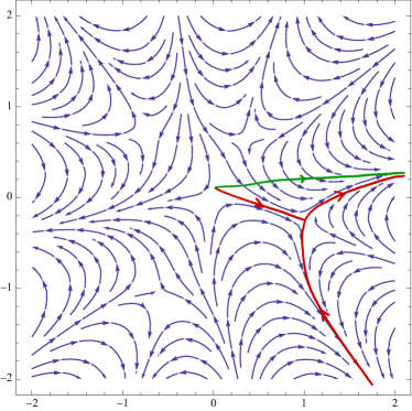
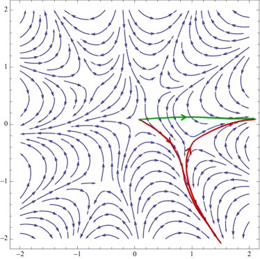
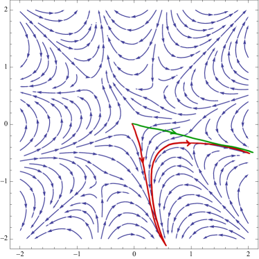
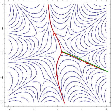
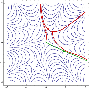
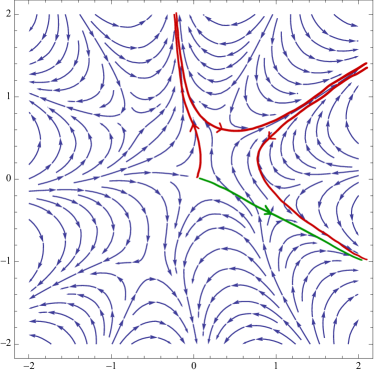
Figure 11.1. In this figure we represent the downward flow (11.63) and the mutations of Lefschetz thimbles for $|z|=10^{5}$, and $|\arg z-\arg\overline{f(\beta_{+})}|<\pi$ for the pair $(u_{1},u_{2})=(2,3e^{\frac{4\pi i}{3}})$. Lefschetz thimbles are in red. The path of integration in equation (11.61) is drawn in green. Continues in the next page.

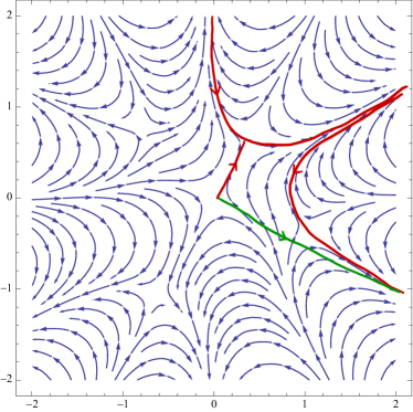
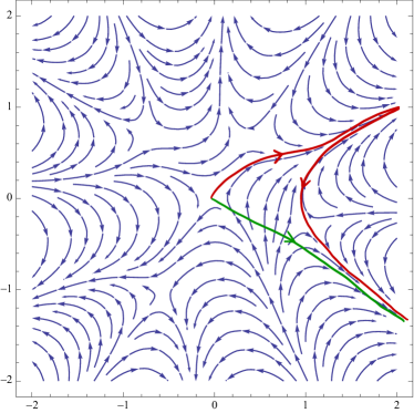
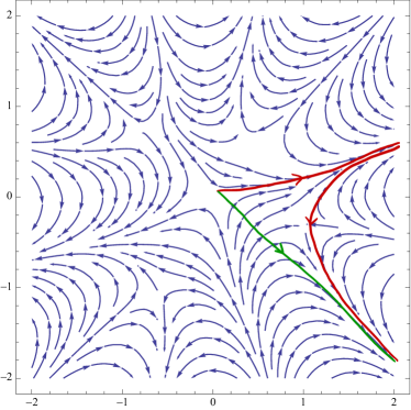
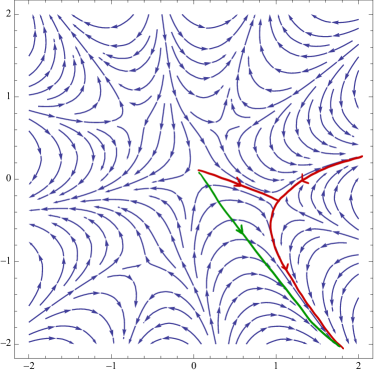
Figure 11.2. Notice that, for a certain range of values of $\arg z$, there is also a contribution in the asymptotic expansion coming from a third critical point. Such a term is negligible, since it is dominated by the exponential term from the critical point $\beta_{+}$.

Proposition 11.20.

Let now $\Phi_{1},\Phi_{2}$ be two functions with asymptotic expansions

$$\Phi_{1}(z)\sim z^{D_{1}}\exp(zu_{1}),\quad\Phi_{2}(z)\sim z^{D_{2}}\exp(zu_{2}),$$ (11.65)

for $|z|\to\infty$ in the sectors

$$A_{1}<\arg z<B_{1},\quad A_{2}<\arg z<B_{2},$$ (11.66)

respectively. We have that

$$\mathscr{L}_{(1,2;\frac{1}{2},\frac{1}{3})}[\Phi_{1},\Phi_{2};z]\sim Cz^{\frac{1}{2}+D_{1}+D_{2}}\exp{z(-\beta_{+}^{6}+u_{1}\beta_{+}^{3}+u_{2}\beta_{+}^{2})},$$

where

$$C:=6\beta_{+}^{5+2D_{1}+3D_{2}}\left(\frac{2\pi}{9u_{1}\beta_{+}+8u_{2}}\right)^{\frac{1}{2}},$$

for $|z|\to\infty$ in the sector $A^{\prime}<\arg z<B^{\prime}$, where

$$A^{\prime} :=\max\left\{A_{1}-3\arg\beta_{+},\ A_{2}-2\arg\beta_{+},\ \arg\overline{f(\beta_{+})}-\pi\right\},$$ (11.67)

$$B^{\prime} :=\min\left\{B_{1}-3\arg\beta_{+},\ B_{2}-2\arg\beta_{+},\ \arg\overline{f(\beta_{+})}+\pi\right\}.$$ (11.68)

Proof.

The statement follows by application of the steepest descent path method and Lemma 11.18. Notice that the sector $A^{\prime}<\arg z<B^{\prime}$ is chosen so that the critical point of the logarithm of the integrand lies in the region (11.66) of validity of the asymptotic expansions (11.65). ∎

$$\begin{array}[]{|c|c|c|c|}\hline\cr u_{1}&u_{2}&A^{\prime}&B^{\prime}\\ \hline\cr\hline\cr 2&3&-\pi&\frac{\pi}{3}\\ \hline\cr 2&3e^{\frac{2\pi i}{3}}&-3.71775&0.471036\\ \hline\cr 2&3e^{\frac{4\pi i}{3}}&-1.00423&1.62336\\ \hline\cr-2&3&-\pi&\frac{\pi}{3}\\ \hline\cr-2&3e^{\frac{2\pi i}{3}}&-1.00423&-0.706554\\ \hline\cr-2&3e^{\frac{4\pi i}{3}}&-1.62336&1.00423\\ \hline\cr\end{array}$$

Table 11.2. In this table we represent the values $A^{\prime}$ and $B^{\prime}$ predicted in Proposition 11.20 for all possible values of $u_{1}$ and $u_{2}$.

11.7. Stokes basis of the $qDE$ of ${\mathbb{F}}_{1}$

Set

$$s_{ij}:=s_{i}\otimes p_{j}\in\mathcal{S}({\mathbb{P}}^{1})\otimes\mathcal{S}({\mathbb{P}}^{2}),$$ (11.69)

for $i=1,2$ and $j=1,2,3$.

Theorem 11.21.

The following linear combinations of the tensors $s_{ij}$’s define a basis of $\mathcal{H}$:

$$s_{11}-5s_{22}-6s_{23},\quad s_{12}+s_{23},\quad s_{13}-s_{22}-2s_{23},\quad s_{21}-4s_{22}-5s_{23}.$$ (11.70)

Proof.

Define the column vectors

• $\boldsymbol{g}=(g_{1},g_{2})^{T}$ and $\boldsymbol{s}=(s_{1},s_{2})^{T}$, bases of $\mathcal{S}({\mathbb{P}}^{1})$,

• $\boldsymbol{h}=(h_{1},h_{2},h_{3})^{T}$ and $\boldsymbol{p}=(p_{1},p_{2},p_{3})^{T}$, bases of $\mathcal{S}({\mathbb{P}}^{2})$, respectively.

In what follow we denote by $A\otimes B$ the Kronecker tensor product of two matrices $A$ and $B$. Hence we denote

• by $\boldsymbol{g}\otimes\boldsymbol{h}$ the basis $(g_{i}\otimes h_{j})_{i,j}$ of $\mathcal{S}({\mathbb{P}}^{1})\otimes\mathcal{S}({\mathbb{P}}^{2})$.

• by $\boldsymbol{s}\otimes\boldsymbol{p}$ the basis $(s_{i}\otimes p_{j})_{i,j}$ of $\mathcal{S}({\mathbb{P}}^{1})\otimes\mathcal{S}({\mathbb{P}}^{2})$.

We have

$$\boldsymbol{g}\otimes\boldsymbol{h}=[(M_{1}M_{2}^{-1})\otimes(N_{1}N_{2}^{-1})]\boldsymbol{s}\otimes\boldsymbol{p},$$ (11.71)

where we represent the basis $\boldsymbol{g}\otimes\boldsymbol{h}$ and $\boldsymbol{s}\otimes\boldsymbol{p}$ as column vectors. Multiply on the left both sides of (11.71) by the matrix

$$E_{1}:=\left(\begin{array}[]{cccccc}1&0&0&0&0&0\\ 0&1&0&0&0&0\\ 0&0&1&0&0&0\\ 0&\frac{1}{3}&0&\frac{1}{4}&0&0\\ 0&0&0&0&1&0\\ 0&0&0&0&0&1\\ \end{array}\right).$$

We thus obtain the relation

$$\boldsymbol{s}\otimes\boldsymbol{p}=X\begin{pmatrix}g_{1}\otimes h_{1}\\ g_{1}\otimes h_{2}\\ g_{1}\otimes h_{3}\\ \frac{1}{3}g_{1}\otimes h_{2}+\frac{1}{4}g_{2}\otimes h_{1}\\ g_{2}\otimes h_{2}\\ g_{2}\otimes h_{3}\end{pmatrix},$$ (11.72)

where $X$ is the matrix

$$X =[(M_{1}M_{2}^{-1})\otimes(N_{1}N_{2}^{-1})]^{-1}E_{1}^{-1}$$

$$=\left(\begin{array}[]{cccccc}54&36(\gamma+11i\pi)&*&*&*&*\\ -54&-36(\gamma+i\pi)&*&*&*&*\\ 54&36(\gamma+3i\pi)&*&*&*&*\\ 54&36(\gamma+9i\pi)&*&*&*&*\\ -54&-36(\gamma-i\pi)&*&*&*&*\\ 54&36(\gamma+i\pi)&*&*&*&*\\ \end{array}\right).$$

Multiply on the left each sides of (11.72) by the matrix

$$E_{2}=\left(\begin{array}[]{cccccc}1&0&0&0&-5&-6\\ 0&1&0&0&0&1\\ 0&0&1&0&-1&-2\\ 0&0&0&1&-4&-5\\ 0&0&0&0&1&1\\ 0&0&0&0&0&1\\ \end{array}\right).$$

We obtain

$$\begin{pmatrix}s_{11}-5s_{22}-6s_{23}\\ s_{12}+s_{23}\\ s_{13}-s_{22}-2s_{23}\\ s_{21}-4s_{22}-5s_{23}\\ s_{22}+s_{23}\\ s_{23}\end{pmatrix}=E_{2}X\begin{pmatrix}g_{1}\otimes h_{1}\\ g_{1}\otimes h_{2}\\ g_{1}\otimes h_{3}\\ \frac{1}{3}g_{1}\otimes h_{2}+\frac{1}{4}g_{2}\otimes h_{1}\\ g_{2}\otimes h_{2}\\ g_{2}\otimes h_{3}\end{pmatrix},$$

and we have

$$E_{2}X=\left(\begin{array}[]{cc|cccc}0&0&&&&\\ 0&0&&C_{1}&&\\ 0&0&&&&\\ 0&0&&&&\\ \hline\cr 0&72i\pi&*&*&*&*\\ 54&36(\gamma+i\pi)&*&*&*&*\\ \end{array}\right).$$ (11.73)

This proves the claim. ∎

Remark 11.22.

The matrix $C_{1}$ in equation (11.73) is

$$C_{1}=\left(\begin{array}[]{cccc}24(-3i\gamma-2\pi)\pi&-216i\pi&36\pi(-5i\gamma+9\pi)&3\pi\left(-42i\gamma^{2}+92\gamma\pi+17i\pi^{2}\right)\\ 72i\gamma\pi&216i\pi&36\pi(5i\gamma+\pi)&3\pi\left(42i\gamma^{2}+12\gamma\pi-i\pi^{2}\right)\\ -72i\gamma\pi&-216i\pi&36\pi(-5i\gamma+\pi)&3\pi\left(-42i\gamma^{2}+12\gamma\pi+i\pi^{2}\right)\\ -48\pi^{2}&0&0&-48\gamma\pi^{2}\\ \end{array}\right).$$

Corollary 11.23.

The functions

$$\varSigma_{1}:= \mathscr{P}(s_{11}-5s_{22}-6s_{23}),$$ (11.74)

$$\varSigma_{2}:= \mathscr{P}(s_{12}+s_{23}),$$ (11.75)

$$\varSigma_{3}:= \mathscr{P}(s_{13}-s_{22}-2s_{23}),$$ (11.76)

$$\varSigma_{4}:= \mathscr{P}(s_{21}-4s_{22}-5s_{23})$$ (11.77)

define a basis of solutions of the $qDE$ of ${\mathbb{F}}_{1}$.∎

Proposition 11.24.

The Stokes basis $\Xi_{R}$ of $\mathcal{H}^{\rm od}_{0}$ on the sector $\Pi_{R}(\varepsilon)$ can be reconstructed, using formulae (11.6),(11.7),(11.8),(11.9), from a basis $\boldsymbol{\varSigma_{\lambda}}$ of solutions of the $qDE$ of ${\mathbb{F}}_{1}$ of the form

$$\lambda_{1}\varSigma_{2},\quad\lambda_{2}\varSigma_{3}+\lambda_{3}\varSigma_{2},\quad\lambda_{4}\varSigma_{4}+\lambda_{5}\varSigma_{3}+\lambda_{6}\varSigma_{2},\quad\lambda_{7}\varSigma_{1}+\lambda_{8}\varSigma_{4}+\lambda_{9}\varSigma_{3}+\lambda_{10}\varSigma_{2},$$

for a suitable choice of the coefficients $\lambda_{j}\in{\mathbb{C}}$, with $j=1,\dots,10$.

Proof.

The canonical coordinates $x_{1},x_{2},x_{3},x_{4}$ are in lexicographical order w.r.t. a line of slope $\varepsilon>0$ sufficiently small. The functions above have the expected expnential growth $\exp(x_{i}z)$ in the sector $\Pi_{R}(\varepsilon)$ defined by an oriented line of slope $\varepsilon$. This follows from the data in Tables 11.1 and 11.2, and from the configuration of the Stokes rays $R_{ij}:=\{-r\sqrt{-1}(\overline{x_{i}}-\overline{x_{j}})\colon r\in{\mathbb{R}}_{+}\}$: these are given by

$$R_{12} =\{\arg z=\pi\}, R_{13} =\{\arg z=2.36573\},$$

$$R_{14} =\{\arg z=1.88197\}, R_{23} =\{\arg z=0.775863\},$$

$$R_{24} =\{\arg z=1.25962\}, R_{34} =\left\{\arg z=\frac{\pi}{2}\right\},$$

see Figure 11.3. ∎

Figure 11.3. From the left to the right: Stokes rays corresponding to the origin of the quantum cohomology of ${\mathbb{P}}^{1}$, ${\mathbb{P}}^{2}$, and ${\mathbb{F}}_{1}$ respectively.

Remark 11.25.

Notice that, according to Proposition 11.20, the function $\varSigma_{3}$ has the expected exponential growth $\exp(zx_{2})$ in the sector in which this is minimal w.r.t. the dominance relation, i.e. in which it is dominated by any other exponential $\exp(zx_{1}),\exp(zx_{3}),\exp(zx_{4})$. Hence, we expect that $\lambda_{3}=0$.

11.8. Computation of the central connection and Stokes matrices

Denote by $\mathcal{H}^{\prime\prime}_{0}$ the system of differential equations $\mathcal{H}^{\rm od}_{0}$ specialized at $0\in QH^{\bullet}({\mathbb{F}}_{1})$. Consider the fundamental system of solutions of $\mathcal{H}^{\prime\prime}_{0}$

$$\Xi_{\Upsilon}(z):=\begin{pmatrix}z\Upsilon_{1}(z)&z\Upsilon_{1}(z)&z\Upsilon_{1}(z)&z\Upsilon_{1}(z)\\ \vdots&\vdots&\vdots&\vdots\end{pmatrix},$$ (11.78)

reconstructed from the basis $(\Upsilon_{1},\Upsilon_{2},\Upsilon_{3},\Upsilon_{4})$ of the $qDE$ of ${\mathbb{F}}_{1}$ (see Corollary 11.15) by formulae (11.6), (11.7), (11.8), (11.9).

Proposition 11.26.

We have

$$\Xi_{\Upsilon}(z)=\Xi_{\rm top}(z)\cdot C_{0},$$ (11.79)

where

$$C_{0}:=\begin{pmatrix}\frac{1}{18}&0&0&0\\ -\frac{\gamma}{18}&\frac{1}{2}&0&0\\ -\frac{\gamma}{18}&-\frac{1}{2}&\frac{1}{3}&0\\ \frac{6\gamma^{2}+\pi^{2}}{72}&-\frac{\gamma}{2}&-\frac{\gamma}{3}&1\end{pmatrix}.$$ (11.80)

Proof.

From Lemmata 11.9 and 11.12, we can compute the asymptotic expansions of $\Upsilon_{i}(z)$ for $z\to 0$. We have

$$\Upsilon_{1}(z)= \frac{1}{72}\left(16\log^{2}(z)-20\gamma\log(z)+6\gamma^{2}+\pi^{2}\right)+\frac{1}{18}z(\log(z)-\gamma-2)$$

$$+\frac{1}{72}z^{2}\left(16\log^{2}(z)-20\gamma\log(z)-17\log(z)+6\gamma^{2}+\pi^{2}+13\gamma+2\right)$$

$$+\frac{z^{3}\left(432\log^{2}(z)-540\gamma\log(z)-750\log(z)+162\gamma^{2}+27\pi^{2}+426\gamma+311\right)}{1944}$$

$$+\dots,$$

$$\Upsilon_{2}(z)= \frac{1}{2}(\log(z)-\gamma)-\frac{z}{2}+\frac{1}{8}z^{2}(4\log(z)-4\gamma+5)+\frac{1}{36}z^{3}(18\log(z)-18\gamma-37)$$

$$+\frac{1}{192}z^{4}(24\log(z)-24\gamma+13)+\dots,$$

$$\Upsilon_{3}(z)= -\frac{\gamma}{3}+\frac{2\log(z)}{3}+\frac{z}{3}+\frac{1}{12}z^{2}(8\log(z)-4\gamma-9)+\frac{1}{54}z^{3}(36\log(z)-18\gamma-17)$$

$$+\frac{1}{288}z^{4}(48\log(z)-24\gamma-49)+\dots,$$

$$\Upsilon_{4}(z)= 1+z^{2}+z^{3}+\frac{z^{4}}{4}+\dots.$$

After some computations, one finds that the first terms of the asymptotic expansion of $\Xi_{\Upsilon}(z)$ for $z\to 0$:

$$\Xi_{\Upsilon}(z)=$$

$$\left(\begin{array}[]{cccc}\frac{1}{72}z\left(16\log^{2}(z)-20\gamma\log(z)+6\gamma^{2}+\pi^{2}\right)&\frac{1}{2}z(\log(z)-\gamma)&z\left(\frac{2\log(z)}{3}-\frac{\gamma}{3}\right)&z\\ \frac{\log(z)}{6}-\frac{\gamma}{9}&0&\frac{1}{3}&0\\ \frac{\log(z)}{9}+\frac{1}{18}z(\log(z)-\gamma-1)-\frac{\gamma}{18}&\frac{1}{2}-\frac{z}{2}&\frac{z}{3}&0\\ \frac{1}{18}z(2\log(z)-\gamma-1)+\frac{1}{18z}&\frac{z}{2}&0&0\\ \end{array}\right)$$

$$\quad\quad+\text{h.o.t.}.$$

The leading term of the asymptotic expansion of $\Xi_{\rm top}(z)$ for $z\to 0$ is

$$\Xi_{\rm top}(z) =\eta z^{\mu}z^{R}+\text{h.o.t.}$$

$$=\left(\begin{array}[]{cccc}4z\log^{2}(z)&3z\log(z)&2z\log(z)&z\\ 3\log(z)&1&1&0\\ 2\log(z)&1&0&0\\ \frac{1}{z}&0&0&0\\ \end{array}\right)+\text{h.o.t.},$$

where $\mu={\rm diag}(-1,0,0,1)$ and $R$ is the operator of $\cup$-multiplication by $c_{1}({\mathbb{F}}_{1})$ on $H^{\bullet}({\mathbb{F}}_{1},{\mathbb{C}})$, that is

$$R=\left(\begin{array}[]{cccc}0&0&0&0\\ 2&0&0&0\\ 1&0&0&0\\ 0&3&2&0\\ \end{array}\right).$$ (11.81)

By comparison of the leading terms of the asymptotic expansions of $\Xi_{\Upsilon}$ and $\Xi_{\rm top}$, one obtains the matrix $C_{0}$ in formula (11.80). ∎

Theorem 11.27.

The central connection and Stokes matrices at $0\in QH^{\bullet}({\mathbb{F}}_{1})$, computed w.r.t. an admissible oriented line of slope $\varepsilon>0$ sufficiently small, equal

$$C=\left(\begin{array}[]{cccc}\frac{1}{2\pi}&-\frac{1}{2\pi}&\frac{1}{2\pi}&-\frac{1}{2\pi}\\ \frac{\gamma}{\pi}&-\frac{\gamma}{\pi}&i+\frac{\gamma}{\pi}&-i-\frac{\gamma}{\pi}\\ \frac{1}{2}\left(-i+\frac{\gamma}{\pi}\right)&-\frac{\gamma+i\pi}{2\pi}&\frac{1}{2}\left(-i+\frac{\gamma}{\pi}\right)&-\frac{\gamma+i\pi}{2\pi}\\ \gamma\left(-i+\frac{2\gamma}{\pi}\right)&\gamma\left(-i-\frac{2\gamma}{\pi}\right)&\frac{2\gamma(\gamma+i\pi)}{\pi}&-\frac{2(\gamma+i\pi)^{2}}{\pi}\\ \end{array}\right),$$ (11.82)

$$S=\left(\begin{array}[]{cccc}1&2&-1&-3\\ 0&1&1&-1\\ 0&0&1&2\\ 0&0&0&1\\ \end{array}\right).$$ (11.83)

Proof.

Denote

• by $\Xi_{\boldsymbol{\lambda}}$ the fundamental system of solutions of $\mathcal{H}^{\prime\prime}_{0}$ constructed from the basis $\boldsymbol{\varSigma_{\lambda}}$ of Proposition 11.24,

• by $\Xi_{\varSigma}$ the fundamental system of solutions of $\mathcal{H}^{\prime\prime}_{0}$ constructed from the basis $\boldsymbol{\varSigma}$ of Corollary 11.23.

We have

$$\Xi_{\boldsymbol{\lambda}}= \Xi_{\varSigma}\cdot\left(\begin{array}[]{cccc}0&0&0&\lambda_{7}\\ \lambda_{1}&\lambda_{3}&\lambda_{6}&\lambda_{10}\\ 0&\lambda_{2}&\lambda_{5}&\lambda_{9}\\ 0&0&\lambda_{4}&\lambda_{8}\\ \end{array}\right)=\Xi_{\Upsilon}\Pi^{T}C_{1}^{T}\left(\begin{array}[]{cccc}0&0&0&\lambda_{7}\\ \lambda_{1}&\lambda_{3}&\lambda_{6}&\lambda_{10}\\ 0&\lambda_{2}&\lambda_{5}&\lambda_{9}\\ 0&0&\lambda_{4}&\lambda_{8}\\ \end{array}\right),$$

where $C_{1}$ is as in Remark 11.22 and

$$\Pi:=\left(\begin{array}[]{cccc}0&1&0&0\\ 1&0&0&0\\ 0&0&1&0\\ 0&0&0&1\\ \end{array}\right).$$

Thus, we obtain

$$\Xi_{\boldsymbol{\lambda}}=\Xi_{\rm top}C_{\boldsymbol{\lambda}},\quad C_{\boldsymbol{\lambda}}:=C_{0}\Pi^{T}C_{1}^{T}\left(\begin{array}[]{cccc}0&0&0&\lambda_{7}\\ \lambda_{1}&\lambda_{3}&\lambda_{6}&\lambda_{10}\\ 0&\lambda_{2}&\lambda_{5}&\lambda_{9}\\ 0&0&\lambda_{4}&\lambda_{8}\\ \end{array}\right),$$

where $C_{0}$ is given by (11.80). In order to determine the values of $\boldsymbol{\lambda}$ for which $\Xi_{\boldsymbol{\lambda}}$ is the Stokes basis, let us compute the product

$$C_{\boldsymbol{\lambda}}^{T}\eta e^{\pi i\mu}e^{\pi iR}C_{\boldsymbol{\lambda}}.$$ (11.84)

If $\Xi_{\boldsymbol{\lambda}}$ is the Stokes basis, then the matrix above is the inverse of the Stokes matrix $S$, by equation (4.18): in particular, it is an upper triangular matrix with 1’s along the main diagonal. An explicit computation gives the following result: the columns of (11.84) are

$$\left(\begin{array}[]{c}-576\pi^{4}\lambda_{1}^{2}\\ -576\pi^{4}\lambda_{1}\lambda_{3}\\ -576\pi^{4}\lambda_{1}\lambda_{6}\\ -576\pi^{4}\lambda_{1}\left(3\lambda_{7}+\lambda_{10}\right)\\ \end{array}\right),$$ (11.85)

$$\left(\begin{array}[]{c}576\pi^{4}\lambda_{1}\left(2\lambda_{2}-\lambda_{3}\right)\\ -576\pi^{4}\left(\lambda_{2}-\lambda_{3}\right){}^{2}\\ -576\pi^{4}\left(\lambda_{3}\lambda_{6}+\lambda_{2}\left(\lambda_{4}+\lambda_{5}-2\lambda_{6}\right)\right)\\ 576\pi^{4}\left(\lambda_{2}\left(\lambda_{7}-\lambda_{8}-\lambda_{9}+2\lambda_{10}\right)-\lambda_{3}\left(3\lambda_{7}+\lambda_{10}\right)\right)\\ \end{array}\right),$$ (11.86)

$$\left(\begin{array}[]{c}-576\pi^{4}\lambda_{1}\left(\lambda_{4}-2\lambda_{5}+\lambda_{6}\right)\\ -576\pi^{4}\left(\lambda_{2}\lambda_{5}+\lambda_{3}\left(\lambda_{4}-2\lambda_{5}+\lambda_{6}\right)\right)\\ -576\pi^{4}\left(\lambda_{4}^{2}+\left(\lambda_{5}+\lambda_{6}\right)\lambda_{4}+\left(\lambda_{5}-\lambda_{6}\right){}^{2}\right)\\ -576\pi^{4}\left(\lambda_{6}\left(3\lambda_{7}+\lambda_{10}\right)+\lambda_{4}\left(5\lambda_{7}+\lambda_{8}+\lambda_{10}\right)+\lambda_{5}\left(-\lambda_{7}+\lambda_{8}+\lambda_{9}-2\lambda_{10}\right)\right)\\ \end{array}\right),$$ (11.87)

$$\left(\begin{array}[]{c}576\pi^{4}\lambda_{1}\left(6\lambda_{7}-\lambda_{8}+2\lambda_{9}-\lambda_{10}\right)\\ -576\pi^{4}\left(\lambda_{2}\left(6\lambda_{7}+\lambda_{9}\right)+\lambda_{3}\left(-6\lambda_{7}+\lambda_{8}-2\lambda_{9}+\lambda_{10}\right)\right)\\ -576\pi^{4}\left(\lambda_{5}\left(6\lambda_{7}+\lambda_{9}\right)+\lambda_{4}\left(6\lambda_{7}+\lambda_{8}+\lambda_{9}\right)+\lambda_{6}\left(-6\lambda_{7}+\lambda_{8}-2\lambda_{9}+\lambda_{10}\right)\right)\\ -576\pi^{4}\left(13\lambda_{7}^{2}+\left(11\lambda_{8}+5\lambda_{9}-3\lambda_{10}\right)\lambda_{7}+\lambda_{8}^{2}+\left(\lambda_{9}-\lambda_{10}\right){}^{2}+\lambda_{8}\left(\lambda_{9}+\lambda_{10}\right)\right)\\ \end{array}\right).$$ (11.88)

The matrix (11.84) is upper triangular with 1’s along the diagonal if and only if

$$\lambda_{1}^{2}= -\frac{1}{576\pi^{4}}, \lambda_{2}^{2}= -\frac{1}{576\pi^{4}},$$ (11.89)

$$\lambda_{3}= \ 0, \lambda_{4}^{2}= -\frac{1}{576\pi^{4}},$$ (11.90)

$$\lambda_{5}= -\lambda_{4}, \lambda_{6}= \ 0,$$ (11.91)

$$\lambda_{7}^{2}= -\frac{1}{576\pi^{4}}, \lambda_{8}= -2\lambda_{7},$$ (11.92)

$$\lambda_{9}= -3\lambda_{7}, \lambda_{10}= -3\lambda_{7}.$$ (11.93)

For the choice $\lambda_{1}=\lambda_{2}=\lambda_{4}=\lambda_{7}=-\frac{i}{24\pi^{2}}$, we obtain the central connection and Stokes matrices (11.82) and (11.83). ∎

Theorem 11.28.

The central connection matrix of $QH^{\bullet}({\mathbb{F}}_{2k+1})$, computed w.r.t. an oriented line of slope $\varepsilon>0$ sufficiently small, and a suitable choice of the branch of the $\Psi$-matrix, equals

$$C_{k}=\left(\begin{array}[]{cccc}\frac{1}{2\pi}&-\frac{1}{2\pi}&\frac{1}{2\pi}&-\frac{1}{2\pi}\\ \frac{\gamma}{\pi}&-\frac{\gamma}{\pi}&i+\frac{\gamma}{\pi}&-i-\frac{\gamma}{\pi}\\ \frac{\gamma-2\gamma k-i\pi}{2\pi}&-\frac{\gamma-2\gamma k+i\pi}{2\pi}&\frac{-2\gamma k-i(2\pi k+\pi)+\gamma}{2\pi}&\frac{(2k-1)(\gamma+i\pi)}{2\pi}\\ \gamma\left(-i+\frac{2\gamma}{\pi}\right)&\gamma\left(-i-\frac{2\gamma}{\pi}\right)&\frac{2\gamma(\gamma+i\pi)}{\pi}&-\frac{2(\gamma+i\pi)^{2}}{\pi}\\ \end{array}\right).$$ (11.94)

This is the matrix associated with the morphism

$$\textnormal{\textcyr{D}}^{-}_{\mathbb{F}_{2k+1}}\colon K_{0}(\mathbb{F}_{2k+1})_{\mathbb{C}}\to H^{\bullet}(\mathbb{F}_{2k+1},\mathbb{C})\colon[\mathscr{F}]\mapsto\frac{1}{2\pi}\widehat{\Gamma}^{-}_{\mathbb{F}_{2k+1}}\cup e^{-\pi ic_{1}(\mathbb{F}_{2k+1})}\cup{\rm Ch}(\mathscr{F}),$$

w.r.t. an exceptional basis $\mathfrak{E}:=(E_{i})_{i=1}^{4}$ of $K_{0}(\mathbb{F}_{2k+1})_{\mathbb{C}}$ and the basis $(T_{i,2k+1})_{i=0}^{3}$ of $H^{\bullet}(\mathbb{F}_{2k+1},\mathbb{C})$. The exceptional basis $\mathfrak{E}$ mutates to the exceptional basis

$$\left([\mathcal{O}],[\mathcal{O}(\Sigma_{2}^{2k+1})],[\mathcal{O}(\Sigma_{4}^{2k+1})],[\mathcal{O}(\Sigma_{2}^{2k+1}+\Sigma_{4}^{2k+1})]\right),$$ (11.95)

by application of the following natural transformations:

1. action of the braid $\beta_{3}\beta_{2}\beta_{1}\beta_{3}\beta_{2}$;

2. action of the element $\tilde{J}_{k}\in({\mathbb{Z}}/2{\mathbb{Z}})^{4}$

   $$(-1,-1,(-1)^{p},(-1)^{p+1}),\quad\text{if }k=2p,$$

   $$(-1,-1,(-1)^{p+1},(-1)^{p+1}),\quad\text{if }k=2p+1;$$

3. action of the element $\beta_{3}^{k}$.

Proof.

The matrix associated to $\textnormal{\textcyr{D}}^{-}_{\mathbb{F}_{2k+1}}$ w.r.t. the basis (11.95) is ∎

$$E_{k}:=\left(\begin{array}[]{cccc}\frac{1}{2\pi}&\frac{1}{2\pi}&\frac{1}{2\pi}&\frac{1}{2\pi}\\ -i+\frac{\gamma}{\pi}&-i+\frac{\gamma}{\pi}&\frac{\gamma}{\pi}&\frac{\gamma}{\pi}\\ \frac{(1-2k)(\gamma-i\pi)}{2\pi}&\frac{-2\gamma k+i(2\pi k+\pi)+\gamma}{2\pi}&\frac{(1-2k)(\gamma-i\pi)}{2\pi}&\frac{-2\gamma k+i(2\pi k+\pi)+\gamma}{2\pi}\\ \frac{2(\gamma-i\pi)^{2}}{\pi}&\frac{2\gamma(\gamma-i\pi)}{\pi}&\gamma\left(-i+2ik+\frac{2\gamma}{\pi}\right)&\gamma\left(i+2ik+\frac{2\gamma}{\pi}\right)\\ \end{array}\right).$$

Set $C_{k}^{\prime}:=C_{k}^{\beta_{3}\beta_{2}\beta_{1}\beta_{3}\beta_{2}}$. We have

$$(C^{\prime}_{k})^{-1}E_{k}=\left(\begin{array}[]{cccc}-1&0&0&0\\ 0&-1&0&0\\ 0&0&1-k&-k\\ 0&0&-k&-k-1\\ \end{array}\right).$$

It is easy to see that this is the matrix representing the action of the element $(\tilde{J}_{k},\beta_{3}^{k})\in({\mathbb{Z}}/2{\mathbb{Z}})^{4}\rtimes\mathcal{B}_{4}$: the argument is the same as in Step 3 of the proof of Theorem 10.5. ∎

Appendix A Proof of Theorem 5.2

We need some preliminary results.

Lemma A.1.

For $n\geqslant 0$, and $\delta\in H^{2}(X,{\mathbb{C}})$, we have

$$\mathopen{\hbox{\set@color${\langle}$}\kern-1.94444pt\leavevmode\hbox{\set@color${\langle}$}}\tau_{n}T_{\alpha},1\mathclose{\hbox{\set@color${\rangle}$}\kern-1.94444pt\leavevmode\hbox{\set@color${\rangle}$}}_{0}(\delta)=\frac{1}{(n+1)!}\left(\int_{X}T_{\alpha}\cup\delta^{n+1}\right)+\sum_{\beta\neq 0}\sum_{\nu\geqslant 0}\frac{{\bf Q}^{\beta}e^{\int_{\beta}\delta}}{\nu!}\langle\tau_{n-\nu}T_{\alpha}\cup\delta^{\nu},1\rangle^{X}_{0,2,\beta}.$$

Proof.

We have

$$\mathopen{\hbox{\set@color${\langle}$}\kern-1.94444pt\leavevmode\hbox{\set@color${\langle}$}}\tau_{n}T_{\alpha},1\mathclose{\hbox{\set@color${\rangle}$}\kern-1.94444pt\leavevmode\hbox{\set@color${\rangle}$}}_{0}(\delta) =\left.\frac{\partial}{\partial t^{\alpha,n}}\frac{\partial}{\partial t^{0,0}}\mathcal{F}^{X}_{0}\right|_{\delta}=\sum_{k=0}^{\infty}\sum_{\beta}\frac{{\bf Q}^{\beta}}{k!}\langle\tau_{n}T_{\alpha},1,\delta\,\dots,\delta\rangle^{X}_{0,k+2,\beta}.$$

We have two cases:

• if $\beta\neq 0$, then for $k\geqslant 0$ we have

  $$\langle\tau_{n}T_{\alpha},1,\delta\,\dots,\delta\rangle^{X}_{0,k+2,\beta}=\sum_{\mu+\nu=k}\frac{k!}{\mu!\nu!}\left(\int_{\beta}\delta\right)^{\mu}\langle\tau_{n-\nu}T_{\alpha}\cup\delta^{\nu},1\rangle^{X}_{0,2,\beta},$$

  by the Divisor Axiom of Gromov-Witten invariants. Here any invariant with $\tau_{-r}$ with $r>0$ is vanishing.

• If $\beta=0$, then for $k>0$ by Divisor Axiom we have

  $$\langle\tau_{n}T_{\alpha},1,\delta\,\dots,\delta\rangle^{X}_{0,k+2,0}=\langle\tau_{n-k+1}T_{\alpha}\cup\delta^{k},1,\delta\rangle_{0,3,0}=\left(\int_{X}T_{\alpha}\cup\delta^{k}\right)\delta_{k,n+1}.$$

So, we have

$$\mathopen{\hbox{\set@color${\langle}$}\kern-1.94444pt\leavevmode\hbox{\set@color${\langle}$}}\tau_{n}T_{\alpha},1\mathclose{\hbox{\set@color${\rangle}$}\kern-1.94444pt\leavevmode\hbox{\set@color${\rangle}$}}_{0}(\delta)= \frac{1}{(n+1)!}\left(\int_{X}T_{\alpha}\cup\delta^{n+1}\right)$$

$$+\sum_{\beta\neq 0}\sum_{k\geqslant 0}\frac{{\bf Q^{\beta}}}{k!}\sum_{\mu+\nu=k}\frac{k!}{\mu!\nu!}\left(\int_{\beta}\delta\right)^{\mu}\langle\tau_{n-\nu}T_{\alpha}\cup\delta^{\nu},1\rangle^{X}_{0,2,\beta}$$

$$= \frac{1}{(n+1)!}\left(\int_{X}T_{\alpha}\cup\delta^{n+1}\right)+\sum_{\beta\neq 0}\sum_{\nu\geqslant 0}\frac{{\bf Q}^{\beta}e^{\int_{\beta}\delta}}{\nu!}\langle\tau_{n-\nu}T_{\alpha}\cup\delta^{\nu},1\rangle^{X}_{0,2,\beta}.\quad\quad\qed$$

Lemma A.2.

Let $\delta\in H^{2}(X,{\mathbb{C}})$. We have

$$J_{X}(\delta)=e^{\frac{\delta}{\hbar}}+\sum_{\beta\neq 0}\sum_{n=0}^{\infty}\sum_{k+p=n}\hbar^{-(n+1)}\frac{{\bf Q}^{\beta}e^{\int_{\beta}\delta}}{p!}\langle\tau_{k}T_{\alpha}\cup\delta^{p},1\rangle^{X}_{0,2,\beta}T^{\alpha}.$$

Proof.

By Lemma A.1, we have

$$J_{X}(\delta)= 1+\sum_{n=0}^{\infty}\frac{\hbar^{-(n+1)}}{(n+1)!}\left(\int_{X}T_{\alpha}\cup\delta^{n+1}\right)T^{\alpha}$$

$$+\sum_{\beta\neq 0}\sum_{n=0}^{\infty}\sum_{k+p=n}\hbar^{-(n+1)}\frac{{\bf Q}^{\beta}e^{\int_{\beta}\delta}}{p!}\langle\tau_{k}T_{\alpha}\cup\delta^{p},1\rangle^{X}_{0,2,\beta}T^{\alpha}$$

$$= e^{\frac{\delta}{\hbar}}+\sum_{\beta\neq 0}\sum_{n=0}^{\infty}\sum_{k+p=n}\hbar^{-(n+1)}\frac{{\bf Q}^{\beta}e^{\int_{\beta}\delta}}{p!}\langle\tau_{k}T_{\alpha}\cup\delta^{p},1\rangle^{X}_{0,2,\beta}T^{\alpha}.\qed$$

Lemma A.3.

For $\delta\in H^{2}(X,{\mathbb{C}})$, we have

$$Z_{\rm top}(\delta,z)T_{\alpha}=e^{z\delta}\cup z^{\mu}z^{c_{1}(X)}T_{\alpha}+\sum_{\beta\neq 0}\sum_{\lambda}e^{\int_{\beta}\delta}\bigg{\langle}\frac{ze^{z\delta}}{1-z\psi}\cup z^{\mu}z^{c_{1}(X)}T_{\alpha},T_{\lambda}\bigg{\rangle}^{X}_{0,2,\beta}T^{\lambda}.$$ (A.1)

Proof.

For $\boldsymbol{\tau}\in H^{\bullet}(X,{\mathbb{C}})$, we have

$$\Theta(\boldsymbol{\tau},z)T_{\alpha}= \Theta(\boldsymbol{\tau},z)_{\alpha}^{\beta}T_{\beta}=\left.\frac{\partial\theta_{\alpha}}{\partial t^{\lambda}}\right|_{(\boldsymbol{\tau},z)}T^{\lambda}$$

$$= \sum_{p=0}^{\infty}z^{p}\mathopen{\hbox{\set@color${\langle}$}\kern-1.94444pt\leavevmode\hbox{\set@color${\langle}$}}\tau_{p}T_{\alpha},1,T_{\lambda}\mathclose{\hbox{\set@color${\rangle}$}\kern-1.94444pt\leavevmode\hbox{\set@color${\rangle}$}}_{0}(\boldsymbol{\tau})|_{\bf Q=1}T^{\lambda}$$

$$= \sum_{p=0}^{\infty}\sum_{k=0}^{\infty}\sum_{\beta}\frac{z^{p}}{k!}\langle\tau_{p}T_{\alpha},1,T_{\lambda},\boldsymbol{\tau},\dots,\boldsymbol{\tau}\rangle^{X}_{0,3+k,\beta}T^{\lambda}.$$

Consider the contribution coming from $(k,\beta)=(0,0)$: by the Mapping to point Axiom of Gromov-Witten invariants, we have

$$\sum_{p=0}^{\infty}{z^{p}}\langle\tau_{p}T_{\alpha},1,T_{\lambda},\rangle^{X}_{0,3,0}T^{\lambda}=\sum_{p=0}^{\infty}z^{p}\left(\int_{X}T_{\alpha}\cup T_{\lambda}\right)\delta_{0,p}T^{\lambda}=T_{\alpha}.$$

By the Fundamental class Axiom, instead, the contribution from $(k,\beta)\neq(0,0)$ can be re-written as

$$\sum_{p=0}^{\infty}\sum_{k=1}^{\infty}\sum_{\beta\neq 0}\frac{z^{p}}{k!}\langle\tau_{p-1}T_{\alpha},T_{\lambda},\boldsymbol{\tau},\dots,\boldsymbol{\tau}\rangle^{X}_{0,2+k,\beta}T^{\lambda}.$$

Thus, we have recovered the formula

$$\Theta(\boldsymbol{\tau},z)={\rm Id}+\sum_{p=0}^{\infty}z^{p+1}\mathopen{\hbox{\set@color${\langle}$}\kern-1.94444pt\leavevmode\hbox{\set@color${\langle}$}}\tau_{p}(-),T_{\lambda}\mathclose{\hbox{\set@color${\rangle}$}\kern-1.94444pt\leavevmode\hbox{\set@color${\rangle}$}}_{0}(\boldsymbol{\tau})|_{\bf Q=1}T^{\lambda},$$

which was used in [CDG20, Proposition 7.1] to define $\Theta$. At this point the proof is known, and can be found in [CK99, Proposition 10.2.3]: the parameter $\hbar$ of loc. cit. has to be replaced by our $z$, and pre-composition with $z^{\mu}z^{c_{1}(X)}$ has to be taken into account in order to obtain formula (A.1). ∎

We are now ready for the proof of Theorem 5.2.

Proof of Theorem 5.2.

Let us compute the entries of the first row of the matrix

$$\eta\Theta(\delta,z)z^{\mu}z^{c_{1}(X)}.$$

By Lemma A.3, we have

$$\left[\eta\Theta(\delta,z)z^{\mu}z^{c_{1}(X)}\right]^{1}_{\alpha}=\eta\left(1,\Theta(\delta,z)z^{\mu}z^{c_{1}(X)}T_{\alpha}\right)$$

$$=\eta\left(1,e^{z\delta}\cup z^{\mu}z^{c_{1}(X)}T_{\alpha}+\sum_{\beta\neq 0}\sum_{\lambda}e^{\int_{\beta}\delta}\bigg{\langle}\frac{ze^{z\delta}}{1-z\psi}\cup z^{\mu}z^{c_{1}(X)}T_{\alpha},T_{\lambda}\bigg{\rangle}^{X}_{0,2,\beta}T^{\lambda}\right)$$

$$=\eta(1,e^{z\delta}\cup z^{\mu}z^{c_{1}(X)}T_{\alpha})$$

$$+\eta\left(1,\sum_{\beta\neq 0}\sum_{\lambda}e^{\int_{\beta}\delta}\bigg{\langle}\frac{ze^{z\delta}}{1-z\psi}\cup z^{\mu}z^{c_{1}(X)}T_{\alpha},T_{\lambda}\bigg{\rangle}^{X}_{0,2,\beta}T^{\lambda}\right).$$

Using the identity of endomorphisms of $H^{\bullet}(X,\mathbb{C})$

$$z^{-\mu}\circ(h^{k}\cup)\circ z^{\mu}=z^{-k}(h^{k}\cup),\quad h\in H^{2}(X,\mathbb{C}),\quad k\in\mathbb{N},$$

and the $\eta$-skew-symmetry of $\mu$, we can rewrite the first summand as

$$\eta(1,e^{z\delta}\cup z^{\mu}z^{c_{1}(X)}T_{\alpha}) =\eta(1,z^{\mu}e^{\delta}z^{c_{1}(X)}T_{\alpha})$$

$$=\eta(z^{-\mu}(1),e^{\delta}z^{c_{1}(X)}T_{\alpha})$$

$$=z^{\frac{\dim_{\mathbb{C}}X}{2}}\int_{X}e^{\delta}z^{c_{1}(X)}T_{\alpha}.$$

For the second summand, notice that

1. the only nonzero contribution comes from $\lambda=0$,

2. for any $\varphi\in H^{\bullet}(X,\mathbb{C})$ we have that

   $$\frac{ze^{z\delta}}{1-z\psi}\cup\varphi=\sum_{n=0}^{\infty}\sum_{k=0}^{n}\frac{z^{n+1}}{(n-k)!}\psi^{k}\delta^{n-k}\varphi,$$

3. and that

   $$z^{\mu}z^{c_{1}(X)}T_{\alpha}=\sum_{\ell=0}^{\infty}\frac{(\log z)^{\ell}}{\ell!}z^{\frac{2\ell+\deg T_{\alpha}-\dim X}{2}}c_{1}(X)^{\ell}T_{\alpha}.$$

4. the Gromov-Witten invariant

   $$\langle\tau_{k}\delta^{n-k}c_{1}(X)^{\ell}T_{\alpha},1\rangle^{X}_{0,2,\beta}$$

   is nonzero if and only if

   $$2k+2(n-k)+2\ell+\deg T_{\alpha}=2\dim_{\mathbb{C}}X+2\int_{\beta}c_{1}(X)-2.$$

So, we obtain that

$$\bigg{\langle}\frac{ze^{z\delta}}{1-z\psi}\cup z^{\mu}z^{c_{1}(X)}T_{\alpha},1\bigg{\rangle}^{X}_{0,2,\beta}$$

$$=\sum_{n=0}^{\infty}\sum_{k=0}^{n}\sum_{\ell=0}^{\infty}\frac{(\log z)^{\ell}}{\ell!(n-k)!}z^{n+1+\frac{2\ell+\deg T_{\alpha}-\dim X}{2}}\langle\tau_{k}\delta^{n-k}c_{1}(X)^{\ell}T_{\alpha},1\rangle^{X}_{0,2,\beta}$$

$$=z^{\frac{\dim X}{2}}z^{\int_{\beta}c_{1}(X)}\sum_{h=0}^{\infty}\sum_{m+\ell+k=h}\frac{(\log z)^{\ell}}{\ell!m!}\langle\tau_{k}\delta^{m}c_{1}(X)^{\ell}T_{\alpha},1\rangle^{X}_{0,2,\beta}$$

$$=z^{\frac{\dim X}{2}}z^{\int_{\beta}c_{1}(X)}\sum_{h=0}^{\infty}\sum_{k+p=h}\frac{1}{p!}\langle\tau_{k}(\delta+\log z\cdot c_{1}(X))^{p}T_{\alpha},1\rangle^{X}_{0,2,\beta}.$$

Putting this all together, we obtain that

$$\left[\eta\Theta(\delta,z)z^{\mu}z^{c_{1}(X)}\right]^{1}_{\alpha}$$

$$=z^{\frac{\dim X}{2}}\left(\int_{X}e^{\delta}z^{c_{1}(X)}T_{\alpha}+\sum_{\beta\neq 0}e^{\int_{\beta}\delta}z^{\int_{\beta}c_{1}(X)}\sum_{h=0}^{\infty}\sum_{k+p=h}\frac{1}{p!}\langle\tau_{k}(\delta+\log z\cdot c_{1}(X))^{p}T_{\alpha},1\rangle^{X}_{0,2,\beta}\right)$$

$$=z^{\frac{\dim X}{2}}\int_{X}T_{\alpha}\cup J_{X}(\delta+\log z\cdot c_{1}(X))\Big{|}_{\begin{subarray}{c}{\bf Q}=1,\\ \hbar=1\end{subarray}}.$$

The last equality follows by Lemma A.2. This completes the proof. ∎

Appendix B Coefficients $\mathcal{A}_{j}^{(i)},\mathcal{B}_{j}^{(i)}$

The coefficients $\mathcal{A}_{j}^{(i)},\mathcal{B}_{j}^{(i)}$ are

$$\mathcal{A}_{1}^{(1)}(m,n)= -\frac{8}{9}mn^{2}A_{0,0}B_{0,0},$$

$$\mathcal{A}_{2}^{(1)}(m,n)= \ \frac{8}{9}n^{2}A_{0,0}B_{0,0},$$

$$\mathcal{A}_{3}^{(1)}(m,n)= \ \frac{8}{9}mA_{0,0}B_{0,0},$$

$$\mathcal{A}_{1}^{(2)}(m,n)= \ \frac{4}{9}n\left(4mnA_{0,0}B_{0,0}H_{m}+6mnA_{0,0}B_{0,0}H_{n}\right.$$

$$-4mnA_{0,1}B_{0,0}-3mnA_{0,0}B_{0,1}-4mnA_{0,0}B_{0,0}\psi^{(0)}(m+n+1)$$

$$\left.-4mA_{0,0}B_{0,0}-2nA_{0,0}B_{0,0}\right),$$

$$\mathcal{A}_{2}^{(2)}(m,n)= -\frac{4}{9}n\left(4nA_{0,0}B_{0,0}H_{m}+6nA_{0,0}B_{0,0}H_{n}\right.$$

$$\left.-4nA_{0,0}B_{0,0}\psi^{(0)}(m+n+1)-4nA_{0,1}B_{0,0}-3nA_{0,0}B_{0,1}-4A_{0,0}B_{0,0}\right),$$

$$\mathcal{A}_{3}^{(2)}(m,n)= -\frac{4}{9}\left(6mA_{0,0}B_{0,0}H_{n}+4mA_{0,0}B_{0,0}H_{m}\right.$$

$$\left.-4mA_{0,0}B_{0,0}\psi^{(0)}(m+n+1)-4mA_{0,1}B_{0,0}-3mA_{0,0}B_{0,1}-2A_{0,0}B_{0,0}\right),$$

$$\mathcal{A}_{1}^{(3)}(m,n)= -\frac{2}{9}\left(24mn^{2}A_{0,0}B_{0,0}H_{m}H_{n}-24mn^{2}A_{0,1}B_{0,0}H_{n}-12mn^{2}A_{0,0}B_{0,1}H_{m}\right.$$

$$-8mn^{2}A_{0,0}B_{0,0}H_{m}\psi^{(0)}(m+n+1)-18mn^{2}A_{0,0}B_{0,0}H_{n}\psi^{(0)}(m+n+1)$$

$$-16mnA_{0,0}B_{0,0}H_{m}-12mnA_{0,0}B_{0,0}H_{n}-12n^{2}A_{0,0}B_{0,0}H_{n}$$

$$+12mn^{2}A_{0,1}B_{0,1}+9mn^{2}A_{0,0}B_{n,2}+5mn^{2}A_{0,0}B_{0,0}\psi^{(0)}(m+n+1)^{2}$$

$$+4n^{2}A_{0,0}B_{0,0}\psi^{(0)}(m+n+1)+5mn^{2}A_{0,0}B_{0,0}\psi^{(1)}(m+n+1)$$

$$+8mn^{2}A_{0,1}B_{0,0}\psi^{(0)}(m+n+1)+9mn^{2}A_{0,0}B_{0,1}\psi^{(0)}(m+n+1)$$

$$+16mnA_{0,1}B_{0,0}+6mnA_{0,0}B_{0,1}+12mnA_{0,0}B_{0,0}\psi^{(0)}(m+n+1)$$

$$+2mA_{0,0}B_{0,0}+6n^{2}A_{0,0}B_{0,1}+8nA_{0,0}B_{0,0}\left.\right),$$

$$\mathcal{A}_{2}^{(3)}(m,n)= \ \frac{2}{9}\left(24n^{2}A_{0,0}B_{0,0}H_{m}H_{n}-12n^{2}A_{0,0}B_{0,1}H_{m}\right.$$

$$-8n^{2}A_{0,0}B_{0,0}H_{m}\psi^{(0)}(m+n+1)-18n^{2}A_{0,0}B_{0,0}H_{n}\psi^{(0)}(m+n+1)$$

$$-16nA_{0,0}B_{0,0}H_{m}-24n^{2}A_{0,1}B_{0,0}H_{n}-12nA_{0,0}B_{0,0}H_{n}$$

$$+5n^{2}A_{0,0}B_{0,0}\psi^{(0)}(m+n+1)^{2}+5n^{2}A_{0,0}B_{0,0}\psi^{(1)}(m+n+1)$$

$$+8n^{2}A_{0,1}B_{0,0}\psi^{(0)}(m+n+1)+9n^{2}A_{0,0}B_{0,1}\psi^{(0)}(m+n+1)$$

$$+12nA_{0,0}B_{0,0}\psi^{(0)}(m+n+1)+12n^{2}A_{0,1}B_{0,1}+9n^{2}A_{0,0}B_{n,2}$$

$$+16nA_{0,1}B_{0,0}+6nA_{0,0}B_{0,1}+2A_{0,0}B_{0,0}\left.\right),$$

$$\mathcal{A}_{3}^{(3)}(m,n)= \ \frac{2}{9}\left(24mA_{0,0}B_{0,0}H_{m}H_{n}-24mA_{0,1}B_{0,0}H_{n}\right.$$

$$-8mA_{0,0}B_{0,0}H_{m}\psi^{(0)}(m+n+1)-18mA_{0,0}B_{0,0}H_{n}\psi^{(0)}(m+n+1)$$

$$-12mA_{0,0}B_{0,1}H_{m}-12A_{0,0}B_{0,0}H_{n}+9mA_{0,0}B_{n,2}$$

$$+5mA_{0,0}B_{0,0}\psi^{(0)}(m+n+1)^{2}+4A_{0,0}B_{0,0}\psi^{(0)}(m+n+1)$$

$$+8mA_{0,1}B_{0,0}\psi^{(0)}(m+n+1)+9mA_{0,0}B_{0,1}\psi^{(0)}(m+n+1)$$

$$+5mA_{0,0}B_{0,0}\psi^{(1)}(m+n+1)+12mA_{0,1}B_{0,1}+6A_{0,0}B_{0,1}\left.\right),$$

$$\mathcal{A}_{1}^{(4)}(m,n)= -\frac{2}{9}\left(-18mn^{2}A_{0,0}H_{m}B_{n,2}-2mn^{2}A_{0,0}B_{0,0}H_{m}\psi^{(0)}(m+n+1)^{2}\right.$$

$$-6mn^{2}A_{0,0}B_{0,0}H_{n}\psi^{(0)}(m+n+1)^{2}-6n^{2}A_{0,0}B_{0,0}H_{n}\psi^{(0)}(m+n+1)$$

$$+12mn^{2}A_{0,0}B_{0,0}H_{m}H_{n}\psi^{(0)}(m+n+1)$$

$$-12mn^{2}A_{0,1}B_{0,0}H_{n}\psi^{(0)}(m+n+1)-6mn^{2}A_{0,0}B_{0,1}H_{m}\psi^{(0)}(m+n+1)$$

$$-2mn^{2}A_{0,0}B_{0,0}H_{m}\psi^{(1)}(m+n+1)-6mn^{2}A_{0,0}B_{0,0}H_{n}\psi^{(1)}(m+n+1)$$

$$+24mnA_{0,0}B_{0,0}H_{m}H_{n}-24mnA_{0,1}B_{0,0}H_{n}-12mnA_{0,0}B_{0,1}H_{m}$$

$$-8mnA_{0,0}B_{0,0}H_{m}\psi^{(0)}(m+n+1)-12mnA_{0,0}B_{0,0}H_{n}\psi^{(0)}(m+n+1)$$

$$-4mA_{0,0}B_{0,0}H_{m}-12nA_{0,0}B_{0,0}H_{n}+18mn^{2}A_{0,1}B_{n,2}$$

$$+mn^{2}A_{0,0}B_{0,0}\psi^{(0)}(m+n+1)^{3}+n^{2}A_{0,0}B_{0,0}\psi^{(0)}(m+n+1)^{2}$$

$$+2mn^{2}A_{0,1}B_{0,0}\psi^{(0)}(m+n+1)^{2}+3mn^{2}A_{0,0}B_{0,1}\psi^{(0)}(m+n+1)^{2}$$

$$+3mn^{2}A_{0,0}B_{0,0}\psi^{(1)}(m+n+1)\psi^{(0)}(m+n+1)$$

$$+3n^{2}A_{0,0}B_{0,1}\psi^{(0)}(m+n+1)+6mn^{2}A_{0,1}B_{0,1}\psi^{(0)}(m+n+1)$$

$$+9mn^{2}A_{0,0}B_{n,2}\psi^{(0)}(m+n+1)+n^{2}A_{0,0}B_{0,0}\psi^{(1)}(m+n+1)$$

$$+mn^{2}A_{0,0}B_{0,0}\psi^{(2)}(m+n+1)+2mn^{2}A_{0,1}B_{0,0}\psi^{(1)}(m+n+1)$$

$$+3mn^{2}A_{0,0}B_{0,1}\psi^{(1)}(m+n+1)+12mnA_{0,1}B_{0,1}$$

$$+4mnA_{0,0}B_{0,0}\psi^{(0)}(m+n+1)^{2}+2mA_{0,0}B_{0,0}\psi^{(0)}(m+n+1)$$

$$+4nA_{0,0}B_{0,0}\psi^{(0)}(m+n+1)+8mnA_{0,1}B_{0,0}\psi^{(0)}(m+n+1)$$

$$+6mnA_{0,0}B_{0,1}\psi^{(0)}(m+n+1)+4mnA_{0,0}B_{0,0}\psi^{(1)}(m+n+1)$$

$$+4mA_{0,1}B_{0,0}+9n^{2}A_{0,0}B_{n,2}+6nA_{0,0}B_{0,1}+2A_{0,0}B_{0,0}\left.\right),$$

$$\mathcal{A}_{2}^{(4)}(m,n)= \ \frac{2}{9}\left(-18n^{2}A_{0,0}H_{m}B_{n,2}\right.$$

$$-2n^{2}A_{0,0}B_{0,0}H_{m}\psi^{(0)}(m+n+1)^{2}-6n^{2}A_{0,0}B_{0,0}H_{n}\psi^{(0)}(m+n+1)^{2}$$

$$+12n^{2}A_{0,0}B_{0,0}H_{m}H_{n}\psi^{(0)}(m+n+1)-12n^{2}A_{0,1}B_{0,0}H_{n}\psi^{(0)}(m+n+1)$$

$$-6n^{2}A_{0,0}B_{0,1}H_{m}\psi^{(0)}(m+n+1)-2n^{2}A_{0,0}B_{0,0}H_{m}\psi^{(1)}(m+n+1)$$

$$-6n^{2}A_{0,0}B_{0,0}H_{n}\psi^{(1)}(m+n+1)+24nA_{0,0}B_{0,0}H_{m}H_{n}-12nA_{0,0}B_{0,1}H_{m}$$

$$-8nA_{0,0}B_{0,0}H_{m}\psi^{(0)}(m+n+1)-12nA_{0,0}B_{0,0}H_{n}\psi^{(0)}(m+n+1)$$

$$-4A_{0,0}B_{0,0}H_{m}-24nA_{0,1}B_{0,0}H_{n}+n^{2}A_{0,0}B_{0,0}\psi^{(0)}(m+n+1)^{3}$$

$$+2n^{2}A_{0,1}B_{0,0}\psi^{(0)}(m+n+1)^{2}+3n^{2}A_{0,0}B_{0,1}\psi^{(0)}(m+n+1)^{2}$$

$$+3n^{2}A_{0,0}B_{0,0}\psi^{(1)}(m+n+1)\psi^{(0)}(m+n+1)$$

$$+6n^{2}A_{0,1}B_{0,1}\psi^{(0)}(m+n+1)+9n^{2}A_{0,0}B_{n,2}\psi^{(0)}(m+n+1)$$

$$+n^{2}A_{0,0}B_{0,0}\psi^{(2)}(m+n+1)+2n^{2}A_{0,1}B_{0,0}\psi^{(1)}(m+n+1)$$

$$+3n^{2}A_{0,0}B_{0,1}\psi^{(1)}(m+n+1)$$

$$+4nA_{0,0}B_{0,0}\psi^{(0)}(m+n+1)^{2}+2A_{0,0}B_{0,0}\psi^{(0)}(m+n+1)$$

$$+8nA_{0,1}B_{0,0}\psi^{(0)}(m+n+1)+6nA_{0,0}B_{0,1}\psi^{(0)}(m+n+1)$$

$$+4nA_{0,0}B_{0,0}\psi^{(1)}(m+n+1)+18n^{2}A_{0,1}B_{n,2}+12nA_{0,1}B_{0,1}+4A_{0,1}B_{0,0}\left.\right),$$

$$\mathcal{A}_{3}^{(4)}(m,n)= -\frac{2}{9}\left(18mA_{0,0}H_{m}B_{n,2}\right.$$

$$+2mA_{0,0}B_{0,0}H_{m}\psi^{(0)}(m+n+1)^{2}+6mA_{0,0}B_{0,0}H_{n}\psi^{(0)}(m+n+1)^{2}$$

$$-12mA_{0,0}B_{0,0}H_{m}H_{n}\psi^{(0)}(m+n+1)+6A_{0,0}B_{0,0}H_{n}\psi^{(0)}(m+n+1)$$

$$+12mA_{0,1}B_{0,0}H_{n}\psi^{(0)}(m+n+1)+6mA_{0,0}B_{0,1}H_{m}\psi^{(0)}(m+n+1)$$

$$+2mA_{0,0}B_{0,0}H_{m}\psi^{(1)}(m+n+1)+6mA_{0,0}B_{0,0}H_{n}\psi^{(1)}(m+n+1)$$

$$-18mA_{0,1}B_{n,2}-mA_{0,0}B_{0,0}\psi^{(0)}(m+n+1)^{3}-A_{0,0}B_{0,0}\psi^{(0)}(m+n+1)^{2}$$

$$-2mA_{0,1}B_{0,0}\psi^{(0)}(m+n+1)^{2}-3mA_{0,0}B_{0,1}\psi^{(0)}(m+n+1)^{2}$$

$$-3mA_{0,0}B_{0,0}\psi^{(1)}(m+n+1)\psi^{(0)}(m+n+1)-3A_{0,0}B_{0,1}\psi^{(0)}(m+n+1)$$

$$-6mA_{0,1}B_{0,1}\psi^{(0)}(m+n+1)-9mA_{0,0}B_{n,2}\psi^{(0)}(m+n+1)$$

$$-A_{0,0}B_{0,0}\psi^{(1)}(m+n+1)-mA_{0,0}B_{0,0}\psi^{(2)}(m+n+1)$$

$$-2mA_{0,1}B_{0,0}\psi^{(1)}(m+n+1)-3mA_{0,0}B_{0,1}\psi^{(1)}(m+n+1)-9A_{0,0}B_{n,2}\left.\right),$$

$$\mathcal{B}_{1}^{(1)}(m,n)= \ \frac{2}{9}nA_{0,0}B_{0,0}(m-n),$$

$$\mathcal{B}_{2}^{(1)}(m,n)= -\frac{2}{9}nA_{0,0}B_{0,0},$$

$$\mathcal{B}_{3}^{(1)}(m,n)= \ \frac{2}{9}A_{0,0}B_{0,0},$$

$$\mathcal{B}_{1}^{(2)}(m,n)= -\frac{1}{9}(m-n)\left(4nA_{0,0}B_{0,0}H_{m}+6nA_{0,0}B_{0,0}H_{n}\right.$$

$$\left.-4nA_{0,0}B_{0,0}\psi^{(0)}(m+n+1)-4nA_{0,1}B_{0,0}-3nA_{0,0}B_{0,1}-2A_{0,0}B_{0,0}\right),$$

$$\mathcal{B}_{2}^{(2)}(m,n)= \ \frac{1}{9}\left(4nA_{0,0}B_{0,0}H_{m}+6nA_{0,0}B_{0,0}H_{n}\right.$$

$$\left.-4nA_{0,0}B_{0,0}\psi^{(0)}(m+n+1)-4nA_{0,1}B_{0,0}-3nA_{0,0}B_{0,1}-2A_{0,0}B_{0,0}\right),$$

$$\mathcal{B}_{3}^{(2)}(m,n)= \frac{1}{9}\left(-4A_{0,0}B_{0,0}H_{m}-6A_{0,0}B_{0,0}H_{n}\right.$$

$$\left.+4A_{0,0}B_{0,0}\psi^{(0)}(m+n+1)+4A_{0,1}B_{0,0}+3A_{0,0}B_{0,1}\right),$$

$$\mathcal{B}_{1}^{(3)}(m,n)= \frac{1}{18}\left(-24n^{2}A_{0,0}B_{0,0}H_{m}H_{n}\right.$$

$$+12n^{2}A_{0,0}B_{0,1}H_{m}+8n^{2}A_{0,0}B_{0,0}H_{m}\psi^{(0)}(m+n+1)$$

$$+18n^{2}A_{0,0}B_{0,0}H_{n}\psi^{(0)}(m+n+1)+16nA_{0,0}B_{0,0}H_{m}$$

$$+24mnA_{0,0}B_{0,0}H_{m}H_{n}-24mnA_{0,1}B_{0,0}H_{n}$$

$$-12mnA_{0,0}B_{0,1}H_{m}-6mA_{0,0}B_{0,0}H_{n}-8mnA_{0,0}B_{0,0}H_{m}\psi^{(0)}(m+n+1)$$

$$-18mnA_{0,0}B_{0,0}H_{n}\psi^{(0)}(m+n+1)-8mA_{0,0}B_{0,0}H_{m}+24n^{2}A_{0,1}B_{0,0}H_{n}$$

$$-5n^{2}A_{0,0}B_{0,0}\psi^{(0)}(m+n+1)^{2}-5n^{2}A_{0,0}B_{0,0}\psi^{(1)}(m+n+1)$$

$$-8n^{2}A_{0,1}B_{0,0}\psi^{(0)}(m+n+1)-9n^{2}A_{0,0}B_{0,1}\psi^{(0)}(m+n+1)$$

$$+12mnA_{0,1}B_{0,1}+9mnA_{0,0}B_{n,2}+5mnA_{0,0}B_{0,0}\psi^{(0)}(m+n+1)^{2}$$

$$-8nA_{0,0}B_{0,0}\psi^{(0)}(m+n+1)+5mnA_{0,0}B_{0,0}\psi^{(1)}(m+n+1)$$

$$+8mnA_{0,1}B_{0,0}\psi^{(0)}(m+n+1)+9mnA_{0,0}B_{0,1}\psi^{(0)}(m+n+1)$$

$$+6mA_{0,0}B_{0,0}\psi^{(0)}(m+n+1)+8mA_{0,1}B_{0,0}+3mA_{0,0}B_{0,1}$$

$$-12n^{2}A_{0,1}B_{0,1}-9n^{2}A_{0,0}B_{n,2}-16nA_{0,1}B_{0,0}+2A_{0,0}B_{0,0}\left.\right),$$

$$\mathcal{B}_{2}^{(3)}(m,n)= \frac{1}{18}\left(-24nA_{0,0}B_{0,0}H_{m}H_{n}+12nA_{0,0}B_{0,1}H_{m}\right.$$

$$+8nA_{0,0}B_{0,0}H_{m}\psi^{(0)}(m+n+1)+18nA_{0,0}B_{0,0}H_{n}\psi^{(0)}(m+n+1)$$

$$+8A_{0,0}B_{0,0}H_{m}+6A_{0,0}B_{0,0}H_{n}+24nA_{0,1}B_{0,0}H_{n}$$

$$-5nA_{0,0}B_{0,0}\psi^{(0)}(m+n+1)^{2}-6A_{0,0}B_{0,0}\psi^{(0)}(m+n+1)$$

$$-8nA_{0,1}B_{0,0}\psi^{(0)}(m+n+1)-9nA_{0,0}B_{0,1}\psi^{(0)}(m+n+1)$$

$$-5nA_{0,0}B_{0,0}\psi^{(1)}(m+n+1)-12nA_{0,1}B_{0,1}-9nA_{0,0}B_{n,2}$$

$$-8A_{0,1}B_{0,0}-3A_{0,0}B_{0,1}\left.\right),$$

$$\mathcal{B}_{3}^{(3)}(m,n)= \frac{1}{18}\left(24A_{0,0}B_{0,0}H_{m}H_{n}-8A_{0,0}B_{0,0}H_{m}\psi^{(0)}(m+n+1)\right.$$

$$-18A_{0,0}B_{0,0}H_{n}\psi^{(0)}(m+n+1)-12A_{0,0}B_{0,1}H_{m}$$

$$-24A_{0,1}B_{0,0}H_{n}+5A_{0,0}B_{0,0}\psi^{(0)}(m+n+1)^{2}+8A_{0,1}B_{0,0}\psi^{(0)}(m+n+1)$$

$$+9A_{0,0}B_{0,1}\psi^{(0)}(m+n+1)+5A_{0,0}B_{0,0}\psi^{(1)}(m+n+1)$$

$$+9A_{0,0}B_{n,2}+12A_{0,1}B_{0,1}\left.\right),$$

$$\mathcal{B}_{1}^{(4)}(m,n)= \frac{1}{18}\left(-n^{2}A_{0,0}B_{0,0}\psi^{(0)}(m+n+1)^{3}+mnA_{0,0}B_{0,0}\psi^{(0)}(m+n+1)^{3}\right.$$

$$+2mA_{0,0}B_{0,0}\psi^{(0)}(m+n+1)^{2}-3nA_{0,0}B_{0,0}\psi^{(0)}(m+n+1)^{2}$$

$$+2n^{2}H_{m}A_{0,0}B_{0,0}\psi^{(0)}(m+n+1)^{2}-2mnH_{m}A_{0,0}B_{0,0}\psi^{(0)}(m+n+1)^{2}$$

$$+6n^{2}H_{n}A_{0,0}B_{0,0}\psi^{(0)}(m+n+1)^{2}-6mnH_{n}A_{0,0}B_{0,0}\psi^{(0)}(m+n+1)^{2}$$

$$-2n^{2}A_{0,1}B_{0,0}\psi^{(0)}(m+n+1)^{2}+2mnA_{0,1}B_{0,0}\psi^{(0)}(m+n+1)^{2}$$

$$-3n^{2}A_{0,0}B_{0,1}\psi^{(0)}(m+n+1)^{2}+3mnA_{0,0}B_{0,1}\psi^{(0)}(m+n+1)^{2}$$

$$-4mH_{m}A_{0,0}B_{0,0}\psi^{(0)}(m+n+1)+8nH_{m}A_{0,0}B_{0,0}\psi^{(0)}(m+n+1)$$

$$-6mH_{n}A_{0,0}B_{0,0}\psi^{(0)}(m+n+1)+6nH_{n}A_{0,0}B_{0,0}\psi^{(0)}(m+n+1)$$

$$-12n^{2}H_{m}H_{n}A_{0,0}B_{0,0}\psi^{(0)}(m+n+1)$$

$$+12mnH_{m}H_{n}A_{0,0}B_{0,0}\psi^{(0)}(m+n+1)$$

$$-3n^{2}\psi^{(1)}(m+n+1)A_{0,0}B_{0,0}\psi^{(0)}(m+n+1)$$

$$+3mn\psi^{(1)}(m+n+1)A_{0,0}B_{0,0}\psi^{(0)}(m+n+1)$$

$$+4mA_{0,1}B_{0,0}\psi^{(0)}(m+n+1)-8nA_{0,1}B_{0,0}\psi^{(0)}(m+n+1)$$

$$+12n^{2}H_{n}A_{0,1}B_{0,0}\psi^{(0)}(m+n+1)-12mnH_{n}A_{0,1}B_{0,0}\psi^{(0)}(m+n+1)$$

$$+3mA_{0,0}B_{0,1}\psi^{(0)}(m+n+1)-3nA_{0,0}B_{0,1}\psi^{(0)}(m+n+1)$$

$$+6n^{2}H_{m}A_{0,0}B_{0,1}\psi^{(0)}(m+n+1)-6mnH_{m}A_{0,0}B_{0,1}\psi^{(0)}(m+n+1)$$

$$-6n^{2}A_{0,1}B_{0,1}\psi^{(0)}(m+n+1)+6mnA_{0,1}B_{0,1}\psi^{(0)}(m+n+1)$$

$$-9n^{2}A_{0,0}B_{n,2}\psi^{(0)}(m+n+1)+9mnA_{0,0}B_{n,2}\psi^{(0)}(m+n+1)$$

$$+4H_{m}A_{0,0}B_{0,0}+12mH_{m}H_{n}A_{0,0}B_{0,0}-24nH_{m}H_{n}A_{0,0}B_{0,0}$$

$$-6H_{n}A_{0,0}B_{0,0}+2m\psi^{(1)}(m+n+1)A_{0,0}B_{0,0}$$

$$-3n\psi^{(1)}(m+n+1)A_{0,0}B_{0,0}+2n^{2}H_{m}\psi^{(1)}(m+n+1)A_{0,0}B_{0,0}$$

$$-2mnH_{m}\psi^{(1)}(m+n+1)A_{0,0}B_{0,0}$$

$$+6n^{2}H_{n}\psi^{(1)}(m+n+1)A_{0,0}B_{0,0}-6mnH_{n}\psi^{(1)}(m+n+1)A_{0,0}B_{0,0}$$

$$-n^{2}\psi^{(2)}(m+n+1)A_{0,0}B_{0,0}+mn\psi^{(2)}(m+n+1)A_{0,0}B_{0,0}$$

$$-12mH_{n}A_{0,1}B_{0,0}+24nH_{n}A_{0,1}B_{0,0}-2n^{2}\psi^{(1)}(m+n+1)A_{0,1}B_{0,0}$$

$$+2mn\psi^{(1)}(m+n+1)A_{0,1}B_{0,0}-4A_{0,1}B_{0,0}-6mH_{m}A_{0,0}B_{0,1}$$

$$+12nH_{m}A_{0,0}B_{0,1}-3n^{2}\psi^{(1)}(m+n+1)A_{0,0}B_{0,1}$$

$$+3mn\psi^{(1)}(m+n+1)A_{0,0}B_{0,1}+3A_{0,0}B_{0,1}+6mA_{0,1}B_{0,1}$$

$$-12nA_{0,1}B_{0,1}+9nA_{0,0}B_{n,2}+18n^{2}H_{m}A_{0,0}B_{n,2}$$

$$-18mnH_{m}A_{0,0}B_{n,2}-18n^{2}A_{0,1}B_{n,2}+18mnA_{0,1}B_{n,2}\left.\right),$$

$$\mathcal{B}_{2}^{(4)}(m,n)= \ \frac{1}{18}\left(-12A_{0,0}B_{0,0}H_{m}H_{n}\right.$$

$$+18nA_{0,0}H_{m}B_{n,2}+2nA_{0,0}B_{0,0}H_{m}\psi^{(0)}(m+n+1)^{2}$$

$$+6nA_{0,0}B_{0,0}H_{n}\psi^{(0)}(m+n+1)^{2}+4A_{0,0}B_{0,0}H_{m}\psi^{(0)}(m+n+1)$$

$$-12nA_{0,0}B_{0,0}H_{m}H_{n}\psi^{(0)}(m+n+1)+6A_{0,0}B_{0,0}H_{n}\psi^{(0)}(m+n+1)$$

$$+12nA_{0,1}B_{0,0}H_{n}\psi^{(0)}(m+n+1)+6nA_{0,0}B_{0,1}H_{m}\psi^{(0)}(m+n+1)$$

$$+2nA_{0,0}B_{0,0}H_{m}\psi^{(1)}(m+n+1)+6nA_{0,0}B_{0,0}H_{n}\psi^{(1)}(m+n+1)$$

$$+6A_{0,0}B_{0,1}H_{m}+12A_{0,1}B_{0,0}H_{n}-nA_{0,0}B_{0,0}\psi^{(0)}(m+n+1)^{3}$$

$$-2A_{0,0}B_{0,0}\psi^{(0)}(m+n+1)^{2}-2nA_{0,1}B_{0,0}\psi^{(0)}(m+n+1)^{2}$$

$$-3nA_{0,0}B_{0,1}\psi^{(0)}(m+n+1)^{2}-3nA_{0,0}B_{0,0}\psi^{(1)}(m+n+1)\psi^{(0)}(m+n+1)$$

$$-4A_{0,1}B_{0,0}\psi^{(0)}(m+n+1)-3A_{0,0}B_{0,1}\psi^{(0)}(m+n+1)$$

$$-6nA_{0,1}B_{0,1}\psi^{(0)}(m+n+1)-9nA_{0,0}B_{n,2}\psi^{(0)}(m+n+1)$$

$$-2A_{0,0}B_{0,0}\psi^{(1)}(m+n+1)-nA_{0,0}B_{0,0}\psi^{(2)}(m+n+1)$$

$$-2nA_{0,1}B_{0,0}\psi^{(1)}(m+n+1)-3nA_{0,0}B_{0,1}\psi^{(1)}(m+n+1)$$

$$-18nA_{0,1}B_{n,2}-6A_{0,1}B_{0,1}\left.\right),$$

$$\mathcal{B}_{3}^{(4)}(m,n)= \ \frac{1}{18}\left(-18A_{0,0}H_{m}B_{n,2}\right.$$

$$-2A_{0,0}B_{0,0}H_{m}\psi^{(0)}(m+n+1)^{2}-6A_{0,0}B_{0,0}H_{n}\psi^{(0)}(m+n+1)^{2}$$

$$+12A_{0,0}B_{0,0}H_{m}H_{n}\psi^{(0)}(m+n+1)-12A_{0,1}B_{0,0}H_{n}\psi^{(0)}(m+n+1)$$

$$-6A_{0,0}B_{0,1}H_{m}\psi^{(0)}(m+n+1)-2A_{0,0}B_{0,0}H_{m}\psi^{(1)}(m+n+1)$$

$$-6A_{0,0}B_{0,0}H_{n}\psi^{(1)}(m+n+1)+A_{0,0}B_{0,0}\psi^{(0)}(m+n+1)^{3}$$

$$+2A_{0,1}B_{0,0}\psi^{(0)}(m+n+1)^{2}+3A_{0,0}B_{0,1}\psi^{(0)}(m+n+1)^{2}$$

$$+3A_{0,0}B_{0,0}\psi^{(1)}(m+n+1)\psi^{(0)}(m+n+1)+6A_{0,1}B_{0,1}\psi^{(0)}(m+n+1)$$

$$+9A_{0,0}B_{n,2}\psi^{(0)}(m+n+1)+A_{0,0}B_{0,0}\psi^{(2)}(m+n+1)$$

$$+2A_{0,1}B_{0,0}\psi^{(1)}(m+n+1)+3A_{0,0}B_{0,1}\psi^{(1)}(m+n+1)$$

$$+18A_{0,1}B_{n,2}\left.\right).$$

References

- [AGLV93] V. I. Arnol’d, V. V. Goryunov, O. V. Lyashko, and V. A. Vasil’ev. Dynamical systems VI - Singularity Theory 1. Encyclopaedia of Mathematical Sciences. Springer, 1993.
- [AGZV88] V.I. Arnol’d, S.M. Gusein-Zade, and A.N. Varchenko. Singularities of differentiable maps, volume I-II. Birkhäuser, Boston-Basel-Berlin, 1988.
- [Arn90] V.I. Arnol’d. Singularities of Caustics and Wave Fronts. Springer Netherlands, 1990.
- [Aud97] M. Audin. Cohomologie quantique. In Séminaire Bourbaki, Vol. 1995/96, number 241, pages Exp. No. 806, 3, 29–58, 1997.
- [Bak33] N. G. Bakhoom. Asymptotic Expansions of the Function . Proc. London Math. Soc. (2), 35:83–100, 1933.
- [Bat93] V. V. Batyrev. Quantum cohomology rings of toric manifolds. Astérisque, (218):9–34, 1993. Journées de Géométrie Algébrique d’Orsay (Orsay, 1992).
- [Bay04] A. Bayer. Semisimple quantum cohomology and blowups. Int. Math. Res. Not., (40):2069–2083, 2004.
- [Bea96] A. Beauville. Complex algebraic surfaces, volume 34 of London Mathematical Society Student Texts. Cambridge University Press, Cambridge, second edition, 1996. Translated from the 1978 French original by R. Barlow, with assistance from N. I. Shepherd-Barron and M. Reid.
- [BK89] A. I. Bondal and M. M. Kapranov. Representable functors, Serre functors, and reconstructions. Izv. Akad. Nauk SSSR Ser. Mat., 53(6):1183–1205, 1337, 1989.
- [BOR20] P. Belmans, S. Okawa, and A.T. Ricolfi. Moduli spaces of semiorthogonal decompositions in families. arXiv:2002.03303 [math.AG], Feb. 2020.
- [Bur24] W. R. Burwell. Asymptotic Expansions of Generalized Hyper-Geometric Functions. Proc. London Math. Soc. (2), 22:57–72, 1924.
- [CCGK16] T. Coates, A. Corti, S. Galkin, and A. Kasprzyk. Quantum periods for 3-dimensional Fano manifolds. Geom. Topol., 20(1):103–256, 2016.
- [CDG18] G. Cotti, B. Dubrovin, and D. Guzzetti. Helix structures in Quantum Cohomology of Fano varieties. arXiv:1811.09235, 2018.
- [CDG19] G. Cotti, B. Dubrovin, and D. Guzzetti. Isomonodromy Deformations at an Irregular Singularity with Coalescing Eigenvalues. Duke Math. J., 168(6):967–1108, 2019. arXiv:1706.04808v1 [math.CA].
- [CDG20] G. Cotti, B. Dubrovin, and D. Guzzetti. Local moduli of semisimple Frobenius coalescent structures. SIGMA, 2020. arXiv:1712.08575 [math.DG].
- [CFKS08] I. Ciocan-Fontanine, B. Kim, and C. Sabbah. The abelian/nonabelian correspondence and Frobenius manifolds. Invent. Math., 171(2):301–343, 2008.
- [CG07] T. Coates and A. Givental. Quantum Riemann-Roch, Lefschetz and Serre. Ann. of Math. (2), 165(1):15–53, 2007.
- [CG17] G. Cotti and D. Guzzetti. Analytic geometry of semisimple coalescent Frobenius structures. Random Matrices Theory Appl., 6(4):1740004, 36, 2017.
- [CG18] G. Cotti and D. Guzzetti. Results on the extension of isomonodromy deformations to the case of a resonant irregular singularity. Random Matrices Theory Appl., 7(4):1840003, 27, 2018.
- [CK99] D.A. Cox and S. Katz. Mirror Symmetry and Algebraic Geometry. American Mathematical Society, 1999.
- [Coa14] T. Coates. The quantum lefschetz principle for vector bundles as a map between givental cones. arXiv:1405.2893 [math.AG], 2014.
- [Cot] G. Cotti. In preparation.
- [CV20] G. Cotti and A. Varchenko. Equivariant quantum differential equation and equations for a projective space: Stokes bases as exceptional collections, Stokes matrices as Gram matrices, and B-Theorem. In I. Krichever, S. Novikov, O. Ogievetsky, and S. Shlosman, editors, Integrability, Quantization, and Geometry. American Mathematical Society, 2020.
- [Del70] P. Deligne. Équations différentielles à points singuliers réguliers. Lecture Notes in Mathematics, Vol. 163. Springer-Verlag, Berlin-New York, 1970.
- [Dub92] B.A. Dubrovin. Integrable systems in topological field theory. Nucl. Phys. B, 379:627–689, 1992.
- [Dub96] B.A. Dubrovin. Geometry of Two-dimensional topological field theories. In M. Francaviglia and S. Greco, editors, Integrable Systems and Quantum Groups, volume Springer Lecture Notes in Math., pages 120–348, 1996.
- [Dub98] B.A. Dubrovin. Geometry and analytic theory of Frobenius manifolds. In Proceedings of the International Congress of Mathematicians, Vol. II (Berlin, 1998), number Extra Vol. II, pages 315–326, 1998.
- [Dub99] B.A. Dubrovin. Painlevé Trascendents in two-dimensional topological field theories. In R. Conte, editor, The Painlevé property, One Century later. Springer, 1999.
- [Dub13] B.A. Dubrovin. Quantum Cohomology and Isomonodromic Deformation. Lecture at “Recent Progress in the Theory of Painlevé Equations: Algebraic, asymptotic and topological aspects”, Strasbourg, November 2013.
- [EHX97] T. Eguchi, K. Hori, and C.S. Xiong. Gravitational quantum cohomology. Int. J. Mod. Phys. A, 12:1743–1782, 1997.
- [GGI16] S. Galkin, V. Golyshev, and H. Iritani. Gamma classes and quantum cohomology of Fano manifolds: Gamma conjectures. Duke Math. J., 165(11):2005–2077, 2016.
- [GI19] S. Galkin and H. Iritani. Gamma conjecture via mirror symmetry. In Primitive Forms and Related Subjects — Kavli IPMU 2014, pages 55–115, Tokyo, Japan, 2019. Mathematical Society of Japan.
- [Giv95] A.B. Givental. Homological geometry and mirror symmetry. In Proceedings of the International Congress of Mathematicians, Vol. 1, 2 (Zürich, 1994), pages 472–480. Birkhäuser, Basel, 1995.
- [Giv97] A.B. Givental. Stationary phase integrals, quantum Toda lattices, flag manifolds and the mirror conjecture. In Topics in Singularitty Theory. American Mathematical Society, 1997.
- [Giv98] A.B. Givental. A mirror theorem for toric complete intersections. In Topological field theory, primitive forms and related topics (Kyoto, 1996), volume 160 of Progr. Math., pages 141–175. Birkhäuser Boston, Boston, MA, 1998.
- [GK04] A. L. Gorodentsev and S. A. Kuleshov. Helix theory. Mosc. Math. J., 4(2):377–440, 535, 2004.
- [GM03] S.I. Gelfand and Yu.I. Manin. Methods of homological algebra. Springer Monographs in Mathematics. Springer-Verlag, Berlin, second edition, 2003.
- [GM11] V. Golyshev and L. Manivel. Quantum Cohomology and the Satake Isomorphism. Advances in Mathematics (accepted), 2011.
- [GS15] V. Gorbounov and M. Smirnov. Some remarks on Landau-Ginzburg potentials for odd-dimensional quadrics. Glasg. Math. J., 57(3):481–507, 2015.
- [Guz99] D. Guzzetti. Stokes matrices and monodromy of the quantum cohomology of projective spaces. Comm. Math. Phys., 207(2):341–383, 1999.
- [Guz01] D. Guzzetti. Inverse problem and monodromy data for three-dimensional Frobenius manifolds. Math. Phys. Anal. Geom., 4(3):245–291, 2001.
- [Hir51] F. Hirzebruch. Über eine Klasse von einfachzusammenhängenden komplexen Mannigfaltigkeiten. Math. Ann., 124:77–86, 1951.
- [Hu18] X. Hu. Deformations of exceptional collections. arXiv:1805.04050 [math.AG], 2018.
- [Huy06] D. Huybrechts. Fourier-Mukai transforms in algebraic geometry. Oxford Univ. Press, 2006.
- [HV00] K. Hori and C. Vafa. Mirror Symmetry. arXiv:hep-th/0002222v3, March 2000.
- [KKP08] L. Katzarkov, M. Kontsevich, and T. Pantev. Hodge theoretic aspects of mirror symmetry. In From Hodge theory to integrability and TQFT tt*-geometry, volume 78 of Proc. Sympos. Pure Math., pages 87–174. Amer. Math. Soc., Providence, RI, 2008.
- [KM94] M. Kontsevich and Yu.I. Manin. Gromov-Witten classes, Quantum Cohomology, and Enumerative Geometry. Comm. Mat. Phys., 164(3):525–562, 1994.
- [KN90] A. B. Kvichansky and D. Yu. Nogin. Exceptional collections on ruled surfaces. In Helices and vector bundles, volume 148 of London Math. Soc. Lecture Note Ser., pages 97–103. Cambridge Univ. Press, Cambridge, 1990.
- [Kod05] K. Kodaira. Complex manifolds and deformation of complex structures. Classics in Mathematics. Springer-Verlag, Berlin, english edition, 2005. Translated from the 1981 Japanese original by Kazuo Akao.
- [Kon98] M. Kontsevich. Lectures at ENS. available on D. Boyarchenko’s webpage http://www.math.uchicago.edu/ mitya/langlands/kontsevich.ps, 1998.
- [KP97] D. Kaminski and R. B. Paris. Asymptotics via iterated Mellin-Barnes integrals: application to the generalised Faxén integral. Methods Appl. Anal., 4(3):311–325, 1997.
- [KS08] B. Kim and C. Sabbah. Quantum cohomology of the Grassmannian and alternate Thom-Sebastiani. Compos. Math., 144(1):221–246, 2008.
- [Lee01] Y.-P. Lee. Quantum Lefschetz hyperplane theorem. Invent. Math., 145(1):121–149, 2001.
- [Man99] Yu.I. Manin. Frobenius manifolds, Quantum Cohomology, and Moduli Spaces. Amer. Math. Soc., Providence, RI, 1999.
- [Nam79] M. Namba. Families of meromorphic functions on compact Riemann surfaces, volume 767 of Lecture Notes in Mathematics. Springer, Berlin, 1979.
- [OLBC10] F. W. J. Olver, D. W. Lozier, R. F. Boisvert, and C. W. Clark, editors. NIST handbook of mathematical functions. U.S. Department of Commerce, National Institute of Standards and Technology, Washington, DC; Cambridge University Press, Cambridge, 2010. With 1 CD-ROM (Windows, Macintosh and UNIX).
- [PK01] R. B. Paris and D. Kaminski. Asymptotics and Mellin-Barnes integrals, volume 85 of Encyclopedia of Mathematics and its Applications. Cambridge University Press, Cambridge, 2001.
- [PR18] C. Pech and K. Rietsch. A comparison of Landau-Ginzburg models for odd dimensional quadrics. Bull. Inst. Math. Acad. Sin. (N.S.), 13(3):249–291, 2018.
- [Qin93] Z. Qin. Complex structures on certain differentiable -manifolds. Topology, 32(3):551–566, 1993.
- [Rib92] P. Ribenboim. Noetherian rings of generalized power series. J. Pure Appl. Algebra, 79(3):293–312, 1992.
- [Rib94] P. Ribenboim. Rings of generalized power series. II. Units and zero-divisors. J. Algebra, 168(1):71–89, 1994.
- [Rie08] K. Rietsch. A mirror symmetric construction of . Adv. Math., 217(6):2401–2442, 2008.
- [Spi02] H. Spielberg. Counting generic genus-0 curves on Hirzebruch surfaces. Proc. Amer. Math. Soc., 130(5):1257–1264, 2002.
- [Suw73] T. Suwa. Stratification of local moduli spaces of Hirzebruch manifolds. Rice Univ. Stud., 59(2):129–146, 1973.
- [Tia94] G. Tian. Quantum cohomology and its associativity. In Current developments in mathematics, 1995 (Cambridge, MA), pages 361–401. Int. Press, Cambridge, MA, 1994.
- [TV19] V. Tarasov and A. Varchenko. Equivariant quantum differential equation, Stokes bases, and K-theory for a projective space. arXiv e-prints, page arXiv:1901.02990, Jan 2019.
- [Voi96] C. Voisin. Symétrie miroir. Panoramas et Synthèses, 1996.
- [Wri40] E. M. Wright. The generalized Bessel function of order greater than one. Quart. J. Math. Oxford Ser., 11:36–48, 1940.