Super-Rayleigh Slopes in Transmission Spectra of Exoplanets Generated by Photochemical Haze

Abstract

Spectral slopes in optical transmission spectra of exoplanetary atmospheres encapsulate information on the properties of exotic clouds. The slope is usually attributed to the Rayleigh scattering caused by tiny aerosol particles, whereas recent retrieval studies have suggested that the slopes are often steeper than the canonical Rayleigh slopes. Here, we propose that photochemical haze formed in vigorously mixing atmospheres can explain such super-Rayleigh slopes. We first analytically show that the spectral slope can be steepened by the vertical opacity gradient in which atmospheric opacity increases with altitude. Using a microphysical model, we demonstrate that such opacity gradient can be naturally generated by photochemical haze, especially when the eddy mixing is substantially efficient. The transmission spectra of hazy atmospheres can be demarcated into four typical regimes in terms of the haze mass flux and eddy diffusion coefficient. We find that the transmission spectrum can have the spectral slope $2$–$4$ times steeper than the Rayleigh slope if the eddy diffusion coefficient is sufficiently high and the haze mass flux falls into a moderate value. Based on the eddy diffusion coefficient suggested by a recent study of atmospheric circulations, we suggest that photochemical haze preferentially generates super-Rayleigh slopes at planets with equilibrium temperature of $1000$–$1500~{}{\rm K}$, which might be consistent with results of recent retrieval studies. Our results would help to interpret the observations of spectral slopes from the perspective of haze formation.

1 Introduction

Transmission spectroscopy is a powerful way to explore the properties of exoplanetary atmospheres (e.g., Charbonneau et al., 2002; Pont et al., 2013; Kreidberg et al., 2014; Sing et al., 2016). One of the remarkable features of the transmission spectra is the rise of transit depth toward blue in the optical wavelength, called a spectral slope. The slope is quantified by (e.g., Lecavelier Des Etangs et al., 2008)

$$\frac{dR_{\rm p}}{d\ln{\lambda}}=H\alpha,$$ (1)

where $R_{\rm p}$ is the planetary radius, $\lambda$ is the wavelength, $H$ is the pressure scale height, and $\alpha$ is the spectral index of atmospheric opacity, i.e., $\kappa\propto\lambda^{\alpha}$. Utilizing Equation (1), measurements of the slopes can help to constrain atmospheric properties as well as the properties of exoplanetary clouds.

The spectral slopes are often attributed to the Rayleigh scattering ($\alpha=-4$) caused by tiny aerosols; however, several exoplanets actually exhibit the slopes steeper than the Rayleigh slope. A retrieval studies of Pinhas et al. (2019) and Welbanks et al. (2019) obtained the median spectral index of $\alpha\lesssim-5$ for most of the transmission spectra of hot Jupiters collected by Sing et al. (2016). For a more extreme example, Sedaghati et al. (2017) showed that the slope of a hot Jupiter WASP-19b is characterized by $\alpha=-26$. May et al. (2020) found an even steeper spectral slope of $\alpha\approx-35$ for a hot Neptune HATS-8b.

Several mechanisms potentially explain such “super-Rayleigh slopes” (SRSs hereafter). For example, unocculted star spots produce steep slope-like feature in transmission spectra (e.g., McCullough et al., 2014) and potentially explain some SRSs. In fact, Espinoza et al. (2019) reported that the effects of star spots can explain the SRS of WASP-19b observed by Sedaghati et al. (2017). The mercapto radical, SH, can also yield steep slope-like feature, though it is responsible only for near the NUV wavelength ($\lambda\lesssim 0.46~{}{\rm\mu m}$, Zahnle et al., 2009b; Evans et al., 2018). Alternatively, tiny sulphide condensates, such as MnS, can produce slope-like feature with $\alpha<-5$ (Pinhas & Madhusudhan, 2017). Most recently, Kawashima & Ikoma (2019) found that photochemical haze can steepen the Rayleigh slope if atmospheric eddy diffusion is efficient.

In this study, we generalize the conditions in which photochemical haze produces the steep spectral slopes. In Section 2, we analytically show that the vertical opacity gradient can steepen the spectral slope than the canonical Rayleigh slope. We also demonstrate that photochemical haze can generate such opacity gradient.In Section 3, we calculate the synthetic transmission spectra of hazy atmospheres for a wide range of eddy diffusion coefficient and haze mass flux, and discuss the conditions of these parameters for which the SRSs emerge. In Section 4, we summarize our findings.

2 A mechanism producing steep spectral slopes by haze

A key factor producing the SRSs is the vertical gradient of atmospheric opacity. This fact is not captured by Equation (1) that was derived under the assumption of vertically uniform opacity. To examine the effect of vertical opacity gradient, we assume the opacity following $\kappa=\kappa_{\rm 0}(\lambda/\lambda_{\rm 0})^{\alpha}(P/P_{\rm 0})^{-\beta}$, where $P$ is the atmospheric pressure and $\kappa_{\rm 0}$ is the opacity at the pressure level of $P_{\rm 0}$ and the wavelength of $\lambda_{\rm 0}$. Assuming hydrostatic equilibrium, and constant temperature and gravity throughout the atmosphere, the chord optical depth at the impact paramter of $r$ is calculated as (e.g., Benneke & Seager, 2012)

$$\tau_{\rm v}(r)={2}\rho_{\rm g}(r)\kappa(r)\int_{{r}}^{\infty}\exp{\left[-(1-\beta)\frac{r^{\prime}-r}{H}\right]}\frac{r^{\prime}dr^{\prime}}{\sqrt{r^{\prime 2}-r^{2}}},$$ (2)

where $\rho_{\rm g}$ is the atmospheric density, and $r^{\prime}$ is the radial distance from the center of the planet. Applying the transformation of $x=\sqrt{r^{2}-r^{\prime 2}}$ and approximation of $r^{\prime}-r\approx x^{2}/2r$ as in Fortney (2005), Equation (2) is rewritten as

$$\tau_{\rm v}(r)=\rho_{\rm g}(r)\kappa(r)\int_{\rm-\infty}^{\rm\infty}\exp{\left[-\frac{(1-\beta)x^{2}}{2rH}\right]}dx.$$ (3)

Equation (3) diverges for $\beta\geq 1$, and thus a finite region of the atmosphere, in which the opacity source exists, should be taken into account for $\beta\geq 1$. Here, we see the solution of Equation (3) only for $\beta<1$. As shown later, the opacity gradient produced by photochemical haze is mostly characterized by $\beta<1$. For $\beta<1$, the chord optical depth is calculated as

$$\tau_{\rm v}(r){=}\rho_{\rm 0}\kappa_{\rm 0}\left(\frac{\lambda}{\lambda_{\rm 0}}\right)^{\alpha}\sqrt{\frac{2{\pi}R_{\rm 0}H}{1-\beta}}\exp{\left[-(1-\beta)\frac{r-R_{\rm 0}}{H}\right]},$$ (4)

where $\rho_{\rm 0}$ is the atmospheric density at the reference radius of $R_{\rm 0}$. The observed planetary radius is corresponding to the radius at $\tau_{\rm v}\sim 1$. Inserting $\tau_{\rm v}=1$ in Equation (4), the observed radius is given by

$$R_{\rm p}=R_{\rm 0}+\frac{H}{1-\beta}\ln{\left[\rho_{\rm 0}\kappa_{\rm 0}\left(\frac{\lambda}{\lambda_{\rm 0}}\right)^{\alpha}\sqrt{\frac{2\pi R_{\rm 0}H}{1-\beta}}\right]}.$$ (5)

Differentiating Equation (5) with respect to $\lambda$, we achieve a spectral slope with vertical opacity gradient applicable for $\beta<1$:

$$\frac{dR_{\rm p}}{d\ln{\lambda}}=\frac{H\alpha}{1-\beta}.$$ (6)

Equation (6) is essentially the same as Equation (1) except for the factor of $(1-\beta)^{-1}$.

An important implication of Equation (6) is that the spectral index $\alpha$ (or scale height $H$) is degenerated with vertical opacity gradient $\beta$. Notably, for ${0<\beta<1}$ in which the opacity is higher at higher altitude, the slope is steepened by a factor of $(1-\beta)^{-1}$ from the classical prediction of Equation (1). Thus, it is crucial to take into account the vertical opacity gradient to explore the nature of SRSs.

The remaining question is what causes the opacity gradient with $0<\beta<1$. We suggest that photochemical haze can naturally produce such gradient. As shown in Appendix A, for haze particles much smaller than the gas mean free path and the relevant wavelength, the opacity can be written as

$$\kappa=\frac{36\pi gHF}{\rho_{\rm p}}{\underbrace{\frac{1}{Pv_{\rm t}}\left[1-\exp{\left(-\frac{v_{\rm t}H}{K_{\rm z}}\right)}\right]}_{\text{Pressuredependence}}}\underbrace{\frac{nk\lambda^{-1}}{(n^{2}-k^{2}+2)^{2}+(2nk)^{2}}}_{\text{Wavelengthdependence}},$$ (7)

where $F$ is the haze mass flux, $K_{\rm z}$ is the eddy diffusion coefficient, $g$ is the surface gravity, $\rho_{\rm p}$ is the particle density, and $n$ and $k$ are the real and imaginary parts of complex refractive index. $v_{\rm t}$ is the terminal velocity of haze particles approximated by (Woitke & Helling, 2003)

$$v_{\rm t}\approx\frac{\rho_{\rm p}g^{2}H}{P\sqrt{8k_{\rm B}T/\pi m_{\rm g}}}a,$$ (8)

where $k_{\rm B}$ is the Boltzmann constant, $T$ is the temperature, $m_{\rm g}$ is the mean mass of atmospheric gas particles, and $a$ is the particle radius. The asymptotic behaviors of Equation (7) clarify the pressure dependence as

$$\kappa\propto\left\{\begin{array}[]{lr}P^{-1}&\text{($v_{\rm t}H/K_{\rm z} \ll 1$)}\\ a^{-1}\rho_{\rm p}^{-1}&\text{($v_{\rm t}H/K_{\rm z} \gg 1$)}.\end{array}\right.$$ (9)

Haze produces the vertical gradient with $\beta=1$ when eddy diffusion dominates over the settling. Thus, strong eddy diffusion acts to steepen the spectral slope. When the settling is dominant, the gradient depends on how particle sizes and densities vary with altitude. In the next section, we numerically investigate the haze-produced spectral slopes using a microphysical model.

3 Numerical Investigations of Haze-Produced Spectral Slopes

3.1 Method

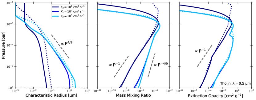
Figure 1: Vertical haze distributions for different eddy diffusion coefficient. From left to right, each column shows the vertical distributions of the characteristic particle size, the haze mass mixing ratio, and extinction opacity for the tholin optical constants at $\lambda=0.5~{}{\rm\mu m}$, respectively. Different colored lines show the distributions for different $K_{\rm z}$ with haze mass flux $F={10}^{-12}~{}{\rm g~{}{cm}^{-2}~{}s^{-1}}$. Dotted lines denote the distributions of a volume-weighted particle size predicted by a bin scheme for $K_{\rm z}={10}^{5}$ and ${10}^{9}~{}{\rm{cm}^{2}~{}s^{-1}}$ taken from Figure 17 of Kawashima & Ikoma (2019), where the column-integrated photolysis rate of haze precursors is $\sim{10}^{-12}~{}{\rm g~{}{cm}^{2}~{}s^{-1}}$ (see their Table 1).

We conduct a series of the calculations for haze particle growth and synthetic transmission spectra. We utilize a two-moment microphysical model of Ohno & Okuzumi (2018) that takes into account the eddy diffusion, gravitational settling, and particle growth. The moment model suffices to examine whether haze can produce SRSs, as the model can capture the basic effects of haze formation on transmission spectra (Kawashima & Ikoma, 2018). We assume spherical particles with constant density of $1~{}{\rm g~{}{cm}^{-3}}$ and ignore the condensation of mineral vapors for the sake of simplicity. The monomer production profile is prescribed by a log-normal profile given by (Ormel & Min, 2019)

$$\dot{\rho}_{\rm haze}=\rho_{\rm g}g\frac{F}{\sigma P\sqrt{2\pi}}\exp{\left[-\frac{1}{2\sigma^{2}}\left(\ln{\frac{P}{P_{\rm*}}}\right)^{2}\right]},$$ (10)

where the characteristic height of monomer production $P_{\rm*}$ and the width of the distribution $\sigma$ are set to $P_{\rm*}={10}^{-6}~{}{\rm bar}$ and $\sigma=0.5$ to mimic the profile predicted by photochemical models (e.g., Kawashima & Ikoma, 2019). Correspondingly, we include the increase of a particle number density as $\dot{n}_{\rm haze}=3\dot{\rho}_{\rm haze}/4\pi a_{\rm 0}^{3}\rho_{\rm p}$, where $a_{\rm 0}$ is the monomer radius and assumed to be $a_{\rm 0}=1~{}{\rm nm}$. The pressure-temperature structure for a solar composition atmosphere is constructed by an analytical model of Guillot (2010) using the same parameters adopted in Kawashima & Ikoma (2019) for their case of irradiation temperature of $790~{}{\rm K}$ .

We compute synthetic transmission spectra of hazy atmospheres using a model of Ohno et al. (2020) assuming the planetary mass of GJ 1214b ($6.26M_{\rm Earth}$, Anglada-Escudé et al., 2013) and the reference radius of $R_{\rm 0}=2.35R_{\rm Earth}$ at $P=10~{}{\rm bar}$. We introduce a metric quantifying steepness of the spectral slopes defined as (Pinhas & Madhusudhan, 2017)

$$\mathcal{S}\equiv\frac{1}{H}\frac{dR_{\rm p}}{d\ln{\lambda}}.$$ (11)

We use the $U$ band ($\lambda=365~{}{\rm nm}$, FWHM of $66~{}{\rm nm}$) and $V$ band ($\lambda=551~{}{\rm nm}$, FWHM of $88~{}{\rm nm}$) (Binney & Merrifield, 1998) to calculate $\mathcal{S}$, as similar to Pinhas & Madhusudhan (2017). The haze opacity is calculated by the BHMIE (Bohren & Huffman, 1983) assuming spherical particles. The refractive index has been unknown for exoplanetary haze. We test the two representative refractive index; a Titan haze analog (tholin, Khare et al., 1984) and a complex refractory hydrocarbon (soot) compiled by Lavvas & Koskinen (2017).

3.2 Haze Vertical Profiles

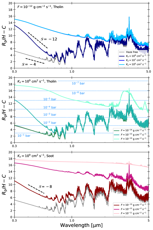
Figure 2: Synthetic transmission spectra of hazy atmospheres. The vertical axis is the planetary radius normalized by the scale height of $H=180~{}{\rm km}$, the value for $P\sim{10}^{-3}~{}{\rm bar}$, with an offset. The top panel shows the spectra for different $K_{\rm z}$ with $F={10}^{-12}~{}{\rm g~{}{cm}^{-2}~{}s^{-1}}$. The middle and bottom panels show the spectra for different $F$ with $K_{\rm z}={10}^{9}~{}{\rm{cm}^{-2}~{}s^{-1}}$. The tholin refractive index is assumed for the top and middle panels, while the soot refractive index is assumed for the bottom panel. Horizontal dotted lines in the middle panel denote the $R_{\rm p}/H-C$ corresponding to the pressure levels from ${10}^{-1}$ to ${10}^{-7}~{}{\rm bar}$.

Haze vertical distributions substantially vary with altitude, as suggested by previous studies (e.g., Lavvas & Koskinen, 2017; Kawashima & Ikoma, 2018, 2019; Kawashima et al., 2019; Adams et al., 2019; Lavvas et al., 2019; Gao & Zhang, 2020). Figure 1 shows the vertical distributions of haze characteristic size and mass mixing ratio for $F={10}^{-12}~{}{\rm g~{}{cm}^{-2}~{}s^{-1}}$ and different $K_{\rm z}$. We have confirmed that our two-moment model well reproduces the distributions simulated by the bin scheme (dotted lines) taken from Kawashima & Ikoma (2019). In principle, the particle size increases with decreasing the altitude because of collisional growth. The higher eddy diffusion coefficient is, the smaller particle size is. This is because efficient vertical mixing transports the particles downward before they grow into large sizes (Kawashima & Ikoma, 2019). The high eddy diffusion coefficient also produces a steep vertical gradient in the mass mixing ratio, as seen in the case of $K_{\rm z}={10}^{9}~{}{\rm{cm}^{2}~{}s^{-1}}$. This results in the steep vertical opacity gradient, as predicted in Section 2.

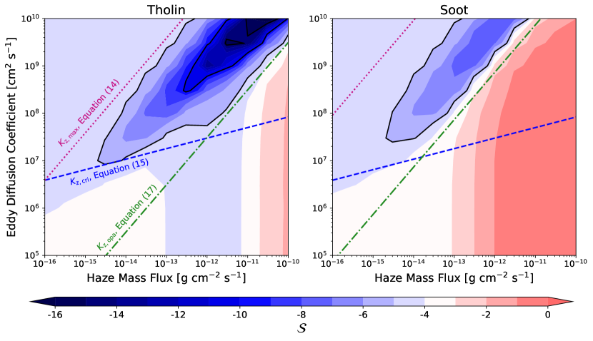
Figure 3: Gradient of the spectral slopes ($\mathcal{S}$, colorscale) as a function of eddy diffusion coefficient and haze mass flux. The left and right panels show the results for the tholin and soot haze, respectively. The black lines denote the contours of $\mathcal{S}=-5$, $-10$, and $-15$. The red dotted, blue dashed, and green broken lines denote Equations (14), (3.4), and (17), respectively, for $P=1~{}{\rm mbar}$ and $\lambda=0.55~{}{\rm\mu m}$. Here, we adopt the Rayleigh scattering cross section of a H₂ molecule, $\sigma_{\rm gas}=2.52\times{10}^{-28}~{}{\rm{cm}^{2}}~{}(\lambda/0.75~{}{\rm\mu m})^{-4}$ (Lecavelier Des Etangs et al., 2008), to evaluate the gas opacity.

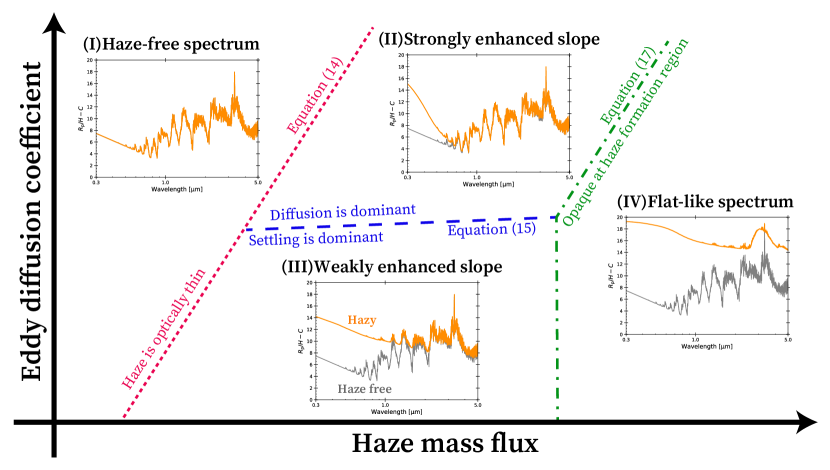
Figure 4: Transmission spectrum regimes in terms of haze mass flux and eddy diffusion coefficient (see Section 3.4). Each panel exhibits the typical shape of the transmission spectrum for hazy atmospheres (orange lines) compared to the haze-free spectrum (gray lines).

The vertical opacity gradient also appears when the settling dominates over the eddy diffusion, as seen in the cases of $K_{\rm z}={10}^{7}$ and ${10}^{5}~{}{\rm{cm}^{2}~{}s^{-1}}$. This is because the particle size is larger in the deeper atmosphere due to collisional growth, leading to yield vertical gradient in the mass mixing ratio. The vertical distributions can be further understood from a timescale argument. The particle can grow until the settling timescale, $\tau_{\rm settl}=H/v_{\rm t}$, becomes shorter than collisional timescale. For particles smaller than gas mean free path, the collision timescale is approximated by (e.g., Rossow, 1978)

$$\tau_{\rm coll}\approx\frac{1}{4}\sqrt{\frac{\rho_{\rm p}}{3ak_{\rm B}T}}\frac{m_{\rm haze}}{\rho_{\rm haze}}=\frac{1}{4}\sqrt{\frac{\rho_{\rm p}}{3ak_{\rm B}T}}\frac{m_{\rm haze}v_{\rm t}}{F},$$ (12)

where we have invoked the mass conservation $\rho_{\rm haze}v_{\rm t}=F$. Solving $\tau_{\rm coll}=\tau_{\rm sett}$ with Equation (8), the size is estimated as

$$a = \left(\frac{24FP^{2}}{\pi^{2}\rho_{\rm p}^{3}g^{3}}\sqrt{\frac{3k_{\rm B}T}{\rho_{\rm p}}}\right)^{2/9}$$ (13)

Equation (13) indicates that the particle size is proportional to $P^{4/9}$, which is indeed seen in Figure 1. Therefore, the mass mixing ratio is proportional to $P^{-4/9}$ for small $K_{\rm z}$ regimes (see Eqs. (8) and (A2)), resulting in the opacity higher at the higher altitude. In summary, the haze opacity is higher at higher altitude for all $K_{\rm z}$.

3.3 Transmission Spectra

The haze steepens the spectral slope for high $K_{\rm z}$, as found by Kawashima & Ikoma (2019). The top panel of Figure 2 shows the synthetic transmission spectra for various $K_{\rm z}$ assuming the tholin optical constants. For the tcase of $K_{\rm z}={10}^{9}~{}{\rm{cm}^{2}~{}s^{-1}}$, haze produces the spectral slope characterized by $\mathcal{S}\approx-12$ in the optical wavelength, quite steeper than the canonical Rayleigh slope ($\mathcal{S}=-4$). This stems from the vertical mass gradient produced by efficient eddy diffusion (Section 3.2). The spectra for $K_{\rm z}={10}^{7}$ and ${10}^{5}~{}{\rm{cm}^{2}~{}s^{-1}}$ are nearly superposed each other, as the vertical distributions are nearly the same.

The haze steepens the spectral slope only when the mass flux falls into a moderate value. As shown in the middle panel of Figure 2, the steep slope disappears in both cases of high and low mass flux. The low mass flux ($F={10}^{-14}~{}{\rm g~{}{cm}^{-2}~{}s^{-1}}$) leads to produce a spectrum superposed on a haze-free spectrum because the haze becomes optically thin as compared to the Rayleigh scattering opacity of H₂. By contrast, the high mass flux ($F={10}^{-10}~{}{\rm g~{}{cm}^{-2}~{}s^{-1}}$) leads to flatten the spectrum because the haze becomes optically thick near the monomer-formation region ($\sim{10}^{-6}~{}{\rm bar}$) up to a relatively long wavelength.

The spectral slope also depends on the optical constants. The bottom panel of Figure 2 shows the spectra calculated with the soot optical constants. The soot haze tends to flatten the spectra owing to the weak wavelength dependence of its absorption opacity. Although the slope is relatively gentle, the soot haze still produces the SRSs with $\mathcal{S}\approx-8$ for $K_{\rm z}={10}^{9}~{}{\rm{cm}^{2}~{}s^{-1}}$ and $F={10}^{-11}~{}{\rm g~{}{cm}^{-2}~{}s^{-1}}$.

3.4 In what conditions haze produces SRSs?

There is a “sweet spot” in the $F$–$K_{\rm z}$ space to produce the SRSs. Figure 3 summarizes the spectral slopes calculated for $U$-$V$ bands as a function of haze mass flux $F$ and eddy diffusion coefficient $K_{\rm z}$. The slopes are relatively flat (i.e., $\mathcal{S}\sim 0$) for very high $F$, as the haze becomes optically thick near the monomer formation region (Section 3.3). By contrast, low $F$ and high $K_{\rm z}$ tend to yield $\mathcal{S}=-4$, as the haze becomes optically thin. For moderate mass flux, say $F\gtrsim{10}^{-14}~{}{\rm g~{}{cm}^{-2}~{}s^{-1}}$, the slopes have $\mathcal{S}\sim-4$ for $K_{\rm z}\lesssim{10}^{7}~{}{\rm{cm}^{2}~{}s^{-1}}$ and $\mathcal{S}<-5$ for $K_{\rm z}\gtrsim{10}^{7}~{}{\rm{cm}^{2}~{}s^{-1}}$. The steep spectral slope (i.e., small $\mathcal{S}$) for high $K_{\rm z}$ stems from the steep vertical gradient in the mass mixing ratio (Section 3.2). In the parameter space examined here, the most steep slope has $\mathcal{S}\approx-16$ for the tholin haze and $\mathcal{S}\approx-8$ for the soot haze, which is found for $F\sim{10}^{-12}$–${10}^{-11}~{}{\rm g~{}{cm}^{-2}~{}s^{-1}}$ and $K_{\rm z}\sim{10}^{10}~{}{\rm{cm}^{2}~{}s^{-1}}$.

The transmission spectra of hazy atmospheres can be demarcated into four typical regimes as presented in Figure 4. When $K_{\rm z}$ is extremely high, the haze becomes optically thin as compared to gas opacity, resulting in a haze-free spectrum (regime I). Equating Equation (7) and the gas opacity $\kappa_{\rm gas}$ with $v_{\rm t}H/K{\rm z}\ll 1$, the threshold $K_{\rm z}$ above which the regime I applies is given by

$$K_{\rm z,max}=\frac{36\pi gH^{2}F}{\rho_{\rm p}\kappa_{\rm gas}P}\frac{nk\lambda^{-1}}{(n^{2}-k^{2}+2)^{2}+(2nk)^{2}}.$$ (14)

For $K_{\rm z}<K_{\rm z,max}$, the spectrum is substantially affected by haze. The spectral slope is significantly enhanced by haze when the eddy diffusion dominates over the settling of haze particles (regime II). Conversely, the slope is only weakly enhanced if the settling dominates over the eddy diffusion (regime III). Solving $\tau_{\rm diff}=\tau_{\rm sett}$ with Equations (8) and (13), where $\tau_{\rm diff}=H^{2}/K_{\rm z}$ is the diffusion timescale, the critical $K_{\rm z}$ above which eddy diffusion dominates over the settling is estimated as

$$K_{\rm z,cri} = \frac{\rho_{\rm p}g^{2}H^{2}}{P\sqrt{8gH/\pi}}\left(\frac{24FP^{2}}{\pi^{2}\rho_{\rm p}^{3}g^{3}}\sqrt{\frac{3k_{\rm B}T}{\rho_{\rm p}}}\right)^{2/9}$$

$$\sim 3\times{10}^{7}~{}{\rm{cm}^{2}~{}s^{-1}}~{}\left(\frac{F}{{10}^{-12}~{}{\rm g~{}{cm}^{2}~{}s^{-1}}}\right)^{2/9}\left(\frac{H}{{200}~{}{\rm km}}\right)^{3/2}$$

$$\times\left(\frac{g}{{10}~{}{\rm m~{}s^{-2}}}\right)^{5/6}\left(\frac{P}{{1}~{}{\rm mbar}}\right)^{-5/9}\left(\frac{T}{{1000}~{}{\rm K}}\right)^{1/9}\left(\frac{\rho_{\rm p}}{{1}~{}{\rm g~{}{cm}^{-3}}}\right)^{2/9}.$$

The spectrum eventually becomes flat when the mass flux is so high that haze is optically thick at the monomer formation region (regime IV). Since the vertical mass distribution does not follow a power law near the monomer formation region (see Figure 1), we crudely evaluate the optical depth as

$$\tau_{\rm s}(P_{\rm*})\sim\frac{P_{\rm*}}{gH}\kappa(P_{\rm*})\sqrt{2\pi R_{\rm p}H}.$$ (16)

Inserting Equation (7) into (16) and solving $\tau_{\rm s}(P_{\rm*})=1$ with $v_{\rm t}H/K_{\rm z}\ll 1$, we achieve the threshold in terms of $K_{\rm z}$ as

$$K_{\rm z,opa}=\frac{36\pi HF\sqrt{2\pi R_{\rm p}H}}{\rho_{\rm p}}\frac{nk\lambda^{-1}}{(n^{2}-k^{2}+2)^{2}+(2nk)^{2}}$$ (17)

Equation (17) does not apply when the settling dominates over the eddy diffusion, i.e., $K_{\rm z}<K_{\rm z,cri}$. Since the spectrum is invariant with $K_{\rm z}$ for the settling-dominated regime (see Figure 2), the threshold for $K_{\rm z}<K_{\rm z,cri}$ is given as an intersection of Equations (3.4) and (17). We plot Equations (14), (3.4), and (17) in Figure 3 and find that the regime classification well explains the basic behavior of spectral slopes. Notably, the SRSs preferentially emerge in the regime II (see Figure 4), where the eddy diffusion coefficient falls into the sweet spot, namely ${\rm max}(K_{\rm z,cri},K_{\rm z,opa})<K_{\rm z}<K_{\rm z,max}$. Alternatively, the SRSs emerge when the haze mass flux falls into a moderate value for given $K_{\rm z}$; for example, $F\sim{10}^{-13}$–${10}^{-11}~{}{\rm g~{}{cm}^{-2}~{}s^{-1}}$ for $K_{\rm z}={10}^{9}~{}{\rm{cm}^{2}~{}s^{-1}}$ (see Figure 3). Thus, the SRSs might give a constraint on haze mass flux if the strength of eddy diffusion is well constrained.

4 Summary and Discussion

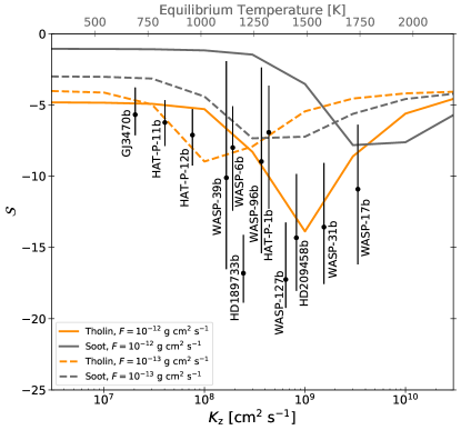
Figure 5: Haze-generated spectral slopes as a function of $K_{\rm z}$. The solid and dashed lines show the slopes for $F={10}^{-12}$ and ${10}^{-13}~{}{\rm g~{}{cm}^{2}~{}s^{-1}}$, respectively, which are in line with the predictions from column integrated photolysis rate of hydrocarbons reported by previous studies (Lavvas & Koskinen, 2017; Kawashima & Ikoma, 2019). The orange and gray lines exhibit the slopes for tholin and soot haze, respectively. The black dots denote the slopes retrieved by Welbanks et al. (2019) with $1\sigma$ error bars.

In this study, we have suggested that the super-Rayleigh slopes seen in transmission spectra of some exoplanets can be produced by photochemical haze. We have analytically shown that the spectral slope is steepened by the vertical gradient of atmospheric opacity, which is naturally generated by haze (Section 2). We have numerically confirmed that the haze can produce the spectral slope several times steeper than the canonical Rayleigh slope, especially when the eddy diffusion coefficient and the haze mass flux fall into the sweet spot (Section 3). We have also demarcated the transmission spectra of hazy atmospheres into four typical regimes (Figure 4). Our results would help to not only interpret the SRSs but also figure out how haze affects the transmission spectra.

One of the possible approaches for testing our idea is to search for the absorption feature of haze itself. For instance, Titan tholin exhibits absorption features at $3.0$, $4.6$, and $6.3~{}{\rm{\mu}m}$ (e.g., Khare et al., 1984; Imanaka et al., 2004). It may be worth investigating whether planets with SRSs show the features at these wavelength. The actual optical constants of exoplanetary hazes have been unknown. Therefore, laboratory studies on exoplanetary haze analogs (e.g., Hörst et al., 2018; He et al., 2018; Moran et al., 2020) are important to examine what optical constants are more plausible for exoplanet environments. The reliable optical constants will also help to quantify the effects of hazes on the spectral slopes.

There may be a “sweet spot” of planetary equilibrium temperature in which haze preferentially causes the SRSs. This is because the equilibrium temperature is associated with $K_{\rm z}$ (Komacek et al., 2019). Figure 5 shows the spectral slope $\mathcal{S}$ as a function of $K_{\rm z}$ and corresponding equilibrium temperature, where we have assumed a following relation

$$\log{{}_{\rm 10}(K_{\rm z}~{}{\rm[m^{2}~{}s^{-1}])}}=2.110\left(\frac{T_{\rm eq}}{1000~{}{\rm K}}\right)+1.855.$$ (18)

This relation is obtained by a linear fit to $K_{\rm z}$ simulated by Komacek et al. (2019) for drag-free atmospheres with $0.01~{}{\rm\mu m}$ passive tracers at $P=1~{}{\rm mbar}$ (their Figure 8). Haze preferentially produce steep slopes at equilibrium temperature of $\sim 1000$–$1500~{}{\rm K}$ in which $K_{\rm z}$ falls into the regime II. Figure 5 also exhibits the slope retrieved by Welbanks et al. (2019) (their $\gamma$). Interestingly, in the retrieval results, planets with equilibrium temperature of $\sim 1200$–$1400~{}{\rm K}$ tend to exhibit steep spectral slopes, as similar to the haze-generated SRSs. We do not claim that the result verifies the haze hypotheses since there are many uncertainties, such as stellar contamination (e.g., McCullough et al., 2014) and multi-dimension effects (e.g., Caldas et al., 2019; MacDonald et al., 2020), that should be assessed in future. Rather, we suggest that measuring the spectral slopes for various equilibrium temperature can help to investigate whether the SRSs are predominantly caused by haze.

Photochemical haze also complements the model of mineral clouds. Current cloud microphysical models do not predict the optical spectral slope as steep as the Rayleigh slope (Gao & Benneke, 2018; Lines et al., 2018; Lee et al., 2019; Powell et al., 2019; Ohno et al., 2020), except for Ormel & Min (2019) who showed some cases that succeeded in producing the steep spectral slopes. Although it has been believed that haze formation is inefficient in hot exoplanets where CH₄ is oxidized to CO (Zahnle et al., 2009a), recent laboratory studies suggest that CO also act as haze precursors (Hörst et al., 2018; He et al., 2019). Thus, haze may still be responsible for hot exoplanets that often show spectral slopes in their transmission spectra.

Appendix A Derivation of Analytical Haze Opacity

In this appendix, we derive the vertical distribution of atmospheric opacity including haze. The steady vertical distribution of haze mass density $\rho_{\rm haze}$ is determined by the mass conservation, which reads

$$\frac{K_{\rm z}}{gH^{2}}P^{2}\frac{\partial}{\partial P}\left(\frac{\rho_{\rm haze}}{\rho_{\rm g}}\right)-v_{\rm t}\rho_{\rm haze}=-F,$$ (A1)

where we have used the hydrostatic equilibrium, the ideal gas law, and the definition of $H$. In the upper atmospheres where haze particles are much smaller than gas mean free path, the terminal velocity can be approximated by Equation (8). For constant $K_{\rm z}$, $\rho_{\rm p}$, and $a$, Equation (A1) is solved as

$$\frac{\rho_{\rm haze}}{\rho_{\rm g}}=\frac{gHF}{Pv_{\rm t}}\left[1-\exp{\left(-\frac{v_{\rm t}H}{K_{\rm z}}\right)}\right],$$ (A2)

where we have set the boundary condition of $\rho_{\rm haze}=0$ at $P=\infty$. The extinction cross sections of haze particles may be approximated by absorption cross section, especially for particles much smaller than relevant wavelength. For such tiny particles, the absorption cross section is approximated by (Bohren & Huffman, 1983; Kataoka et al., 2014)

$$\sigma_{\rm abs}\approx\pi a^{2}\frac{24nk}{(n^{2}-k^{2}+2)^{2}+(2nk)^{2}}\frac{2\pi a}{\lambda}.$$ (A3)

Combining Equations (A2) and (A3), we finally achieve the opacity (Equation 7) as

$$\kappa = \frac{3\sigma_{\rm abs}}{4\pi a^{3}\rho_{\rm p}}\frac{\rho_{\rm haze}}{\rho_{\rm g}}$$

$$= \frac{36\pi gHF}{\rho_{\rm p}}{\underbrace{\frac{1}{Pv_{\rm t}}\left[1-\exp{\left(-\frac{v_{\rm t}H}{K_{\rm z}}\right)}\right]}_{\text{Pressuredependence}}}\underbrace{\frac{nk\lambda^{-1}}{(n^{2}-k^{2}+2)^{2}+(2nk)^{2}}}_{\text{Wavelengthdependence}},$$

Equation (A) demonstrates that, for tiny absorbing haze, the pressure dependence is originated from the vertical mass gradient, while the wavelength dependence is from haze optical constants.

References

- Adams et al. (2019) Adams, D., Gao, P., de Pater, I., & Morley, C. V. 2019, ApJ, 874, 61
- Anglada-Escudé et al. (2013) Anglada-Escudé, G., Rojas-Ayala, B., Boss, A. P., Weinberger, A. J., & Lloyd, J. P. 2013, A&A, 551, A48
- Benneke & Seager (2012) Benneke, B., & Seager, S. 2012, ApJ, 753, 100
- Binney & Merrifield (1998) Binney, J., & Merrifield, M. 1998, Galactic Astronomy
- Bohren & Huffman (1983) Bohren, C. F., & Huffman, D. R. 1983, Absorption and scattering of light by small particles
- Caldas et al. (2019) Caldas, A., Leconte, J., Selsis, F., et al. 2019, A&A, 623, A161
- Charbonneau et al. (2002) Charbonneau, D., Brown, T. M., Noyes, R. W., & Gilliland, R. L. 2002, ApJ, 568, 377
- Espinoza et al. (2019) Espinoza, N., Rackham, B. V., Jordán, A., et al. 2019, MNRAS, 482, 2065
- Evans et al. (2018) Evans, T. M., Sing, D. K., Goyal, J. M., et al. 2018, AJ, 156, 283
- Fortney (2005) Fortney, J. J. 2005, MNRAS, 364, 649
- Gao & Benneke (2018) Gao, P., & Benneke, B. 2018, ApJ, 863, 165
- Gao & Zhang (2020) Gao, P., & Zhang, X. 2020, ApJ, 890, 93
- Guillot (2010) Guillot, T. 2010, A&A, 520, A27
- He et al. (2018) He, C., Hörst, S. M., Lewis, N. K., et al. 2018, ApJ, 856, L3
- He et al. (2019) —. 2019, ACS Earth and Space Chemistry, 3, 39
- Hörst et al. (2018) Hörst, S. M., He, C., Lewis, N. K., et al. 2018, Nature Astronomy, 2, 303
- Imanaka et al. (2004) Imanaka, H., Khare, B. N., Elsila, J. E., et al. 2004, Icarus, 168, 344
- Kataoka et al. (2014) Kataoka, A., Okuzumi, S., Tanaka, H., & Nomura, H. 2014, A&A, 568, A42
- Kawashima et al. (2019) Kawashima, Y., Hu, R., & Ikoma, M. 2019, ApJ, 876, L5
- Kawashima & Ikoma (2018) Kawashima, Y., & Ikoma, M. 2018, ApJ, 853, 7
- Kawashima & Ikoma (2019) —. 2019, ApJ, 877, 109
- Khare et al. (1984) Khare, B. N., Sagan, C., Arakawa, E. T., et al. 1984, Icarus, 60, 127
- Komacek et al. (2019) Komacek, T. D., Showman, A. P., & Parmentier, V. 2019, ApJ, 881, 152
- Kreidberg et al. (2014) Kreidberg, L., Bean, J. L., Désert, J.-M., et al. 2014, Nature, 505, 69
- Lavvas & Koskinen (2017) Lavvas, P., & Koskinen, T. 2017, ApJ, 847, 32
- Lavvas et al. (2019) Lavvas, P., Koskinen, T., Steinrueck, M. E., García Muñoz, A., & Showman, A. P. 2019, ApJ, 878, 118
- Lecavelier Des Etangs et al. (2008) Lecavelier Des Etangs, A., Pont, F., Vidal-Madjar, A., & Sing, D. 2008, A&A, 481, L83
- Lee et al. (2019) Lee, G. K. H., Taylor, J., Grimm, S. L., et al. 2019, MNRAS, 487, 2082
- Lines et al. (2018) Lines, S., Manners, J., Mayne, N. J., et al. 2018, MNRAS, 481, 194
- MacDonald et al. (2020) MacDonald, R. J., Goyal, J. M., & Lewis, N. K. 2020, arXiv e-prints, arXiv:2003.11548
- May et al. (2020) May, E. M., Gardner, T., Rauscher, E., & Monnier, J. D. 2020, AJ, 159, 7
- McCullough et al. (2014) McCullough, P. R., Crouzet, N., Deming, D., & Madhusudhan, N. 2014, ApJ, 791, 55
- Moran et al. (2020) Moran, S. E., Hörst, S. M., Vuitton, V., et al. 2020, arXiv e-prints, arXiv:2004.13794
- Ohno & Okuzumi (2018) Ohno, K., & Okuzumi, S. 2018, ApJ, 859, 34
- Ohno et al. (2020) Ohno, K., Okuzumi, S., & Tazaki, R. 2020, ApJ, 891, 131
- Ormel & Min (2019) Ormel, C. W., & Min, M. 2019, A&A, 622, A121
- Pinhas & Madhusudhan (2017) Pinhas, A., & Madhusudhan, N. 2017, MNRAS, 471, 4355
- Pinhas et al. (2019) Pinhas, A., Madhusudhan, N., Gandhi, S., & MacDonald, R. 2019, MNRAS, 482, 1485
- Pont et al. (2013) Pont, F., Sing, D. K., Gibson, N. P., et al. 2013, MNRAS, 432, 2917
- Powell et al. (2019) Powell, D., Louden, T., Kreidberg, L., et al. 2019, ApJ, 887, 170
- Rossow (1978) Rossow, W. B. 1978, Icarus, 36, 1
- Sedaghati et al. (2017) Sedaghati, E., Boffin, H. M. J., MacDonald, R. J., et al. 2017, Nature, 549, 238
- Sing et al. (2016) Sing, D. K., Fortney, J. J., Nikolov, N., et al. 2016, Nature, 529, 59
- Welbanks et al. (2019) Welbanks, L., Madhusudhan, N., Allard, N. F., et al. 2019, ApJ, 887, L20
- Woitke & Helling (2003) Woitke, P., & Helling, C. 2003, A&A, 399, 297
- Zahnle et al. (2009a) Zahnle, K., Marley, M. S., & Fortney, J. J. 2009a, arXiv e-prints, arXiv:0911.0728
- Zahnle et al. (2009b) Zahnle, K., Marley, M. S., Freedman, R. S., Lodders, K., & Fortney, J. J. 2009b, ApJ, 701, L20