Diffusivity Estimation for Activator-Inhibitor Models: Theory and Application to Intracellular Dynamics of the Actin Cytoskeleton

Abstract.

A theory for diffusivity estimation for spatially extended activator-inhibitor dynamics modelling the evolution of intracellular signaling networks is developed in the mathematical framework of stochastic reaction-diffusion systems. In order to account for model uncertainties, we extend the results for parameter estimation for semilinear stochastic partial differential equations, as developed in [PS20], to the problem of joint estimation of diffusivity and parametrized reaction terms. Our theoretical findings are applied to the estimation of effective diffusivity of signaling components contributing to intracellular dynamics of the actin cytoskeleton in the model organism Dictyostelium discoideum.

1. Introduction

The purpose of this paper is to develop the mathematical theory for statistical inference methods for the parameter estimation of stochastic reaction-diffusion systems modelling spatially extended signaling networks in cellular systems. Such signaling networks are one of the central topics in cell biology and biophysics as they provide the basis for essential processes including cell division, cell differentiation, and cell motility [DBE⁺17]. Nonlinearities in these network may cause rich spatiotemporal behavior including the emergence of oscillations and waves [BK17]. Furthermore, alterations and deficiencies in the network topology can explain many pathologies and play a key role in diseases such as cancer [CSS05]. Here we present a method to estimate both diffusivity and reaction terms of a stochastic reaction-diffusion system, given space-time structured data of local concentrations of signaling components. We mainly focus on the estimation of diffusivity, whose precision can be increased by simultaneous calibration of the reaction terms. To test this approach, we use fluorescence microscopy recordings of the actin dynamics in the cortex of cells of the social amoeba Dictyostelium discoideum, a well-established model organism for the study of a wide range of actin-dependent processes [AF09]. A recently introduced stochastic reaction-diffusion model could reproduce many features of the dynamical patterns observed in the cortex of these cells including excitable and bistable states [ASB18, FFAB20, MFF⁺20]. In combination with the experimental data, this model will serve as a specific test case to exemplify our mathematical approach. Since in real-world applications the available data will not allow for calibrating and validating detailed mathematical models, in this paper we will be primarily interested in minimal models that are still capable of generating all observed dynamical features at correct physical magnitudes. The developed estimation techniques should in practice be as robust as possible w.r.t. uncertainty and even misspecification of the unknown real dynamics.

The impact of diffusion and reaction in a given model will be of fundamentally different structure and it is one of the main mathematical challenges to separate these impacts in the data in order to come to valid parameter estimations. On the more mathematical side, diffusion corresponds to a second order partial differential operator — resulting in a strong spatial coupling in the given data, whereas the reaction corresponds to a lower order, in fact $0$-order, in general resulting in highly nonlinear local interactions in the data. For introductory purposes, let us assume that our data is given in terms of a space and time-continuous field $X(t,x)$ on $[0,T]\times\mathcal{D}$, where $T$ is the terminal time of our observations and $\mathcal{D}\subset\mathbb{R}^{2}$ a rectangular domain that corresponds to a chosen data-segment in a given experiment. Although in practice the given data will be discrete w.r.t. both space and time, we will be interested in applications where the resolution is high enough in order to approximate the data by such a continuous field. Our standing assumption is that $X(t,x)$ is generated by a dynamical system of the form

(1) $$\partial_{t}X(t,x)=\theta_{0}\Delta X(t,x)+\mathcal{F}_{X}(t,x),$$

where $\Delta$ is the Laplacian, given by $\Delta X(t,x)=\partial_{x_{1}}^{2}X(t,x)+\partial_{x_{2}}^{2}X(t,x)$, $x=(x_{1},x_{2})$, which captures the diffusive spreading in the dynamics of $X(t,x)$. The intensity of the diffusion is given by the diffusivity $\theta_{0}$. Finally, $\mathcal{F}$ is a generic term, depending on the solution field $X(t,x)$, which describes all non-diffusive effects present in $X(t,x)$, whether they are known or unknown. A natural approach to extract $\theta_{0}$ from the data is to use a “cutting-out estimator” of the form

(2) $$\hat{\theta}_{0}=\frac{\int_{0}^{T}\int_{\mathcal{D}}Y(t,x)\partial_{t}X(t,x)\mathrm{d}x\mathrm{d}t}{\int_{0}^{T}\int_{\mathcal{D}}Y(t,x)\Delta X(t,x)\mathrm{d}x\mathrm{d}t}=\frac{\int_{0}^{T}\langle Y,\partial_{t}X\rangle\mathrm{d}t}{\int_{0}^{T}\langle Y,\Delta X\rangle\mathrm{d}t},$$

where $Y(t,x)$ is a suitable test function. In the second fraction of (2), we use the functional form for readability. In particular, we write $X=X(t,x)$ for the solution field. We will also write $X_{t}=X(t,\cdot)$ for the (spatially varying) solution field at a fixed time $t$. In order to ease notation, we will use this functional form from now on throughout the paper. It is possible to derive (2) from a least squares approach by minimizing $\theta\mapsto\lVert\partial_{t}X-\theta\Delta X\rVert^{2}$ with a suitably chosen norm. If the non-diffusive effects described by $\mathcal{F}$ are negligible, we see by plugging (1) into (2) that $\hat{\theta}_{0}$ is close to $\theta_{0}$. If a sound approximation $\overline{\mathcal{F}}$ to $\mathcal{F}$ is known, the estimator can be made more precise by substituting $\partial_{t}X$ by $\partial_{t}X-\overline{\mathcal{F}}_{X}$ in (2). A usual choice for $Y$ is a reweighted spectral cutoff of $X$.

Under additional model assumptions, e.g. if (1) is in fact a stochastic partial differential equation (SPDE) driven by Gaussian white noise, a rather developed parameter estimation theory for $\theta_{0}$ has been established in [PS20] on the basis of maximum likelihood estimation (MLE).

In this paper, we are interested in further taking into account also those parts of $\mathcal{F}_{X}$ corresponding to local nonlinear reactions. As a particular example, we will focus on a recently introduced stochastic reaction-diffusion system of FitzHugh–Nagumo type that captures many aspects of the dynamical wave patterns observed in the cortex of motile amoeboid cells [FFAB20],

(3) $$\partial_{t}U =D_{U}\Delta U+k_{1}U(u_{0}-U)(U-u_{0}a)-k_{2}V+\xi,$$

(4) $$\partial_{t}V =D_{V}\Delta V+\epsilon(bU-V).$$

Here, we identify $\theta_{0}=D_{U}$ and the only observed data is the activator variable, i.e. $X=U$.

Therefore, in this example the non-diffusive part of the dynamics will be further decomposed as $\mathcal{F}=F+\xi$, where $\xi$ is Gaussian white noise and $F=F(U)$ encodes the non-Markovian reaction dynamics of the activator. The inhibitor component $V$ in the above reaction-diffusion system is then incorporated for minimal modelling purposes to allow the formation of travelling waves in the activator variable $U$ that are indeed observed in the time evolution of the actin concentration. This model and its dynamical features is explained in detail in Section 2.1.1.

As noted before, it is desirable to include this additional knowledge into the estimation procedure (2) by subtracting a suitable approximation $\overline{\mathcal{F}}$ of the — in practice — unknown $\mathcal{F}$. Although (3), (4) suggest an explicit parametric form for $\overline{\mathcal{F}}$, it is a priori not clear how to quantify the nuisance parameters appearing in the system. Thus an (approximate) model for the data is known qualitatively, based on the observed dynamics, but not quantitatively. In order to resolve this issue, we extend (2) and adopt a joint maximum likelihood estimation of $\theta_{0}$ and various nuisance parameters.

The field of statistical inference for SPDEs is rapidly growing, see [Cia18] for a recent survey. The spectral approach to drift estimation was pioneered by [HKR93, HR95] and subsequently extended by various works, see e.g. [HLR97, LR99, LR00] for the case of non-diagonalizable linear evolution equations. In [CGH11], the stochastic Navier-Stokes equations have been analyzed as a first example of a nonlinear evolution equation. This has been generalized by [PS20] to semilinear SPDEs. Joint parameter estimation for linear evolution equations is treated in [Hue93, Lot03]. Besides the spectral approach, other measurement schemes have been studied. See e.g. [PT07, BT20, BT19, Cho19a, Cho19b, KT19, CH19, CDVK20, CK20, KU19] for the case of discrete observations in space and time. Recently, the so-called local approach has been worked out in [AR20] for linear equations, was subsequently generalized in [ACP20] to the semilinear case and applied to a stochastic cell repolarization model in [ABJR20].

The paper is structured as follows: In Section 2 we give a theory for joint diffusivity and reaction parameter estimation for a class of semilinear SPDEs and study the spatial high-frequency asymptotics. In Section 3, the biophysical context for these models is discussed. The performance of our method on simulated and real data is evaluated in Section 4.

2. Maximum Likelihood Estimation for
Activator-Inhibitor Models

In this section we develop a theory for parameter estimation for a class of semilinear SPDE using a maximum likelihood ansatz. The application we are aiming at is an activator-inhibitor model as in [FFAB20]. More precisely, we show under mild conditions that the diffusivity of such a system can be identified in finite time given high spatial resolution and observing only the activator component.

2.1. The Model and Basic Properties

Let us first introduce the abstract mathematical setting in which we are going to derive our main theoretical results. We work in spatial dimension $d\geq 1$. Given a bounded domain $\mathcal{D}=[0,L_{1}]\times\dots\times[0,L_{d}]\subset\mathbb{R}^{d}$, $L_{1},\dots,L_{d}>0$, we consider the following parameter estimation problem for the semilinear SPDE

(5) $$\mathrm{d}X_{t}=\left(\theta_{0}\Delta X_{t}+F_{\theta_{1},\dots,\theta_{K}}(X)\right)\mathrm{d}t+B\mathrm{d}W_{t}$$

with periodic boundary conditions for $\Delta$ on the Hilbert space $H=\bar{L}^{2}(\mathcal{D})=\{u\in L^{2}(\mathcal{D})|\int_{\mathcal{D}}u\mathrm{d}x=0\}$, together with initial condition $X_{0}\in H$. We allow the nonlinear term $F$ to depend on additional (nuisance) parameters $\theta_{1},\dots,\theta_{K}$ and write $\theta=(\theta_{0},\dots,\theta_{K})^{T}$, $\theta_{1:K}=(\theta_{1},\dots,\theta_{K})$ for short. Without further mentioning it, we assume that $\theta\in\Theta$ for a fixed parameter space $\Theta$, e.g. $\Theta=\mathbb{R}_{+}^{K}$. Next, $W$ is a cylindrical Wiener process modelling Gaussian space-time white noise, that is, $\mathbb{E}[\dot{W}(t,x)]=0$ and $\mathbb{E}[\dot{W}(t,x)\dot{W}(s,y)]=\delta(t-s)\delta(x-y)$. In order to introduce spatial correlation, we use a dispersion operator of the form $B=\sigma(-\Delta)^{-\gamma}$ with $\sigma>0$ and $\gamma>d/4$. Here, $\sigma$ is the noise intensity, and $\gamma$ quantifies the decay of the noise for large frequencies in Fourier space. In addition, $\gamma$ determines the spatial smoothness of $X$, see Section 2.1.2. The condition $\gamma>d/4$ ensures that the covariance operator $BB^{T}$ is of trace class, which is a standard assumption for well-posedness of (5), cf. [LR15]. Denote by $(\lambda_{k})_{k\geq 0}$ the eigenvalues of $-\Delta$, ordered increasingly, with corresponding eigenfunctions $(\Phi_{k})_{k\geq 0}$. It is well-known [Wey11, Shu01] that $\lambda_{k}\asymp\Lambda k^{2/d}$ for a constant $\Lambda>0$, i.e. $\lim_{k\rightarrow\infty}\lambda_{k}/(\Lambda k^{2/d})=1$. The proportionality constant $\Lambda$ is known explicitly (see e.g. [Shu01, Proposition 13.1]) and depends on the domain $\mathcal{D}$. Let $P_{N}:H\rightarrow H$ be the projection onto the span of the first $N$ eigenfunctions, and set $X^{N}:=P_{N}X$. For later use, we denote by $I$ the identity operator acting on $H$. For $s\in\mathbb{R}$, we write $H^{s}:=D((-\Delta)^{s/2})$ for the domain of $(-\Delta)^{s/2}$, which is given by

$$(-\Delta)^{s/2}x=\sum_{k=1}^{\infty}\lambda_{k}^{s/2}\langle\Phi_{k},x\rangle\Phi_{k},$$

and abbreviate $|\cdot|_{s}:=|\cdot|_{H^{s}}$ for the norm on that space whenever convenient. We assume that the initial condition $X_{0}$ is regular enough, i.e. it satisfies $\mathbb{E}[|X_{0}|_{s}^{p}]<\infty$ for any $s\geq 0$, $p\geq 1$, without further mentioning it in the forthcoming statements. We will use the following general class of conditions with $s\geq 0$ in order to describe the regularity of $X$:

• For any $p\geq 1$, it holds

  (6) $$\mathbb{E}\left[\sup_{0\leq t\leq T}|X_{t}|_{s}^{p}\right]<\infty.$$

Our standing assumption is that there is a unique solution $X$ to (5) such that $(A_{0})$ holds. This is a general statement and can be derived e.g. under the assumptions from [LR15, Theorem 3.1.5].

2.1.1. An Activator-Inhibitor Model

An important example for our analysis is given by the following FitzHugh–Nagumo type system of equations in $d\leq 2$ (cf. [FFAB20]):

(7) $$\mathrm{d}U_{t} =(D_{U}\Delta U_{t}+k_{1}f(\lvert U_{t}\rvert_{L^{2}},U_{t})-k_{2}V_{t})\mathrm{d}t+B\mathrm{d}W_{t},$$

(8) $$\mathrm{d}V_{t} =(D_{V}\Delta V_{t}+\epsilon(bU_{t}-V_{t}))\mathrm{d}t,$$

together with sufficiently smooth initial conditions. Here, $f$ is a bistable third-order polynomial $f(x,u)=u(u_{0}-u)(u-a(x)u_{0})$, and $a\in C^{1}_{b}(\mathbb{R},\mathbb{R})$ is a bounded and continuously differentiable function with bounded derivative. The boundedness condition for $a$ is not essential to the dynamics of $U$ and can be realized in practice by a suitable cutoff function.

The FitzHugh–Nagumo system [Fit61, NAY62] originated as a minimal model capable of generating excitable pulses mimicking action potentials in neuroscience. Its two components $U$ and $V$ are called activator and inhibitor, resp.

The spatial extension of the Fitzhugh–Nagumo system, obtained via diffusive coupling, is used to model propagation of excitable pulses and two-phase dynamics. In the case of the two phases, low and high concentration of the activator $U$ are realized as the stable fixed points of the third order polynomial $f$ at $0$ and $u_{0}$. The unstable fixed point $au_{0}$, $a\in(0,1)$, separates the domains of attraction of the two stable fixed points. The interplay between spatial diffusion, causing a smoothing out of concentration gradients with rate $D_{U}$, and the local reaction forcing $f$, causing convergence of the activator to one of the stable phases with rate $k_{1}$, leads to the formation of transition phases between regions with low or high concentration of $U$. The parameters determine shape and velocity of the transition phases, e.g. low values of $a$ enhance the growth of regions with high activator concentration. This corresponds to the excitable regime, as explained in [FFAB20].

Conversely, a high concentration of the inhibitor $V$ leads to a decay in the activator $U$, with rate $k_{2}$. In the excitable regime, this mechanism leads to moving activator wave fronts. The inhibitor is generated with rate $\epsilon b$ in the presence of $U$ and decays at rate $\epsilon$. Finally, its spatial evolution is determined by diffusion with rate $D_{V}$.

Finally, choosing $a$ as a functional depending on the total activator concentration introduces a feedback control that allows to stabilize the dynamics.

A detailed discussion of the relevance for cell biology is given in Section 3. More information on the FitzHugh–Nagumo model and related models can be found in [ET10].

For this model, we can find a representation of the above type (5) as follows: Using the variation of constants formula, the solution $V$ to (8) with initial condition $V_{0}=0$ can be written as $V_{t}=\epsilon b\int_{0}^{t}e^{(t-r)(D_{V}\Delta-\epsilon I)}U_{r}\mathrm{d}r$. Inserting this representation into (7) yields the following reformulation

(9) $$\mathrm{d}U_{t} =\Big{(}D_{U}\Delta U_{t}+k_{1}U_{t}(u_{0}-U_{t})(U_{t}-au_{0})$$

$$\quad-k_{2}\epsilon b\int_{0}^{t}e^{(t-r)(D_{V}\Delta-\epsilon I)}U_{r}\mathrm{d}r\Big{)}\mathrm{d}t+B\mathrm{d}W_{t}$$

$$=\left(\theta_{0}\Delta U_{t}+\theta_{1}F_{1}(U_{t})+\theta_{2}F_{2}(U_{t})+\theta_{3}F_{3}(U)(t)\right)\mathrm{d}t+B\mathrm{d}W_{t}$$

of the activator-inhibitor model (7), (8) by setting $\theta_{0}=D_{U}$, $\theta_{1}=k_{1}u_{0}\bar{a}$, $\theta_{2}=k_{1}$, $\theta_{3}=k_{2}\epsilon b$, $\overline{F}=0$ for some $\bar{a}>0$ and

(10) $$F_{1}(U) =-\frac{a(|U|_{L^{2}})}{\bar{a}}U(u_{0}-U),$$

(11) $$F_{2}(U) =U^{2}(u_{0}-U),$$

(12) $$F_{3}(U)(t) =-\int_{0}^{t}e^{(t-r)(D_{V}\Delta-\epsilon I)}U_{r}\mathrm{d}r.$$

Here $e^{D_{V}\Delta-\epsilon I}$ is the semigroup generated by $D_{V}\Delta-\epsilon I$. Note that $F_{3}$ now depends on the whole trajectory of $U$, so that the resulting stochastic evolution equation (9) is no longer Markovian.

For the activator-inhibitor system (7), (8), we can verify well-posedness directly. For completeness, we state the optimal regularity results for both $U$ and $V$, but our main focus lies on the observed variable $X=U$.

Proposition 1.

Let $\gamma>d/4$. Then there is a unique solution $(U,V)$ to (7), (8). Furthermore, $U$ satisfies $(A_{s})$ for any $s<2\gamma-d/2+1$, and $V$ satisfies $(A_{s})$ for any $s<2\gamma-d/2+3$.

The proof is deferred to Appendix A.1.

2.1.2. Basic Regularity Results

The nonlinear term $F$ is assumed to satisfy (cf. [ACP20]):

• There is $b>0$ and $\epsilon>0$ such that

  $$|(-\Delta)^{\frac{s-2+\eta+\epsilon}{2}}F_{\theta_{1:K}}(Y)|_{C(0,T;H)}\leq c(\theta_{1:K})(1+|(-\Delta)^{\frac{s}{2}}Y|_{C(0,T;H)})^{b}$$

  for $Y\in C(0,T;H^{s})$, where $c$ depends continuously on $\theta_{1:K}$.

In particular, if $F(Y)(t)=F(Y_{t})$, this simplifies to

(13) $$|F_{\theta_{1:K}}(Y)|_{s-2+\eta+\epsilon}\leq c(\theta_{1:K})(1+|Y|_{s})^{b}$$

for $Y\in H^{s}$. In order to control the regularity of $X$, we apply a splitting argument (see also [CGH11, PS20, ACP20]) and write $X=\overline{X}+\widetilde{X}$, where $\overline{X}$ is the solution to the linear SPDE

(14) $$\mathrm{d}\overline{X}_{t}=\theta_{0}\Delta\overline{X}_{t}\mathrm{d}t+B\mathrm{d}W_{t},\quad\overline{X}_{0}=0,$$

where $W$ is the same cylindrical Wiener process as in (5), and $\widetilde{X}$ solves a random PDE of the form

(15) $$\mathrm{d}\widetilde{X}=(\theta_{0}\Delta\widetilde{X}_{t}+F_{\theta_{1:K}}(\overline{X}+\widetilde{X})(t))\mathrm{d}t,\quad\overline{X}_{0}=X_{0}.$$

Lemma 2.

The process $\overline{X}$ is Gaussian, and for any $p\geq 1$, $s<2\gamma-d/2+1$:

(16) $$\mathbb{E}\left[\sup_{0\leq t\leq T}|\overline{X}_{t}|_{s}^{p}\right]<\infty.$$

Proof.

This is classical, see e.g. [DPZ14, LR15]. ∎

Proposition 3.

1. Let $(A_{s})$ and $(F_{s,\eta})$ hold. Then for any $p\geq 1$:

   (17) $$\mathbb{E}\left[\sup_{0\leq t\leq T}|\widetilde{X}_{t}|_{s+\eta}^{p}\right]<\infty.$$

   In particular, if $s+\eta<2\gamma-d/2+1$, then $(A_{s+\eta})$ is true.

2. Let $G:C(0,T;H)\supset D(G)\rightarrow C(0,T;H)$ be any function such that $(F_{s,\eta})$ holds for $G$. Then for $s<2\gamma-d/2+1$ and $p\geq 1$:

   (18) $$\mathbb{E}\left[\sup_{0\leq t\leq T}|G(X)(t)|_{s+\eta-2}^{p}\right]<\infty.$$

   In particular,

   (19) $$\mathbb{E}\int_{0}^{T}|G(X)(t)|_{s+\eta-2}^{2}\mathrm{d}t<\infty.$$

Proof.

1. For $t\in[0,T]$ and $\epsilon>0$,

   $$|\widetilde{X}_{t}|_{s+\eta} \leq|S(t)X_{0}|_{s+\eta}+\int_{0}^{t}|S(t-r)F_{\theta_{1:K}}(X)(t)|_{s+\eta}\mathrm{d}r$$

   $$\leq|X_{0}|_{s+\eta}+\int_{0}^{t}(t-r)^{-1+\epsilon/2}|F_{\theta_{1:K}}(X)(t)|_{s-2+\eta+\epsilon}\mathrm{d}r$$

   $$\leq|X_{0}|_{s+\eta}+\frac{2}{\epsilon}T^{\frac{\epsilon}{2}}\sup_{0\leq t\leq T}|F_{\theta_{1:K}}(X)(t)|_{s-2+\eta+\epsilon}$$

   $$\leq|X_{0}|_{s+\eta}+\frac{2}{\epsilon}T^{\frac{\epsilon}{2}}c(\theta_{1:K})(1+|X|_{C(0,T;H^{s})})^{b},$$

   where $\theta_{1},\dots,\theta_{K}$ are the true parameters. This implies (17). If $s+\eta<2\gamma-d/2+1$, then a bound as in (17) holds for $\overline{X}$ by Lemma 2, and the claim follows.

2. This follows from

   (20) $$\mathbb{E}\left[\sup_{0\leq t\leq T}|G(X)(t)|_{s+\eta-2}^{p}\right] \leq c\mathbb{E}\left[\left(1+\sup_{0\leq t\leq T}|X_{t}|_{s}\right)^{bp}\right]<\infty.$$

∎

2.2. Statistical Inference: The General Model

The projected process $P_{N}X$ induces a measure $\mathbb{P}_{\theta}$ on $C(0,T;\mathbb{R}^{N})$. Heuristically (see [LS77, Section 7.6.4]), we have the following representation for the density with respect to $\mathbb{P}_{\overline{\theta}}^{N}$ for an arbitrary reference parameter $\overline{\theta}\in\Theta$:

$$\frac{\mathrm{d}\mathbb{P}^{N}_{\theta}}{\mathrm{d}\mathbb{P}^{N}_{\overline{\theta}}}(X^{N}) =\exp\left(-\frac{1}{\sigma^{2}}\int_{0}^{T}\left\langle(\theta_{0}-\overline{\theta}_{0})\Delta X^{N}_{t},(-\Delta)^{2\gamma}\mathrm{d}X^{N}_{t}\right\rangle\right.$$

$$\quad-\frac{1}{\sigma^{2}}\int_{0}^{T}\left\langle P_{N}(F_{\theta_{1:K}}-F_{\overline{\theta}_{1:K}})(X),(-\Delta)^{2\gamma}\mathrm{d}X^{N}_{t}\right\rangle$$

$$\quad\left.+\frac{1}{2\sigma^{2}}\int_{0}^{T}\left\langle(\theta_{0}-\overline{\theta}_{0})\Delta X^{N}_{t}+P_{N}(F_{\theta_{1:K}}-F_{\overline{\theta}_{1:K}})(X),\right.\right.$$

$$\quad\quad\left.\left.(-\Delta)^{2\gamma}\left[(\theta_{0}+\overline{\theta}_{0})\Delta X^{N}_{t}+P_{N}(F_{\theta_{1:K}}+F_{\overline{\theta}_{1:K}})(X)\right]\right\rangle\mathrm{d}t\right).$$

By setting the score (i.e. the gradient with respect to $\theta$ of the log-likelihood) to zero, and by formally substituting the (fixed) parameter $\gamma$ by a (free) parameter $\alpha$, we get the following maximum likelihood equations:

$$\hat{\theta}_{0}^{N}\int_{0}^{T}|(-\Delta)^{1+\alpha}X^{N}_{t}|_{H}^{2}\mathrm{d}t =\int_{0}^{T}\langle(-\Delta)^{1+2\alpha}X^{N}_{t},P_{N}F_{\hat{\theta}_{1:K}^{N}}(X)\rangle\mathrm{d}t$$

$$\quad-\int_{0}^{T}\langle(-\Delta)^{1+2\alpha}X^{N}_{t},\mathrm{d}X^{N}_{t}\rangle,$$

$$-\hat{\theta}_{0}^{N}\int_{0}^{T}\langle(-\Delta)^{1+2\alpha}X^{N}_{t},\partial_{\theta_{i}}P_{N}F_{\hat{\theta}_{1:K}^{N}}(X)\rangle\mathrm{d}t$$

$$=-\int_{0}^{T}\langle(-\Delta)^{2\alpha}P_{N}F_{\hat{\theta}_{1:K}^{N}}(X),\partial_{\theta_{i}}P_{N}F_{\hat{\theta}_{1:K}^{N}}(X)\rangle\mathrm{d}t$$

$$\quad+\int_{0}^{T}\langle(-\Delta)^{2\alpha}\partial_{\theta_{i}}P_{N}F_{\hat{\theta}_{1:K}^{N}}(X),\mathrm{d}X^{N}_{t}\rangle.$$

Any solution $(\hat{\theta}^{N}_{0},\dots,\hat{\theta}^{N}_{K})$ to these equations is a (joint) maximum likelihood estimator (MLE) for $(\theta_{0},\dots,\theta_{K})$. W.l.o.g. we assume that the MLE is unique, otherwise fix any solution. We are interested in the asymptotic behavior of this estimator as $N\rightarrow\infty$, i.e. as more and more spatial information (for fixed $T>0$) is available. While identifiability of $\theta_{1},\dots,\theta_{K}$ in finite time depends in general on additional structural assumptions on $F$, the diffusivity $\theta_{0}$ is expected to be identifiable in finite time under mild assumptions. Indeed, the argument is similar to [CGH11, PS20], but we have to take into account the dependence of $\hat{\theta}^{N}_{0}$ on the other estimators $\hat{\theta}^{N}_{1},\dots,\hat{\theta}^{N}_{K}$. Note that the likelihood equations give the following useful representation for $\hat{\theta}^{N}_{0}$:

(21) $$\hat{\theta}^{N}_{0}=\frac{-\int_{0}^{T}\langle(-\Delta)^{1+2\alpha}X^{N}_{t},\mathrm{d}X^{N}_{t}\rangle+\int_{0}^{T}\langle(-\Delta)^{1+2\alpha}X^{N}_{t},P_{N}F_{\hat{\theta}_{1:K}^{N}}(X)\rangle\mathrm{d}t}{\int_{0}^{T}|(-\Delta)^{1+\alpha}X^{N}_{t}|_{H}^{2}\mathrm{d}t}.$$

By plugging in the dynamics of $X$ according to (5), we obtain the following decomposition:

(22) $$\hat{\theta}^{N}_{0}-\theta_{0} =\frac{\int_{0}^{T}\langle(-\Delta)^{1+2\alpha}X^{N}_{t},P_{N}F_{\hat{\theta}^{N}_{1:K}}(X)\rangle\mathrm{d}t}{\int_{0}^{T}|(-\Delta)^{1+\alpha}X^{N}_{t}|_{H}^{2}\mathrm{d}t}$$

$$\quad-\frac{\int_{0}^{T}\langle(-\Delta)^{1+2\alpha}X^{N}_{t},P_{N}F_{\theta_{1:K}}(X)\rangle\mathrm{d}t}{\int_{0}^{T}|(-\Delta)^{1+\alpha}X^{N}_{t}|_{H}^{2}\mathrm{d}t}-\frac{\int_{0}^{T}\langle(-\Delta)^{1+2\alpha}X^{N}_{t},B\mathrm{d}W^{N}_{t}\rangle}{\int_{0}^{T}|(-\Delta)^{1+\alpha}X^{N}_{t}|_{H}^{2}\mathrm{d}t}.$$

The right-hand side vanishes whenever for large $N$ the denominator grows faster than the numerator in each of the three fractions. In principle, strong oscillation of the reaction parameter estimates $\hat{\theta}^{N}_{1:K}$ may influence the convergence rate for the first term, so in order to exclude undesirable behaviour, we assume that $\hat{\theta}^{N}_{1:K}$ is bounded in probability. This is a mild assumption which is in particular satisfied if the estimators for the reaction parameters are consistent. In Section 2.3 we verify this condition for the case that $F$ depends linearly on $\theta_{1:K}$. Regarding the third term, we exploit the martingale structure of the noise in order to capture the growth in $N$. Different noise models may be used in (5) without changing the result, as long as the numerator grows slower than the denominator. For example, the present argument directly generalizes to noise of martingale type. Now, the growth of the denominator can be quantified as follows:

Lemma 4.

Let $\alpha>\gamma-d/4-1/2$, let further $\eta,s_{0}>0$ such that $(A_{s})$ and $(F_{s,\eta})$ are true for $s_{0}\leq s<2\gamma+1-d/2$. Then

(23) $$\int_{0}^{T}|(-\Delta)^{1+\alpha}X^{N}_{t}|_{H}^{2}\mathrm{d}t \asymp\mathbb{E}\int_{0}^{T}|(-\Delta)^{1+\alpha}\overline{X}^{N}_{t}|_{H}^{2}\mathrm{d}t$$

(24) $$\asymp C_{\alpha}N^{\frac{2}{d}(2\alpha-2\gamma+1)+1}$$

in probability, with

(25) $$C_{\alpha}=\frac{T\Lambda^{2\alpha-2\gamma+1}d}{2\theta(4\alpha-4\gamma+2+d)}.$$

Proof.

Using Proposition 3 (i), the proof is exactly as in [PS20, Proposition 4.6]. ∎

Theorem 5.

Assume that the likelihood equations are solvable for $N\geq N_{0}$, assume that $(\hat{\theta}^{N}_{i})_{N\geq N_{0}}$ is bounded in probability for $i=1,\dots,K$. Let $\alpha>\gamma-d/4-1/2$ and $\eta,s_{0}>0$ such that $(A_{s})$ and $(F_{s,\eta})$ hold for any $s_{0}\leq s<2\gamma+1-d/2$. Then the following is true:

1. $\hat{\theta}^{N}_{0}$ is a consistent estimator for $\theta_{0}$, i.e. $\hat{\theta}^{N}_{0}\xrightarrow{\mathbb{P}}\theta_{0}$.

2. If $\eta\leq 1+d/2$, then $N^{r}(\hat{\theta}^{N}_{0}-\theta_{0})\xrightarrow{\mathbb{P}}0$ for any $r<\eta/d$.

3. If $\eta>1+d/2$, then

   (26) $$N^{\frac{1}{2}+\frac{1}{d}}(\hat{\theta}^{N}_{0}-\theta_{0})\xrightarrow{d}\mathcal{N}(0,V),$$

   with $V=2\theta_{0}(4\alpha-4\gamma+d+2)^{2}/(Td\Lambda^{2\alpha-2\gamma+1}(8\alpha-8\gamma+d+2))$.

Proof.

By means of the decomposition (22), we proceed as in [PS20]. Denote by $\hat{\theta}^{\mathrm{full},N}_{0}$ the estimator which is given by (21) if the $\hat{\theta}^{N}_{1},\dots,\hat{\theta}^{N}_{K}$ are substituted by the true values $\theta_{1},\dots,\theta_{K}$. In this case, the estimation error simplifies to

(27) $$\hat{\theta}^{\mathrm{full},N}_{0}-\theta_{0}=-c_{N}\frac{\int_{0}^{T}\langle(-\Delta)^{1+2\alpha-\gamma}X^{N}_{t},\mathrm{d}W^{N}_{t}\rangle}{\sqrt{\int_{0}^{T}|(-\Delta)^{1+2\alpha-\gamma}X^{N}_{t}|_{H}^{2}\mathrm{d}t}}$$

with

$$c_{N}=\frac{\sqrt{\int_{0}^{T}|(-\Delta)^{1+2\alpha-\gamma}X^{N}_{t}|_{H}^{2}\mathrm{d}t}}{\int_{0}^{T}|(-\Delta)^{1+\alpha}X^{N}_{t}|_{H}^{2}\mathrm{d}t}.$$

By Lemma 4, the rescaled prefactor $c_{N}N^{1/2+1/d}$ converges in probability to $\sqrt{C_{2\alpha-\gamma}}/C_{\alpha}$. The second factor converges in distribution to a standard normal distribution $\mathcal{N}(0,1)$ by the central limit theorem for local martingales (see [LS89, Theorem 5.5.4 (I)], [JS03, Theorem VIII.4.17]). This proves (26) for $\hat{\theta}^{\mathrm{full},N}_{0}$. To conclude, we bound the bias term depending on $\hat{\theta}^{N}_{1},\dots,\hat{\theta}^{N}_{K}$ as follows, using $|P_{N}Y|_{s_{2}}\leq\lambda_{N}^{(s_{2}-s_{1})/2}|P_{N}Y|_{s_{1}}$ for $s_{1}<s_{2}$: Let $\delta>0$. Then

$$\int_{0}^{T}\langle(-\Delta)^{1+2\alpha}X^{N}_{t},P_{N}F_{\hat{\theta}_{1:K}^{N}}(X)\rangle\mathrm{d}t$$

$$\leq\left(\int_{0}^{T}|(-\Delta)^{1+\alpha}X^{N}_{t}|_{H}^{2}\mathrm{d}t\right)^{\frac{1}{2}}\left(\int_{0}^{T}|(-\Delta)^{\alpha}P_{N}F_{\hat{\theta}_{1:K}^{N}}(X)|_{H}^{2}\mathrm{d}t\right)^{\frac{1}{2}}$$

$$\lesssim N^{\frac{1}{d}(2\alpha-2\gamma+1)+\frac{1}{2}}\left(\int_{0}^{T}|(-\Delta)^{\alpha}P_{N}F_{\hat{\theta}_{1:K}^{N}}(X)|_{H}^{2}\mathrm{d}t\right)^{\frac{1}{2}}$$

$$\lesssim N^{\frac{2}{d}(2\alpha-2\gamma+1)+1-\frac{\eta-\delta}{d}}\left(\int_{0}^{T}|(-\Delta)^{\gamma+\frac{1}{2}-\frac{d}{4}-1+\frac{\eta-\delta}{2}}P_{N}F_{\hat{\theta}_{1:K}^{N}}(X)|_{H}^{2}\mathrm{d}t\right)^{\frac{1}{2}},$$

so using $(F_{2\gamma+1-d/2-\delta,\eta})$,

$$\frac{\int_{0}^{T}\langle(-\Delta)^{1+2\alpha}X^{N}_{t},P_{N}F_{\hat{\theta}_{1:K}^{N}}(X)\rangle\mathrm{d}t}{\int_{0}^{T}|(-\Delta)^{1+\alpha}X^{N}_{t}|_{H}^{2}\mathrm{d}t}\lesssim c(\hat{\theta}^{N}_{1:K})N^{-(\eta-\delta)/d}$$

As $c(\hat{\theta}^{N}_{1:K})$ is bounded in probability and $\delta>0$ is arbitrarily small, the claim follows. The remaining term involving the true parameters $\theta_{1},\dots,\theta_{K}$ is similar. This concludes the proof. ∎

It is clear that a Lipschitz condition on $F$ with respect to $\theta_{1:K}$ allows to bound $\hat{\theta}^{N}_{0}-\hat{\theta}^{\mathrm{full},N}_{0}$ in terms of $\lvert\hat{\theta}^{N}_{1:K}-\theta_{1:K}\rvert N^{-(\eta-\delta)/d}$ for $\delta>0$, using the notation from the previous proof. In this case, consistency of $\hat{\theta}^{N}_{i}$, $i=1,\dots,K$, may improve the rate of convergence of $\hat{\theta}^{N}_{0}$. However, as noted before, in general we cannot expect $\hat{\theta}^{N}_{i}$, $i=1,\dots,K$, to be consistent as $N\rightarrow\infty$.

2.3. Statistical Inference: The Linear Model

We put particular emphasis on the case that the nonlinearity $F$ depends linearly on its parameters:

(28) $$\mathrm{d}X_{t}=\left(\theta_{0}\Delta X_{t}+\sum_{i=1}^{K}\theta_{i}F_{i}(X)+\overline{F}(X)\right)\mathrm{d}t+B\mathrm{d}W_{t}.$$

This model includes the FitzHugh–Nagumo system in the form (9). We state an additional verifiable condition, depending on the contrast parameter $\alpha\in\mathbb{R}$, which guarantees that the likelihood equations are well-posed, amongst others.

• The terms $F_{1}(Y),\dots,F_{K}(Y)$ are well-defined as well as linearly independent in $L^{2}(0,T;H^{2\alpha})$ for every non-constant $Y\in C(0,T;C(\mathcal{D}))$.

In particular, condition $(L_{\alpha})$ implies for $i=1,\dots,K$ that

(29) $$\int_{0}^{T}|(-\Delta)^{\alpha}F_{i}(X)|_{H}^{2}\mathrm{d}t>0.$$

For linear SPDEs, similar considerations have been made first in [Hue93, Chapter 3]. The maximum likelihood equations for the linear model (28) simplify to

(30) $$A_{N}(X)\hat{\theta}^{N}(X)=b_{N}(X),$$

where

$$A_{N}(X)_{0,0} =\int_{0}^{T}|(-\Delta)^{1+\alpha}X^{N}_{t}|_{H}^{2}\mathrm{d}t,$$

$$A_{N}(X)_{0,i}=A_{N}(X)_{i,0} =-\int_{0}^{T}\langle(-\Delta)^{1+2\alpha}X^{N}_{t},P_{N}F_{i}(X)\rangle\mathrm{d}t,$$

$$A_{N}(X)_{i,j} =\int_{0}^{T}\langle(-\Delta)^{2\alpha}P_{N}F_{i}(X),P_{N}F_{j}(X)\rangle\mathrm{d}t$$

for $i,j=1,\dots,K$, and

$$b_{N}(X)_{0} =-\int_{0}^{T}\langle(-\Delta)^{1+2\alpha}X^{N}_{t},\mathrm{d}X^{N}_{t}\rangle$$

$$\quad+\int_{0}^{T}\langle(-\Delta)^{1+2\alpha}X^{N}_{t},P_{N}\overline{F}(X)\rangle\mathrm{d}t,$$

$$b_{N}(X)_{i} =\int_{0}^{T}\langle(-\Delta)^{2\alpha}P_{N}F_{i}(X),\mathrm{d}X^{N}_{t}\rangle$$

$$\quad-\int_{0}^{T}\langle(-\Delta)^{2\alpha}P_{N}F_{i}(X),P_{N}\overline{F}(X)\rangle\mathrm{d}t$$

for $i=1,\dots,K$.

In order to apply Theorem 5, we need that the estimators $\hat{\theta}^{N}_{1},\dots,\hat{\theta}^{N}_{K}$ are bounded in probability.

Proposition 6.

In the setting of this section, let $\eta,s_{0}>0$ such that $(A_{s})$ and $(F_{s,\eta})$ are true for $s_{0}\leq s<2\gamma+1-d/2$. For $\gamma-d/4-1/2<\alpha\leq\gamma\wedge(\gamma-d/4-1/2+\eta/2)\wedge(\gamma-d/8-1/4+\eta/4)$, let $(L_{\alpha})$ be true. Then the $\hat{\theta}^{N}_{i}$, $i=0,\dots,K$, are bounded in probability.

The proof of Proposition 6 is given in Appendix A.2. We note that the upper bound on $\alpha$ can be relaxed in general, depending on the exact asymptotic behaviour of $A_{N}(X)_{i,i}$, $i=1,\dots,K$. Proposition 6 together with Theorem 5 gives conditions for $\hat{\theta}^{N}_{0}$ to be consistent and asymptotically normal in the linear model (28). In particular, we immediately get for the activator-inhibitor model (7), (8), as the linear independency condition $(L_{\alpha})$ is trivially satisfied and $\eta$ can be chosen arbitrarily close to $2$:

Theorem 7.

Let $\gamma>d/4$. Then $\hat{\theta}^{N}_{0}$ has the following properties in the activator-inhibitor model (7), (8):

1. In $d=1$, let $\gamma-3/4<\alpha\leq\gamma$. Then $\hat{\theta}^{N}_{0}$ is a consistent estimator for $\theta_{0}$, which is asymptotically normal as in (26).

2. In $d=2$, let $\gamma-1<\alpha<\gamma$. Then $\hat{\theta}^{N}_{0}$ is a consistent estimator for $\theta_{0}$ with optimal convergence rate, i.e. $N^{r}(\hat{\theta}^{N}_{0}-\theta_{0})\xrightarrow{\mathbb{P}}0$ for any $r<1$.

3. Application to Activator-Inhibitor Models of Actin Dynamics

The actin cytoskeleton is a dense polymer meshwork at the inner face of the plasma membrane that determines the shape and mechanical stability of a cell. Due to the continuous polymerization and depolymerization of the actin filaments, it displays a dynamic network structure that generates complex spatiotemporal patterns. These patterns are the basis of many essential cellular functions, such as endocytic processes, cell shape changes, and cell motility [BBPSP14]. The dynamics of the actin cytoskeleton is controlled and guided by upstream signaling pathways, which are known to display typical features of nonequilibrium systems, such as oscillatory instabilities and the emergence of traveling wave patterns [DBE⁺17, BK17]. Here we use giant cells of the social amoeba D. discoideum that allow us to observe these cytoskeletal patterns over larger spatial domains [GEW⁺14]. Depending on the genetic background and the developmental state of the cells, different types of patterns emerge in the cell cortex. In particular, pronounced actin wave formation is observed as the consequence of a mutation in the upstream signaling pathway — a knockout of the RasG-inactivating RasGAP NF1 — which is present for instance in the commonly used laboratory strain AX2 [VWB⁺16].

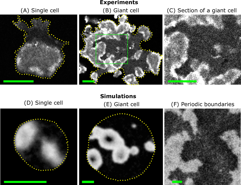
Figure 1. Actin waves in experiments (top) and model simulations (bottom). (A) Normal-sized cell with a circular actin wave. (B) Giant cell with several fragmented actin waves. (C) Subsection of the cortical area of the giant cell shown in (B), indicated as dotted green rectangle. Experimental images are confocal microscopy recordings of mRFP-LimE$\Delta$ expressing D. discoideum AX2 cells, see [GEW⁺14]. (Bottom) Simulations of the stochastic reaction-diffusion model (3), (4) in a (D) small and (E) large domain, defined by a dynamically evolving phase field and (F) with periodic boundary conditions. For details on the phase field simulations, see [FFAB20]. (Scale bars, 10 $\mathrm{\SIUnitSymbolMicro}$m) Details on the numerical implementation can be found in Appendix B.

Giant cells of NF1-deficient strains thus provide a well-suited setting to study the dynamics of actin waves and their impact on cell shape and division [FFAB20].

In Figure 1A and B, we show a normal-sized and a giant D. discoideum cell in the wave-forming regime for comparison. Images were recorded by confocal laser scanning microscopy and display the distribution of mRFP-LimE$\Delta$, a fluorescent marker for filamentous actin, in the cortex at the substrate-attached bottom membrane of the cell. As individual actin filaments are not resolved by this method, the intensity of the fluorescence signal reflects the local cortical density of filamentous actin. Rectangular subsections of the inner part of the cortex of giant cells as displayed in panel (C) were used for data analysis in Section 4.

Many aspects of subcellular dynamical patterns have been addressed by reaction-diffusion models. While some models rely on detailed modular approaches [BAB08, DBE⁺17], others have focused on specific parts of the upstream signaling pathways, such as the phosphatidylinositol lipid signaling system [ASM⁺10] or Ras signaling [FMU19]. To describe wave patterns in the actin cortex of giant D. discoideum cells, the noisy FitzHugh–Nagumo type reaction-diffusion system (3), (4), combined with a dynamic phase field, has been recently proposed [FFAB20]. In contrast to the more detailed biochemical models, the structure of this model is rather simple. Waves are generated by noisy bistable/excitable kinetics with an additional control of the total amount of activator $U$. This constraint dynamically regulates the amount of $U$ around a constant level in agreement with the corresponding biological restrictions. Elevated levels of the activator represent typical cell front markers, such as active Ras, PIP3, Arp2/3, and freshly polymerized actin that are also concentrated in the inner part of actin waves. On the other hand, markers of the cell back, such as PIP2, myosin II, and cortexillin, correspond to low values of $U$ and are found outside the wave area [SDGE⁺09]. Tuning of the parameter $b$ allows to continuously shift from bistable to excitable dynamics, both of which are observed in experiments with D. discoideum cells. In Figure 1D-F, the results of numerical simulations of this model displaying excitable dynamics are shown. Examples for bounded domains that correspond to normal-sized and giant cells are shown, as well as results with periodic boundary conditions that were used in the subsequent analysis.

Model parameters, such as the diffusivities, are typically chosen in an ad hoc fashion to match the speed of intracellular waves with the experimental observations. The approach introduced in Section 2 now allows us to estimate diffusivities from data in a more rigorous manner. On the one hand, we may test the validity of our method on in silico data of model simulations, where all parameters are predefined. On the other hand, we can apply our method to experimental data, such as the recordings of cortical actin waves displayed in Figure 1C. This will yield an estimate of the diffusivity of the activator $U$, as dense areas of filamentous actin reflect increased concentrations of activatory signaling components. Note, however, that the estimated value of $D_{U}$ should not be confused with the molecular diffusivity of a specific signaling molecule. It rather reflects an effective value that includes the diffusivities of many activatory species of the signaling network and is furthermore affected by the specific two-dimensional setting of the model that neither includes the kinetics of membrane attachment/detachment nor the three-dimensional cytosolic volume.

4. Diffusivity Estimation on
Simulated and Real Data

In this section we apply the methods from Section 2 to synthetic data obtained from a numerical simulation and to cell data stemming from experiments as described in Section 3. We follow the formalism from Theorem 5 and perform a Fourier decomposition on each data set. Set $\phi_{k}(x)=\cos(2\pi kx)$ for $k\leq 0$ and $\phi_{k}(x)=\sin(2\pi kx)$ for $k>0$, then $\Phi_{k,l}(x,y)=\phi_{k}(x/L_{1})\phi_{l}(y/L_{2})$, $k,l\in\mathbb{Z}$, form an eigenbasis for $-\Delta$ on the rectangular domain $\mathcal{D}=[0,L_{1}]\times[0,L_{2}]$. The corresponding eigenvalues are given by $\lambda_{k,l}=4\pi^{2}((k/L_{1})^{2}+(l/L_{2})^{2})$. As before, we choose an ordering $((k_{N},l_{N}))_{N\in\mathbb{N}}$ of the eigenvalues (excluding $\lambda_{0,0}=0$) such that $\lambda_{N}=\lambda_{k_{N},l_{N}}$ is increasing.

In the sequel, we will use different versions of $\hat{\theta}^{N}_{0}$ which correspond to different model assumptions on the reaction term $F$, concerning both the effects included in the model and a priori knowledge on the parametrization. While all of these estimators enjoy the same asymptotic properties as $N\rightarrow\infty$, it is reasonable to expect that they exhibit huge qualitative differences for fixed $N\in\mathbb{N}$, depending on how much knowledge on the generating dynamics is incorporated. In order to describe the model nonlinearities that we presume, we use the notation $F_{1},F_{2},F_{3}$ as in (10), (11), (12). As a first simplification, we substitute $F_{1}$ by $\widetilde{F}_{1}$ given by

(31) $$\widetilde{F}_{1}(U)=-U(u_{0}-U)$$

in all estimators below. This corresponds to an approximation of the function $a$ by an effective average value $\bar{a}>0$. While this clearly does not match the full model, we will see that it does not pose a severe restriction as $a(U)$ tends to stabilize in the simulation. Recall the explicit representation (21) of $\hat{\theta}^{N}_{0}$. As before, $K$ is the number of nuisance parameters appearing in the nonlinear term $F$. We construct the following estimators which capture qualitatively different model assumptions:

1. The linear estimator $\hat{\theta}^{\mathrm{lin},N}_{0}$ results from presuming $K=0$ and $F=0$.

2. The polynomial or Schlögl estimator $\hat{\theta}^{\mathrm{pol},N}_{0}$, where $K=0$ and

   $$F(u) =k_{1}u(u_{0}-u)(u-\bar{a}u_{0})$$

   $$=-k_{1}\bar{a}u_{0}u(u_{0}-u)+k_{1}u^{2}(u_{0}-u)$$

   $$=\theta_{1}\widetilde{F}_{1}(u)+\theta_{2}F_{2}(u)$$

   for known constants $k_{1},u_{0},\bar{a}>0$, $\theta_{1}=k_{1}u_{0}\bar{a}$, $\theta_{2}=k_{1}$. The corresponding SPDE (5) is called stochastic Nagumo equation or stochastic Schlögl equation and arises as the limiting case $\epsilon\rightarrow 0$ of the stochastic FitzHugh–Nagumo system.

3. The full or FitzHugh–Nagumo estimator $\hat{\theta}^{\mathrm{full},N}_{0}$, where $K=0$ and

   (32) $$\begin{matrix}[l]F(u)&=k_{1}u(u_{0}-u)(u-\bar{a}u_{0})-k_{2}v\\ &=\theta_{1}\widetilde{F}_{1}(u)+\theta_{2}F_{2}(u)+\theta_{2}F_{3}(u)\end{matrix}$$

   with $\theta_{1}=k_{1}u_{0}\bar{a}$, $\theta_{2}=k_{1}$ and $\theta_{3}=k_{2}\epsilon b$, where $v$ is given by $v_{t}=\int_{0}^{t}e^{(t-r)(D_{V}\Delta-\epsilon I)}u_{r}\mathrm{d}r$. As before, $k_{1},k_{2},u_{0},\bar{a},D_{v},\epsilon>0$ are known.

Furthermore, we modify $\hat{\theta}^{\mathrm{full},N}_{0}$ in order to estimate different subsets of model parameters at the same time. We use the notation $\hat{\theta}^{i,N}_{0}$, where $i$ is the number of simultaneously estimated parameters. More precisely, we set $\hat{\theta}^{1,N}_{0}=\hat{\theta}^{\mathrm{full},N}_{0}$, and additionally:

1. The estimator $\hat{\theta}^{2,N}_{0}$ results from $K=1$ and $F_{\theta_{1}}$ given by (32) for known $\theta_{2},\theta_{3}>0$. This corresponds to an unknown $\bar{a}$.

2. The estimator $\hat{\theta}^{3,N}_{0}$ results from $K=2$ and $F_{\theta_{1},\theta_{2}}$ given by (32). Only $\theta_{3}$ is known.

3. The estimator $\hat{\theta}^{4,N}_{0}$ results from $K=3$ and $F_{\theta_{1},\theta_{2},\theta_{3}}$ given by (32). All three parameters $\theta_{1},\theta_{2},\theta_{3}$ are unknown.

In all estimators in this section we set the regularity adjustment $\alpha=0$. This is a reasonable choice if the driving noise in (7), (8) is close to white noise.

It is worthwhile to note that $\hat{\theta}^{\mathrm{lin},N}_{0}$ is invariant under rescaling the intensity of the data, i.e. substituting $X$ by $cX$, $c>0$. This has the advantage that we do not need to know the physical units of the data. In fact, the intensity of fluorescence microscopy data may vary due to different expression levels of reporter proteins within a cell population, or fluctuations in the illumination. While invariance under intensity rescaling is a desirable property, the fact that nonlinear reaction terms are not taken into account may outweigh this advantage, especially if the SPDE model is close to the true generating process of the data. This is the case for synthetic data. The discussion in Section 4.1 shows that even if the model specific correction terms in (21) vanish asymptotically, their effect on the estimator may be huge in the non-asymptotic regime, especially at low resolution level. However, real data may behave differently, and a detailed nonlinear model may not reveal additional information on the underlying diffusivity, see Section 4.4.

4.1. Performance on Synthetic Data

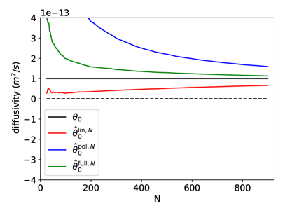
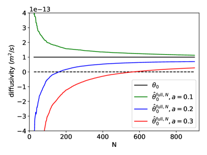
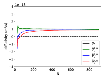
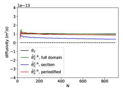
Figure 2. Performance of diffusivity estimators on simulated data under different model assumptions in the spatial high-frequency regime. Solid black line is plotted at the true parameter $\theta_{0}=1\times 10^{-13}$, dashed black line is plotted at zero. In all displays, we restrict to $N\geq 25$ in order to avoid artefacts stemming from low resolution.

First, we study the performance of the mentioned estimators on simulations. The numerical scheme is specified in Appendix B. While we have perfect knowledge on the dynamical system which generates the data in this setting, it is revelatory to compare the different versions of $\hat{\theta}^{N}_{0}$ which correspond to varying levels of model misspecification. The simulation shows that $a(|U_{t}|_{L^{2}})$ fluctuates around a value slightly larger than $0.15$. We demonstrate the effect of qualitatively different model assumptions on our method in Figure 2 (top left) by comparing the performance of $\hat{\theta}^{\mathrm{lin},N}_{0}$, $\hat{\theta}^{\mathrm{pol},N}_{0}$ and $\hat{\theta}^{\mathrm{full},N}_{0}$. The result can be interpreted as follows: As $\hat{\theta}^{\mathrm{lin},N}_{0}$ does not see any information on the wave fronts, the steep gradient at the transition phase leads to a low diffusivity estimate. On the other hand, $\hat{\theta}^{\mathrm{pol},N}_{0}$ incorporates knowledge on the wave fronts as they appear in the Schlögl model, but the decay in concentration due to the presence of the inhibitor is mistaken as additional diffusion. Finally, $\hat{\theta}^{\mathrm{full},N}_{0}$ contains sufficient information on the dynamics to give a precise estimate. In Figure 2 (top right), we show the effect of wrong a priori assumptions on $\bar{a}$ in $\hat{\theta}^{\mathrm{full},N}_{0}$. Even for $N=800$, the precision of $\hat{\theta}^{\mathrm{full},N}_{0}$ clearly depends on the choice of $\bar{a}$. Remember that there is no true $\bar{a}$ in the underlying model, rather, $\bar{a}$ serves as an approximation for $a(|U_{t}|_{L^{2}})$. Better results can be achieved with $\hat{\theta}^{2,N}_{0},\hat{\theta}^{3,N}_{0}$ and $\hat{\theta}^{4,N}_{0}$, see Figure 2 (bottom left): $\hat{\theta}^{2,N}_{0}$ has no knowledge on $\bar{a}$ and recovers the diffusivity precisely, and even $\hat{\theta}^{4,N}_{0}$ performs better than the misspecified $\hat{\theta}^{\mathrm{full},N}_{0}$ from the top right panel of Figure 2.

4.2. Discussion of the periodic boundary

In Figure 2 (bottom right) we sketch how the assumption of periodic boundary conditions influences the estimate. While $\hat{\theta}^{2,N}_{0}$ works very well on the full domain of $200\times 200$ pixels with periodic boundary conditions, it decays rapidly if we just use a square section of $75\times 75$ pixels. In fact, the boundary conditions are not satisfied on that square section. This leads to the presence of discontinuities at the boundary. These discontinuities, if interpreted as steep gradients, lower the observed diffusivity. Hence, a first guess to improve the quality is to mirror the square section along each axis and glue the results together. In this manner we construct a domain with $150\times 150$ pixels, on which $\hat{\theta}^{2,N}_{0}$ performs well. We emphasize that, while this periodification procedure is a natural approach, its performance will depend on the specific situation, because the dynamics at the transition edges will still not obey the true underlying dynamics. Furthermore, by modifying the data set as explained, we change its resolution, and consequently, a different amount of spectral information may be included into $\hat{\theta}^{2,N}_{0}$ for interpretable results.

4.3. Effect of the Noise Intensity

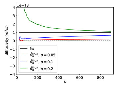
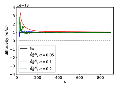
Figure 3. Sensitivity of (left) $\hat{\theta}^{\mathrm{lin},N}_{0}$ and (right) $\hat{\theta}^{2,N}_{0}$ to different noise levels. Solid black line is plotted at $\theta_{0}=1\times 10^{-13}$, dashed black line is plotted at zero. As before, we restrict to $N\geq 25$ in the plots.

In Figure 3, we study the effect of varying the noise level in the simulation. We compare $\hat{\theta}^{\mathrm{lin},N}_{0}$, which is agnostic to the reaction model, to $\hat{\theta}^{2,N}_{0}$, which incorporates a detailed reaction model. While $\hat{\theta}^{2,N}_{0}$ performs well regardless of the noise level, the quality of $\hat{\theta}^{\mathrm{lin},N}_{0}$ tends to improve for larger $\sigma$. In this sense, a large noise amplitude hides the effect of the nonlinearity. This is in line with the observations made in [PS20, Section 3]. We note that the dynamical features of the process change for $\sigma=0.2$: It is no longer capable of generating travelling waves in that case.

4.4. Performance on Real Data

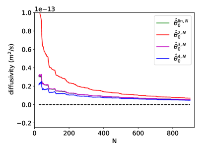
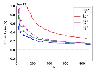
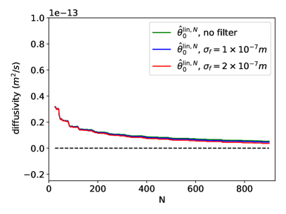
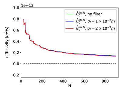
Figure 4. In all displays, we restrict to $N\geq 25$ in order to avoid artefacts stemming from low resolution. Dashed black line is plotted at zero. (top) Performance of different diffusivity estimators on (top left) cell data and (top right) periodified cell data. (bottom) The effects of applying a kernel with bandwidth $\bar{\sigma}$ is shown for (bottom left) not periodified and (bottom right) periodified data.

A description of the experimental setup can be found in Appendix B. The concentration in the data is represented by grey values ranging from $0$ to $255$ at every pixel. This range is standardized to the unit interval $[0,1]$, in order to match the stable fixed points of the bistable polynomial $f$ in the reference case $u_{0}=1$. Note that this is necessary for all estimators except $\hat{\theta}^{\mathrm{lin},N}_{0}$. We compare $\hat{\theta}^{\mathrm{lin},N}_{0}$ with $\hat{\theta}^{2,N}_{0}$, $\hat{\theta}^{3,N}_{0}$ and $\hat{\theta}^{4,N}_{0}$, which are more flexible than $\hat{\theta}^{\mathrm{pol},N}_{0}$ and $\hat{\theta}^{\mathrm{full},N}_{0}$. In Figure 4 (top left) the behaviour of these four estimators on a sample cell is shown. Interestingly, the model-free linear estimator $\hat{\theta}^{\mathrm{lin},N}_{0}$ is close to $\hat{\theta}^{3,N}_{0}$ and $\hat{\theta}^{4,N}_{0}$, which impose very specific model assumptions. This pattern can be observed across different cell data sets. In particular, this is notably different from the performance of these three estimators on synthetic data. This discrepancy seems to indicate that the lower order reaction terms in the activator-inhibitor model are not fully consistent with the information contained in the experimental data. This can have several reasons, for example, it is possible that a more detailed model reduction of the known signalling pathway inside the cell is needed. On the contrary, $\hat{\theta}^{2,N}_{0}$ seems to be comparatively rigid due to its a priori choices for $\theta_{2}$ and $\theta_{3}$, but it eventually approaches the other estimators. Variations in the value of $u_{0}$ have an impact on the results for small $N$ but not on the asymptotic behaviour. In Figure 4 (top right), the cell from Figure 4 (top left) is periodified before evaluating the estimators. As expected from the discussion in Section 4.2, the estimates rise, but the order of magnitude does not change drastically.

4.5. Invariance under Convolution

Given a function $k\in L^{1}(\mathcal{D})$, define $T_{k}:H^{s}(\mathcal{D})\rightarrow H^{s}(\mathcal{D})$, $s\in\mathbb{R}$, via $u\mapsto k*u=\int_{\mathcal{D}}k(\cdot-x)u(x)\mathrm{d}x$, where $k$ and $u$ are identified with their periodic continuation. It is well-known that $T_{k}$ commutes with $\Delta$, i.e. $T_{k}\circ\Delta=\Delta\circ T_{k}$. Thus, if $X$ is a solution to a semilinear stochastic PDE with diffusivity $\theta$, the same is true for $T_{k}X$: While the nonlinearity and the dispersion operator may be changed by $T_{k}$, the diffusive part is left invariant, in particular the diffusivity of $X$ and $T_{k}X$ is the same. Based on this observation, a comparison between the effective diffusivity of $X$ and $T_{k}X$ for different choices of $k$ may serve as an indicator if the assumption that a data set $X$ is generated by a semilinear SPDE (5) is reasonable in the first place, and if the diffusion indeed can be considered to be homogeneous and anisotropic. We use a family of periodic kernels $k=k_{\bar{\sigma}}$, $\bar{\sigma}>0$, which are normed in $L^{1}(\mathcal{D})$ and coincide on the reference rectangle $[-L_{1}/2,L_{1}/2]\times[-L_{2}/2,L_{2}/2]$ with a Gaussian density with standard deviation $\bar{\sigma}$. In Figure 4 (bottom), the effects of applying $T_{k_{\bar{\sigma}}}$ for different bandwidths $\bar{\sigma}$ are shown for one data set and its periodification. While the diffusivity of the data without periodification on the left-hand panel is slightly affected by the kernel, more precisely, its tendency to fall is enlarged, the graphs for the effective diffusivity of the periodified data are virtually indistinguishable. Periodification seems to be compatible with the expected invariance under convolution, even if the periodified data is not generated by a semilinear SPDE but instead by joining smaller patches of that form. In total, these observations are in accordance with the previous sections and suggest that the statistical analysis of the data based on a semilinear SPDE model is reasonable.

4.6. The Effective Diffusivity of a Cell Population

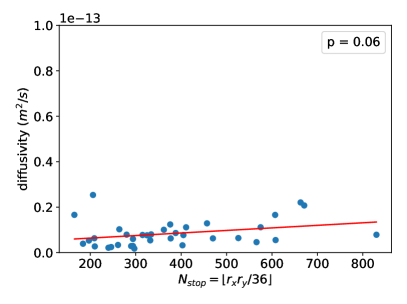
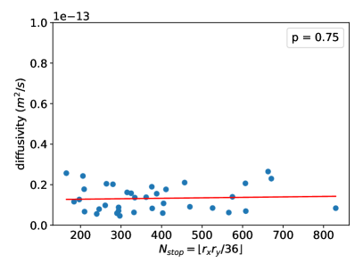
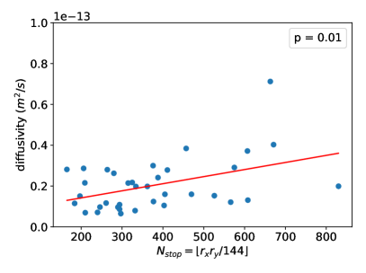
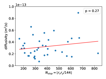
Figure 5. The samples are evaluated (top) without or (bottom) with periodification. $\hat{\theta}^{3,N}_{0}$ with (left) $N=N_{\mathrm{const}}$ or (right) $N=N_{\mathrm{stop}}$ is plotted against $N_{\mathrm{stop}}$. The least squares fit is shown in red. The $p$-value in each plot corresponds to a t-test whose null hypothesis states that the slope of the regression line is zero. Clearly, the slope is more notable in the case $N=N_{\mathrm{const}}$.

We compare the estimated diffusivity for a cell population consisting of $36$ cells. The boundaries in space and time of all samples are selected in order to capture only the interior dynamics within a cell and, consequently, the data sets differ in their size. On the one hand, the estimated diffusivity tends to stabilize in time, i.e. the number of frames in a sample, corresponding to the final time $T$, does not affect the result much. On the other hand, the size of each frame, measured in pixels, determines the number of eigenfrequencies that carry meaningful information on the process. Thus, we expect that $N$ can be chosen larger for samples with high spatial resolution. We formalize this intuition with the following heuristic: Let $r_{x}$ and $r_{y}$ denote the number of pixels in each row and column, resp., of every frame in a sample. Let $N_{\mathrm{stop}}=\lfloor 4r_{x}r_{y}/M^{2}\rfloor$, where $M\in\mathbb{N}$ is a parameter representing the number of pixels needed for a sine or cosine to extract meaningful information. That is, a square of dimensions $r_{x}\times r_{y}=M\times M$ leads to $N_{\mathrm{stop}}=4$, so in this case only the eigenfunctions $\Phi_{k,l}$, $k,l\in\{-1,1\}$ are taken into account, whose period length is $M$ in both dimensions. In our evaluations, we choose $M=12$ for the data without periodification and $M=24$ for the periodified data sets. We mention that the cells are also heterogeneous with respect to their characteristic length $\overline{dx}$ and time $\overline{dt}$, given in meters per pixel and seconds per frame for each data set. However, a detailed quantitative analysis of the resulting discretization error is beyond the scope of our work. In Figure 5, we compare the results for $\hat{\theta}^{3,N_{\mathrm{stop}}}_{0}$ with $\hat{\theta}^{3,N_{\mathrm{const}}}_{0}$ within the cell population, where $N_{\mathrm{const}}=899$ is independent of the sample resolution. Evaluating the estimator at $N_{\mathrm{stop}}$ decorrelates the estimated diffusivity from the spatial extension of the sample. The results for different cells have the same order of magnitude, which indicates that the effective diffusivity can be used for statistical inference for cells within a population or between populations in future research.

4.7. Estimating $\theta_{1}$.

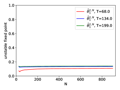
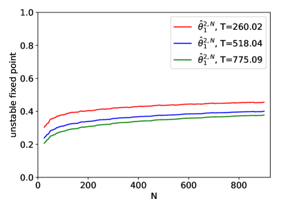
Figure 6. Estimation of the reaction parameter $\theta_{1}$ on (left) simulated data and (right) cell data. All times are given in seconds, relative to the first frame. As before, we restrict to $N\geq 25$.

When solving the linear MLE equations in order to obtain $\hat{\theta}^{2,N}_{0}$, we simultaneously get an estimate $\hat{\theta}_{1}^{2,N}$ for $\theta_{1}=k_{1}u_{0}\bar{a}$. Note that $u_{0}=1$ by convention, and $\theta_{2}=k_{1}=1$ is treated as known quantity in this case. Thus, $\theta_{1}$ can be identified with $\bar{a}$. In Figure 6 we show the results for $\hat{\theta}_{1}^{1,N}$ on simulated data (left) and on a cell data sample (right). Note that in general, we cannot expect to observe increased precision for $\hat{\theta}_{1}^{2,N}$ as $N$ grows, because the reaction term is of order zero. However, it is informative to consider also the large time regime $T\rightarrow\infty$, i.e. to include more and more frames to the estimation procedure. In the case of simulated data, $a$ oscillates around an average value close to $0.15$, which should be considered to be the ground truth for $\bar{a}$. This effective value $\bar{a}$ is recovered well, even for small $T$, with increasing precision as $T$ grows. Clearly, this depends heavily on the model assumptions. In the case of cell data, the results are rather stable. This indicates that it may be reasonable to use the concept of an “effective unstable fixed point $\bar{a}$ of the reaction dynamics, conditioned on the model assumptions included in $\hat{\theta}^{2,N}_{0}$”, when evaluating cell data statistically.

4.8. The Case of Pure Noise Outside the Cell

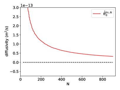
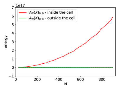
Figure 7. As before, we restrict to $N\geq 25$. (left) Effective diffusivity outside the cell, plot for one data set. Dashed line is plotted at zero. (right) Comparison of the energy inside and outside the cell. Both data sets have the same spatial and temporal extensions.

If the data set does not contain parts of the cell but rather mere noise, the estimation procedure still returns a value. This “observed diffusivity” (see Figure 7) originates completely from white measurement noise. More precisely, the appearance and vanishing of singular pixels is interpreted as instantaneous (i.e. within the time between two frames) diffusion to the steady state. Thus, the observed diffusivity in this case can be expected to be even larger than the diffusivity inside the cell. In this section, we give a heuristical explanation for the order of magnitude of the effective diffusivity outside the cell.

We work in dimension $d=2$. Assume that a pixel has width $x>0$. This value is determined by the spatial resolution of the data. For simplicity, we approximate it by a Gaussian density $\phi_{0}(y)$ with standard deviation $\sigma_{0}=\frac{x}{2}$. This way, the inflection points of the (one-dimensional marginal) density match the sharp edges of the pixel. Now, using $\phi_{0}$ as an initial condition for the heat equation on the whole space $\mathbb{R}^{2}$, the density $\phi_{t}$ after time $t$ is also a Gaussian density, with standard deviation $\sigma_{t}=\sqrt{\sigma_{0}^{2}+2\theta t}$, obtained by convolution with the heat kernel. The maximal value $f_{\mathrm{max}}^{t}$ of $\phi_{t}$ is attained at $y=0$ with $f_{\mathrm{max}}^{t}=(2\pi\sigma_{t}^{2})^{-1}=(2\pi(\sigma_{0}^{2}+2\theta t))^{-1}$. Now, if we observe after time $t>0$ at the given pixel an intensity decay by a factor $b>0$, i.e.

(33) $$bf_{\mathrm{max}}^{t}\leq f_{\mathrm{max}}^{0},$$

this leads to an estimate for the diffusivity of the form

(34) $$\theta\geq(b-1)\frac{\sigma_{0}^{2}}{2t}.$$

For example, set $t=0.97s$ and $x=2.08\times 10^{-7}m$, as in the data set from Figure 7 (left). The intensity decay factor varies between different pixels in the data set, reasonable values are given for $b\leq 30$. If $b=30$, we get $\theta\geq 1.6\times 10^{-13}m^{2}/s$, for $b=20$, we get $\theta\geq 1\times 10^{-13}m^{2}/s$, and for $b=15$, we have $\theta\geq 7.8\times 10^{-14}m^{2}/s$. This matches the observed diffusivity outside the cell from Figure 7, which is indeed of order $1\times 10^{-13}m^{2}/s$: For example, with $N=N_{\mathrm{stop}}=\lfloor 4r_{x}r_{y}/M^{2}\rfloor$ and $M=12$, as in Section 4.6, we get $N_{\mathrm{stop}}=165$ and $\hat{\theta}^{\mathrm{lin},N_{\mathrm{stop}}}_{0}=1.36\times 10^{-13}m^{2}/s$ for this data set consisting of pure noise. In total, this gives a heuristical explanation for the larger effective diffusivity outside the cell compared to the estimated values inside the cell.

It is important to note that even if the effective diffusivity outside the cell is larger, this has almost no effect on the estimation procedure inside the cell. This is because the total energy $A_{N}(X)_{0,0}$ of the noise outside the cell is several orders of magnitude smaller than the total energy of the signal inside the cell, see Figure 7 (right).

5. Discussion and Further Research

In this paper we have extended the mathematical theory of parameter estimation of stochastic reaction-diffusion system to the joint estimation problem of diffusivity and parametrized reaction terms within the variational theory of stochastic partial differential equations. We have in particular applied our theory to the estimation of effective diffusivity of intracellular actin cytoskeleton dynamics.

Traditionally, biochemical signaling pathways were studied in a purely temporal manner, focusing on the reaction kinetics of the individual components and the sequential order of the pathway, possibly including feedback loops. Relying on well-established biochemical methods, many of these temporal interaction networks could be characterized. However, with the recent progress in the in vivo expression of fluorescent probes and the development of advanced live cell imaging techniques, the research focus has increasingly shifted to studying the full spatiotemporal dynamics of signaling processes at the subcellular scale. To complement these experiments with modeling studies, stochastic reaction-diffusion systems are the natural candidate class of models that incorporate the relevant degrees of freedom of intracellular signaling processes. Many variants of this reaction-diffusion framework have been proposed in an empirical manner to account for the rich plethora of spatiotemporal signaling patterns that are observed in cells. However, the model parameters in such studies are oftentimes chosen in an ad hoc fashion and tuned based on visual inspection, so that the patterns produced in model simulations agree with the experimental observations. A rigorous framework that allows to estimate the parameters of stochastic reaction-diffusion systems from experimental data will provide an indispensable basis to refine existing models, to test how well they perform, and to eventually establish a new generation of more quantitative mathematical models of intracellular signaling patterns.

The question of robustness of the parameter estimation problem w.r.t. specific modelling assumptions of the underlying stochastic evolution equation is an important problem in applications that needs to be further investigated in future research. In particular, this applies to the dependence of diffusivity estimation on the domain and its boundary. In this work, we based our analysis on a Fourier decomposition on a rectangular domain with periodic boundary conditions. A natural, boundary-free approach is using local estimation techniques as they have been developed and used in [AR20, ACP20, ABJR20]. An additional approach aiming in the same direction is the application of a wavelet transform.

It is a crucial task to gather further information on the reaction term from the data. Principally, this cannot be achieved in a satisfactory way on a finite time horizon, so the long-time behaviour of maximum likelihood-based estimators needs to be studied in the context of stochastic reaction-diffusion systems. We will address this issue in detail in future work.

Appendix A Additional Proofs

A.1. Proof of Proposition 1

We prove Proposition 1 by a series of lemmas. First, we show that (7), (8) is well-posed in $\mathcal{H}=L^{2}\times L^{2}$. First note that for any $u,v\in L^{2}(\mathcal{D})$ and $x\in\mathbb{R}$:

(35) $$\langle\partial_{u}f(x,u)v,v\rangle_{L^{2}}\lesssim|v|_{L^{2}}^{2}$$

as $\partial f(x,u)$ is bounded from above uniformly in $x$ and $u$.

Lemma 8.

There is a unique $\mathcal{H}$-valued solution $(U,V)$ to (7), (8), and

(36) $$\mathbb{E}\left[\sup_{0\leq t\leq T}|(U_{t},V_{t})|_{\mathcal{H}}^{p}\right]<\infty$$

for any $p\geq 1$.

In particular,

(37) $$\mathbb{E}\left[\sup_{0\leq t\leq T}|U_{t}|_{L^{2}}^{p}\right]<\infty,\quad\mathbb{E}\left[\sup_{0\leq t\leq T}|V_{t}|_{L^{2}}^{p}\right]<\infty$$

for any $p\geq 1$.

Proof of Lemma 8.

This follows from [LR15, Theorem 5.1.3]. In order to apply this result, we have to test the conditions $(H1)$, $(H2^{\prime})$, $(H3)$, $(H4^{\prime})$ (i.e. hemicontinuity, local monotonicity, coercivity and growth) therein. Set $\mathcal{V}=H^{1}\times H^{1}$. Define $A(U,V)=(A_{1}(U,V),A_{2}(U,V))$ with

(38) $$A_{1}(U,V) =D_{U}\Delta U+k_{1}f(\lvert U\rvert_{L^{2}},U)-k_{2}V,$$

(39) $$A_{2}(U,V) =D_{V}\Delta V+\epsilon(bU-V).$$

As $B=(-\Delta)^{-\gamma}$ is constant and of Hilbert-Schmidt type, we can neglect it in the estimates. In order to check the conditions , we have to look separately at $A_{1}$ and $A_{2}$. The statements for $A_{2}$ is trivial by linearity, so we test the parts of the conditions corresponding to $A_{1}$. $(H1)$ is clear as $f(x,u)$ is a polynomial in $u$ and continuous in $x$. $(H2)$ follows from (35) via

$${}_{H^{-1}}\langle A_{1}(U_{1},V_{1})-A_{1}(U_{2},V_{2}),U_{1}-U_{2}\rangle_{H^{1}}$$

$$\lesssim k_{1}{}_{H^{-1}}\langle f(\lvert U_{1}\rvert_{L^{2}},U_{1})-f(\lvert U_{2}\rvert_{L^{2}},U_{2}),U_{1}-U_{2}\rangle_{H^{1}}$$

$$\quad+k_{2}|V_{1}-V_{2}|_{L^{2}}|U_{1}-U_{2}|_{L^{2}}$$

$$\lesssim k_{1}{}_{H^{-1}}\langle\partial_{u}f(\lvert U_{1}\rvert_{L^{2}}\widetilde{V})(U_{1}-U_{2}),U_{1}-U_{2}\rangle_{H^{1}}$$

$$\quad+k_{1}{}_{H^{-1}}\langle\partial_{x}f(\tilde{x},U_{2})(\lvert U_{1}\rvert_{L^{2}}-\lvert U_{2}\rvert_{L^{2}}),U_{1}-U_{2}\rangle_{H^{1}}$$

$$\quad+C\lVert(U_{1},V_{1})-(U_{2},V_{2})\rVert_{\mathcal{H}}^{2}$$

$$\lesssim k_{1}|\partial_{x}f(\tilde{x},U_{2})|_{L^{2}}\left|\lVert U_{1}\rVert_{L^{2}}-\lVert U_{2}\rVert_{L^{2}}\right||U_{1}-U_{2}|_{L^{2}}$$

$$\quad+C\lVert(U_{1},V_{1})-(U_{2},V_{2})\rVert_{\mathcal{H}}^{2}$$

$$\lesssim(1+|\partial_{x}f(\tilde{x},U_{2})|_{L^{2}})\lVert(U_{1},V_{1})-(U_{2},V_{2})\rVert_{\mathcal{H}}^{2}$$

for some $\tilde{x}\in\mathbb{R}$ and $\widetilde{V}:\mathcal{D}\rightarrow\mathbb{R}$, and $|\partial_{x}f(\tilde{x},U_{2})|_{L^{2}}=|u_{0}a^{\prime}(\tilde{x})U_{2}(u_{0}-U_{2})|_{L^{2}}\lesssim|U_{2}|_{L^{2}}+|U_{2}^{2}|_{L^{2}}$. With $|U_{2}^{2}|_{L^{2}}=|U_{2}|_{L^{4}}^{2}\lesssim|U_{2}|_{H^{1}}^{2}$, we see that local monotonicity as in $(H2)$ is satisfied by taking $\rho((u,v))=c|u|_{H^{1}}^{2}\leq c|(u,v)|_{\mathcal{V}}^{2}$. Now, for $(H3)$,

$${}_{H^{-1}}\langle A_{1}(U,V),U\rangle_{H^{1}} \leq-D_{U}|U|_{H^{1}}^{2}+k_{1}{}_{H^{-1}}\langle f(\lvert U\rvert_{L^{2}},U),U\rangle_{H^{1}}$$

$$\quad+k_{2}|U|_{L^{2}}|V|_{L^{2}}$$

$$\lesssim-D_{U}|U|_{H^{1}}^{2}+k_{1}\langle\partial_{u}f(\lvert U\rvert_{L^{2}},\widetilde{V})U,U\rangle_{L^{2}}$$

$$\quad+C\lVert(U,V)\rVert_{\mathcal{H}}^{2}$$

$$\lesssim-D_{U}|U|_{H^{1}}^{2}+C|U|_{L^{2}}^{2}+C\lVert(U,V)\rVert_{\mathcal{H}}^{2}$$

for some $\widetilde{V}:\mathcal{D}\rightarrow\mathbb{R}$, again using (35). Finally,

$$\lvert A_{1}(U)\rvert_{H^{-1}}^{2} \lesssim D_{U}|U|_{H^{1}}^{2}+k_{1}|f(\lvert U\rvert_{L^{2}},U)|_{H^{-1}}^{2}+k_{2}|V|_{L^{2}}^{2},$$

so it remains to control $|f(\lvert U\rvert_{L^{2}},U)|_{H^{-1}}^{2}\lesssim|f(\lvert U\rvert_{L^{2}},U)|_{L^{1}}^{2}\lesssim|U|_{L^{1}}^{2}+|U^{2}|_{L^{1}}^{2}+|U^{3}|_{L^{1}}^{2}$, and we have $|U|_{L^{1}}^{2}\lesssim|U|_{L^{2}}^{2}$ as well as $|U^{2}|_{L^{1}}^{2}=|U|_{L^{2}}^{4}$ and $|U^{3}|_{L^{1}}^{2}=|U|_{L^{3}}^{6}\lesssim|U|_{H^{1/3}}^{6}\lesssim|U|_{H^{1}}^{2}|U|_{L^{2}}^{4}$. Thus $(H4)$ is true. Putting things together, we get that [LR15] is applicable for sufficiently large $p\geq 1$, and the claim follows. ∎

In order to improve (37) to the $H^{1}$-norm, it suffices to prove coercivity, i.e. $(H3)$ from [LR15], for the Gelfand triple $L^{2}\subset H^{1}\subset H^{2}$.

Lemma 9.

The solution $(U,V)$ to (7), (8) satisfies $(A_{1})$, i.e. for any $p\geq 1$:

(40) $$\mathbb{E}\left[\sup_{0\leq t\leq T}|U_{t}|_{H^{1}}^{p}\right]<\infty,\quad\mathbb{E}\left[\sup_{0\leq t\leq T}|V_{t}|_{H^{1}}^{p}\right]<\infty.$$

Proof.

This is done by

$${}_{L^{2}}\langle A_{1}(U,V),U\rangle_{H^{2}} \leq-D_{U}|U|_{H^{2}}^{2}+k_{1}\langle\partial_{u}f(\lvert U\rvert_{L^{2}},U)\nabla U,\nabla U\rangle_{L^{2}}$$

$$\quad+k_{2}|U|_{H^{1}}|V|_{H^{1}}$$

$$\lesssim-D_{U}|U|_{H^{2}}^{2}+C|U|_{H^{1}}^{2}+C\lVert(U,V)\rVert_{H^{1}\times H^{1}}^{2},$$

where (35) has been used componentwise. By [LR15, Lemma 5.1.5] we immediately obtain (40). ∎

Remember that by integrating (8), we can write (7) as

(41) $$\mathrm{d}U_{t}=(D_{U}\Delta U_{t}+\theta_{1}F_{1}(U_{t})+\theta_{2}F_{2}(U_{t})+\theta_{3}F_{3}(U)(t))\mathrm{d}t+B\mathrm{d}W_{t},$$

where we adopted the notation from (10), (11), (12).

Lemma 10.

The process $(U,V)$ satisfies $(A_{s})$ for some $s>1$.

Proof.

Let $U=\overline{U}+\widetilde{U}$ be the decomposition of $U$ into its linear and nonlinear part as in (14),(15). We will prove

(42) $$\mathbb{E}\left[\sup_{0\leq t\leq T}|\widetilde{U}_{t}|_{W^{s,q}}^{p}\right]<\infty$$

for any $p,q\geq 1$ and $s<2$. As $\gamma>d/4$ in $d\leq 2$, there is $s>1$ such that (42) is true for $\overline{U}$ with $q=2$, and the claim follows. Let us now prove (42). First, note that by Lemma 9 and the Sobolev embedding theorem in dimension $d\leq 2$, (42) is true for $U_{t}$ with any $p,q\geq 1$ and $s=0$. For $k\in\mathbb{N}$, by $|U_{t}^{k}|_{L^{q}}^{p}=|U_{t}|_{L^{kq}}^{kp}$, we see that polynomials in $U$ satisfy (42) with $s=0$, too. In particular, using that $a$ is bounded,

(43) $$\mathbb{E}\left[\sup_{0\leq t\leq T}|F_{i}(U_{t})|_{L^{q}}^{p}\right]<\infty$$

for $i=1,2$ and $p,q\geq 1$. A simple calculation shows that the same is true for $F_{3}$. As in the proof of Proposition 3, we see that

$$\sup_{0\leq t\leq T}|\widetilde{U}_{t}|_{\eta,q}\leq|U_{0}|_{\eta,q}+\frac{2}{\epsilon}T^{\frac{\epsilon}{2}}\sup_{0\leq t\leq T}|\theta_{1}F_{1}(U)+\theta_{2}F_{2}(U)+\theta_{3}F_{3}(U)|_{L^{q}}$$

with $\eta<2$, $q\geq 1$ and $\epsilon=2-\eta$, and the proof is complete. ∎

Proof of Proposition 1.

In $d\leq 2$, $H^{s}$ is an algebra for $s>1$, i.e. $uv\in H^{s}$ for $u,v\in H^{s}$ [AF03]. Together with the assumption that $a$ is bounded, it follows immediately that $(F_{s,\eta})$ holds for $F_{1}$, $F_{2}$ separately (with $K=0$) for any $s>1$ and $\eta<2$. For $F_{3}$, we have for any $\delta>0$:

(44) $$\sup_{0\leq t\leq T}|F_{3}(U_{t})|_{s+2-\delta} \leq\int_{0}^{T}|e^{(t-r)(D_{V}\Delta-\epsilon I)}U_{r}|_{s+2-\delta}\mathrm{d}r$$

(45) $$\leq\int_{0}^{T}(t-r)^{-1+\delta/2}|U_{r}|_{s}\mathrm{d}r$$

(46) $$\leq\frac{2}{\delta}T^{\frac{\delta}{2}}\sup_{0\leq t\leq T}|U_{t}|_{s},$$

so $F_{3}$ satisfies $(F_{s,\eta})$ even with $s\in\mathbb{R}$, $\eta<4$. It is now clear that the $(F_{s,\eta})$ holds for $F=\theta_{1}F_{1}+\theta_{2}F_{2}+\theta_{3}F_{3}$ for any $s>1$ and $\eta<2$ (with $K=3$). The claim follows from Proposition 3 (i) for $U$ and (ii) for $V$, noting that $V=\epsilon bF_{3}(U)$. ∎

A.2. Proof of Proposition 6

This section is devoted to proving Proposition 6. A similar argument can be found in [Hue93, Chapter 3] for linear SPDEs. We start with an auxiliary statement, which characterizes the rate of $\det(A_{N}(X))$. For simplicity of notation, we abbreviate $a^{N}_{i}:=A_{N}(X)_{i,i}$ for $i=0,\dots,K$. While there is a trival upper bound $\det(A_{N}(X))\lesssim a^{N}_{0}\dots a^{N}_{K}$ obtained by the Cauchy-Schwarz inequality, the corresponding lower bound requires more work. Our argument is geometric in nature: A Gramian matrix measures the (squared) volume of a parallelepiped spanned by the vectors defining the matrix. The argument takes place in the separable Hilbert space $L^{2}(0,T;H^{2\alpha})$, and we find a (uniform in $N$) lower bound on the $(K+1)$-dimensional volume of the parallelepiped spanned by the vectors $P_{N}(-\Delta)X,P_{N}F_{1}(X),\dots,P_{N}F_{K}(X)$. While the latter $K$ components (and thus their $K$-dimensional volume) converge, the first component gets eventually orthogonal to the others as $N$ grows. This is formalized as follows:

Lemma 11.

Let $\eta,s_{0}>0$ such that $(A_{s})$ and $(F_{s,\eta})$ are true for $s_{0}\leq s<2\gamma+1-d/2$. Let $\gamma-d/4-1/2<\alpha\leq\gamma-d/4-1/2+\eta/2$. Under assumption $(L_{\alpha})$, we have

(47) $$\det(A_{N}(X))\gtrsim a^{N}_{0}\dots a^{N}_{K}.$$

In particular, $A_{N}(X)$ is invertible if $N$ is large enough.

Proof.

The argument is pathwise, so we fix a realization of $X$. We abbreviate $\langle\cdot,\cdot\rangle_{\alpha}:=\langle\cdot,\cdot\rangle_{L^{2}(0,T;H^{2\alpha})}$ and $\lVert\cdot\rVert_{\alpha}:=|\cdot|_{L^{2}(0,T;H^{2\alpha})}$, further we write $F_{0}(X)=\Delta X$ in order to unify notation. By a simple normalization procedure, it suffices to show that

(48) $$\liminf_{N\rightarrow\infty}\det\left(\left(\left\langle\frac{P_{N}F_{i}(X)}{\lVert P_{N}F_{i}(X)\rVert_{\alpha}},\frac{P_{N}F_{j}(X)}{\lVert P_{N}F_{j}(X)\rVert_{\alpha}}\right\rangle_{\alpha}\right)_{i,j=0,\dots K}\right)>0.$$

Let $\epsilon>0$ and choose $N_{0},N_{1}\in\mathbb{N}$ with $N_{0}\leq N_{1}$ such that:

• $\lVert P_{N}F_{i}(X)-F_{i}(X)\rVert_{\alpha}<\epsilon\lVert F_{i}(X)\rVert_{\alpha}$ and $\lVert F_{i}(X)\rVert_{\alpha}/\lVert P_{N}F_{i}(X)\rVert_{\alpha}<2$ for $i=1,\dots,K$ and $N\geq N_{0}$. This is possible due to $\alpha\leq\gamma-d/4-1/2+\eta/2.$

• $\lVert P_{N_{0}}F_{0}(X)\,/\,\lVert P_{N}F_{0}(X)\rVert_{\alpha}\,\rVert_{\alpha}<\epsilon$ for $N\geq N_{1}$. This is possible as $\lVert P_{N}F_{0}(X)\rVert_{\alpha}$ diverges due to $\alpha>\gamma-d/4-1/2$.

Now one performs a Laplace expansion of (48) in the first column. Each entry of the matrix in (48) can be bounded by $1$ trivially, but we can say more:

$$\left|\left\langle\frac{P_{N}F_{0}(X)}{\lVert P_{N}F_{0}(X)\rVert_{\alpha}},\frac{P_{N}F_{i}(X)}{\lVert P_{N}F_{i}(X)\rVert_{\alpha}}\right\rangle_{\alpha}\right| \leq\left|\left\langle\frac{P_{N_{0}}F_{0}(X)}{\lVert P_{N}F_{0}(X)\rVert_{\alpha}},\frac{P_{N_{0}}F_{i}(X)}{\lVert P_{N}F_{i}(X)\rVert_{\alpha}}\right\rangle_{\alpha}\right|$$

$$\quad+\left|\left\langle\frac{(P_{N}-P_{N_{0}})F_{0}(X)}{\lVert P_{N}F_{0}(X)\rVert_{\alpha}},\frac{(P_{N}-P_{N_{0}})F_{i}(X)}{\lVert P_{N}F_{i}(X)\rVert_{\alpha}}\right\rangle_{\alpha}\right|$$

$$\leq\left\lVert\frac{P_{N_{0}}F_{0}(X)}{\lVert P_{N}F_{0}(X)\rVert_{\alpha}}\right\rVert_{\alpha}+\left\lVert\frac{(I-P_{N_{0}})F_{i}(X)}{\lVert P_{N}F_{i}(X)\rVert_{\alpha}}\right\rVert_{\alpha}$$

$$\leq\epsilon+2\epsilon$$

for $N\geq N_{1}$ with $i=1,\dots,K$, where we used the Cauchy-Schwarz inequality and the choice of $N_{0}$, $N_{1}$. Consequently, in order for (48) to be true, it suffices to show for the $(0,0)$-minor:

(49) $$\liminf_{N\rightarrow\infty}\det\left(\left(\left\langle\frac{P_{N}F_{i}(X)}{\lVert P_{N}F_{i}(X)\rVert_{\alpha}},\frac{P_{N}F_{j}(X)}{\lVert P_{N}F_{j}(X)\rVert_{\alpha}}\right\rangle\right)_{i,j=1,\dots K}\right)>0.$$

By $(L_{\alpha})$, we have

(50) $$\det\left(\left(\left\langle\frac{F_{i}(X)}{\lVert F_{i}(X)\rVert_{\alpha}},\frac{F_{j}(X)}{\lVert F_{j}(X)\rVert_{\alpha}}\right\rangle_{\alpha}\right)_{i,j=1,\dots K}\right)>0,$$

so (49) holds true by continuity for $i=1,\dots,K$. ∎

Proof of Proposition 6.

As before, we formally write $F_{0}(X)=\Delta X$ in order to unify notation. By plugging in the dynamics of $X$, we see that for $i=0,\dots,K$,

(51) $$b_{N}(X)_{i}=\int_{0}^{T}\langle(-\Delta)^{2\alpha-\gamma}P_{N}F_{i}(X),\mathrm{d}W^{N}_{t}\rangle+\sum_{k=0}^{K}\theta_{k}A_{N}(X)_{i,k}.$$

Thus, with $\bar{b}_{N}(X)_{i}=\int_{0}^{T}\langle(-\Delta)^{2\alpha-\gamma}P_{N}F_{i}(X),\mathrm{d}W^{N}_{t}\rangle$ and $\theta=(\theta_{0},\dots,\theta_{K})^{T}$, this read as

(52) $$A_{N}(X)\hat{\theta}^{N}(X)=\bar{b}_{N}(X)+A_{N}(X)\theta,$$

i.e.

(53) $$\hat{\theta}^{N}-\theta=A_{N}^{-1}(X)\bar{b}_{N}(X).$$

Using the explicit representation for the inverse matrix $A_{N}(X)^{-1}$, we have

(54) $$\hat{\theta}^{N}_{j}-\theta_{j}=\frac{1}{\det(A_{N}(X))}\sum_{i=0}^{K}(-1)^{i+j}\det(\overline{A}^{(i,j)}_{N}(X))\bar{b}_{N}(X)_{i},$$

where $\overline{A}^{(i,j)}_{N}(X)$ results from $A_{N}(X)$ by erasing the $i$th row and the $j$th column. Remember that by Lemma 4, $a^{N}_{0}\asymp C_{\alpha}N^{\frac{2}{d}(2\alpha-2\gamma+1)+1}$. Further, due to $\alpha\leq\gamma-d/4-1/2+\eta/2$, $a^{N}_{i}/a^{N}_{0}\rightarrow 0$ in probability for all $i=1,\dots,K$. Now, by the Cauchy-Schwarz inequality, each summand in the numerator can be bounded by terms of the form

(55) $$\prod_{k=0}^{K}a^{N}_{k}\frac{|\bar{b}_{N}(X)_{i}|}{\sqrt{a^{N}_{i}a^{N}_{j}}}$$

for $i,j=0,\dots,K$. Thus, by Lemma 11, in order to prove the claim it remains to find a uniform bound in probability for the terms of the form $|\bar{b}_{N}(X)_{i}|/\sqrt{a^{N}_{i}a^{N}_{j}}$. Now, for $i=1,\dots,K$,

(56) $$\mathbb{E}{\left[\bar{b}_{N}(X)_{i}^{2}\right]} =\mathbb{E}\left[\left(\int_{0}^{T}\langle(-\Delta)^{2\alpha-\gamma}P_{N}F_{i}(X),\mathrm{d}W^{N}_{t}\rangle\right)^{2}\right]$$

(57) $$=\mathbb{E}\left[\int_{0}^{T}|(-\Delta)^{2\alpha-\gamma}P_{N}F_{i}(X)|_{H}^{2}\mathrm{d}t\right]<\infty$$

uniformly in $N$ as $\alpha<\gamma-d/8-1/4+\eta/4$. Further, $(a^{N}_{0})^{-1/2}$ converges to zero in probability, while $(a^{N}_{i})^{-1/2}$ converges to a positive constant for $i=1,\dots,K$. For $i=0$, the reasoning is similar: By Propositon 3 and Lemma 4, we have

(58) $$\mathbb{E}\left[\bar{b}_{N}(X)_{0}^{2}\right]\asymp\mathbb{E}\left[\int_{0}^{T}|(-\Delta)^{1+2\alpha-\gamma}\overline{X}^{N}_{t}|_{H}^{2}\mathrm{d}t\right]\asymp C_{2\alpha-\gamma}N^{\frac{2}{d}(4\alpha-4\gamma+1)+1}.$$

Together with $a_{0}^{N}\sim N^{\frac{2}{d}(2\alpha-2\gamma+1)+1}$ and $\alpha\leq\gamma$, this yields that $\bar{b}_{N}(X)_{0}^{2}/a^{N}_{0}$ (and consequently $|\bar{b}_{N}(X)_{0}|/\sqrt{a^{N}_{0}a^{N}_{j}}$ for $j=0,\dots,K$) is bounded in probability. The claim follows. ∎

Appendix B Methods

Numerical simulation

For the evaluation in Section 4 and Figure 1 (F) we simulated (7), (8) on a square with side $L=75$, with spatial increment $\mathrm{d}x=0.375$, for $t\in[T_{0},T_{1})$, $T_{0}=500$, $T_{1}=700$, with temporal increment $\mathrm{d}t=0.01$, using an explicit finite difference scheme, of which we recorded every $100$th frame. We choose $T_{0}=500$ in order to avoid artefacts stemming from zero initial conditions at $T=0$. We set $b=0.2$, $\gamma=0$, $\sigma=0.1$ and $a(x)=0.5-b+0.5(x/(0.33u_{0}L^{2})-1)$. In Section 4.3, we use additional simulations with $\sigma=0.05$ and $\sigma=0.2$.

For single and giant cell simulations in Figure 1 (D), (E) we solve (7), (8) on a square with side $L=75$, with spatial increment $\mathrm{d}x=0.15$, for $t\in[0,T]$, $T=1000$, with temporal increment $\mathrm{d}t=0.002$, using an explicit finite difference scheme together with a phase field model [FFAB20] to account for the interior of the single and giant cells, corresponding, respectively, to an area of A₀=113 $\mathrm{\SIUnitSymbolMicro}$$m^{2}$ and A₀=2290 $\mathrm{\SIUnitSymbolMicro}$$m^{2}$. We used $b=0.4$ and $a(x)=0.5-b+0.5(x/(0.25u_{0}A_{0})-1)$. The noise terms are chosen as in [FFAB20], with $\sigma=0.1$ and $k_{\eta}=0.1$ in the notation therein.

For both simulations, the remaining parameters are $D_{U}=0.1,D_{V}=0.02,k_{1}=k_{2}=1,u_{0}=1,\epsilon=0.02$. The unit length is 1 $\mathrm{\SIUnitSymbolMicro}$m, the unit time is $1s$.

Experimental settings

For experiments D. discoideum AX2 cells expressing mRFP-LimE$\Delta$ as a marker for F-actin were used. Cell culture and electric pulse induced fusion to create giant cells were performed as described in [GEW⁺14, FFAB20]. For live cell imaging an LSM 780 (Zeiss, Jena) with a 63x objective lens (alpha Plan-Apochromat, NA 1.46, Oil Korr M27, Zeiss Germany) were used. The spatial and temporal resolution was adjusted for each individual experiment to acquire image series with the best possible resolution, while protecting the cells from photo damage. Images series were saved as 8-bit tiff files. For image series where the full range of 256 pixel values was not utilized, the image histograms were optimized in such a way that the brightest pixels corresponded to a pixel value of 255.

References

• [ABJR20] R. Altmeyer, T. Bretschneider, J. Janák, and M. Reiß, Parameter Estimation in an SPDE Model for Cell Repolarization, Preprint: arXiv:2010.06340 [math.ST], 2020.
• [ACP20] R. Altmeyer, I. Cialenco, and G Pasemann, Parameter Estimation for Semilinear SPDEs from Local Measurements, Preprint: arXiv:2004.14728 [math.ST], 2020.
• [AF03] R. A. Adams and J. J. F. Fournier, Sobolev Spaces, second ed., Pure and Applied Mathematics, vol. 140, Elsevier/Academic Press, 2003.
• [AF09] Sarah J. Annesley and Paul R. Fisher, Dictyostelium discoideum—a model for many reasons, Molecular and Cellular Biochemistry 329 (2009), no. 1-2, 73–91.
• [AR20] R. Altmeyer and M. Reiß, Nonparametric Estimation for Linear SPDEs from Local Measurements, Annals of Applied Probability (2020), to appear.
• [ASB18] Sergio Alonso, Maike Stange, and Carsten Beta, Modeling random crawling, membrane deformation and intracellular polarity of motile amoeboid cells, PLOS ONE 13 (2018), no. 8, e0201977.
• [ASM+10] Yoshiyuki Arai, Tatsuo Shibata, Satomi Matsuoka, Masayuki J. Sato, Toshio Yanagida, and Masahiro Ueda, Self-organization of the phosphatidylinositol lipids signaling system for random cell migration, Proceedings of the National Academy of Sciences 107 (2010), no. 27, 12399–12404.
• [BAB08] Carsten Beta, Gabriel Amselem, and Eberhard Bodenschatz, A bistable mechanism for directional sensing, New Journal of Physics 10 (2008), no. 8, 083015.
• [BBPSP14] Laurent Blanchoin, Rajaa Boujemaa-Paterski, Cécile Sykes, and Julie Plastino, Actin Dynamics, Architecture, and Mechanics in Cell Motility, Physiological Reviews 94 (2014), no. 1, 235–263.
• [BK17] Carsten Beta and Karsten Kruse, Intracellular Oscillations and Waves, Annual Review of Condensed Matter Physics 8 (2017), no. 1, 239–264.
• [BT19] M. Bibinger and M. Trabs, On central limit theorems for power variations of the solution to the stochastic heat equation, Stochastic Models, Statistics and Their Applications (A. Steland, E. Rafajłowicz, and O. Okhrin, eds.), Springer Proceedings in Mathematics and Statistics, vol. 294, Springer, 2019, pp. 69–84.
• [BT20] by same author, Volatility Estimation for Stochastic PDEs Using High-Frequency Observations, Stochastic Processes and their Applications 130 (2020), no. 5, 3005–3052.
• [CDVK20] I. Cialenco, F. Delgado-Vences, and H.-J. Kim, Drift Estimation for Discretely Sampled SPDEs, Stochastics and Partial Differential Equations: Analysis and Computations (2020), to appear.
• [CGH11] I. Cialenco and N. Glatt-Holtz, Parameter estimation for the stochastically perturbed Navier-Stokes equations, Stochastic Process. Appl. 121 (2011), no. 4, 701–724.
• [CH19] I. Cialenco and Y. Huang, A Note on Parameter Estimation for Discretely Sampled SPDEs, Stochastics and Dynamics (2019), doi:10.1142/S0219493720500161, to appear.
• [Cho19a] C. Chong, High-Frequency Analysis of Parabolic Stochastic PDEs, Annals of Statistics (2019), to appear.
• [Cho19b] by same author, High-Frequency Analysis of Parabolic Stochastic PDEs with Multiplicative Noise: Part I, Preprint: arXiv:1908.04145 [math.PR], 2019.
• [Cia10] Igor Cialenco, Parameter estimation for SPDEs with multiplicative fractional noise, Stoch. Dyn. 10 (2010), no. 4, 561–576.
• [Cia18] I. Cialenco, Statistical inference for SPDEs: an overview, Stat. Inference Stoch. Process. 21 (2018), no. 2, 309–329.
• [CK20] I. Cialenco and H.-J. Kim, Parameter estimation for discretely sampled stochastic heat equation driven by space-only noise revised, Preprint: arXiv:2003.08920 [math.PR], 2020.
• [CL09] Igor Cialenco and Sergey V. Lototsky, Parameter estimation in diagonalizable bilinear stochastic parabolic equations, Stat. Inference Stoch. Process. 12 (2009), no. 3, 203–219.
• [CSS05] John Condeelis, Robert H. Singer, and Jeffrey E. Segall, THE GREAT ESCAPE: When Cancer Cells Hijack the Genes for Chemotaxis and Motility, Annual Review of Cell and Developmental Biology 21 (2005), no. 1, 695–718.
• [DBE+17] Peter N. Devreotes, Sayak Bhattacharya, Marc Edwards, Pablo A. Iglesias, Thomas Lampert, and Yuchuan Miao, Excitable Signal Transduction Networks in Directed Cell Migration, Annual Review of Cell and Developmental Biology 33 (2017), no. 1, 103–125.
• [DPZ14] G. Da Prato and J. Zabczyk, Stochastic Equations in Infinite Dimensions, second ed., Encyclopedia of Mathematics and its Applications, vol. 152, Cambridge University Press, 2014.
• [ET10] G. Bard Ermentrout and David H. Terman, Mathematical foundations of neuroscience, Interdisciplinary Applied Mathematics, vol. 35, Springer, New York, 2010.
• [FFAB20] Sven Flemming, Francesc Font, Sergio Alonso, and Carsten Beta, How cortical waves drive fission of motile cells, Proceedings of the National Academy of Sciences 117 (2020), no. 12, 6330–6338.
• [Fit61] R. Fitzhugh, Impulses and Physiological States in Theoretical Models of Nerve Membrane, Biophys. J. 1 (1961), 445–466.
• [FMU19] Seiya Fukushima, Satomi Matsuoka, and Masahiro Ueda, Excitable dynamics of Ras triggers spontaneous symmetry breaking of PIP3 signaling in motile cells, Journal of Cell Science (2019), 12.
• [GEW+14] Matthias Gerhardt, Mary Ecke, Michael Walz, Andreas Stengl, Carsten Beta, and Günther Gerisch, Actin and PIP3 waves in giant cells reveal the inherent length scale of an excited state, J Cell Sci 127 (2014), no. 20, 4507–4517.
• [HKR93] M. Hübner, R. Khasminskii, and B. L. Rozovskii, Two Examples of Parameter Estimation for Stochastic Partial Differential Equations, Stochastic processes (S. Cambanis, J. K. Ghosh, R. L. Karandikar, and P. K. Sen, eds.), Springer, New York, 1993, pp. 149–160.
• [HLR97] M. Huebner, S. Lototsky, and B. L. Rozovskii, Asymptotic Properties of an Approximate Maximum Likelihood Estimator for Stochastic PDEs, Statistics and Control of Stochastic Processes (Y. M. Kabanov, B. L. Rozovskii, and A. N. Shiryaev, eds.), World Sci. Publ., 1997, pp. 139–155.
• [HR95] M. Huebner and B. L. Rozovskii, On asymptotic properties of maximum likelihood estimators for parabolic stochastic PDE’s, Probab. Theory Related Fields 103 (1995), no. 2, 143–163.
• [Hue93] M. Huebner, Parameter Estimation for Stochastic Differential Equations, ProQuest LLC, Ann Arbor, 1993, Thesis (Ph.D.)–University of Southern California.
• [JS03] J. Jacod and A. N. Shiryaev, Limit Theorems for Stochastic Processes, second ed., Grundlehren der Mathematischen Wissenschaften, vol. 288, Springer-Verlag, Berlin, Heidelberg, 2003.
• [KT19] Z. M. Khalil and C. Tudor, Estimation of the drift parameter for the fractional stochastic heat equation via power variation, Modern Stochastics: Theory and Applications 6 (2019), no. 4, 397–417.
• [KU19] Y. Kaino and M. Uchida, Parametric estimation for a parabolic linear spde model based on sampled data, Preprint: arXiv:1909.13557 [math.ST], 2019.
• [Lot03] S. Lototsky, Parameter Estimation for Stochastic Parabolic Equations: Asymptotic Properties of a Two-Dimensional Projection-Based Estimator, Stat. Inference Stoch. Process. 6 (2003), no. 1, 65–87.
• [LR99] S. V. Lototsky and B. L. Rosovskii, Spectral asymptotics of some functionals arising in statistical inference for SPDEs, Stochastic Process. Appl. 79 (1999), no. 1, 69–94.
• [LR00] S. Lototsky and B. L. Rozovskii, Parameter Estimation for Stochastic Evolution Equations with Non-Commuting Operators, Skorokhod’s ideas in probability theory (V. Korolyuk, N. Portenko, and H. Syta, eds.), Institute of Mathematics of the National Academy of Science of Ukraine, Kiev, 2000, pp. 271–280.
• [LR15] W. Liu and M. Röckner, Stochastic Partial Differential Equations: An Introduction, Universitext, Springer, 2015.
• [LS77] R. S. Liptser and A. N. Shiryayev, Statistics of Random Processes I (General Theory), Applications of Mathematics, vol. 5, Springer-Verlag, New York, 1977.
• [LS89] R. Sh. Liptser and A. N. Shiryayev, Theory of Martingales, Mathematics and its Applications (Soviet Series), vol. 49, Kluwer Academic Publishers Group, Dordrecht, 1989.
• [MFF+20] Eduardo Moreno, Sven Flemming, Francesc Font, Matthias Holschneider, Carsten Beta, and Sergio Alonso, Modeling cell crawling strategies with a bistable model: From amoeboid to fan-shaped cell motion, Physica D: Nonlinear Phenomena 412 (2020), 132591 (en).
• [NAY62] A. Nagumo, S. Arimoto, and S. Yoshizawa, An Active Pulse Transmission Line Simulating Nerve Axon, Proc. IRE 50 (1962), no. 10, 2061–2070.
• [PS20] G. Pasemann and W. Stannat, Drift estimation for stochastic reaction-diffusion systems, Electron. J. Statist. 14 (2020), no. 1, 547–579.
• [PT07] Jan Pospíšil and Roger Tribe, Parameter Estimates and Exact Variations for Stochastic Heat Equations Driven by Space-Time White Noise, Stoch. Anal. Appl. 25 (2007), no. 3, 593–611.
• [SDGE+09] Britta Schroth-Diez, Silke Gerwig, Mary Ecke, Reiner Hegerl, Stefan Diez, and Günther Gerisch, Propagating waves separate two states of actin organization in living cells, HFSP Journal 3 (2009), no. 6, 412–427.
• [Shu01] M. A. Shubin, Pseudodifferential Operators and Spectral Theory, second ed., Springer-Verlag, Berlin, Heidelberg, 2001.
• [VWB+16] Douwe M. Veltman, Thomas D. Williams, Gareth Bloomfield, Bi-Chang Chen, Eric Betzig, Robert H. Insall, and Robert R. Kay, A plasma membrane template for macropinocytic cups, Elife 5 (2016), e20085.
• [Wey11] H. Weyl, Über die asymptotische Verteilung der Eigenwerte, Nachrichten von der Gesellschaft der Wissenschaften zu Göttingen, Mathematisch-Physikalische Klasse (1911), 110–117.