Quasi-normal Modes and Thermal Fluctuations of Charged Black Hole with Weyl Corrections

Abstract

In this paper, we study thermodynamics, quasi-normal modes and thermal fluctuations of a charged black hole with Weyl corrections. We first obtain thermodynamic quantities such as Hawking temperature, entropy, and heat capacity for non-rotating as well as rotating versions of this black hole. We also evaluate temperature through quantum tunneling mechanism which is exactly the same as found through surface gravity. We then discuss the relation between Davies’s point and quasi-normal modes. Finally, we investigate the effects of thermal fluctuations on the uncorrected thermodynamic quantities. It is concluded that the logarithmic corrections originated from thermal fluctuations make the system more unstable for small BHs.

Keywords: Thermodynamics; Quasi-normal modes; Thermal fluctuations.
PACS: 04.70.Dy; 52.25.Tx; 04.70.-s.

1 Introduction

Black hole (BH) as a thermodynamical object is one of the most fascinating objects in gravitational physics. The laws of BH mechanics are analogous to the laws of thermodynamics relating area of event horizon to entropy, surface gravity to temperature and mass to energy. These analogies compelled Bekenstein to determine a quantitative relation between area of event horizon and entropy of BH. However, the proposed relation seemed to violate the second law of thermodynamics as anything that goes into BH can never be retrieved back. Thus, it is impossible to obtain thermal equilibrium between the BH and thermal radiation. The studies of BH at quantum level reveal that BHs emit subatomic particles named as Hawking radiation which provide information about the BH geometry. Therefore, the Bekenstein entropy relation needs to be corrected which leads to the concept of thermal fluctuations and paved the way of holographic principle [1].

Hawking [2] examined the existence of BH radiations as a tunneling spectrum of particles which are generated in the form of pairs either inside or outside the event horizon. If these particles generated inside the BH, the positive energy particles tunnel away from the horizon whereas for the reverse scenario, the negative energy particles tunnel inwards the horizon. Hence for both cases, the positive energy particles leave to infinity and appear in the form of Hawking radiation while the negative energy particles are absorbed by the BH and decrease its mass. Classically, a BH is considered to be a stable object and becomes unstable due to quantum tunneling phenomena. In literature, several theoretical methods have been proposed to study the spectrum of Hawking radiation but the quantum tunneling approach is a proficient one as it visualizes the radiation source effectively [3]-[5].

Quasi-normal modes (QNMs) of BHs are solutions of the perturbation equations which allow to distinguish between BHs and other stellar structures. Vishveshwara [6], as a pioneer, calculated QNMs from the scattering of gravitational waves for Schwarzschild BH. Jing and Pan [7] studied the connection between QNMs and phase transition of Reissner-Nordstrom (RN) BH and found that the real as well as imaginary parts of QNMs behave as oscillatory functions of charge. He et al. [8] analyzed QNMs of scalar perturbation for charged Kaluza-Klein BH and derived a relation between the Davies point and QNMs.

Konoplya and Zhidenko [9] studied various aspects of BH perturbations such as decoupling of variables in the perturbation equations, QNMs, gravitational stability and holographic superconductors. They analyzed the observational possibilities for detecting QNMs of BHs and discussed the eikonal regime of QNMs frequencies because of its correspondence with null geodesics [10]. It is shown that this correspondence is guaranteed for any stationary spherically symmetric asymptotically flat BH. Breton et al. [11] studied QNMs of Born-Infeld-de Sitter BH and employed null geodesic to study the QNMs frequencies at the eikonal limit. Churilova [12] deduced a general formula for eikonal QNMs for the class of asymptotically flat spacetimes and extended theories of gravity in the form of Schwarzschild eikonal QNMs. Moreover, some other researchers observed the asymptotic behavior of QNMs (highly damped modes) for BH solutions in Weyl gravity [13]. They examined the validity of the relation between calculated QNMs and unstable circular null geodesics.

It is believed that null geodesics and radius of photon sphere describe important facts about the spacetime structure which have great connection with QNMs of compact objects. Ghaderi and Malakolkalami [14] studied null geodesics as well as thermodynamic properties of Bardeen BH in the presence of quintessential field. Using null geodesics and photon sphere, Wei and Liu [15] proposed a relation between QNMs and Davies point for de Sitter RN BH and found that angular velocity as well as Lyapunov exponent correspond to the real and imaginary parts of QNMs, respectively. Wei et al. [16] examined the null geodesics of a test particle in the equatorial plane for rotating Kerr-anti-de Sitter (AdS) BH and investigated the relationship between thermodynamic phase transition and unstable circular photon orbit.

One of the important issues in the BH thermodynamics is the consideration of thermal fluctuations. These fluctuations are due to statistical perturbations in compact objects and become effective for small BHs [17, 18]. It is believed that the emission of Hawking radiation reduce the size of BH and ultimately increases its temperature, hence the impact of thermal fluctuations on BH geometry cannot be denied. Faizal and Khalil [19] studied the effects of statistical fluctuations on the thermodynamics of RN, Kerr and charged AdS BHs. Pourhassan et al. [20, 21] computed the leading-order correction terms for modified Hayward BH and analyzed its stability against thermal fluctuations. Jawad and Shahzad [22] evaluated the corrected entropy as well as specific heat for regular BHs. When we consider the corrections to entropy, it is physically more acceptable that entropy and temperature governed by the first law of BH thermodynamics should be corrected at the same time. Moreover, the first-order corrections have been applied to RN AdS and Kerr-Newman AdS BHs to check the effects of corrected entropy on thermodynamic potentials [23].

Sinha [24] examined the effect of thermal fluctuations on AdS Kerr-Newman BH and observed that the logarithmic terms appear due to entropy-area relation. Upadhyay et al. [25] studied the contribution of logarithmic corrections to the stability of charged BH thermodynamics and observed that first-order corrections has no effect on phase transition. Haldar and Biswas [26] examined first-order corrections in entropy for charged Gauss-Bonnet BH and computed thermodynamic potentials such as Helmholtz free energy, enthalpy and Gibbs free energy. Pourhassan and Upadhyay [27] analyzed BH stability as well as phase transition against critical points. Recently, Pradhan [28] studied the criteria of second-order phase transition for charged accelerating BH and computed thermodynamic quantities under logarithmic corrections.

This paper is devoted to studying thermodynamic quantities, QNMs and leading-order correction terms for charged BH with Weyl corrections. The paper is organized as follows. In section 2, we calculate thermodynamic quantities for non-rotating as well as rotating charged BH. We also evaluate temperature through quantum tunneling approach. Section 3 explores relationship between QNMs and Davies point. In section 4, we investigate the effects of thermal fluctuations on thermodynamic quantities. Finally, we summarize the results in the last section.

2 Thermodynamics

This section is devoted to deriving the thermodynamic quantities such as Hawking temperature, entropy and heat capacity for non-rotating/rotating versions of charged BH. We also analyze thermodynamic stability of the system through heat capacity.

2.1 Non-rotating Charged BH with Weyl Corrections

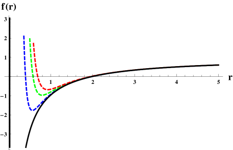
Figure 1: Metric function versus $r$ for $M=q=1$, and $\alpha=0$ (black), -0.2 (blue), -0.4 (green) and -0.6 (red).

The line element for a charged BH with Weyl corrections is given as [29]

$$ds^{2}=f(r)dt^{2}-\frac{1}{f(r)}dr^{2}-R(r)(d\theta^{2}+\sin^{2}\theta d\phi^{2}),$$ (1)

with

$$f(r)=1-\frac{2M}{r}+\frac{q^{2}}{r^{2}}-\frac{4\alpha q^{2}}{3r^{4}}+\frac{40\alpha Mq^{2}}{9r^{5}}-\frac{104\alpha q^{4}}{45r^{6}},\quad R(r)=r^{2}+\frac{4\alpha q^{2}}{9r^{2}},$$ (2)

where $M$, $q$ and $\alpha$ represent the mass, charge and Weyl coupling parameter, respectively. From the graphical analysis of Figure 1, we can see that negatively higher values of the Weyl correction result in the appearance of naked singularities. Moreover, $\alpha=0$ (no Weyl corrections) causes a negative asymptote which shows that the solution has only one horizon. A detailed analysis of the horizons and static limit surface has been discussed in [29]. It is noted that for $\alpha=0$, the above metric reduces to the RN solution. The event horizon $(r_{+})$ of the BH can be determined by setting $f(r_{+})=0$. For the considered line-element, the explicit expression of BH horizon cannot be obtained due to the presence of higher-order terms in the metric potential. Setting $f(r_{+})=0$, the mass of the BH in terms of $r_{+}$ is expressed as

$$M=\frac{45r_{+}^{6}+45q^{2}r_{+}^{4}-60\alpha q^{2}r_{+}^{2}-104\alpha q^{4}}{10r_{+}\left(9r_{+}^{4}-20\alpha q^{2}\right)}.$$ (3)

Hawking proposed that the radiation spectrum emitted from the BH assists to determine its thermodynamic properties [30]. In BH physics, Hawking temperature has analogy with its surface gravity $(\kappa=\frac{f^{{}^{\prime}}(r_{+})}{2})$ as

$$\kappa=\frac{81r_{+}^{8}(q^{2}-r_{+}^{2})+16\alpha^{2}\left(26q^{6}-15q^{4}r_{+}^{2}\right)+\alpha\left(576q^{2}r_{+}^{6}-396q^{4}r_{+}^{4}\right)}{18r_{+}^{7}\left(-9r_{+}^{4}+20\alpha q^{2}\right)}.$$

The corresponding Hawking temperature $(T=\frac{\kappa}{2\pi})$ is calculated as

$$T=\frac{81r_{+}^{8}(q^{2}-r_{+}^{2})+16\alpha^{2}\left(26q^{6}-15q^{4}r_{+}^{2}\right)+\alpha\left(576q^{2}r_{+}^{6}-396q^{4}r_{+}^{4}\right)}{36\pi r_{+}^{7}\left(-9r_{+}^{4}+20\alpha q^{2}\right)},$$ (4)

whose graphical representation with respect to $\alpha$ is displayed in Figure 2. It is observed that the temperature decreases for the larger values of $\alpha$ and $q$. The entropy in terms of area law [17] can be defined as

$$S=\frac{A}{4}=\pi r_{+}^{2}.$$ (5)

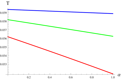
Figure 2: Hawking temperature versus $\alpha$ for $r_{+}=2$ and $q=0.2$ (blue), 0.4 (green) and 0.6 (red).

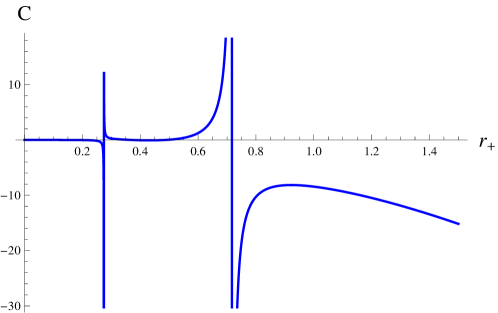
Figure 3: Heat capacity versus $r_{+}$ for $q=0.2$.

In order to investigate thermodynamic stability of BH, we evaluate heat capacity $(C=T\frac{\partial S}{\partial T})$ as follows

$$C = -2\pi r_{+}^{2}\left(-9r_{+}^{4}+20\alpha q^{2}\right)\Big{[}81r_{+}^{8}(q^{2}-r_{+}^{2})+16\alpha^{2}\left(26q^{6}-15q^{4}r_{+}^{2}\right)$$ (6)

$$+ \alpha\left(576q^{2}r_{+}^{6}-396q^{4}r_{+}^{4}\right)\Big{]}\Big{[}320\alpha^{3}\left(182q^{8}-75q^{6}r_{+}^{2}\right)$$

$$+ 144\alpha^{2}q^{4}r_{+}^{4}\left(215r_{+}^{2}-451q^{2}\right)+324\alpha q^{2}r_{+}^{8}\left(72q^{2}-65r_{+}^{2}\right)$$

$$+ 729r_{+}^{12}\left(r_{+}^{2}-3q^{2}\right)\Big{]}^{-1}.$$

It is known that BH is thermodynamical stable for positive values of heat capacity whereas its negative values lead the system towards instability [31]. Figure 3 shows that the heat capacity diverges at two points $(r_{+}=0.27,0.72)$ which leads to the second-order phase transition. The heat capacity remains positive around the first divergence point while it changes from negative to positive at the second point. Thus, small BHs are thermodynamically more stable as compared to the large ones.

Now we investigate the relation between Davies point and QNMs. Since the explicit expression of BH horizon cannot be obtained due to the presence of higher-order terms in the metric potential, we neglect the higher-order terms and take the radial potential as follows

$$f(r)=1-\frac{2M}{r}+\frac{q^{2}}{r^{2}}-\frac{4\alpha q^{2}}{3r^{4}}.$$ (7)

Consequently, the temperature is

$$T=\frac{8\alpha q^{2}+3Mr_{+}^{3}-3q^{2}r_{+}^{2}}{6\pi r_{+}^{5}}.$$ (8)

The corresponding heat capacity can be expressed as

$$C=-\frac{2\pi r_{+}^{2}\left(8\alpha q^{2}+3r_{+}^{2}\left(Mr_{+}-q^{2}\right)\right)}{40\alpha q^{2}+6Mr_{+}^{3}-9q^{2}r_{+}^{2}}.$$ (9)

The divergence point of heat capacity is known as Davies point which measures a phase transition of the BH between thermodynamic stable and unstable phases. In order to determine the divergence point of heat capacity, the following identity must hold

$$40\alpha q^{2}+6Mr_{+}^{3}-9q^{2}r_{+}^{2}=0.$$ (10)

Here, it is difficult to compute the divergence point as $q$ cannot be evaluated in terms of $M$ explicitly. Therefore, we plot the heat capacity to determine its physical behavior as well as divergence point. Figure 4 shows that BH is thermodynamically stable and becomes unstable for $q>0.507$. Also, heat capacity diverges at $q=0.55$ which indicates the first-order phase transition.

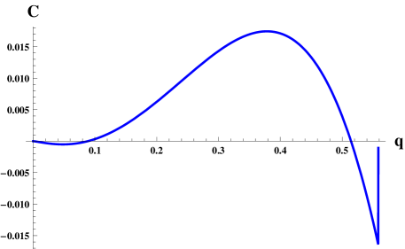
Figure 4: Heat capacity versus $q$ for $\alpha=0.0195$.

2.2 Temperature through Quantum Tunneling

Here we use quantum tunneling approach to obtain temperature for the above mentioned BH. We only consider radial trajectories of particles for which Eq.(1) reduces to

$$ds^{2}=f(r)dt^{2}-\frac{1}{f(r)}dr^{2}.$$ (11)

The Klein-Gordon equation with scalar field having mass $m_{\Phi}$ is

$$\hbar^{2}\nabla\Phi-m^{2}_{\Phi}\Phi=0,$$ (12)

where $\hbar$ is the Dirac constant. The corresponding D’Alembertian operator turns out to be

$$\Box\Phi=-\frac{1}{f(r)}\ddot{\Phi}+f(r)\Phi^{{}^{\prime\prime}}+f^{{}^{\prime}}(r)\Phi^{{}^{\prime}}.$$ (13)

This equation can be solved by applying Wentzel-Kramers-Brillouin approximation which relates $\Phi$ with the action $I$ [32]

$$\Phi(t,r)=\exp\left[\frac{-i}{\hbar}I(t,r)\right].$$ (14)

The corresponding Hamilton-Jacobi equation is

$$\dot{I}^{2}-f^{2}(r)I^{{}^{\prime}2}-m^{2}_{\Phi}f(r)=0,$$ (15)

whose solution in terms of radiation energy $E$ and Hamilton characteristic function $W(r)$ can be expressed as $I=-Et+W(r)$. Here

$$W_{\pm}(r)=\pm\int\frac{dr}{f(r)}\sqrt{E^{2}-f(r)m^{2}_{\Phi}},$$ (16)

which represents spatial part of the action for particles going inside $(W_{-})$ and outside $(W_{+})$ the BH.

We consider only the outward moving particles $W_{+}$ and use the spatial metric as $d\sigma^{2}=\frac{dr^{2}}{f(r)}$. Applying the near horizon approximation $f(r)=f(r_{+})+\acute{f}(r_{+})(r-r_{+})+...$, we have $\sigma=\frac{2\sqrt{r-r_{+}}}{\sqrt{\acute{f}(r_{+})}},$ where $0<\sigma<\infty$. In this scenario, Eq.(16) takes the form

$$W(\sigma)=im_{\Phi}\int\sqrt{1-\frac{4E^{2}}{\sigma^{2}m^{2}_{\Phi}\acute{f}^{2}(r_{+})}}d\sigma,$$ (17)

where $W_{+}=W$. Integration of the above expression yields $W(r)=\frac{2\pi iE}{\acute{f}(r_{+})},$ and hence

$$I=\frac{2\pi i}{\acute{f}(r_{+})}E+\text{(real contribution)}.$$ (18)

The tunneling probability of outgoing and incoming particles across the horizons are defined as [33]

$$\text{Prob [out]}=\exp[-2\text{Im}W_{+}],\quad\text{Prob [in]}=\exp[-2\text{Im}W_{-}].$$ (19)

Here, the imaginary part of the action is same for both the incoming and outgoing solutions so they will cancel out the effect of each other. Thus, the tunneling probability for particles can be expressed as

$$\Gamma\propto\frac{\text{Prob[out]}}{\text{Prob[in]}}=\frac{\exp[-2\text{Im}W_{+}]}{\exp[-2\text{Im}W_{-}]}=\exp(-4\text{Im}W_{+}),$$ (20)

through value of $W(r)$, gives rise to

$$\Gamma=\exp\Big{[}-\frac{4\pi E}{\acute{f}(r_{+})}\Big{]}=\exp[-\frac{E}{T}].$$ (21)

Comparing $\Gamma=\exp(-2\text{Im}I)$ with Boltzmann factor (21), we have

$$T_{t}=\frac{E}{2\text{Im}I}=\frac{\acute{f}(r_{+})}{4\pi}.$$

This is exactly the same as that found through surface gravity. It is pointed out that there exists a correlation between emitted particles and leaked information which resolves the information loss paradox, i.e., $\Gamma=\exp(-2\text{Im}I)=e^{\Delta S}$, where $\Delta S$ is the difference between final and initial values of the BH entropy. We plot the solution (14) with respect to horizon radius to understand the behavior of scalar field. Figure 5 represents that the scalar field behaves as damped periodic oscillator which vanishes at horizon. It is indeed a bound state which vanishes at infinity [34].

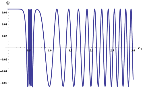
Figure 5: Scalar field versus $r_{+}$ for $m=t=1$ and $E=0.4$, $q$=0.2.

A tachyonic particle is a hypothetical massive particle that always moves faster than the speed of light. It is observed that scalar field is treated as a quantum field and an elementary particle is described as an excitation near the minimum of the scalar potential. The Taylor expansion of the scalar field near the minimum implies that the coefficient of the quadratic term is always positive which means that such a field is not tachyonic. However, if the Taylor expansion near a maximum is observed, then the coefficient of the quadratic term will be negative which leads the system towards tachyonic field [35]. Comparing the derived results with uncharged AdS BH [36], it is found that for $q=0$, all the results reduce to uncharged scenario. The potential behaves as the function of $ae^{-br^{2}}$ which corresponds to the effective potential of tachyon field. It is found that massless scalar field behaves as tachyon field in the absence of dilaton field background. Hence, it depicts the same behavior as found in uncharged AdS BHs.

2.3 Rotating Charged BH with Weyl Corrections

The metric for rotating charged BH with Weyl corrections is defined as [29]

$$ds^{2} = \frac{F(r,\theta)}{\Sigma(r,\theta)}dt^{2}+2\Big{[}1-\frac{F(r,\theta)}{\Sigma(r,\theta)}\Big{]}a\sin^{2}\theta dtd\phi$$ (22)

$$- \Big{[}\frac{\Sigma(r,\theta)\Sigma_{1}(r,\theta)}{F(r,\theta)\Sigma_{1}(r,\theta)+a^{2}\sin^{2}\theta\Sigma(r,\theta)}\Big{]}dr^{2}-\Sigma_{1}(r,\theta)d\theta^{2}$$

$$- \frac{\sin^{2}\theta}{\Sigma(r,\theta)}\Big{[}\Sigma(r,\theta)\Sigma_{1}(r,\theta)+a^{2}\sin^{2}\theta(2\Sigma(r,\theta)-F(r,\theta))\Big{]}d\phi^{2},$$

such that

$$F(r,\theta) = r^{2}+a^{2}\cos^{2}\theta-2Mr+q^{2}$$

$$- \frac{4\alpha q^{2}}{3\left(r^{2}+a^{2}\cos^{2}\theta\right)}\left(1-\frac{50Mr-26q^{2}}{15\left(r^{2}+a^{2}\cos^{2}\theta\right)}\right),$$

$$\Sigma_{1}(r,\theta) = r^{2}+a^{2}\cos^{2}\theta+\frac{4\alpha q^{2}}{9(r^{2}+a^{2}\cos^{2}\theta)},$$

$$\Sigma(r,\theta) = r^{2}+a^{2}\cos^{2}\theta,$$ (23)

where $a$ is the rotation parameter. It is noted that the line-element (4) can be retrieved by setting $a=0$. For simplification, we assume

$$f(r,\theta)=\frac{F(r,\theta)}{\Sigma(r,\theta)}.$$ (24)

Inserting the values of $F(r,\theta)$ and $\Sigma(r,\theta)$ in the above expression leads to

$$f(r,\theta)=1+\frac{q^{2}-2Mr}{a^{2}+r^{2}}-\frac{4\alpha q^{2}\left(15a^{2}+5r(3r-10M)+26q^{2}\right)}{45\left(a^{2}+r^{2}\right)^{3}}.$$ (25)

The corresponding mass can be expressed as

$$M=\frac{45\left(a^{2}+r_{+}^{2}\right)^{2}\left(a^{2}+q^{2}+r_{+}^{2}\right)-4\alpha q^{2}\left(15a^{2}+26q^{2}+15r_{+}^{2}\right)}{90r_{+}\left(a^{2}+r_{+}^{2}\right)^{2}-200\alpha q^{2}r_{+}}.$$ (26)

The Hawking temperature for the rotating charged BH is given by

$$T = \Big{[}-405\left(a^{2}+r_{+}^{2}\right)^{4}\left(a^{2}+q^{2}-r_{+}^{2}\right)-80\alpha^{2}q^{4}\left(15a^{2}+26q^{2}-15r_{+}^{2}\right)$$ (27)

$$+ 36\alpha q^{2}\left(a^{2}+r_{+}^{2}\right)\left(40a^{4}+a^{2}\left(51q^{2}-40r_{+}^{2}\right)+55q^{2}r_{+}^{2}-80r_{+}^{4}\right)\Big{]}$$

$$\times \Big{[}180\pi r_{+}\left(a^{2}+r_{+}^{2}\right)^{3}\left(9\left(a^{2}+r_{+}^{2}\right)^{2}-20\alpha q^{2}\right)\Big{]}^{-1}.$$

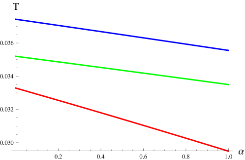
Figure 6: Hawking temperature versus $\alpha$ for $r_{+}=2$, $a=0.2$ and $q$ = 0.2 (blue), 0.4 (green), 0.6 (red).

Figure 6 indicates the decreasing behavior of Hawking temperature with respect to charge and Weyl coupling parameter. In this scenario, the entropy is modified as follows [37]

$$S=\pi(r_{+}^{2}+a^{2}).$$

The corresponding heat capacity takes the form

$$C = \Big{[}2\pi\left(a^{2}+r_{+}^{2}\right)\left(9r_{+}\left(a^{2}+r_{+}^{2}\right)^{2}-20\alpha q^{2}r_{+}\right)^{2}\Big{(}-405\left(a^{2}+r_{+}^{2}\right)^{4}$$ (28)

$$\times \left(a^{2}+q^{2}-r_{+}^{2}\right)-80\alpha^{2}q^{4}\left(15a^{2}+26q^{2}-15r_{+}^{2}\right)+36\alpha q^{2}\left(a^{2}+r_{+}^{2}\right)$$

$$\times \Big{(}40a^{4}+a^{2}\left(51q^{2}-40r_{+}^{2}\right)+55q^{2}r_{+}^{2}-80r_{+}^{4}\Big{)}\Big{)}\Big{]}\Big{[}\Big{(}9\left(a^{2}+r_{+}^{2}\right)^{2}$$

$$- 20\alpha q^{2}\Big{)}\Big{(}3645\left(a^{2}+r_{+}^{2}\right)^{6}\Big{(}a^{4}+a^{2}\left(q^{2}+4r_{+}^{2}\right)+3q^{2}r_{+}^{2}-r_{+}^{4}\Big{)}$$

$$- 1600\alpha^{3}q^{6}\left(15a^{4}+2a^{2}\left(13q^{2}+60r_{+}^{2}\right)+182q^{2}r_{+}^{2}-75r_{+}^{4}\right)$$

$$- 324\alpha q^{2}\left(a^{2}+r_{+}^{2}\right)^{3}\Big{(}65a^{6}+76a^{4}q^{2}+5r_{+}^{4}\left(7a^{2}+72q^{2}\right)+a^{2}r_{+}^{2}$$

$$\times \left(425a^{2}+404q^{2}\right)-325r_{+}^{6}\Big{)}+720\alpha^{2}q^{4}\left(a^{2}+r_{+}^{2}\right)\Big{(}55a^{6}+a^{4}$$

$$\times \left(77q^{2}+435r_{+}^{2}\right)+a^{2}\left(512q^{2}r_{+}^{2}+165r_{+}^{4}\right)+451q^{2}r_{+}^{4}$$

$$- 215r_{+}^{6}\Big{)}\Big{)}\Big{]}^{-1}.$$

Figure 7 shows that $C$ becomes negative for the considered domain and hence the system is unstable for small values of the horizon radius. However, for large values of $r_{+}$, the heat capacity shows positive trend which yields stable BH solution.

Figure 7: Heat capacity versus $r_{+}$ for $\alpha=q=0.2$ and $a=0.8$.

3 Null Geodesic and Quasi-normal Modes

In this section, we discuss null geodesics and photon sphere for the reduced form of the metric function (7). We evaluate Lyapunov exponent and angular velocity using the photon sphere radius. The appropriate form of Lagrangian in the equatorial plane ($\theta=0,\frac{\pi}{2}$) is given as [15]

$$2\mathcal{L}=g_{tt}\dot{t}^{2}-\dot{r}^{2}g_{rr}-g_{\phi\phi}\dot{\phi}^{2}.$$ (29)

The corresponding generalized momentum ($\mathcal{P}_{u}=\frac{\partial\mathcal{L}}{\partial\dot{x}^{u}}=g_{uv}\dot{x}^{v}$) leads to

$$\mathcal{P}_{t}=f(r)\dot{t}\equiv\bar{E},\quad\mathcal{P}_{\phi}=-R\dot{\phi}\equiv-l,\quad\mathcal{P}_{r}=-\frac{\dot{r}}{f(r)},$$ (30)

where $\bar{E}$ and $l$ are the conservation constants which represent the energy and angular momentum of the photon, respectively. Using Eq.(30), $t$ and $\phi$-motions can be computed as

$$\dot{t}=\frac{\bar{E}}{f(r)},\quad\dot{\phi}=\frac{l}{R}.$$

The corresponding Hamiltonian for the null geodesics reads

$$2\mathcal{H}=f(r)\dot{t}^{2}-\frac{\dot{r}^{2}}{f(r)}-R\dot{\phi}^{2}=\bar{E}\dot{t}-l\dot{\phi}-\frac{\dot{r}^{2}}{f(r)}=0,$$ (31)

leading to

$$\dot{r}^{2}+V_{eff}=0,\quad V_{eff}=\frac{l^{2}}{r^{2}}f(r)-\bar{E}^{2},$$ (32)

where $V_{eff}$ denotes the effective potential. It is observed that for $\dot{r}^{2}>0$, the effective potential must be negative which restricts photon to come out at the region of negative potential. Thus, the photon will fall into the BH for small value of angular momentum while for its larger values, the photon will bounce back before it falls into the BH. Between these cases, there exist another phase where photon rounds the BH at radial distance with zero radial velocity [38]. These orbits are known as photon sphere that can be determined through the following conditions

$$V_{eff}=0,\quad\frac{\partial V_{eff}}{\partial r}=0,\quad\frac{\partial^{2}V_{eff}}{\partial r^{2}}<0.$$ (33)

The first condition leads to the photon sphere radius $(r_{ps})$ while the third condition gives the idea about instability of photon sphere and links to QNMs of the BH. Inserting Eq.(32) into the second condition, we have

$$2f(r_{ps})-r_{ps}f^{{}^{\prime}}(r_{ps})=0,$$ (34)

which, in accordance with Eq.(7), gives rise to

$$r_{ps}^{4}-3Mr_{ps}^{3}+2q^{2}r_{ps}^{2}-4\alpha q^{2}=0.$$ (35)

The radius of the photon sphere is given by

$$r_{ps} = \frac{3M}{4}+\frac{1}{2}\sqrt{\frac{27M^{3}-24Mq^{2}}{4\sqrt{\frac{B}{3A}+\frac{A}{3\sqrt[3]{2}}+\frac{9M^{2}}{4}-\frac{4q^{2}}{3}}}-\frac{B}{3A}-\frac{A}{3\sqrt[3]{2}}+\frac{9M^{2}}{2}-\frac{8q^{2}}{3}}$$ (36)

$$+ \frac{1}{2}\sqrt{\frac{B}{3A}+\frac{A}{3\sqrt[3]{2}}+\frac{9M^{2}}{4}-\frac{4q^{2}}{3}},$$

where

$$A = \Big{(}-972\alpha M^{2}q^{2}+\sqrt{\left(-972\alpha M^{2}q^{2}+576\alpha q^{4}+16q^{6}\right)^{2}-4\left(4q^{4}-48\alpha q^{2}\right)^{3}}$$ (37)

$$+ 576\alpha q^{4}+16q^{6}\Big{)}^{\frac{1}{3}},\quad B=4\sqrt[3]{2}\left(q^{4}-12\alpha q^{2}\right).$$

It is noted that for $\alpha=0$, Eq.(37) reduces to RN photon radius [15].

In the eikonal limit $(l\gg 1)$, the QNMs can be defined as [39]

$$w_{Q}=l\Omega-i\Big{(}n+\frac{1}{2}\Big{)}|\lambda|.$$ (38)

Although this correspondence works for a number of cases [40], it may violate whenever the perturbations are gravitational type or the test fields are non-minimally coupled to gravity [41]. Here $n$ represents the number of overtone, $\lambda$ and $\Omega$ are the Lyapunov exponent and angular velocity of the photon sphere given as

$$\Omega=\frac{\dot{\phi}}{\dot{t}}\Big{|}_{r_{ps}}=\frac{f_{ps}}{r_{ps}}=\frac{1}{l_{ps}},\quad\lambda=\sqrt{\frac{-V_{eff}^{{}^{\prime\prime}}}{2\dot{t}^{2}}}\Big{|}_{r_{ps}}=\sqrt{\frac{f_{ps}(2f_{ps}-r_{ps}^{2}f_{ps}^{{}^{\prime\prime}})}{2r_{ps}^{2}}}.$$ (39)

Using Eq.(7), these become

$$\Omega = \frac{\sqrt{\frac{q^{2}+r_{ps}^{2}-2Mr_{ps}}{r_{ps}^{2}}-\frac{4\alpha q^{2}}{3r_{ps}^{4}}}}{r_{ps}},$$

$$\lambda = \sqrt{\frac{\left(12\alpha q^{2}-2q^{2}r_{ps}^{2}+r_{ps}^{4}\right)\left(3r_{ps}^{2}\left(r_{ps}(r_{ps}-2M)+q^{2}\right)-4\alpha q^{2}\right)}{3r_{ps}^{10}}}.$$

To analyze the physical behavior, we plot the above expressions versus charge. It is noted that $\lambda$ shows increasing behavior from $q=0.53$ as the system is not defined for smaller values of charge (left plot of Figure 8). In the right plot, $\Omega$ depicts negative behavior starting from $q=0.51$ and shows decreasing trend for large choices of $q$. It is interesting to mention here that Davies point calculated from Figures 4 and 8 has approximately the same value and lies in the range $(0.51,0.57)$. The deviation between these values is $6\%$.

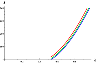
Figure 8: Plots of angular velocity and Lyapunov exponent versus $q$ for $\alpha=0.02$ (blue), 0.0198 (green) and 0.0195 (red).

4 Thermal Fluctuations

This section will analyze the effects of thermal fluctuations on thermodynamic potentials of charged BH with Weyl corrections. The corrected as well as uncorrected thermodynamic expressions for entropy, Helmholtz free energy, internal energy, pressure, enthalpy and specific heat, respectively are computed. Considering Eq.(2) and setting $f(r_{+})=0$, we have

$$45r_{+}^{6}-90Mr^{5}+45q^{2}r_{+}^{4}-60\alpha q^{2}r_{+}^{2}+200\alpha q^{2}Mr_{+}=0.$$ (40)

The Hawking temperature in terms of $M$ is obtained as

$$T=\frac{4\alpha q^{2}\left(5r_{+}(6r_{+}-25M)+78q^{2}\right)+45r_{+}^{4}\left(Mr_{+}-q^{2}\right)}{90\pi r_{+}^{7}}.$$ (41)

To investigate the exact expression of entropy against thermal fluctuations, the partition function is described as [27]

$$Z(\beta)=\int_{0}^{\infty}dE\rho(E)\exp(-\beta E),$$ (42)

Using inverse Laplace transform, the density of states is calculated as

$$\rho(E)=\frac{1}{2\pi i}\int_{\beta_{0}-i\infty}^{\beta_{0}+i\infty}d\beta Z(\beta)\exp(\beta E)=\frac{1}{2\pi i}\int_{\beta_{0}-i\infty}^{\beta_{0}+i\infty}d\beta\exp(\tilde{S}(\beta)).$$ (43)

where $\tilde{S}(\beta)=\ln Z(\beta)+\beta E$ is known as exact entropy for the BH which explicitly depends on temperature. Employing the method of steepest descent, we have

$$\tilde{S}(\beta)=S+\frac{1}{2}(\beta-\beta_{0})^{2}\frac{\partial^{2}\tilde{S}(\beta)}{\partial\beta^{2}}\Big{|}_{\beta=\beta_{0}}+\text{(higher-order terms)},$$ (44)

where $S$ represents equilibrium entropy with $\frac{\partial\tilde{S}}{\partial\beta}=0$ and $\frac{\partial^{2}\tilde{S}}{\partial\beta^{2}}>0$. Inserting the above expression in (43), we have

$$\rho(E)=\frac{\exp(S)}{2\pi i}\int d\beta\exp\Big{(}\frac{1}{2}(\beta-\beta_{0})^{2}\frac{\partial^{2}\tilde{S}(\beta)}{\partial\beta^{2}}\Big{)},$$ (45)

which can further be simplified as [28]

$$\rho(E)=\frac{\exp(S)}{\sqrt{2\pi}}\Big{[}\Big{(}\frac{\partial^{2}\tilde{S}(\beta)}{\partial\beta^{2}}\Big{)}\Big{|}_{\beta=\beta_{0}}\Big{]}^{-\frac{1}{2}}.$$ (46)

Eventually, this leads to

$$\tilde{S}=S-\frac{1}{2}\ln(ST^{2})+\frac{\eta}{S}.$$ (47)

Without loss of generality, we can replace the factor $\frac{1}{2}$ with a more general parameter $\gamma$. In this scenario, the corrected entropy around thermal equilibrium reads [42]

$$\tilde{S}=S-\gamma\ln(ST^{2})+\frac{\eta}{S},$$ (48)

where $\gamma$ and $\eta$ are correction parameters.

• For $\gamma,~{}\eta\rightarrow 0$, the original BH entropy (entropy without any correction terms) can be obtained.

• For $\gamma\rightarrow 1,~{}\eta\rightarrow 0$, the usual logarithmic corrections can be recovered.

• For $\gamma\rightarrow 0,~{}\eta\rightarrow 1$, the second order correction terms can be obtained which is inversely proportional to original BH entropy.

• Finally, for $\gamma,~{}\eta\rightarrow 1$, higher order corrections can be recovered.

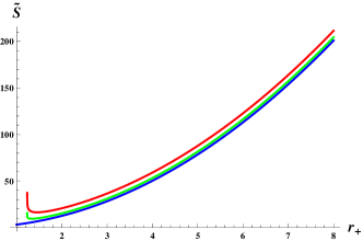
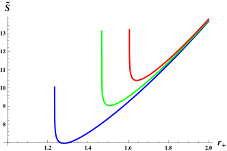
Figure 9: Entropy versus $r_{+}$ for $M=q=1$. We take $\alpha=0.2$ , $\gamma=0$ (blue), 0.5 (green), 1.5 (red) for left plot and $\gamma=0.2$ , $\alpha=0.2$ (blue), 0.6 (green), 1(red) for right plot.

Here, we consider the second case $(\gamma\rightarrow 1,~{}\eta\rightarrow 0)$. We see that the second term in the expression (48) is logarithmic in nature which yields the impact of leading-order corrections to entropy. Inserting Eqs.(5) and (41) in (48), the perturbed form of entropy becomes

$$\tilde{S} = \pi r_{+}^{2}+\gamma\ln\left(8100\pi r_{+}^{12}\right)-2\gamma\ln\Big{(}4\alpha q^{2}\left(5r_{+}(6r_{+}-25M)+78q^{2}\right)$$ (49)

$$+ 45r_{+}^{4}\left(Mr_{+}-q^{2}\right)\Big{)}.$$

Figure 9 represents that the entropy of the system remains positive throughout the considered domain as well as monotonically increasing for the large BH. The entropy decreases upto a certain value of the horizon radius which increases gradually for the larger values of $\gamma$ (left plot) and $\alpha$ (right plot). It is interesting to mention here that thermal fluctuations are effective for small BH while the large BHs are unaffected.

In the presence of thermal fluctuations, the modified first law of BH thermodynamics takes the form [22]

$$\delta M-\mathcal{T}\delta\tilde{S}-\varphi\delta q-\mathcal{V}\delta P=0,$$ (50)

where $\varphi$, $\mathcal{V}$ and $P$ denote the electric potential, volume and pressure, respectively. The potential functions can be obtained through the following relations

$$\mathcal{T}=\Big{(}\frac{\partial M}{\partial\tilde{S}}\Big{)}_{q},\quad\varphi=\Big{(}\frac{\partial M}{\partial q}\Big{)}_{\tilde{S}},\quad\mathcal{V}=\Big{(}\frac{\partial M}{\partial P}\Big{)}_{\tilde{S},q},$$

with

$$\mathcal{T} = \Big{[}4\Big{(}\frac{5\gamma\Big{(}4\alpha q^{2}(25M-12r_{+})+9r_{+}^{3}\Big{(}4q^{2}-5Mr_{+}\Big{)}\Big{)}}{4\alpha q^{2}\Big{(}5r_{+}(6r_{+}-25M)+78q^{2}\Big{)}+45r_{+}^{4}\Big{(}Mr_{+}-q^{2}\Big{)}}+\frac{6\gamma}{r_{+}}+\pi r_{+}\Big{)}$$

$$\times \Big{(}20\alpha q^{2}r_{+}-9r_{+}^{5}\Big{)}^{2}\Big{]}^{-1}\Big{[}\alpha^{2}\Big{(}240q^{4}r_{+}^{2}-416q^{6}\Big{)}+36\alpha\Big{(}11q^{4}r_{+}^{4}-16q^{2}r_{+}^{6}\Big{)}$$

$$+ 81r_{+}^{8}\Big{(}r_{+}^{2}-q^{2}\Big{)}\Big{]},$$

$$\varphi = \Big{[}\gamma q\Big{(}16\alpha^{2}\Big{(}26q^{6}-15q^{4}r_{+}^{2}\Big{)}+\alpha\Big{(}576q^{2}r_{+}^{6}-396q^{4}r_{+}^{4}\Big{)}+81r_{+}^{8}(q-r_{+})$$

$$\times (q+r_{+})\Big{)}\Big{(}4\alpha\Big{(}5r_{+}(6r_{+}-25M)+156q^{2}\Big{)}-45r_{+}^{4}\Big{)}\Big{]}\Big{[}r_{+}\Big{(}20\alpha q^{2}-9r_{+}^{4}\Big{)}^{2}$$

$$\times \Big{(}4\alpha q^{2}\Big{(}\gamma\Big{(}-625Mr_{+}+468q^{2}+120r_{+}^{2}\Big{)}+\pi r_{+}^{2}\Big{(}5r_{+}(6r_{+}-25M)$$

$$+ 78q^{2}\Big{)}\Big{)}+45r_{+}^{4}\Big{(}\gamma\Big{(}Mr_{+}-2q^{2}\Big{)}+\pi r_{+}^{2}\Big{(}Mr_{+}-q^{2}\Big{)}\Big{)}\Big{)}\Big{]}^{-1},$$

$$\mathcal{V} = \frac{4}{3}r_{+}\Big{(}-6\gamma\log\Big{(}4\alpha q^{2}\Big{(}5r_{+}(6r_{+}-25M)+78q^{2}\Big{)}+45r_{+}^{4}\Big{(}Mr_{+}-q^{2}\Big{)}\Big{)}$$

$$+ 3\gamma\log\Big{(}8100\pi r_{+}^{12}\Big{)}-6\gamma+\pi r_{+}^{2}\Big{)}.$$

When we substitute the above values in Eq.(50), it is found that the first law gets satisfied. Thus, it is interesting to mention here that the logarithmic correction terms increase the validity of the first law of thermodynamics. Figure 10 shows the graphical analysis of corrected temperature which indicates that the effect of thermal fluctuations is negligible. Hence, we consider uncorrected temperature along a corrected entropy to observe the effects of logarithmic corrections.

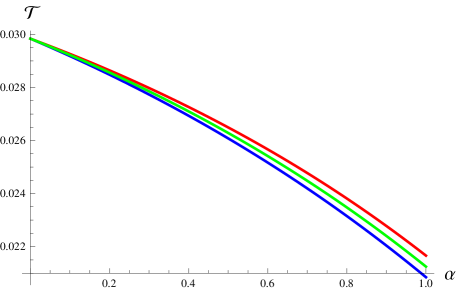
Figure 10: Hawking temperature versus $\alpha$ for $M=q=1$. We take $r_{+}=2$, $\gamma=0$ (blue), 0.5 (green), 1.5 (red).

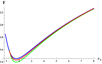
Figure 11: Helmholtz free energy versus $r_{+}$ for $M=q=1$, $\alpha=0.2$ (left plot) and $\gamma=0.2$ (right plot).

Now, we explore thermodynamical equations of state with the help of corrected entropy and Hawking temperature. In this respect, the Helmholtz free energy can be evaluated as

$$F=-\int\tilde{S}dT.$$ (51)

which, through Eqs.(5) and (41), reduces to

$$F = -\frac{1}{9450\pi r_{+}^{7}}\Big{[}2\alpha q^{2}\Big{(}10\gamma\left(7r_{+}(144r_{+}-625M)+2808q^{2}\right)+21\pi r_{+}^{2}$$ (52)

$$\times \left(125r_{+}(4r_{+}-15M)+1092q^{2}\right)\Big{)}+105\gamma\Big{(}4\alpha q^{2}\Big{(}5r_{+}(6r_{+}-25M)$$

$$+ 78q^{2}\Big{)}+45r_{+}^{4}\left(Mr_{+}-q^{2}\right)\Big{)}\Big{(}\ln\left(8100\pi r_{+}^{12}\right)-2\ln\Big{(}4\alpha q^{2}\Big{(}5r_{+}$$

$$\times (6r_{+}-25M)+78q^{2}\Big{)}+45r_{+}^{4}\left(Mr_{+}-q^{2}\right)\Big{)}\Big{)}-1575r_{+}^{4}\Big{(}-3\gamma Mr_{+}$$

$$+ 4\gamma q^{2}+9\pi q^{2}r_{+}^{2}\Big{)}-9450\pi Mr_{+}^{7}\ln(r_{+})\Big{]}.$$

Figure 11 gives the behavior of Helmholtz free energy with respect to $r_{+}$. It is found that the free energy of the small BH increases corresponding to the larger values of Weyl and correction parameters while no effect of fluctuations is observed for the large BH. When the Helmholtz free energy tends to its minimum value, the system shifts towards its equilibrium state and no further work can be extracted from it. Thus, the equilibrium condition of maximum entropy becomes the condition of minimum Helmholtz free energy held at constant temperature. The internal energy for the considered BH solution is given by [27]

$$\mathcal{U}=F+T\tilde{S}.$$ (53)

Substituting the values of $F$, $T$ and $S$ in the above identity, it follows that

$$\mathcal{U} = \frac{1}{9450\pi r_{+}^{7}}\Big{(}-2\alpha q^{2}\Big{(}10\gamma\left(7r_{+}(144r_{+}-625M)+2808q^{2}\right)$$ (54)

$$+ 21\pi r_{+}^{2}\left(25r_{+}(8r_{+}-25M)+312q^{2}\right)\Big{)}+1575r_{+}^{4}$$

$$\times \Big{(}\gamma\left(4q^{2}-3Mr_{+}\right)+3\pi r_{+}^{2}\left(Mr_{+}+2q^{2}\right)\Big{)}$$

$$+ 9450\pi Mr_{+}^{7}\ln(r_{+})\Big{)}.$$

Figure 12 shows that the internal energy becomes negative before the critical value of the horizon radius due to thermal fluctuations whereas for $\gamma=0$, this remains positive throughout the system. However, after the critical radius, it observes the same trend as that of Helmholtz free energy.

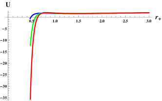
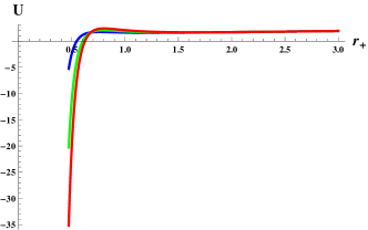
Figure 12: Internal energy versus $r_{+}$ with same values.

The BH volume for considered geometry is defined as [43]

$$V=\frac{4}{3}\pi r_{+}^{3}.$$ (55)

Since spacetime is considered as a thermodynamic system, so we really need to discuss pressure (P). One can calculate BH pressure using the following relation

$$P=-\frac{dF}{dV}=-\frac{dF}{dr_{+}}\frac{dr_{+}}{dV}.$$ (56)

Using Eqs.(52) and (55), the pressure takes the form

$$P = \frac{1}{120\pi^{2}r_{+}^{10}}\Big{[}\left(-8\alpha q^{2}\left(25r_{+}(r_{+}-5M)+91q^{2}\right)-15r_{+}^{4}\left(2Mr_{+}-3q^{2}\right)\right)$$ (57)

$$\times \Big{(}-2\gamma\ln\left(4\alpha q^{2}\left(5r_{+}(6r_{+}-25M)+78q^{2}\right)+45r_{+}^{4}\left(Mr_{+}-q^{2}\right)\right)$$

$$+ \gamma\ln\left(8100\pi r_{+}^{12}\right)+\pi r_{+}^{2}\Big{)}\Big{]}.$$

Figure 13 indicates that the pressure of BH increases significantly for larger values of the considered parameters and coincides with the equilibrium pressure for large values of $r_{+}$. The enthalpy $(H=\mathcal{U}+PV)$ of the system can be obtained as

$$H = \frac{1}{9450\pi r_{+}^{7}}\Big{[}-2\alpha q^{2}\Big{(}10\gamma\left(7r_{+}(144r_{+}-625M)+2808q^{2}\right)+21\pi r_{+}^{2}$$ (58)

$$\times \Big{(}-3125Mr_{+}+2132q^{2}+700r_{+}^{2}\Big{)}\Big{)}-105\gamma\Big{(}8\alpha q^{2}$$

$$\times \left(25r_{+}(r_{+}-5M)+91q^{2}\right)+15r_{+}^{4}\left(2Mr_{+}-3q^{2}\right)\Big{)}\Big{(}\ln\left(8100\pi r_{+}^{12}\right)$$

$$- 2\ln\left(4\alpha q^{2}\left(5r_{+}(6r_{+}-25M)+78q^{2}\right)+45r_{+}^{4}\left(Mr_{+}-q^{2}\right)\right)\Big{)}$$

$$+ 1575r_{+}^{4}\left(\gamma\left(4q^{2}-3Mr_{+}\right)+\pi r_{+}^{2}\left(Mr_{+}+9q^{2}\right)\right)$$

$$+ 9450\pi Mr_{+}^{7}\ln(r_{+})\Big{]}.$$

The effects of fluctuations on the enthalpy is displayed in Figure 14. It is found that enthalpy of the system is an increasing function with respect to horizon radius. Moreover, the corrected as well as equilibrium enthalpy depict the same behavior for different choices of $\alpha$.

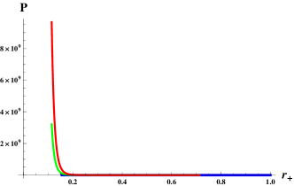
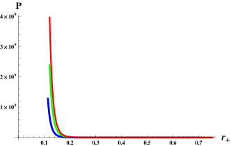
Figure 13: Pressure versus $r_{+}$ with same parameters.

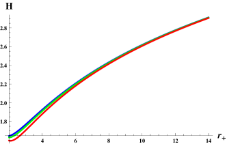
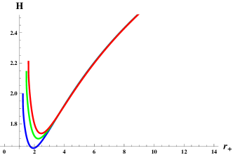
Figure 14: Enthalpy versus $r_{+}$ with same values.

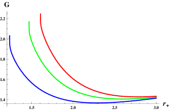
Figure 15: Gibbs free energy versus $r_{+}$ for $M=q=1$, $\alpha=0.2$ (left plot) and $\gamma=0.2$ (right plot).

The corrected Gibbs free energy $(G=H-T\tilde{S})$ is evaluated as [27]

$$G = \frac{1}{9450\pi r_{+}^{7}}\Big{(}-2\alpha q^{2}\Big{(}10\gamma\left(7r_{+}(144r_{+}-625M)+2808q^{2}\right)$$ (59)

$$+ 21\pi r_{+}^{2}\left(125r_{+}(8r_{+}-35M)+2912q^{2}\right)\Big{)}-525\gamma\Big{(}4\alpha q^{2}$$

$$\times \Big{(}-75Mr_{+}+52q^{2}+16r_{+}^{2}\Big{)}+3r_{+}^{4}\left(5Mr_{+}-6q^{2}\right)\Big{)}$$

$$\times \Big{(}\ln\left(8100\pi r_{+}^{12}\right)-2\ln\Big{(}4\alpha q^{2}\left(5r_{+}(6r_{+}-25M)+78q^{2}\right)$$

$$+ 45r_{+}^{4}\left(Mr_{+}-q^{2}\right)\Big{)}\Big{)}+1575r_{+}^{4}\Big{(}\gamma\left(4q^{2}-3Mr_{+}\right)$$

$$- 2\pi r_{+}^{2}\left(Mr_{+}-6q^{2}\right)\Big{)}+9450\pi Mr_{+}^{7}\ln(r_{+})\Big{)}.$$

Figure 15 provides that Gibbs free energy decreases against thermal fluctuations (left plot). The right plot shows the opposite trend, i.e., Gibbs free energy increases for larger values of Weyl parameter. In order to examine the stability of charged BH with Weyl corrections, the specific heat $(C_{S}=\frac{d\mathcal{U}}{dT})$ [27] is calculated as

$$C_{S} = \Big{[}2\Big{(}4\alpha q^{2}\Big{(}\gamma\left(-625Mr_{+}+468q^{2}+120r_{+}^{2}\right)+\pi r_{+}^{2}\Big{(}5r_{+}(6r_{+}-25M)$$ (60)

$$+ 78q^{2}\Big{)}\Big{)}$$

$$+ 45r_{+}^{4}\left(\gamma\left(Mr_{+}-2q^{2}\right)+\pi r_{+}^{2}\left(Mr_{+}-q^{2}\right)\right)\Big{)}\Big{]}\Big{[}3\Big{(}15r_{+}^{4}\left(3q^{2}-2Mr_{+}\right)$$

$$- 8\alpha q^{2}\left(25r_{+}(r_{+}-5M)+91q^{2}\right)\Big{)}\Big{]}^{-1}.$$

Figure 16 represents that specific heat diverges at $r_{+}=0.8$ indicating the phase transition of charged BH. We note that specific heat is negative before the phase transition which shows that small BHs are unstable under the fluctuations while becomes stable after phase transition as heat capacity attains positive values.

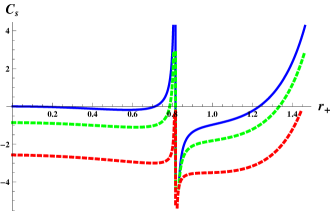
Figure 16: Specific heat versus $r_{+}$ for $M=q=1$, $\alpha=0.2$ (left plot) and $\gamma=0.2$ (right plot).

We can check stability of the system with the help of Hessian matrix which contains second derivatives of Helmholtz free energy with respect to temperature $T$ and chemical potential $\upsilon=\Big{(}\frac{\partial M}{\partial q}\Big{)}_{r_{+}}$. The Hessian matrix is given by [21]

$$H=\left(\begin{array}[]{cc}H_{11}&H_{12}\\ H_{21}&H_{22}\\ \end{array}\right),$$

where

$$H_{11}=\frac{\partial^{2}F}{\partial T^{2}},\quad H_{12}=\frac{\partial^{2}F}{\partial T\partial\upsilon},\quad H_{21}=\frac{\partial^{2}F}{\partial\upsilon\partial T},\quad H_{22}=\frac{\partial^{2}F}{\partial\upsilon^{2}}.$$

The determinant of matrix implies that one of the eigenvalues is zero as $H_{11}H_{22}=H_{12}H_{21}$. Thus, we use trace of the matrix to determine the stability given by

$$\tau\equiv Tr(H)=H_{11}+H_{22}.$$

A necessary criterion for the stable spacetime is the positivity of trace of the Hessian matrix, i.e., $Tr(H)\geq 0$ [44]. From the graphical analysis of trace with respect to horizon (Figure 17), it is clear that small black holes fulfill the stability criterion while the large ones depict unstable behavior. Hence, we find that the Weyl and logarithmic corrections significantly affect the critical point as well as stability of small BHs.

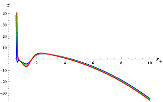
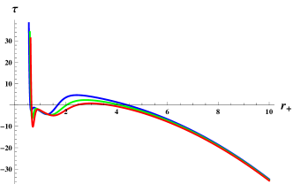
Figure 17: Hessian trace versus $r_{+}$ for $M=q=1$. We take $\alpha=0.2$ , $\gamma=0.5$ (blue), -0.5 (green), 0 (red) for left plot and $\gamma=0.2$, $\alpha=0.5$ (blue), -0.5 (green), 0 (red) for right plot.

5 Concluding Remarks

In this paper, we have studied thermodynamic quantities, QNMs as well as logarithmic corrections for non-rotating charged BH with Weyl corrections. Firstly, the Hawking temperature is computed through surface gravity as well as quantum tunneling and obtained the same result. We have then used null geodesics as well as photon sphere radius to derive relation between Davies point and QNMs. We have also discussed the effect of logarithmic corrections and compared the results of corrected as well as uncorrected thermodynamic potentials through graphical analysis. We have found that heat capacity diverges at $r_{+}=0.27,0.72$ and attained positive values for small charged BH (non-rotating) but BH (rotating) is stable for larger values of horizon radius. It is noted that the Weyl coupling parameter decreases the temperature of BH for both rotating as well as non-rotating scenarios. We have observed that Hawking temperature of non-rotating charged BH is slightly larger than the rotating (Figures 2 and 6).

Secondly, we have investigated the relation between QNMs and Davies point which provides real as well as imaginary parts of QNMs as angular velocity and Lyapunov exponent, respectively. It is shown that the Lyapunov exponent increases for larger values of charge while angular velocity shows opposite behavior for the considered domain. We would like to mention here that Davies points calculated from heat capacity and QNMs have approximately the same values, i.e., $0.57$ and $0.51$, respectively with $6\%$ deviation. This is less than the deviation measured for the charged BH without correction parameter [15].

Finally, we have considered the first-order logarithmic corrections to entropy that modify all given thermodynamic potentials except temperature which is similar to isothermal process. It is seen that entropy is positive valued function and shows decreasing (increasing) behavior for the smaller (larger) values of $r_{+}$. For small horizon radius, the Helmholtz free energy decreases corresponding to larger fluctuation parameter and coincides with the equilibrium state for large values of $r_{+}$ which shows that thermal fluctuations only affect the small BH geometries. The internal energy becomes negative for the smaller values of horizon radius which implies that the temperature of the BH falls due to thermal fluctuations.

The behavior of Gibbs free energy is positive and shows a decreasing trend for larger values of $\gamma$ which indicates that reactions occur inside the BHs are non-spontaneous, i.e., BH requires external energy to sustain its equilibrium position. It is found that specific heat is negative for small BH indicating unstable phase while the system is stable for large values of horizon radius in the presence of thermal fluctuations. Hence, thermal fluctuations induce more instability for small and medium BHs while the large BHs remain unaffected. It is worth mentioning here that for $\alpha=0$, all the derived results reduce to RN BH [31, 45].

References

- [1] Easther, R. and Lowe, D.: Phys. Rev. Lett. 82(1999)4967.
- [2] Hawking, S.W.: Commun. Math. Phys. 43(1975)199.
- [3] Page, D.N.: Phys. Rev. D 13(1976)198.
- [4] Steinhauer, J.: Nature Phys. 12(2016)959.
- [5] Michel, F. et al.: Phys. Rev. D 94(2016)084027.
- [6] Vishveshwara, C.V.: Nature 227(1970)936.
- [7] Jing, J. and Pan, Q.: Phys. Lett. B 660(2008)13.
- [8] He, X. et al.: Phys. Lett. B 665(2008)392.
- [9] Konoplya, R.A. and Zhidenko, A.: Rev. Mod. Phys 83(2011)793.
- [10] Konoplya, R.A. and Stuchlik, Z.: Phys. Lett. B 771(2017)597.
- [11] Breton, N. et al.: Int. J. Mod. Phys D 26(2017)1750112.
- [12] Churilova, M.S.: Eur. Phys. J. C 79(2019)629.
- [13] Momennia, M. and Hendi, S.H.: Phys. Rev. D 99(2019)124025.
- [14] Ghaderi, K. and Malakolkalami, B.: Gravit. Cosmol. 24(2018)61.
- [15] Wei, S.W. and Liu, Y.X.: arXiv:1909.11911.
- [16] Wei, S.W. et al.: Phys. Rev. D 99(2019)044013.
- [17] Das, S. et al.: Class. Quantum Grav. 19(2002)2355.
- [18] Sadeghi, J. et al.: Can. J. Phys. 92(2014)1638.
- [19] Faizal, M. and Khalil, M.M.: Int. J. Mod. Phys. A 30(2015)1550144.
- [20] Pourhassan, B. and Faizal, M.: Nucl. Phys. B 913(2016)834.
- [21] Pourhassan, B. et al.: Eur. Phys. J. C 77(2017)555.
- [22] Jawad, A. and Shahzad, M.U.: Eur. Phys. J. C 77(2017)349.
- [23] Zhang, M.: Nucl. Phys. B 935(2018)170.
- [24] Sinha, A.K. et al.: arxiv:1608.08359.
- [25] Upadhyay, S. et al.: Prog. Theor. Exp. Phys. 2018(2018)093E01.
- [26] Haldar, A. and Biswas, R.: Gen. Relativ. Gravit. 51(2019)35.
- [27] Pourhassan, B. and Upadhyay, S.: arXiv:1910.11698.
- [28] Pradhan, P.: Universe 5(2019)57.
- [29] Chen, S. and Jing, J.: Phys. Rev. D 89(2014)104014.
- [30] Ding, C.: Int. J. Theor. Phys. 53(2014)694.
- [31] Altamirano, N. et al.: Galaxies 2(2014)89.
- [32] Kim, H.: Phys. Lett. B 703(2011)94.
- [33] Sharif, M. and Javed, W.: Eur. Phys. J. C 72(2012)1997.
- [34] Pourhassan, B.: Mod. Phys. Lett. A 31(2016)1650057.
- [35] Myung, Y.S. and Zou, D.C.: Eur. Phys. J. C 79(2019)273.
- [36] Sadeghi, J. et al.: Int. J. Theor. Phys. 50(2011)129.
- [37] Ruiz, O. et al.: J. Phys. Conf. 1219(2019)012016
- [38] Wei, S.W. and Liu, Y.X.: Phys. Rev. D 97(2018)104027.
- [39] Cardoso, V. et al.: Phys. Rev. D 79(2009)064016.
- [40] Breton, N. et al.: Int. J. Mod. Phys. B 26(2017)1750112.
- [41] Konoplya, R.A. et al.: Phys. Rev. D 98(2018)104033.
- [42] Pourhassan, B., Kokabi, K. and Sabery, Z.: Ann. Phys. 399(2018)181; Pourhassan, B. and Kokabi, K.: Int. J. Theor. Phys 57(2018)780; Pourhassan, B. et al.: Gen. Relativ. Gravit. 49(2017)144.
- [43] Pourhassan, M. and Faizal, M.: Europhys. Lett. 111(2015)40006.
- [44] Cuadros-Melgar, B. et al.: arxiv:2003.00564.
- [45] Moinuddin, A.S.M. and Ali, M.H.: Int. J. Mod. Phys. A 34(2019)1950211.