Redshift evolution of the underlying type Ia supernova stretch distribution

The detailed nature of type Ia supernovae (SNe Ia) remains uncertain, and as survey statistics increase, the question of astrophysical systematic uncertainties arises, notably that of the evolution of SN Ia populations. We study the dependence on redshift of the SN Ia SALT2.4 light-curve stretch, which is a purely intrinsic SN property, to probe its potential redshift drift. The SN stretch has been shown to be strongly correlated with the SN environment, notably with stellar age tracers. We modeled the underlying stretch distribution as a function of redshift, using the evolution of the fraction of young and old SNe Ia as predicted using the SNfactory dataset, and assuming a constant underlying stretch distribution for each age population consisting of Gaussian mixtures. We tested our prediction against published samples that were cut to have marginal magnitude selection effects, so that any observed change is indeed astrophysical and not observational in origin. In this first study, there are indications that the underlying SN Ia stretch distribution evolves as a function of redshift, and that the age drifting model is a better description of the data than any time-constant model, including the sample-based asymmetric distributions that are often used to correct Malmquist bias at a significance higher than 5 $\sigma$. The favored underlying stretch model is a bimodal one, composed of a high-stretch mode shared by both young and old environments, and a low-stretch mode that is exclusive to old environments. The precise effect of the redshift evolution of the intrinsic properties of a SN Ia population on cosmology remains to be studied. The astrophysical drift of the SN stretch distribution does affect current Malmquist bias corrections, however, and thereby the distances that are derived based on SN that are affected by observational selection effects. We highlight that this bias will increase with surveys covering increasingly larger redshift ranges, which is particularly important for the Large Synoptic Survey Telescope.

1 Introduction

Type Ia supernovae (SNe Ia) are powerful cosmological distance indicators that enabled the discovery that the Universe’s expansion accelerates (Riess et al., 1998; Perlmutter et al., 1999). They remain a key cosmological probe today for understanding the properties of dark energy (DE) because they are the only tool that can precisely map the recent expansion rate ($z<0.5$) when DE is driving it (e.g., Scolnic et al., 2019). Type Ia supernovae are also the key to directly measuring the Hubble constant ($H_{0}$) if their absolute magnitude can be calibrated (Riess et al., 2016; Freedman et al., 2019). Interestingly, the value of $H_{0}$ that is derived when the SNe Ia are anchored to Cepheids (the Supernovae, $H_{0}$, for the Equation of State of dark energy project, Riess et al., 2009, 2016) is $\sim 5\sigma$ higher than what is predicted from cosmic microwave background (CMB) data measured by Planck assuming the standard $\Lambda$CDM (Planck Collaboration et al., 2020; Riess et al., 2019; Reid et al., 2019), or when the SN luminosity is anchored at intermediate redshift by the baryon acoustic oscillation (BAO) scale (Feeney et al., 2019). While using the tip of the red giant branch technique in place of the Cepheids seems to favor an intermediate value of $H_{0}$ (Freedman et al., 2019, 2020), time-delay measurements from strong lensing also appear to favor high $H_{0}$ values (Wong et al., 2020).

The $H_{0}$ conundrum has received much attention because it could be a sign of new fundamental physics. No simple solution is so far able to accommodate this $H_{0}$ conundrum when all other probes are accounted for, however (Knox & Millea, 2020). Alternatively, systematic effects affecting one or several of the aforementioned analyses might explain at least some of this discrepancy. Rigault et al. (2015) suggested that SNe Ia from the Cepheid calibrator sample differ by construction from those in the Hubble flow sample, as the former strongly favors young stellar populations while the latter does not. This selection effect would affect the derivation of $H_{0}$ if SNe Ia from young and older environments differed in average standardized magnitudes.

The relation between SNe Ia and their host galaxy properties has been studied extensively. The first key finding was that the standardized SNe Ia magnitudes significantly depend on the host galaxy stellar mass, with SNe Ia from high-mass host galaxies being brighter on average (e.g., Kelly et al., 2010; Sullivan et al., 2010; Childress et al., 2013; Betoule et al., 2014; Kim et al., 2019; Smith et al., 2020). This mass-step correction is currently used in cosmological analyses (e.g., Betoule et al., 2014; Scolnic et al., 2018), including to derive $H_{0}$ (Riess et al., 2016, 2019). The underlying connection between the SNe and their host galaxies remains unclear, however, particularly when global properties such as the host stellar mass are used. This in turn raises the question of the accuracy of such corrections because the global properties of the host galaxies evolve with redshift. More recently, studies have used the local SN host galaxy environment to probe more direct connections between the SNe and their host galaxy environments (Rigault et al., 2013), showing that local age tracers such as the local specific star formation rate (LsSFR) or the local color are more strongly correlated with the standardized SN magnitude (Roman et al., 2018; Kim et al., 2018; Rigault et al., 2020). The identification of SN Ia spectral features that are correlated with LsSFR (Nordin et al., 2018) further support this connection. These results suggest age as the driving parameter underlying the mass step. If this is true, it would have a significant effect for cosmology because the environmental correction that would need to be applied to SN standardization could strongly vary with redshift (Rigault et al., 2013; Childress et al., 2014; Scolnic et al., 2018). The importance of local SN environmental studies remains highly debated, however (e.g., Jones et al., 2015, 2019), and especially the effect of such an astrophysical bias has on the derivation of $H_{0}$ (Jones et al., 2015; Riess et al., 2016, 2018; Rose et al., 2019).

The concept of the SN Ia age dichotomy arose with the study of the SN Ia rate. Mannucci et al. (2005), Scannapieco & Bildsten (2005), Sullivan et al. (2006) and Smith et al. (2012) have shown that the relative SNe Ia rate in galaxies could be explained if two populations existed, a young population that follows the host star formation activity, and an old population that followed the host stellar mass (the so-called prompt-and-delayed or A+B model). Rigault et al. (2020) used the LsSFR to determine the younger (those with a high LsSFR) and the older (those with a low LsSFR) populations. Furthermore, since the first SNe Ia host analyses, the SN stretch has been known to be strongly correlated with the SN host galaxy properties (Hamuy et al., 1996, 2000). This correlation has been extensively confirmed since then (e.g., Neill et al., 2009; Lampeitl et al., 2010; Gupta et al., 2011; D’Andrea et al., 2011; Pan et al., 2014). Following the A+B model and the connection between SN stretch and host galaxy properties, Howell et al. (2007) first discussed the potential redshift drift of the SN stretch distribution. In this paper we revisit this question using the most recent SNe Ia datasets.

We here step aside from the cosmological analyses to probe the validity of our modeling of the SN population, which we claim is constituted of two age populations (Rigault et al., 2013, 2015, 2020): an older and a younger population, the former having lower light-curve stretches on average and being brighter after standardization. We use the correlation between the SN age as probed by the LsSFR and the SN stretch to model the expected evolution of the underlying SN stretch distribution as a function of redshift. This modeling relies on three assumptions: (1) There are two distinct populations of SNe Ia, (2) the relative fraction of each of these populations as a function of redshift follows the model presented in Rigault et al. (2020), and (3) the underlying distribution of stretch for each age sample is constant. This paper tests this specific model with datasets from the literature.

We present the sample we used for this analysis in Section 2. It was derived from the Pantheon catalog (Scolnic et al., 2018). We discuss the importance of obtaining a “complete” sample, that is, a sample that is representative of the true underlying SNe Ia distribution, and how we built one from the Pantheon sample. We then present our modeling of the distribution of stretch in Section 3 and our results in Section 4. In this section, we test whether the SN stretch distribution evolves as a function of redshift and determine whether the aforementioned age model agrees well with this evolution. We briefly discuss these results in the context of SN cosmology in Section 5, and we conclude in Section 6.

2 Complete sample construction

The ideal SN Ia sample for studying this question would be a very deep, large-area, volume-limited sample. This would capture the true underlying stretch distribution function, and we would then study how it evolves with redshift. No such sample exists, therefore we must first construct subsamples from existing high-redshift SN Ia samples that are as near to volume-limited as possible.

2.1 Applying redshift cuts

We based our analysis on the most recent comprehensive SNe Ia compilation, the Pantheon catalog from Scolnic et al. (2018). A naive approach to testing the SN stretch redshift drift would be to simply compare the observed SN stretch distributions in a few redshift bins. In practice, however, differential observational selection effects will affect the observed SN stretch distributions. Because the observed SN Ia magnitude correlates with the light-curve stretch (and color), the first SNe Ia that a magnitude-limited survey will miss are those at the lowest stretch (which are the reddest). Consequently, if magnitude-related observational selection effects are not accounted for, true population drift might be confused with survey properties, and vice versa.

Assuming sufficient (and unbiased) spectroscopic follow-up for acquiring SN types and host galaxy redshifts, the observation selection effects of magnitude-limited surveys should be negligible below a given redshift at which even the faintest normal SNe Ia can be observed. Aiding in the construction of nearly volume-limited subsamples is the fact that the SN Ia population trails off toward fainter SNe Ia. A complication is that complete spectroscopic follow-up has not always been the norm, as discussed below. In contrast, targeted surveys have highly complex observational selection functions and so are discarded from our analysis. High-redshift SN cosmology samples, such as the Pantheon sample, are predominately assembled from magnitude-limited surveys from which volume-limited SN Ia subsamples can be constructed.

We present in Fig. 1 the light-curve stretch and color of SNe Ia from the following surveys: PanStarrs (PS1 Rest et al., 2014), the Sloan Digital Sky Survey (SDSS Frieman et al., 2008), and the SuperNovae Legacy Survey (SNLS Astier et al., 2006). An ellipse in the SALT2.4 $(x_{1},c)$ plane with $x_{1}=\pm 3$ and $c=\pm 0.3$ encapsulates the full parent distribution (Guy et al., 2007; Betoule et al., 2014); see also Bazin et al. (2011) and Campbell et al. (2013) for similar contours, the second using a more conservative $|c|\leq 0.2$ cut. Assuming the SN absolute magnitude with $x_{1}=0$ and $c=0$ is $M_{0}=-19.36$ (Kessler et al., 2009; Scolnic et al., 2014), we can derive the absolute standardized magnitude at maximum of light $M=M_{0}-\alpha x_{1}+\beta c$ within the aforementioned ellipse given the standardization coefficient $\alpha=0.156$ and $\beta=3.14$ from Scolnic et al. (2018): The faintest SN Ia is that with $(x_{1}=-1.65,c=0.25)$ and an absolute standardized magnitude at peak in Bessel $B$ band of $M^{t_{0}}_{\min}=-18.31$ mag. This object typically ought to be detected 5 days before and a week after peak to build a suitable light-curve, the effective limiting standardized absolute magnitude is approximately $M_{\lim}=-18.00$ mag. Hence, given the magnitude limit $m_{\lim}$ of a magnitude limited survey, we can derive the maximum redshift $z_{\lim}$ above which the faintest SNe Ia will be missed using the relation between apparent magnitude, redshift, and absolute magnitude $\mu(z_{\lim})=m_{\lim}-M_{\lim}$.

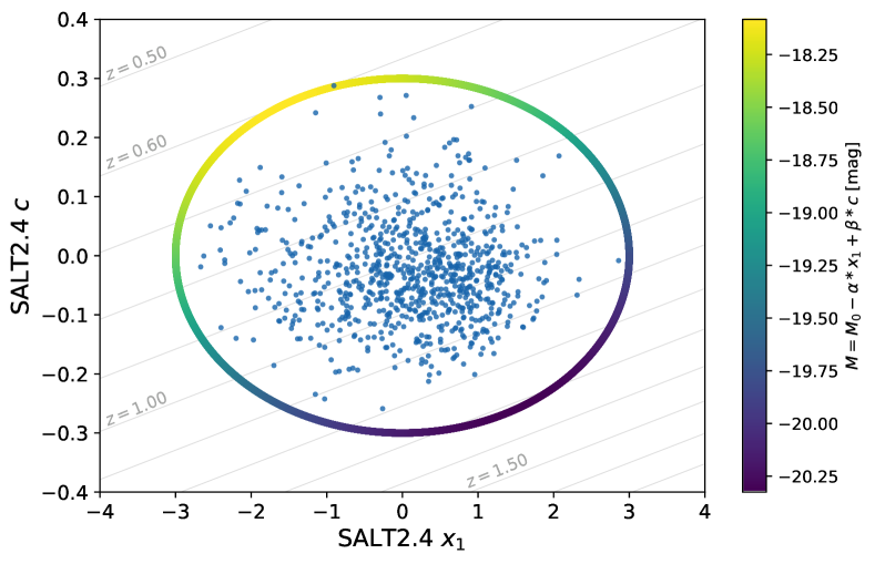
Figure 1: SALT2.4 stretch ($x_{1}$) and color ($c$) light-curve parameters of SNe Ia from the SDSS, PS1, and SNLS samples of the Pantheon catalog. The individual SNe are shown as blue dots. The ellipse $(x_{1}=\pm 3,c=\pm 0.3)$ is displayed, colored by the corresponding standardized absolute magnitude using the $\alpha$ and $\beta$ coefficients from Scolnic et al. (2018). The diagonal gray lines represent the $(x_{1},c)$ evolution for $m=m_{\lim}$ for $z$ between $0.50$ and $z=1.70$ using the SNLS $m_{\lim}$ of $24.8$ mag.

We therefore considered a set of cuts that defines a first fiducial sample, taking the limits as initially suggested by the previous completeness analysis. However, as this solution might be an overly simplified way to create a complete sample, for example, because it ignores spectroscopic follow-up in efficiency for redshifts below $z_{lim}$, we also considered another set of cuts to define a so-called conservative sample. This is smaller and therefore less statistically constraining, but also even less prone to observational selection effects. If the redshift drift is still significant in the conservative sample, it would be even more meaningful in a carefully tailored selection-free sample. These samples are adequate for the goal of this study, which is to develop a first implementation of a model for drift in SN Ia properties. If fruitful, the sample selection can later be refined as required with a more detailed model of the observational selection, for instance, using the SNANA package (Kessler et al., 2009).

The SNLS typically acquired SNe Ia in the redshift range $0.4<z<0.8$; at these redshifts, the rest-frame Bessel $B$ band roughly corresponds to the SNLS $i$ filter, which has a $5\sigma$ depth of 24.8 mag. This converts into a $z_{\lim}=0.60$, in agreement with Neill et al. (2006), Perrett et al. (2010), and Bazin et al. (2011). Fig. 14 of Perrett et al. (2010, see their Section 5), however, suggests a lower limit of $z_{\lim}=0.55$. We therefore used $z=0.60$ and $z=0.55$ as redshift limits for the fiducial and conservative samples, respectively, for the SNLS.

Similarly, PS1 observed SNe Ia in the range $0.2<z<0.4$, their $g$-band $5\sigma$ depth is 23.1 mag (Rest et al., 2014), which yields $z_{\lim}=0.31$, in agreement with Fig. 6 of Scolnic et al. (2018), for example. If we were to be conservative, this figure would also suggest of a more stringent $z_{\lim}=0.27$ cut; we therefore used $0.31$ and $0.27$ for our fiducial and conservative samples, respectively, for PS1.

In a similar redshift range, the SDSS has a limiting magnitude of 22.5 (Dilday et al., 2008; Sako et al., 2008), which would lead to $z_{\lim}=0.24$. However, the SDSS surveys had to contend with limited spectroscopic resources. As discussed in Kessler et al. (2009, Section 2), during the first year of SDSS, SNe Ia with $r<20.5$ mag were favored for spectroscopic follow-up, corresponding to a redshift cut at $0.15$. For the remaining SDSS survey, additional spectroscopic resources were available, and Kessler et al. (2009) and Dilday et al. (2008) showed a reasonable completeness up to $z_{\lim}=0.2$. Based on this, we used $z_{\lim}=0.20$ and $z_{\lim}=0.15$ for our fiducial and conservative samples, respectively, for the SDSS.

The sample selection is summarized in Table 1, and the redshift distribution of these three surveys is shown in Fig. 2. As expected, the selected redshift limits are roughly located slightly before the peak of these histograms. In Section 2.2 we confirm that these redshift limits are effective for constructing nearly volume-limited subsamples from samples that were initially more closely magnitude limited in their search or spectroscopic follow-up.

Table 1: Composition of the SNe Ia dataset used in this analysis. Conservative cuts are indicated in parentheses. The SNf limit is set by Rigault et al. (2020), see text.

Survey	$z_{\lim}$	$N_{\mathrm{SN}}$
SNf	0.08	114
SDSS	0.20 (0.15)	167 (82)
PS1	0.31 (0.27)	160 (122)
SNLS	0.60 (0.55)	102 (78)
HST	–	26
Total	–	569 (422)

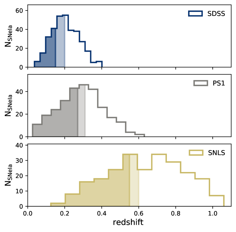
Figure 2: From top to bottom: Redshift histograms of SNe Ia from the SDSS, PS1, and SNLS dataset (data from Pantheon, Scolnic et al. 2018). The colored parts represent the distribution of SNe Ia that we retained in our analysis because they are assumed to be free from observational selection bias (see Section 2). The darker (lighter) color responds to the conservative (fiducial) selection cut.

In addition, we used the SNe Ia from the Nearby Supernova Factory (SNfactory, Aldering et al., 2002) published in Rigault et al. (2020) and that have been discovered from nontargeted searches (114 SNe Ia, see their sections 3 and 4.2.2 ; see Aldering et al. 2020). For this dataset, spectroscopic screening was performed for candidates with $r\lesssim 19.5$; redshift cuts were then applied when selecting which SN Ia to follow, resulting in a redshift range of $0.02<z<0.09$, further reduced to $<0.08$ in Rigault et al. (2020) to extract local host properties. These 114 SNfactory SNe Ia are thus in the volume-limited part of the survey (Aldering et al., in prep.), and are therefore assumed to be a random sampling of the underlying SN population. The SNfactory sample is particularly useful for studying SN property drift because it enables us to have a large complete SN Ia sample at $z<0.1$. Finally, we include the HST sample from Pantheon (Strolger et al., 2004). These high-redshift SNe are of great interest as they provide the greatest leverage for testing evolution. While at these redshifts the supernovae typing is challenging, the target classification was robust enough to include them in the cosmological analysis (Scolnic et al., 2018), and we did not impose further cuts. Section 4 highlights that while compatible with it, our results are not dependent on the inclusion of this dataset.

We present the stretch distribution and redshift histogram of these five surveys up to their respective $z_{\lim}$ in Fig. 3. We observe here that the fraction of low-stretch SNe (typically $x_{1}<-1$) appears to decrease as a function of redshift; this is confirmed in Fig. 6, in which the evolution of the mean stretch is shown, with the data split in redshift bins of regular sample size. SNe Ia at higher redshift have a larger stretch ($0.34\pm 0.10$ at $z\sim 0.65$) on average than those at lower redshift ($-0.17\pm 0.10$ at $z\sim 0.05$), suggesting that the underlying stretch distribution evolves with redshift.

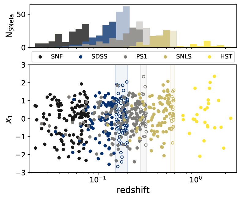
Figure 3: Bottom: SALT2.4 light-curve stretch as a function of redshift for each survey considered in this analysis (see legend). Solid (open) markers correspond to the conservative (fiducial) redshift cuts. Top: Stacked redshift histograms in dark (light) colors for the conservative (fiducial) redshift cuts.

2.2 Testing the construction of a volume-limited sample

In section 2.1 we have built volume-limited samples from a set of magnitude-limited ones using simple redshift cuts. This simplified approach is statistically suboptimal, but should suffice to test our key question whether redshift evolution of stretch is compatible with the model of Rigault et al. (2020). However, the possibility remains that a complex observational selection function related to spectroscopic follow-up efficiencies below our fiducial (or even conservative) redshift cuts might still affect our sample, making it not fully volume limited; this would in turn bias our conclusion about the astrophysical drift of the SNe Ia population. We now examine this possibility.

To test for the existence of potential leftover observational selection biases in our sample, we compared the stretch and color distributions of the SNe Ia originating from different datasets having overlapping redshift ranges: these distributions should be similar if they reflect the underlying parent population. We note that the redshift range has to be narrow enough so that any drift would be negligible.

The two samples that overlap most in redshift are PS1 and SDSS in the redshift range $0.10<z<0.20$ (see Fig 3). This overlapping subsample consists of the 146 SNe Ia at the high-redshift end of SDSS and thus is most likely to be affected by residual observational selection effects (see the corresponding discussion in section 2.1). Over that same redshift range, PS1 has 52 SNe Ia that are in the lowest redshift bins and thus unlikely to have any observational selection issue. To identify potential inconsistency between the PS1 and SDSS subsamples, Fig. 4 (upper panels) compares the stretch and color distribution of these two surveys. The resulting Kolmogorov-Smirnov (KS) similarity test $p$-values ($p>10\%$) do not support any inconsistency, in agreement with the visual impression from Fig. 4.

We performed a similar analysis for PS1 and SNLS over the redshift range $0.20<z<0.31$ (Fig. 4, lower panels), where the same conclusion can be drawn: There is no substantial sign of discrepancy in the stretch and color distributions between the low and high end of our fiducial SNLS and PS1 samples, respectively. Nonetheless, the small size of the SNLS dataset at $z<0.31$ (12 SNe Ia vs. 90 for PS1) limits the sensitivity of this test, and only a strong deviation would be noticeable. Extending the redshift range to $0.20<z<0.40$ (although we have no PS1 data above 0.3) allows increasing the SNLS subsample to 31, but the stretch $p$-value remains high (34%), showing no sign of inconsistency.

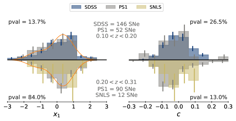
Figure 4: $x_{1}$ (left) and $c$ (right) distribution histograms of different surveys overlapping in redshift. Facing up: SDSS and PS1 within the redshift range $0.10<z<0.20$. Facing down: PS1 and SNLS within the redshift range $0.20<z<0.31$. Error bars show the Poisson noise. Our stretch base model is illustrated in orange at the mean redshift of the redshift ranges, $0.15$ and $0.25$, respectively. Kolmogorov-Smirnov test $p$-values are indicated at the top (bottom) of each panel and show no sign that the SDSS and PS1 (PS1 and SNLS) $x_{1}$ and $c$ distributions are not drawn from the same underlying distributions.

We finally highlight that the SNe Ia color is more prone to observational selection effects than stretch, as illustrated in Fig. 1; see also Fig. 3 of Kessler & Scolnic (2017), for instance. Hence, because the comparison of color distributions shows no significant indication of leftover observational selection effect, this further supports our claim that our simple redshift-based selection criteria are sufficient to build the complete SNe Ia samples required to test the redshift evolution of the stretch distribution.

3 Modeling the redshift drift

Rigault et al. (2020) presented a model for the evolution of the fraction of younger and older SNe Ia as a function of redshift following previous work on rates and delay-time distributions (e.g., Mannucci et al., 2005; Scannapieco & Bildsten, 2005; Sullivan et al., 2006; Smith et al., 2012; Childress et al., 2014; Maoz et al., 2014). In short, it was assumed that the number of young SNe Ia follows the star formation rate (SFR) in the Universe, while the number of old SNe Ia follows the number of billion-old stars in the Universe, that is, the stellar mass (M^∗). Hence, if we denote $\delta(z)$ ($\psi(z)=1-\delta(z)$) the fraction of young (old) SNe Ia in the Universe as a function of redshift, then the ratio $\delta/\psi$ is expected to follow the evolution of the specific star formation rate (SFR/M^∗), which goes as $(1+z)^{2.8}$ until $z\sim 2$ (e.g., Tasca et al., 2015). Since $\delta(0.05)\sim\psi(0.05)$ (Rigault et al., 2013, 2020; Wiseman et al., 2020), in agreement with rate expectations (Mannucci et al., 2006; Rodney et al., 2014), Rigault et al. (2020) concluded that

$$\delta(z)=\left(K^{-1}\times(1+z)^{-2.8}+1\right)^{-1}$$ (1)

with $K=0.87$. This model is comparable to the evolution subsequently predicted by Childress et al. (2014) based on SN rates in galaxies depending on their quenching time as a function of their stellar mass.

3.1 Base underlying stretch distribution

To model the evolution of the full SN stretch distribution as a function of redshift, we need to model the SN stretch distribution for each age subsample given our aforementioned model of the evolution of the fraction of younger and older SNe Ia with cosmic time. Rigault et al. (2020) presented the relation between SN stretch and LsSFR measurement, a progenitor age tracer, using the SNfactory sample. This relation is shown in Fig. 5 for the SNfactory SNe used in the current analysis. Given the structure of the stretch-LsSFR scatter plot, our model of the underlying SN Ia stretch distribution is defined as follows: the stretch distribution of the younger population ($\log(\mathrm{LsSFR})\geq-10.82$) is modeled as a single normal distribution $\mathcal{N}(\mu_{1},\sigma_{1}{}^{2})$, and the stretch distribution of the older population ($\log(\mathrm{LsSFR})<-10.82$) is modeled as a bimodal Gaussian mixture $a\times\mathcal{N}(\mu_{1},\sigma_{1}{}^{2})+(1-a)\times\mathcal{N}(\mu_{2},\sigma_{2}{}^{2})$, where one mode is the same as for the young population, $a$ representing the relative effect of the two modes.

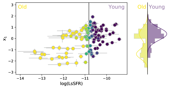
Figure 5: Main: SALT2.4 light-curve stretch ($x_{1}$) as a function of the LsSFR for SNfactory SNe. The color corresponds to the probability, $p_{y}$, for the SNe Ia to be young, i.e., to have $\log\mathrm{LsSFR}\geq-10.82$ (see Rigault et al., 2020). Right: $p_{y}$-weighted histogram of the SN stretches, as well as the adjusted base model; contributions of the younger and older population are shown in purple and yellow, respectively.

The stretch probability distribution function (pdf) of a given SN will be the linear combination of the stretch distributions of these two population weighted by its probability $y^{i}$ to be young (see Section 3.2). In general, however, the fraction of young SNe Ia as a function of redshift is given by $\delta(z)$ (see Eq. 1), and therefore our redshift drift model of the underlying stretch distribution of SNe Ia as a function of redshift $X_{1}(z)$ is given by

$$X_{1}(z)=\delta(z) \times\mathcal{N}(\mu_{1},\sigma_{1}{}^{2})+$$

$$(1-\delta(z)) \times\left[a\times\mathcal{N}(\mu_{1},\sigma_{1}{}^{2})+(1-a)\times\mathcal{N}(\mu_{2},\sigma_{2}{}^{2})\right]$$ (2)

This is our base drifting model.

3.2 Comparison to data

Given the probability $y^{i}$ that a given SN is young and assuming our base model (see Section 3.1), the probability of measuring a SALT2.4 stretch $x_{1}^{i}$ with an error $\mathrm{d}x_{1}^{i}$ is given by

$$\mathcal{P}\left(x^{i}_{1}\mid\@vec{\theta};\mathrm{d}x^{i}_{1},y^{i}\right)=y^{i} \times\mathcal{N}\left(x^{i}_{1}\mid\mu_{1},\sigma_{1}{}^{2}+\mathrm{d}x^{i}_{1}{}^{2}\right)+$$

$$(1-y^{i}) \times\bigg{[}a\times\mathcal{N}\left(x^{i}_{1}\mid\mu_{1},\sigma_{1}{}^{2}+\mathrm{d}x^{i}_{1}{}^{2}\right)+$$

$$(1-a)\times\mathcal{N}\left(x^{i}_{1}\mid\mu_{2},\sigma_{2}{}^{2}+\mathrm{d}x^{i}_{1}{}^{2}\right)\bigg{]}.$$ (3)

The maximum-likelihood estimate of the five free parameters $\@vec{\theta}\equiv({\mu_{1},\mu_{2},\sigma_{1},\sigma_{2},a})$ of the model is obtained by minimizing the following:

$$-2\ln(L)=-2\sum_{i}\ln\mathcal{P}\left(x_{1}^{i}\mid\@vec{\theta};\mathrm{d}x_{1}^{i},y^{i}\right).$$ (4)

Depending on whether $y^{i}$ can be estimated directly from LsSFR measurements, there are two ways to proceed. We discuss them below.

3.2.1 With LsSFR measurements

For the SNfactory sample, we can readily set $y^{i}=p^{i}_{y}$, the probability of having $\log(\textrm{LsSFR})\geq-10.82$ (see Fig. 5), to minimize Eq. 4 with respect to $\@vec{\theta}$. Results of fitting the SNf SNe with this model are shown Table 2 and illustrated in Fig. 6.

Table 2: Best-fit values of the parameters for the base stretch distribution model when applied to the SNfactory dataset only (114 SNe Ia), the fiducial 569 SN Ia sample, or the conservative sample (422).

Sample	$\mu_{1}$	$\sigma_{1}$	$\mu_{2}$	$\sigma_{2}$	$a$
SNfactory	$0.41\pm 0.08$	$0.55\pm 0.06$	$-1.38\pm 0.10$	$0.44\pm 0.08$	$0.48\pm 0.08$
Fiducial	$0.37\pm 0.05$	$0.61\pm 0.04$	$-1.22\pm 0.16$	$0.56\pm 0.10$	$0.51\pm 0.09$
Conservative	$0.38\pm 0.05$	$0.60\pm 0.04$	$-1.26\pm 0.13$	$0.53\pm 0.08$	$0.47\pm 0.09$

3.2.2 Without LsSFR measurements

When direct LsSFR measurements are lacking (i.e., $p_{y}^{i}$), we can extend the analysis to non-SNfactory samples by using the redshift evolution of the fraction $\delta(z)$ of young SNe Ia (Eq. 1) as a proxy for the probability of a SN to be young. This still corresponds to minimizing Eq. 4 with respect to the parameters $\@vec{\theta}\equiv(\mu_{1},\mu_{2},\sigma_{1},\sigma_{2},a)$ of the stretch distribution $X_{1}$ (Eq. 3.1), but this time, assuming $y^{i}=\delta(z^{i})$ for any given SN $i$.

For the remaining analysis, we therefore minimized Eq. 4 using $p_{y}^{i}$, the probability for the SN $i$ to be young, when available (i.e., for SNfactory dataset), and $\delta(z^{i})$, the expected fraction of young SNe Ia at the SN redshift $z^{i}$, otherwise.

Results of fitting this model to all the 569 (resp. 422) SNe from the fiducial (conservative) sample are given Table 2, and the predicted redshift evolution of mean stretch (expected $x_{1}$ given the distribution of Eq. 3.1) illustrated as a blue band in Fig. 6 accounting for parameter errors and their covariances. This figure shows that the measured mean SN Ia stretch per redshift bin of equal sample size closely follows our redshift drift modeling. This is indeed what is expected if old environments favor low SN stretches (e.g., Howell et al., 2007) and if the fraction of old SNe Ia declines as a function of redshift. See Section 4 for a more quantitative discussion.

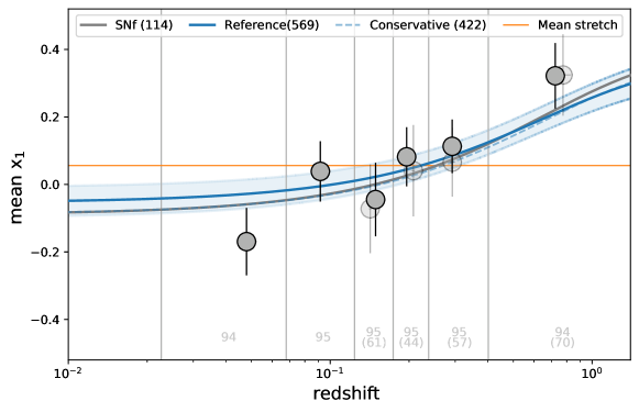
Figure 6: Evolution of the mean SN SALT2.4 stretch ($x_{1}$) as a function of redshift. Markers show the stretch plain mean (the error is estimated from the scatter) measured in redshift bins of equal sample size, indicated in light gray at the bottom of each redshift bin. Full and light markers are used when the fiducial or conservative samples are considered, respectively. The horizontal orange line represents the mean stretch for the nonevolving Gaussian model (last line of Table 3) on the fiducial sample. Best fits of our base drifting model are shown as blue, dashed blue, and gray when fitted on the fiducial sample, the conservative sample, or the SNfactory dataset only, respectively; all are compatible. The light blue band illustrates the amplitude of the error (including covariance) of the best-fit model when considering the fiducial dataset.

3.3 Alternative models

In Section 3.1 we have modeled the underlying stretch distribution following Rigault et al. (2020), that is, as a single Gaussian for the young SNe Ia and a mixture of two Gaussians for the old SNe Ia population, one being the same as for the young population, plus another one for the fast-declining SNe Ia that appear to only exist in old local environments. This is our so-called base model. However, to test different modeling choices, we implemented a suite of alternative parameterizations that we also adjusted to the data following the procedure described in Section 3.2.2.

Howell et al. (2007) used a simpler unimodal model per age category, assuming a single normal distribution for each of the young and old populations. We thus considered a Howell+drift model, with one single Gaussian per age group and the $\delta(z)$ drift from Eq. 1.

Alternatively, because we aim to probe the existence of an evolution with redshift, we also tested constant models by restricting the base and Howell models to use an assumed redshift-independent fraction $\delta(z)\equiv f$ of young SNe; these models are hereafter labeled base+constant and Howell+constant.

We also considered another intrinsically nondrifting model, the functional form developed for beams with bias correction (BBC, Scolnic & Kessler, 2016; Kessler & Scolnic, 2017), used in recent SN cosmological analyses (e.g., Scolnic et al., 2018; Abbott et al., 2019; Riess et al., 2016, 2019) to account for Malmquist biases. The BBC formalism assumes sample-based (hence intrinsically nondrifting) asymmetric Gaussian stretch distributions: $\mathcal{N}\left(\mu,\sigma_{-}{}^{2}\;\text{if}\;x_{1}<\mu,\;\text{else}\;\sigma_{+}{}^{2}\right)$. The idea behind this sample-based approach is twofold: (1) Malmquist biases are driven by survey properties, and (2) because current surveys cover limited redshift ranges, having a sample-based approach covers some potential redshift evolution information (Scolnic & Kessler, 2016; Scolnic et al., 2018). See a more detailed discussion of BBC in Section 5. Finally, for the sake of completeness, we also considered redshift-independent pure and asymmetric Gaussian models.

4 Results

We adjusted each of the models described above on both the fiducial and conservative samples (cf. Section 2). The results are gathered in Table 3 and are illustrated in Fig. 7.

Table 3: Comparison of the relative ability of each model to describe the data. For each considered model, we report whether the model is drifting, its number of free parameters, and for both the fiducial and the conservative cuts, $-2\ln(L)$ (see Eq. 4), the AIC and the AIC difference ($\Delta$AIC) between this model and the base model used as reference because it has the lowest AIC.

			Fiducial sample (569 SNe)			Conservative sample (422 SNe)
Name	drift	$k$	$-2\ln(L)$	AIC	$\Delta$AIC	$-2\ln(L)$	AIC	$\Delta$AIC
Base	$\delta(z)$	5	1456.7	1466.7	–	1079.5	1089.5	–
Howell+drift	$\delta(z)$	4	1463.3	1471.3	$-4.6$	1088.2	1096.2	$-6.7$
Asymmetric	–	3	1485.2	1491.2	$-24.5$	1101.3	1107.3	$-17.8$
Howell+const	$f$	5	1484.2	1494.2	$-27.5$	1101.2	1111.2	$-21.7$
Base+const	$f$	6	1484.2	1496.2	$-29.5$	1101.2	1113.2	$-23.7$
Per sample Asym.	per sample	3$\times$5	1468.2	1498.2	$-31.5$	1083.6	1113.6	$-24.1$
Gaussian	–	2	1521.8	1525.8	$-59.1$	1142.6	1146.6	$-57.1$

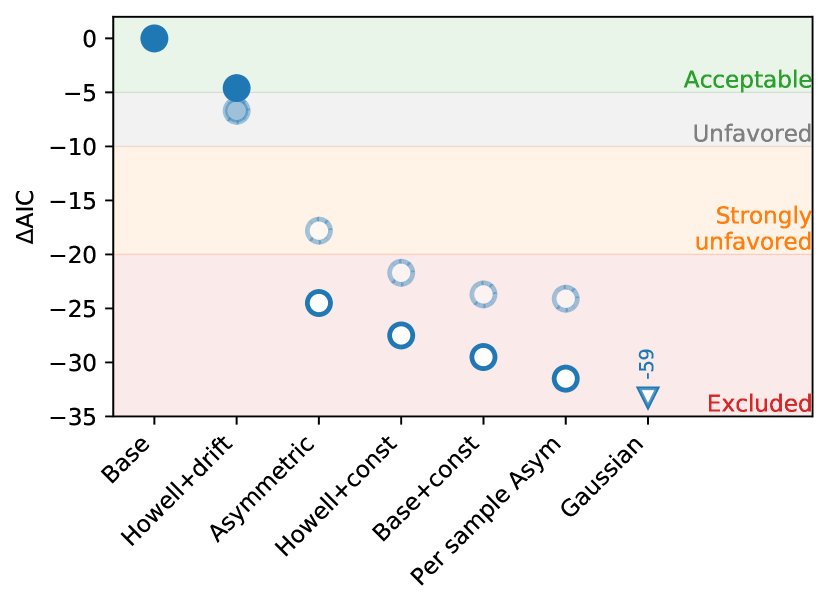
Figure 7: $\Delta$AIC between base model (reference) and other models (see Table 3). Full and open blue markers correspond to models with and without redshift drift, respectively. Light markers show the results when the analysis is performed on the conservative sample rather than the fiducial one. Color bands illustrate the validity of the models, from acceptable ($\Delta\mathrm{AIC}>-5$) to excluded ($\Delta\mathrm{AIC}<-20$), see text. According to the AIC, all nondrifting models (open symbols) are excluded as a poorer representation of the data than the base (drifting) model.

Because the various models have different degrees of freedom, we used the Akaike information criterion (AIC, e.g., Burnham & Anderson, 2004) to compare their ability to properly describe the observations. This estimator penalizes additional degrees of freedom to avoid overfitting the data and is defined as follows:

$$\mathrm{AIC}=-2\ln(L)+2k,$$ (5)

where $-2\ln(L)$ is derived by minimizing Eq. (4), and $k$ is the number of free parameters to be adjusted. The reference model has the smallest AIC; in comparison to this model, the models with $\Delta\mathrm{AIC}<5$ are coined acceptable, those with $5<\Delta\mathrm{AIC}<20$ are not favored, and those with $\Delta\mathrm{AIC}>20$ are deemed excluded. This roughly corresponds to 2, 3, and 5 $\sigma$ limits for a Gaussian probability distribution.

The best model (with the smallest AIC) is the so-called base model and thus is our reference model; this is true for the fiducial and conservative samples. The base model also has the smallest $-2\ln(L)$, making it the most likely model even when the overfitting issue that is accounted for by the AIC formalism is ignored.

Furthermore, we find that redshift-independent stretch distributions are all excluded as suitable descriptions of the data relative to the base model. The best nondrifting model (the asymmetric model) has a very marginal chance ($p\equiv\exp\left(\Delta\mathrm{AIC}/2\right)=5\times 10^{-6}$) to describe the data as well as the base model. This result is just a quantitative assessment of qualitative facts that are clearly visible in Fig. 6: The mean SN stretch per bin of redshift strongly suggests a significant redshift evolution rather than a constant value, and this evolution is well described by Eq. 1.

Surprisingly, the sample-based Gaussian asymmetric modeling used by current implementations of the BBC technique (Scolnic & Kessler, 2016; Kessler & Scolnic, 2017) has one of the highest AIC values in our analysis (see Section 4). While its $-2\ln(L)$ is the smallest of all redshift-independent models (but still $-11.5$ lower than the reference base model), it is strongly penalized for requiring 15 free parameters ($\mu_{0},\sigma_{\pm}$ for each of the five samples of the analysis). Hence, its $\Delta\mathrm{AIC}<-20$, which could be interpreted as a probability $p=2\times 10^{-7}$ of being as good a representation of the data as the base model.

We note that when models are compared that were adjusted on individual subsamples rather than globally, the Bayesian information criterion ($\mathrm{BIC}=-2\ln(L)+k\ln(n)$, with $n$ the number of data points) might be better suited than AIC because it explicitly accounts for the fact that each subsample is fitted separately: the sample-based model BIC is rightfully the sum of the BIC for each sample. We find $\Delta\mathrm{BIC}=-48$, again refuting the sample-based asymmetric Gaussian model as being as pertinent as the base model.

In order to ensure that our results are not driven by the incompletely modeled HST subsample, we recomputed $\Delta$AIC for each model excluding this dataset; this did not change $\Delta$AIC by more than few tenths. The consistency of these values with those in Table 3 shows that the HST subsample does not drive our conclusions.

We report in Table 4 our determination of $\mu_{0}$ and $\sigma_{\pm}$ for each sample when an asymmetric Gaussian model was implemented, and adjusted on the nominally selection-free samples using our fiducial cuts (see Section 2). Our results are in close agreement with those of Scolnic & Kessler (2016) for the SNLS and SDSS and with the results reported by Scolnic et al. (2018) for PS1, who derived these model parameters using the full BBC formalism, using numerous simulations to model the observational selection effects (see details, e.g., Section 3 of Kessler & Scolnic 2017). The agreement between our fit of the asymmetric Gaussians on the supposedly selection-free part of the samples and the results derived using the BBC formalism supports our approach to constructing a sample with negligible observational selection effects. If we were to use the Scolnic & Kessler (2016) and Scolnic et al. (2018) best-fit values of the $\mu_{0},\sigma_{\pm}$ asymmetric parameters for the SNLS, SDSS and PS1, respectively, the $\Delta$AIC between our base drifting model and the BBC modeling would go even deeper from $-32$ to $-47$. We further discuss the consequence of this result for cosmology in Section 5.

Table 4: Best-fit parameters for our sample-based asymmetric modeling of the underlying stretch distribution.

Asymmetric	$\sigma_{-}$	$\sigma_{+}$	$\mu_{0}$
SNfactory	1.34 $\pm$ 0.13	0.41 $\pm$ 0.10	0.68 $\pm$ 0.15
SDSS	1.31 $\pm$ 0.11	0.42 $\pm$ 0.09	0.72 $\pm$ 0.13
PS1	1.01 $\pm$ 0.11	0.52 $\pm$ 0.12	0.38 $\pm$ 0.16
SNLS	1.41 $\pm$ 0.13	0.15 $\pm$ 0.13	1.22 $\pm$ 0.15
HST	0.76 $\pm$ 0.36	0.79 $\pm$ 0.35	0.11 $\pm$ 0.44

We also performed tests allowing the high-stretch mode of the old population to differ from the young population mode, hence adding two degrees of freedom. The corresponding fit is not significantly better, with a $\Delta$AIC of $-0.4$. This reinforces our assumption that the young and old populations indeed appear to share the same underlying high-stretch mode. Furthermore, we might wonder whether a low-stretch mode might also exist in the young population (see Fig. 5). We tested for this by allowing this population to also be bimodal, finding the amplitude of such a low-stretch mode to be compatible with 0 ($<2\%$) in this young population. More generally, this raises the question of how well a given environmental tracer (here LsSFR) traces the age. An analysis dedicated to this question will be presented in Briday et al. in prep.

Finally, ignoring the LsSFR measurements, which are only available for the SNfactory dataset (see Section 3), reduces the significance of the results presented in this section, as expected. Even so, nondrifting models remain strongly disfavored. For instance, the best-fitting sample-based Gaussian asymmetric model is still $\Delta\mathrm{AIC}<-10$, which is less representative of the data than our base drifting model.

5 Discussion

To the best of our knowledge, a SN Ia stretch redshift drift modeling has never been explicitly used in cosmological analyses, although a Bayesian hierarchy formalism such as UNITY (Rubin et al., 2015), BAHAMAS (Shariff et al., 2016), or Steve (Hinton et al., 2019) can easily allow it (see, e.g., sections 1.3 and 2.5 of Rubin et al. (2015)). Not doing so is a second-order issue for SN cosmology because it only affects the way in which the Malmquist bias is accounted for. As long as the Phillips relation (Phillips, 1993) standardization parameter $\alpha$ is not redshift dependent (a study that is beyond the scope of this paper, but see, e.g., Scolnic et al. 2018), the stretch-corrected SNe Ia magnitudes used for cosmology are indeed blind to the underlying stretch distribution for complete samples. However, surveys usually do have significant Malmquist bias for the upper half of their SN redshift distribution. As a consequence, mismodeling of the underlying stretch distribution will bias the SN magnitudes derived from such surveys.

Commonly used Malmquist bias correction techniques, such as the BBC-formalism, assume per-sample asymmetric Gaussian functions to model the underlying stretch and color distributions. As shown in Section 4, however, such a sample-based distribution is excluded in comparison to our drifting model. In contrast to what Scolnic & Kessler (2016, Section 2) and Scolnic et al. (2018, Section 5.4) have suggested, that is, that traditional surveys span sufficiently limited redshift ranges such that the per-sample approach accounts for implicit redshift drifts, a direct modeling of the redshift drift is therefore more appropriate than a sample-based approach. We add here that as measurements of modern surveys try to cover increasingly larger redshift ranges in order to reduce calibration systematic uncertainties, this sample-based approach becomes less valid, notably for PS1, DES and, soon, the Large Synoptic Survey Telescope.

We illustrate in Fig. 8 the prediction difference in the underlying stretch distribution between the per-sample asymmetric modeling and our base drifting model for the PS1 sample. Our model is bimodal, and the relative amplitude of each mode depends on the redshift-dependent fraction of old and young SNe Ia in the sample: the higher the fraction of old SNe Ia (at lower redshift), the higher the amplitude of the old-specific low-stretch mode. This redshift dependence on the underlying stretch distributions is shown with colors from blue to red in Fig. 8 for the redshift range covered by PS1. The observed $x_{1}$ histogram follows the model we defined using the sum of individual underlying SN-redshift distributions. As expected, the two modeling approaches differ mostly in the negative part of the SN stretch distribution. The asymmetric Gaussian distribution goes through the middle of the bimodal distribution, overestimating the number of SNe Ia at $x_{1}\sim-0.7$ and underestimating it at $x_{1}\sim-1.7$ in comparison to our base drifting model for typical PS1 SN redshifts. This means that the SN bias-corrected standardized magnitude estimated at a redshift plagued by observational selection effects would be biased by a mismodeling of the true underlying stretch distribution.

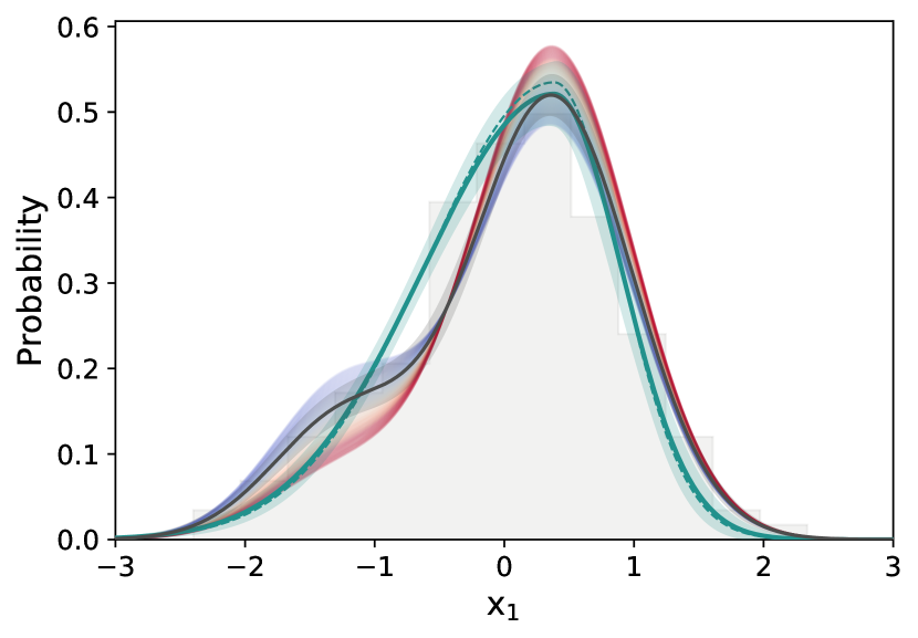
Figure 8: Distribution of the PS1 SN Ia SALT2.4 stretch ($x_{1}$) after the fiducial redshift limit cut (gray histogram). This distribution is supposed to be a random draw from the underlying stretch distribution. The green lines show the BBC model of this underlying distribution (asymmetric Gaussian). The full line (band) is our best fit (its error); the dashed line shows the Scolnic et al. (2018) result. The black line (band) shows our best-fit base modeling (its error, see Table 2) that includes redshift drift. For illustration, we show (colored from blue to red with increasing redshifts) the evolution of the underlying stretch distribution as a function of redshift for the redshift range covered by PS1 data.

Assessing the amplitude of this magnitude bias for cosmology is beyond the scope of this paper given the complexity of the BBC analysis. It would require a full study using our base model (Eq. 3.1) in place of the sample-based asymmetric modeling as part of the BBC simulations. However, we already highlighted that even if a nondrifting sample-based model could provide comparable result in the volume-limited part of the various samples, these models would differ when extrapolated to higher redshifts, precisely where the underlying distribution will matter for correcting Malmquist biases.

In the era of modern cosmology, where we aim to measure $w_{0}$ at a subpercent level and $w_{a}$ with 10% precision (e.g., Ivezić et al., 2019), we stress that correct modeling of potential SN redshift drift should be further studied and care should be taken when samples are used that are affected by observational selection effects.

6 Conclusion

We have presented an initial study of the drift of the underlying SNe Ia stretch distribution as a function of redshift. We built effectively volume-limited SN Ia subsamples from the Pantheon dataset (Scolnic et al., 2018, SDSS, PS1, and SNLS), to which we added HST and SNfactory data from Rigault et al. (2020) for the high- and low-redshift bins. We only considered the SNe that have been discovered in the redshift range of each survey in which observational selection effects are negligible, so that the observed SNe Ia stretches are a random sampling of the true underlying distribution. This resulted in a fiducial sample of 569 SNe Ia (422 SNe when more conservative cuts were applied).

Following predictions made in Rigault et al. (2020), we introduced a redshift drift model that depends on the expected fraction of young and old SNe Ia as a function of redshift, with each age population having its own underlying stretch distribution.

In addition to this base model, we studied various distributions, including redshift-independent models; we also studied the prediction from a per-sample asymmetric Gaussian stretch distribution used, for instance, by the beams with bias correction Malmquist bias correction algorithm (Scolnic & Kessler, 2016; Kessler & Scolnic, 2017). Our conclusions are listed below.

1. The underlying SN Ia stretch distribution is significantly redshift dependent, as previously suggested by Howell et al. (2007), for example, in a way that observational selection effects alone cannot explain. This result is largely independent of the details of each age-population model.

2. Redshift-independent models are quantitatively excluded as suitable descriptions of the data relative to our base model. This model assumes that (1) the younger population has a unimodal Gaussian stretch distribution while the older population stretch distribution is bimodal, one mode being the same as the young one, and (2) the evolution of the relative fraction of younger and older SNe Ia follows the prediction made in Rigault et al. (2020). This second result further supports the existence of both young and old SN Ia populations, in agreement with rate studies (Mannucci et al., 2005; Scannapieco & Bildsten, 2005; Sullivan et al., 2006; Aubourg et al., 2008).

3. Models using survey-based asymmetric Gaussian distributions, for instance, as employed in the current implementation of BBC, are excluded as a good description of the data relative to our drifting model. This means that the sample-based approach does not accurately account for redshift drift, a problem that will be exacerbated as surveys span increasingly larger redshift ranges. As a result, even if the necessary extra degrees of freedom might be acceptable given the large number of SNe Ia in cosmological studies, extrapolating the SN property distributions from the volume-limited part of a survey to its Malmquist-biased magnitude-limited part would still be inaccurate because of the redshift evolution.

4. Given the current dataset, we suggest the use of the following stretch population model as a function of redshift:

   $$X_{1}\left(z\right)=\delta(z) \times\mathcal{N}(\mu_{1},\sigma_{1}{}^{2})\,+$$

   $$(1-\delta(z)) \times\left[a\times\mathcal{N}(\mu_{1},\sigma_{1}{}^{2})+(1-a)\times\mathcal{N}(\mu_{2},\sigma_{2}{}^{2})\right],$$ (3.1)

   with $a=0.51$, $\mu_{1}=0.37$, $\mu_{2}=-1.22$, $\sigma_{1}=0.61$, and $\sigma_{2}=0.56$ (see Table 2), and using the age-population drift model,

   $$\delta(z) =\left(K^{-1}\times(1+z)^{-2.8}+1\right)^{-1}$$ (1)

   with $K=0.87$.

We considered a simple two-population Gaussian mixture modeling. Additional data free from significant Malmquist bias would enable us to refine it as required. We note that samples at the low- and high-redshift ends of the Hubble diagram would be particularly helpful for this drifting analysis; fortunately, this will soon be provided by the Zwicky Transient Facility (low-$z$, Bellm et al., 2019; Graham et al., 2019) and the Subaru and SeeChange SNe Ia programs (high-$z$), respectively.

The next step in this line of analysis will incorporate our model into the SNANA framework (Kessler et al., 2009), both to more accurately account for observational selection functions and to test the effect of our model on the derivation of cosmological parameters. This study is currently being conducted.