The semi-hierarchical Dirichlet Process and its application to clustering homogeneous distributions

Abstract

Assessing homogeneity of distributions is an old problem that has received considerable attention, especially in the nonparametric Bayesian literature. To this effect, we propose the semi-hierarchical Dirichlet process, a novel hierarchical prior that extends the hierarchical Dirichlet process of Teh et al. (2006) and that avoids the degeneracy issues of nested processes recently described by Camerlenghi et al. (2019a). We go beyond the simple yes/no answer to the homogeneity question and embed the proposed prior in a random partition model; this procedure allows us to give a more comprehensive response to the above question and in fact find groups of populations that are internally homogeneous when $I\geq 2$ such populations are considered. We study theoretical properties of the semi-hierarchical Dirichlet process and of the Bayes factor for the homogeneity test when $I=2$. Extensive simulation studies and applications to educational data are also discussed.

1 Introduction

The study and development of random probability measures in models that take into account the notion of data that are not fully exchangeable has sparked considerable interest in the Bayesian nonparametric literature. We consider here the notion of partial exchangeability in the sense of de Finetti (see de Finetti, 1938; Diaconis, 1988), which straightforwardly generalized the notion of an exchangeable sequence of random variables to the case of invariance under a restricted class of permutations. See also Camerlenghi et al. (2017) and references therein. In particular, our focus is on assessing whether two or more populations (or groups) of random variables can be considered exchangeable rather than partially exchangeable, that is whether they arose from a common population/random distribution or not.

To be mathematically accurate, let us introduce partial exchangeability for a sequence of random variables. Let $\mathbb{Y}$ denote a complete and separable metric space (i.e. a Polish space) with corresponding metric $d$. Let $\mathcal{Y}$ denote the Borel $\sigma$-algebra of $\mathbb{Y}$, and $\mathbb{P}_{\mathbb{Y}}$ denote the space of all probability measures on $(\mathbb{Y},\mathcal{Y})$, with Borel $\sigma$-algebra $\mathcal{P}_{\mathbb{Y}}$. We will often skip reference to $\sigma$-algebras. A double sequence $(y_{11},y_{12},y_{13},\ldots,y_{21},y_{22},y_{23},\ldots)$ of $\mathbb{Y}$-valued random variables, defined on a probability space $(\Omega,\mathcal{F},P)$ is called partially exchangeable if for all $n,m\geq 1$ and all permutations $(i(1),\ldots,i(n))$ and $(j(1),\ldots,j(m))$ of $(1,\ldots,n)$ and $(1,\ldots,m)$ respectively, we have

$$\mathcal{L}(y_{11},\ldots,y_{1n},y_{21},\ldots,y_{2m})=\mathcal{L}(y_{1i(1)},\ldots,y_{1i(n)},y_{2j(1)},\ldots,y_{2j(m)}).$$

Partial exchangeability can thus be conceptualized as invariance of the joint law above under the class of all permutations acting on the indices within each of the samples. Here and from now on, the distribution of a random element $y$ is denoted by $\mathcal{L}(y)$.

The previous setting can be immediately extended to the case of $I$ different populations or groups. By de Finetti’s representation theorem (see the proof in Regazzini, 1991), partial exchangeability for the array of $I$ sequences of random variables $(y_{11},y_{12},\ldots,y_{21},y_{22},\ldots$, $y_{I1},y_{I2},\ldots)$ is equivalent to

$$P(y_{ij}\in A_{ij},\,j=1,\ldots,N_{i},\,i=1,\ldots,I)=\int_{\mathbb{P}_{\mathbb{Y}}^{I}}\prod_{i=1}^{I}\prod_{j=1}^{N_{i}}p_{i}(A_{ij})\,Q(dp_{1},\ldots,dp_{I}),$$

for any $N_{1},\ldots,N_{I}\geq 1$ and Borel sets $\{A_{ij}\}$ for $j=1,\ldots,N_{i}$ and $i=1,\ldots,I$. In this case, de Finetti’s measure $Q$ is defined on the $I$-fold product space $\mathbb{P}_{\mathbb{Y}}^{I}=\mathbb{P}_{\mathbb{Y}}\times\mathbb{P}_{\mathbb{Y}}\times\cdots\times\mathbb{P}_{\mathbb{Y}}$, and $(p_{1},p_{2},\ldots,p_{I})\sim Q$. The whole joint sequence of random variables is exchangeable if and only if $Q$ gives probability 1 to the measurable set $S=\{(p_{1},p_{2},\ldots,p_{I})\in\mathbb{P}_{\mathbb{Y}}^{I}:\,p_{1}=p_{2}=\cdots=p_{I}\}$.

Hence, partial exchangeability of data from different groups (or related studies) is a convenient context to analyze departures from exchangeability. While homogeneity of groups here amounts to full exchangeability, departures from this case may follow different directions, including independence of the population distributions $p_{1},p_{2},\ldots,p_{I}$. However it could be interesting to investigate other types of departures from exchangeability beyond independence. The main goal here is to build a prior $Q$ for $(p_{1},p_{2},\ldots,p_{I})$ that is able to capture a wider range of different behaviors, not only restricting the analysis to assessing equality or independence among $p_{1},p_{2},\ldots,p_{I}$. In the simplest case of $I=2$, we just compare two distributions/populations, but we aim here at extending this notion to $I>2$ groups. In particular, we address the following issue: if the answer to the question of homogeneity within all these groups is negative, a natural question immediately arises, namely, can we assess the existence of homogeneity within certain populations? In other words, we would like to find clusters of internally homogeneous populations.

Vectors of dependent random distributions appeared first in Cifarelli and Regazzini (1978), but it was in MacEachern (1999) where a large class of dependent Dirichlet processes was introduced, incorporating dependence on covariates through the atoms and/or weights of the stick-breaking representation. Following this line, De Iorio et al. (2004) proposed an ANOVA-type dependence for the atoms. These last two papers have generated an intense stream of research which is not our focus here. For a review of such constructions, see Quintana et al. (2020).

Our approach instead constructs a prior that explicitly considers a departure from exchangeability. Other authors have considered similar problems. Müller et al. (2004) and Lijoi et al. (2014a) constructed priors for the population distributions by these distributions with the addition of a common component. See also Hatjispyros et al. (2011), Hatjispyros et al. (2016) and Hatjispyros et al. (2018) for related models with increasing level of generalization. Several references where the focus is on testing homogeneity across groups of observations are available. Ma and Wong (2011) and Soriano and Ma (2017) propose the coupling optional Pólya tree prior, which jointly generates two dependent random distributions through a random-partition-and-assignment procedure similar to Pólya trees. The former paper consider both testing hypotheses from a global point of view, while the latter takes a local perspective on the two-sample hypothesis, detecting high resolution local differences. Bhattacharya and Dunson (2012) propose a Dirichlet process (DP) mixture model for testing whether there is a difference in distributions between groups of observations on a manifold. Both Chen and Hanson (2014) and Holmes et al. (2015) consider the two-sample testing problem, using a Pólya tree prior for the common distribution in the null, while the model for the alternative hypothesis assumes that the two population distributions are independent draws from the same Pólya tree prior. Their approaches differ in the way they specify the Pólya tree prior. Gutiérrez et al. (2019) consider a related problem, where a Bayesian nonparametric strategy to test for differences between a control group and several treatment regimes is proposed. Pereira et al. (2020) extend this idea to testing equality of distributions of paired samples, with a model for the joint distribution of both samples defined as a mixture of DPs with a spike-and-slab prior specification for its base measure.

Another traditional (and fruitful) approach for modeling data arising from a collection of groups or related studies involves the construction of hierarchical random prior probability measures. One of the first such examples in the BNP literature, is the well-known hierarchical DP mixtures introduced in Teh et al. (2006). Generalizations beyond the DP case are currently an active area of research, as testified by a series of recent papers dealing with various such hierarchical constructions; these include Camerlenghi et al. (2019b), Argiento et al. (2019) and Bassetti et al. (2019). See the discussion below.

Our first contribution is the introduction of a novel class of nonparametric priors that, just as discussed in Camerlenghi et al. (2019a), avoids the degeneracy issue of the nested Dirichlet process (NDP) of Rodríguez et al. (2008) that arises from the presence of shared atoms across populations. Indeed, Camerlenghi et al. (2019a) showed that under the NDP, if two populations share at least one common latent variable in the mixture model, then the model identifies the corresponding distributions as completely equal. To overcome the degeneracy issue, they resort to a latent nested construction in terms of normalized random measures that adds a shared random measure to draws from the NDP. Instead, we use a variation of the hierarchical DP (HDP), that we term the semi-HDP, but where the baseline distribution is itself a mixture of a DP and a non-atomic measure. We will show that this procedure solves the degeneracy problem as well. While relying on a different model, Lijoi et al. (2020a) also propose to build on the HDP, combining it with the NDP, to overcome the degeneracy issue of nested processes.

Our second contribution is that the proposed model overcomes some of the practical and applied limitations of the latent nested approach by Camerlenghi et al. (2019a). As pointed out in Beraha and Guglielmi (2019), the latent nested approach becomes computationally burdensome in the case of $I>2$ populations. In contrast, implementing posterior inference for the semi-HDP prior does not require restrictions on $I$. We discuss in detail how to carry out posterior inference in the context of hierarchical models based on the semi-HDP.

A third contribution of this article is that we combine the proposed semi-HDP prior with a random partition model that allows different populations to be grouped in clusters that are internally homogeneous, i.e. arising from the same distribution. See an early discussion of this idea in the context of contingency tables in Quintana (1998). The far more general extension we aim for here is also useful from the applied viewpoint of finding out which, if any, of the $I$ populations are internally homogeneous when homogeneity of the whole set does not hold. For the purpose of assessing global exchangeability, one may resort to discrepancy measures (Gelman et al., 1996); see also Catalano et al. (2021). In our approach, homogeneity corresponds to a point-null hypothesis about a discrete vector parameter, as we adopt a “larger” model for the alternative hypothesis within which homogeneity is nested. We discuss the specific case of adopting Bayes factors for the proposed test within the partial exchangeability framework. We show that the Bayes factor for this test is immediately available, and derive some of its theoretical properties.

The rest of this article is organized as follows. Section 2 gives some additional background that is relevant for later developments, presents the semi-HDP prior (Section 2.2) and, in particular, it describes a food court of Chinese restaurants with private and shared areas metaphor (Section 2.3). Section 3 studies several theoretical properties of the semi-HDP such as support, moments, the corresponding partially exchangeable partition probability function (in a particular case) and specially how the degeneracy issue is overcome under this setting. Section 3.3 specializes the discussion to the related issue of testing homogeneity when $I=2$ populations are present, and we study properties of the Bayes Factor for this test. Section 4 describes a computational strategy to implement posterior inference for the class of hierarchical models based on our proposed semi-HDP prior. Extensive simulations, with $I=2$, $4$ and $100$ populations are presented in Section 5. An application to an educational data set is discussed in Section 6. The article concludes with a discussion in Section 7. An appendix collects the proofs for the theoretical results and a discussion on consistency for the Bayes Factor in the case of $I=2$ homogeneous populations. Code for posterior inference has been implemented in C++ and is available as part of the BayesMix library.

2 Assessing Exchangeability within a Partially Exchangeable Framework

While exchangeability can be explored in more generality, for clarity of exposition we set up our discussion in the context of continuous univariate responses, but extensions to, e.g. multivariate responses, can be straightforwardly accommodated in our framework.

2.1 A common home for exchangeability and partial exchangeability

A flexible nonparametric model for each group can be constructed by assuming a mixture, where the mixing group-specific distribution $G_{i}$ is a random discrete probability measure (r.p.m.), i.e.

$$y_{ij}\,|\,G_{i}\stackrel{{\scriptstyle\mbox{\scriptsize iid}}}{{\sim}}p_{i}(\cdot)=\int_{\Theta}k(\cdot\,|\,\theta)\,G_{i}(d\theta),\qquad j=1,\ldots,N_{i},$$ (1)

where $k(\cdot\,|\,\theta)$ is a density in $\mathbb{Y}$ for any $\theta\in\Theta$, and $G_{i}$ is, for example, a DP on $\Theta$. Note that, with a little abuse of notation, $p_{i}$ in (1) and in the rest of the paper denotes the conditional population density of group $i$ (before $p_{i}$ represented the population distribution of group $i$ in de Finetti’s theorem). In what follows, we will always assume that the parametric space is contained in $\mathbb{R}^{p}$ for some positive integer $p$, and we will always assume the Borel $\sigma$–field $\mathcal{B}(\Theta)$ of $\Theta$. Using the well-known alternative representation of the mixture in terms of latent variables, the previous expression is equivalent to assuming that for any $i$,

$$y_{ij}\,|\,\theta_{ij}\stackrel{{\scriptstyle\mbox{\scriptsize ind}}}{{\sim}}k(\cdot\,|\,\theta_{ij}),\quad\theta_{ij}\,|\,G_{i}\stackrel{{\scriptstyle\mbox{\scriptsize iid}}}{{\sim}}G_{i},\quad j=1,\ldots,N_{i}.$$ (2)

In this case, partial exchangeability of observations $(y_{ij})_{ij}$ is equivalent to partial exchangeability of the latent variables $(\theta_{ij})_{ij}$. Hence exchangeability of observations $(y_{ij})_{ij}$ is equivalent to the statement $G_{1}=G_{2}=\cdots=G_{I}$ with probability one.

In the next subsection we develop one of the main contributions of this paper, namely, the construction of a prior distribution $\pi(G_{1},\ldots,G_{I})$ such that there is positive prior probability that $G_{1}=G_{2}=\cdots=G_{I}$, but avoiding the degeneracy issues discussed in Camerlenghi et al. (2019a) and that would arise if we assumed that $(G_{1},\ldots,G_{I})$ were distributed as the NDP by Rodríguez et al. (2008). Briefly, $(G_{1},\ldots,G_{I})$ is distributed as the NDP if

$$G_{i}\,|\,G\stackrel{{\scriptstyle\mbox{\scriptsize iid}}}{{\sim}}G=\sum_{\ell=1}^{\infty}\pi_{\ell}\delta_{G^{*}_{\ell}},\quad i=1,\ldots,I\quad\text{and}\quad G^{*}_{\ell}\stackrel{{\scriptstyle\mbox{\scriptsize iid}}}{{\sim}}Q_{0}=\mathcal{D}_{\gamma G_{00}},$$

i.e., the independent atoms in $G$ are all drawn from a DP on $\Theta$, specifically $G^{*}_{\ell}=\sum_{h=1}^{\infty}w_{h\ell}\delta_{\theta_{h\ell}}$, with $\theta_{h\ell}\stackrel{{\scriptstyle\mbox{\scriptsize iid}}}{{\sim}}G_{00}$, a probability measure on $\Theta$, and $\alpha,\gamma>0$. The weights $(\pi_{j})_{j}$ and $(w_{h\ell})_{h}$, $\ell=1,2,\ldots$, are independently obtained from the usual stick-breaking construction, with parameters $\alpha$ and $\gamma$, respectively. Here $\mathcal{D}_{\gamma G_{00}}$ denotes the Dirichlet measure, i.e. the distribution of a r.p.m. that is a DP with measure parameter $\gamma G_{00}$. However, nesting discrete random probability measures produces degeneracy to the exchangeable case. As mentioned in Section 1, Camerlenghi et al. (2019a) showed that the posterior distribution degenerates to the exchangeable case whenever a shared component is detected, i.e., the NDP does not allow for sharing clusters among non-homogeneous populations. The problem is shown to affect any construction that uses nesting, and not just the NDP.

To overcome the degeneracy issue, while retaining flexibility, Camerlenghi et al. (2019a) proposed the so-called Latent Nested Nonparametric priors. These models involve a shared random measure that is added to the draws from a Nested Random Measure, hence accommodating for shared atoms. See also the discussion by Beraha and Guglielmi (2019). There are two key ideas in their model: ($i$) nesting discrete random probability measures as in the case of the NDP, and ($ii$) contaminating the population distributions with a common component as in Müller et al. (2004) and also, Lijoi et al. (2014b). The contamination aspect of the model yields dependence among population-specific random probability measures, and avoids the degeneracy issue pointed out by the authors, while the former accounts for testing homogeneity in multiple-sample problems. Their approach, however, becomes computationally burdensome in the case of $I>2$ populations, and it is not clear how to extend their construction to allow for the desired additional analysis, i.e. assessing which, if any, of the $I$ populations are internally homogeneous when homogeneity of the whole set does not hold.

2.2 The Model

We present now a hierarchical model that allows us to assess homogeneity, while avoiding the undesired degeneracy issues and which further enables us to construct a grouping of populations that are internally homogeneous. To do so we create a hierarchical representation of distributions that emulates the behavior arising from an exchangeable partition probability function (EPPF; Pitman, 2006) such as the Pólya urn. But the main difference with previous proposals to overcome degeneracy is that we now allow for different populations to arise from the same distribution, while simultaneously incorporating an additional mechanism for populations to explicitly differ from each other.

Denote $[I]=\{1,\ldots,I\}$. A partition $S_{1},\ldots,S_{k}$ of $[I]$ can be described by cluster assignment indicators $\mbox{\boldmath{$c$}}=(c_{1},\ldots,c_{I})$ with $c_{i}=\ell$ iff $i\in S_{\ell}$. Assume this partition arises from a given EPPF. We introduce the following model for the latent variables in a mixture model such as (2). Let $\mbox{\boldmath{$y$}}_{i}:=(y_{i1},\ldots,y_{iN_{i}})$, for $i=1,\ldots,I$. We assume that $\mbox{\boldmath{$y$}}_{1},\ldots,\mbox{\boldmath{$y$}}_{I}$, given all the population distributions $F_{1},\ldots,F_{I}$ are independent, and furthermore arising from

$$y_{ij}\,|\,F_{1},\dots,F_{I},\mbox{\boldmath{$c$}} \stackrel{{\scriptstyle\mbox{\scriptsize iid}}}{{\sim}}\int_{\Theta}k(\cdot\,|\,\theta)\,F_{c_{i}}(d\theta),\ j=1,\ldots,N_{i},\ \textrm{ for all }i$$ (3)

$$c \sim\pi_{c}(c_{1},\dots,c_{I})$$ (4)

$$F_{1},\dots F_{I}\,|\,\widetilde{P} \stackrel{{\scriptstyle\mbox{\scriptsize iid}}}{{\sim}}\mathcal{D}_{\alpha\widetilde{P}}$$ (5)

$$\widetilde{P} =\kappa G_{0}+(1-\kappa)\widetilde{G}$$ (6)

$$\widetilde{G} \sim\mathcal{D}_{\gamma G_{00}}$$ (7)

$$\kappa \sim Beta(a_{\kappa},b_{\kappa}),$$ (8)

where $\alpha,\gamma>0$. Thus the role of the population mixing distribution $G_{i}$ in (1) – or, equivalently, in (2) – is now played by $F_{c_{i}}$. Observe that $F_{1},\ldots,F_{I}$ in (5) play a role similar to the cluster specific parameters in more standard mixture models. Consider for example a case where $I=4$ and $\mbox{\boldmath{$c$}}=(1,2,3,1)$. Under the above setting, $F_{1},F_{2},F_{3}$ define a model for three different distributions, so that populations 1 and 4 share a common mixing distribution, and $F_{4}$ is never employed.

Equation (5) means that conditionally on $\widetilde{G}$ each $F_{k}$ is an independent draw from a DP prior with mean parameter $\widetilde{P}$ (and total mass $\alpha$), i.e. $F_{k}$ is a discrete r.p.m. on $\Theta\subset\mathbb{R}^{p}$ for some positive integer $p$, with $F_{k}=\sum_{h\geq 1}w_{kh}\delta_{\theta^{*}_{kh}}$ where for any $k$ the weights are independently generated from a stick-breaking process, $\{w_{kh}\}_{h}\stackrel{{\scriptstyle\mbox{\scriptsize iid}}}{{\sim}}SB(\alpha)$, i.e.

$$w_{k1}=\beta_{k1},\quad\ w_{kh}=\beta_{ih}\prod_{j=1}^{h-1}(1-\beta_{kj})\ \ \mbox{for $h=2,3,\ldots$},\quad\beta_{ij}\stackrel{{\scriptstyle\mbox{\scriptsize iid}}}{{\sim}}Beta(1,\alpha),$$

and $\{\theta^{*}_{kh}\}_{h}$, $\{\beta_{kh}\}_{h}$ are independent, with $\theta^{*}_{kh}\,|\,\widetilde{P}\stackrel{{\scriptstyle\mbox{\scriptsize iid}}}{{\sim}}\widetilde{P}$. We assume the centering measure $\widetilde{P}$ in (6) to be a contaminated draw $\widetilde{G}$ from a DP prior, with centering measure $G_{00}$, with a fixed probability measure $G_{0}$. Both $G_{0}$ and $G_{00}$ are assumed to be absolutely continuous (and hence non-atomic) probability measures defined on $\left(\Theta,\mathcal{B}(\Theta)\right)$.

By (7), $\widetilde{G}=\sum_{h\geq 1}p_{h}\delta_{\tau_{h}}$, where $\{p_{h}\}_{h}\sim SB(\gamma)$, $\tau_{h}\stackrel{{\scriptstyle\mbox{\scriptsize iid}}}{{\sim}}G_{00}$ are independent weights and location points. The model definition is completed by specifying $\pi_{c}(c_{1},\dots,c_{I})$. We assume that the $c_{i}$’s are (conditionally) i.i.d. draws from a categorical distribution on $[I]$ with weights $\mbox{\boldmath{$\omega$}}=(\omega_{1},\dots,\omega_{I})$, i.e. $c_{i}\,|\,\mbox{\boldmath{$\omega$}}\stackrel{{\scriptstyle\mbox{\scriptsize iid}}}{{\sim}}Cat([I];\,\mbox{\boldmath{$\omega$}})$, where the elements of $\omega$ are non-negative and constrained to add up to 1. A convenient prior for $\omega$ is a finite dimensional Dirichlet distribution with parameter $\mbox{\boldmath{$\eta$}}=(\eta_{1},\dots\eta_{I})$. Observe that distributions $F_{c_{1}},\ldots,F_{c_{I}}$ allow us to cluster populations, so that there are at most $I$ clusters and consequently $F_{1},\ldots,F_{I}$ are all of the cluster distributions that ever need to be considered.

We say that a vector of random probability measures $(F_{1},\dots,F_{I})$ has the semi-hierarchical Dirichlet process (semi-HDP) distribution if (5)-(7) hold, and we write $(F_{1},\dots,F_{I})\sim semiHDP(\allowbreak\alpha,\gamma,\kappa,G_{0},G_{00})$. It is straightforward to prove that, conditional on $\kappa$ and eventual hyperparameters in $G_{0}$ and $G_{00}$, the expectation of any $F_{i}$ is $\kappa G_{0}+(1-\kappa)G_{00}$ which further reduces to $G_{00}$ if $G_{0}=G_{00}$. Note that $(F_{1},\dots,F_{I})\sim semiHDP(\alpha,\gamma,\kappa,G_{0},G_{00})$ defines an exchangeable prior over a vector of random probability measures.

We note several immediate yet interesting properties of the model. First, note that if $\kappa=1$ in (6), then all the atoms and weights in the representation of the $F_{i}$’s are independent and different with probability one, since the beta distribution and $G_{0}$ are absolutely continuous. If $\kappa=0$, then our prior (5)-(7) coincides with the Hierarchical Dirichlet Process in Teh et al. (2006). Since $\widetilde{G}=\sum_{h\geq 1}p_{h}\delta_{\tau_{h}}$, then, with positive probability, we have $\theta^{*}_{kh}=\theta^{*}_{k^{\prime}m}=\tau_{\ell}$ for $k\neq k^{\prime}$, i.e. all the $F_{k}$’s share the same atoms in the stick-breaking representation of $\widetilde{G}$. However, even when $\kappa=0$, $F_{k}\neq F_{j}$ with probability one, as the weights $\{w_{kh}\}_{h}$ and $\{w_{jh}\}_{h}$ are different, since they are built from (conditionally) independent stick-breaking priors. This is precisely the feature that allows us to circumvent the degeneracy problem.

Second, our model introduces a vector parameter $c$, which assists selecting each population distribution from the finite set $F_{1},\ldots,F_{I}$, in turn assumed to arise from the semi-HDP prior (5)-(7). The former allows two different populations to have the same distribution (or mixing measure) with positive probability, while the latter allows to overcome the degeneracy issue while retaining exchangeability. Indeed, as noted above, $F_{i}$ and $F_{j}$ may share atoms. The atoms in common arise from the atomicity of the base measure and we let the atomic component of the base measure to be a draw from a DP. The result is a very flexible model, that on one hand is particularly well-suited for problems such as density estimation, and on the other, can be used to construct clusters of the $I$ populations, as desired.

2.3 A restaurant representation

To better understand the cluster allocation under model (3)-(7), we rewrite (3) introducing the latent variables $\{\theta_{ij}\}$ as follows

$$y_{ij}\,|\,F_{1},\ldots F_{I},\mbox{\boldmath{$c$}},\theta_{ij} \stackrel{{\scriptstyle\mbox{\scriptsize ind}}}{{\sim}}k(\cdot\,|\,\theta_{ij})$$ (9)

$$\theta_{i1},\ldots\theta_{iN_{i}}\,|\,F_{1},\ldots F_{I},\mbox{\boldmath{$c$}} \stackrel{{\scriptstyle\mbox{\scriptsize iid}}}{{\sim}}F_{c_{i}}$$ (10)

and $\{\theta_{i\ell}\}_{\ell}\perp\{\theta_{jm}\}_{m}$ for $i\neq j$, conditionally on $F_{1},\ldots,F_{I}$.

We first derive the conditional law of the $\theta_{ij}$’s under (9) - (10), and (4)-(6), given $\widetilde{G}$. All customers of group $i$ enter restaurant $r$ (such that $c_{i}=r$). If group $i$ is the first group entering restaurant $r$, then the usual Chinese Restaurant metaphor applies. Instead, let us imagine that group $i$ is the last group entering restaurant $r$ among those such that $c_{m}=r$. Upon entering the restaurant, the customer is presented with the usual Chinese Restaurant Process (CRP), so that

$$\theta_{ij}\,|\,\mbox{\boldmath{$c$}},\{\theta_{mk},\ \forall m:c_{m}=c_{i}=r\},\theta_{i1},\ldots,\theta_{ij-1},\widetilde{G}\\ \sim\sum_{\ell=1}^{H_{r}}\frac{n_{r\ell}}{\alpha+n_{r\boldsymbol{\cdot}}}\delta_{\theta^{*}_{r\ell}}+\frac{\alpha}{\alpha+n_{r\boldsymbol{\cdot}}}\widetilde{P},$$ (11)

that is the CRP when considering all the groups entering restaurant $r$ as a single group. Here $H_{r}$ denotes the number of tables in restaurant $r$, and $n_{r\ell}$ is the number of customers who entered from restaurant $r$ and are seating at table $\ell$. Moreover, note that $\theta^{*}_{r\ell}\,|\,\widetilde{G}\stackrel{{\scriptstyle\mbox{\scriptsize iid}}}{{\sim}}\widetilde{P}$, so that, as in the HDP, there might be ties among the $\theta^{*}_{r\ell}$ also when keeping $r$ fixed. This is an important observation as the fact that there might be ties for different values of $r\neq r^{\prime}$ instead, is exactly what let us avoid the degeneracy to the exchangeable case. Note that (11) holds also for $\theta_{i1}$, i.e. the first customer in group $i$. In the following, we will use clusters or tables interchangeably. However, note that, unlike traditional CRPs, the number of clusters does not coincide with the number of unique values in a sample. This point is clarified in Argiento et al. (2019), who introduce the notion of $\ell$–cluster, which is essentially the table in our restaurant metaphor.

Observe from (11) that when a new cluster is created, its label is sampled from $\widetilde{P}$. In practice, we augment the parameter space with a new binary latent variable for each cluster, namely $h_{r\ell}$, with $h_{r\ell}\stackrel{{\scriptstyle\mbox{\scriptsize iid}}}{{\sim}}\text{Bernoulli}(\kappa)$, so that

$$\theta^{*}_{r\ell}\,|\,h_{r\ell}=1\ \sim G_{0}\qquad\text{ and }\qquad\theta^{*}_{r\ell}\,|\,h_{r\ell}=0,\widetilde{G}\ \sim\widetilde{G}.$$

Upon conditioning on $\{h_{r\ell}\}$ it is straightforward to integrate out $\widetilde{G}$. Indeed, we can write the joint distribution of $\{\theta^{*}_{r\ell},\ \forall r\ \forall\ell\}$, conditional on $\{h_{r\ell}\}$ as

$$\{\theta^{*}_{r\ell}\}\,|\,\{h_{r\ell}\},\widetilde{G}\sim\prod_{r,\ell}G_{0}(d\theta^{*}_{r\ell})^{h_{r\ell}}\ \prod_{r,\ell}\widetilde{G}(d\theta^{*}_{r\ell})^{1-h_{r\ell}}.$$

Hence we see that $\{\theta^{*}_{r\ell},\ \forall r\ \forall\ell:h_{r\ell}=0\}$ is a conditionally i.i.d sample from $\widetilde{G}$ (given all the $h_{rl}$’s and $\widetilde{G}$), so that we can write:

$$\theta^{*}_{r\ell}\,|\,h_{r\ell}=0,\{\theta^{*}_{ij}:h_{ij}=0\}\sim\sum_{k=1}^{H_{0}}\frac{m_{\boldsymbol{\cdot}k}}{m_{\boldsymbol{\cdot}\boldsymbol{\cdot}}+\gamma}\delta_{\tau_{k}}+\frac{\gamma}{m_{\boldsymbol{\cdot}\boldsymbol{\cdot}}+\gamma}G_{00}$$ (12)

and $\tau_{k}\stackrel{{\scriptstyle\mbox{\scriptsize iid}}}{{\sim}}G_{00}$, where $H_{0}$ denotes the number of tables in the common area in Figure 1, and $m_{rk}$ denotes the cardinality of the set $\{\theta^{*}_{r\ell}:\ \theta^{*}_{r\ell}=\tau_{k}\}$. The dot subindex denotes summation over the corresponding subindex values. Hence, conditioning on all the $(r,\ell)$ such that $h_{r\ell}=0$, with $r$ corresponding to a non-empty restaurant, we recover the Chinese Restaurant Franchise (CRF) that describes the HDP.

Figure 1: Restaurant representation of the semi-HDP allocation. In the image, $\mbox{\boldmath{$c$}}=(1,4,1,4)$ so that groups one and three enter in restaurant R1 while groups two and four enter in restaurant R4. In the “common area” two tables are represented, $\tau_{1}$ and $\tau_{2}$. “Zooming” into $\tau_{2}$ shows that there are three different $\theta^{*}$’s associated to the value $\tau_{2}$, namely $\theta^{*}_{12},\theta^{*}_{13}$ and $\theta^{*}_{43}$. The first two originate from R1, showing that it is possible to have ties among the $\theta^{*}$’s even inside the same restaurant, while the table labeled $\theta^{*}_{43}$ shows that it is possible to have ties across different restaurants.

We can describe the previously discussed clustering structure in terms of a restaurant metaphor as the “food court of Chinese restaurants with private and shared areas”. Here, the $\theta^{*}_{r\ell}$ correspond to the tables and $\theta_{ij}$ to the customers. Moreover, a dish is associated to each table. Dishes are represented by the various $\theta^{*}_{r\ell}$’s . There is one big common area where tables are shared among all the restaurants and $I$ additional “private” small rooms, one per restaurant, as seen in Figure 1. The common area accommodates tables arising from the HDP, i.e. those tables such that $\tau_{k}\stackrel{{\scriptstyle\mbox{\scriptsize iid}}}{{\sim}}G_{00}$, while the small rooms host those tables associated to non empty restaurants, such that $\theta^{*}_{r\ell}\,|\,h_{r\ell}=1\stackrel{{\scriptstyle\mbox{\scriptsize iid}}}{{\sim}}G_{0}$. All the customers of group $i$ enter restaurant $r$ (such that $c_{i}=r$). Upon entering the restaurant, a customer is presented with a menu. The $H_{r}$ dishes in the menu are the $\theta^{*}_{r\ell}$’s, and because $\theta^{*}_{r\ell}\stackrel{{\scriptstyle\mbox{\scriptsize iid}}}{{\sim}}\widetilde{P}$, there might be repeated dishes; see (11). The customer either chooses one of the dishes in the menu, with probability proportional to the number of customers who entered the same restaurant and chose that dish, or a new dish (that is not included in the menu yet) with probability proportional to $\alpha$; again, see (11). If the latter option is chosen, with probability $\kappa$ a new table is created in the restaurant-specific area, $H_{r}$ is incremented by one and a new dish $\theta^{*}_{rH_{r}+1}$ is drawn from $G_{0}$. With probability $1-\kappa$ instead, the customer is directed to the shared area, where (s)he chooses to seat in one of the occupied tables with a probability proportional to $m_{\cdot k}$, i.e. the number of items in the menus (from all the restaurants) that are equal to dish $\tau_{k}$, or seats at a new table with a probability proportional to $\gamma$, as seen from (12). We point out that the choice of table in this case is made without any knowledge of which restaurant the dishes came from. Moreover, if the customer chooses to sit at a new table, we increment $H_{0}$ by one and draw $\tau_{H_{0}+1}\sim G_{00}$; we also increment $H_{r}$ by one and set $\theta^{*}_{rH_{r}+1}=\tau_{H_{0}+1}$. Observe that in the original CRF metaphor, it is not the tables that are shared across restaurants, but rather the dishes. In our metaphor instead, we group together all the tables corresponding to the same $\tau_{h}$ and place them in the shared area. This is somewhat reminiscent of the direct sampler scheme for the HDP. Nevertheless, observe that the bookkeeping of the $m_{rk}$’s is still needed. To exemplify this, in Figure 1 we report a “zoom” on a particular shared table $\tau$, showing that the $\theta^{*}$’s associated to that table are still present in our metaphor, but can be collapsed into a single shared table when it is convenient.

3 Theoretical properties of the semi-HDP prior

Here we develop additional properties of the proposed prior model. In particular, we study the topological support of the semi-HDP and show how exactly the degeneracy issue is resolved by studying the induced joint random partition model on the $I$ populations.

3.1 Support and moments

An essential requirement of nonparametric priors is that they should have large topological support; see Ferguson (1973). Let us denote by $\pi_{\mbox{\boldmath{$G$}}}$ the probability measure on $\mathbb{P}_{\Theta}^{I}$ corresponding to the prior distribution $\pi(G_{1},\ldots,G_{I})$ of the random vector $(G_{1},\ldots,G_{I})$ specified in (4)–(7), with $G_{i}=F_{c_{i}}$; see (1). We show here that the prior probability measure $\pi_{\mbox{\boldmath{$G$}}}$ has full weak support, i.e. given any point $\mbox{\boldmath{$g$}}=(g_{1},\ldots,g_{I})$ in $\mathbb{P}_{\Theta}^{I}$, $\pi_{\mbox{\boldmath{$G$}}}$ gives positive mass to any weak neighborhood $\mathcal{U}(\mbox{\boldmath{$g$}};\epsilon)$ of $g$, of diameter $\epsilon$.

Proposition 3.1 (Full Weak Support)

Let $\pi_{\mbox{\boldmath{$G$}}}(g_{1}\ldots,g_{I})$ be the prior probability measure on $\mathbb{P}_{\Theta}^{I}$ defined by (4)–(7).

(a)

If $G_{0}$ in (6) has full support on $\Theta$ and $0<\kappa\leq 1$, then $\pi_{\mbox{\boldmath{$G$}}}(g_{1}\ldots,g_{I})$ has full weak support.

(b)

If $\kappa=0$ and $G_{00}$ in (7) has full support, then $\pi_{\mbox{\boldmath{$G$}}}(g_{1}\ldots,g_{I})$ has full weak support.

Proof: see the Appendix, Section A.

It is straightforward to show that in case where $\pi_{c}(c_{1},\ldots,c_{I})$ is exchangeable and $P(c_{i}=\ell)=\omega_{\ell}$ for $\ell=1,\ldots,I$ then (3)–(7) becomes, after marginalizing with respect to $c$,

$$y_{ij}\,|\,F_{1},\dots,F_{I} \stackrel{{\scriptstyle\mbox{\scriptsize iid}}}{{\sim}}\sum_{\mbox{\boldmath{$c$}}}\int_{\Theta}k(\cdot\,|\,\theta)\,F_{c_{i}}(d\theta)\pi_{c}(c_{1},\ldots,c_{I})=\sum_{\ell=1}^{I}\omega_{\ell}\int_{\Theta}k(\cdot\,|\,\theta)\,dF_{\ell}(\theta).$$

In this case, the conditional marginal distribution of each observation can be expressed as a finite mixture of mixtures of the density $k(\cdot\,|\,\theta)$ with respect to each of the random measures $F_{1},\dots,F_{I}$, i.e. a finite mixture of Bayesian nonparametric mixtures.

We have mentioned above that in the case in which $G_{00}=G_{0}$ in Equations (6) - (7), the marginal law of $F_{i}$ is $G_{0}$, and equivalently, for each $A\in\mathcal{B}(\Theta)$, $\mathbb{E}[F_{i}(A)]=G_{0}(A)$ for any $i$. In this case, the covariance between $F_{1}$ and $F_{2}$ is given by

$$\text{cov}\left(F_{1}(A),F_{2}(B)\right)=\frac{(1-\kappa)^{2}}{1+\gamma}\left(G_{0}(A\cap B)-G_{0}(A)G_{0}(B)\right).$$

See the Appendix, Section A, for the proof of these formulas. Note that, in the case of Hierarchical Normalized Completely Random Measures, and hence in the HDP, the covariance between $F_{1}$ and $F_{2}$ depends exclusively on the intensity of the random measure governing $\widetilde{G}$ (in the case of the DP the dependence is on $\gamma$). For instance, see Argiento et al. (2019), Equation (5) in the Supplementary Material. Instead, in the Semi-HDP, an additional parameter can be used to tune such covariance: the weight $\kappa$. Indeed, as $\kappa$ approaches $1$, the two measures become more and more uncorrelated, the limiting case being full independence as discussed at the end of Section 2.2. In the Appendix, Section A, we also report an expression for the higher moments of $F_{i}(A)$ for any $i$.

3.2 Degeneracy and marginal law

We now formalize the intuition given in Section 2.3 and show that our model, as defined in (3)-(7), does not incur in the degeneracy issue described by Camerlenghi et al. (2019a). The degeneracy of a nested nonparametric model refers to the following situation: if there are shared values (or atoms in the corresponding mixture model) across any two populations, then the posterior of these population/random probabilities degenerates, forcing homogeneity across the corresponding samples. See also the discussion in Beraha and Guglielmi (2019).

From the food court metaphor described above, it is straightforward to see that degeneracy is avoided if two customers sit in the same table (of the common area) with positive probability, conditioning on the event that they entered from two different restaurants.

To see that this is so for the proposed model, let us consider the case $I=2$ and $\theta_{i1}\,|\,F_{1},F_{2},\mbox{\boldmath{$c$}}=(1,2)\sim F_{i}$, for $i=1,2$. Marginalizing out $(F_{1},F_{2})$, this is equivalent to $\theta_{11},\theta_{21}\,|\,\widetilde{G},\ \mbox{\boldmath{$c$}}=(1,2)\ \stackrel{{\scriptstyle\mbox{\scriptsize iid}}}{{\sim}}wG_{0}+(1-w)\widetilde{G}$. Now, since $G_{0}$ is absolutely continuous, $\{\theta_{11}=\theta_{21}\}$ if and only if (i) $\theta_{11}$and $\theta_{21}$ are sampled i.i.d. from $\widetilde{G}$; and (ii) we have a tie (which arises from the Pólya-urn scheme), i.e. $\theta_{21}=\tau_{1}=\theta_{11}$ and $\tau_{1}\sim G_{00}$. This means that $\theta_{11}$, the first customer, sits in a table of the common area, an event that happens with probability $1-\kappa$ since she is the first one in the whole system, and $\theta_{21}$ decides to sit in the common area (with probability $1-\kappa$) and subsequently decides to sit at the same table of $\theta_{11}$ (which happens with probability $\frac{1}{\gamma+1})$. Summing up we have that $p(\theta_{11}=\theta_{21}\,|\,\mbox{\boldmath{$c$}}=(1,2))=(1-\kappa)^{2}/(1+\gamma)$ which is strictly positive if $\kappa<1$. Hence, by Bayes’ rule, we have that

$$P(c_{1}\neq c_{2}\,|\,\theta_{11}=\theta_{21})=\frac{P(\theta_{11}=\theta_{21}\,|\,c_{1}\neq c_{2})P(c_{1}\neq c_{2})}{\sum_{i,j}P(\theta_{11}=\theta_{21}\,|\,\mbox{\boldmath{$c$}}=(i,j))P(\mbox{\boldmath{$c$}}=(i,j))}>0.$$

Moreover, when $\kappa=1$ we find the same degeneracy issue described in Camerlenghi et al. (2019a), as proved in Proposition 3.2 below.

To get a more in-depth look at these issues, we follow Camerlenghi et al. (2019a) and study properties of the partially exchangeable partition probability function (pEPPF) induced by our model, which we define in the special case of $I=2$. Consider a sample $\mbox{\boldmath{$\theta$}}=(\mbox{\boldmath{$\theta$}}_{1},\mbox{\boldmath{$\theta$}}_{2})$ of size $N=N_{1}+N_{2}$ from model (10), together with (4)-(7) for $I=2$ populations; let $k=k_{1}+k_{2}+k_{0}$ the number of unique values in the samples, with $k_{1}$ ($k_{2}$) unique values specific to group 1 (2) and $k_{0}$ shared between the groups. Call $\mbox{\boldmath{$n$}}_{i}$ the frequencies of the $k_{i}$ unique values in group $i$ and $\mbox{\boldmath{$q$}}_{i}$ the frequencies of the $k_{0}$ shared values in group $i$; this is the same notation as in Camerlenghi et al. (2019a), Section 2.2. The pEPPF is defined as

$$\Pi^{N}_{k}(\mbox{\boldmath{$n$}}_{1},\mbox{\boldmath{$n$}}_{2},\mbox{\boldmath{$q$}}_{1},\mbox{\boldmath{$q$}}_{2}\,|\,\mbox{\boldmath{$c$}}=(\ell,m))=\int_{{\Theta}^{k}}\mathbb{E}\left[\prod_{j=1}^{k_{1}}F_{\ell}^{n_{1j}}(d\theta^{*}_{1j})\prod_{j=1}^{k_{2}}F_{m}^{n_{2j}}(d\theta^{*}_{2j})\prod_{j=1}^{k_{0}}F_{\ell}^{q_{1j}}(d\tau_{j})F_{m}^{q_{2j}}(d\tau_{j})\right]$$

Proposition 3.2

Let $\kappa$ in (6) be equal to 1, let $\pi_{1}=P(c_{1}=c_{2})$, then the pEPPF $\Pi^{(N)}_{k}(\mbox{\boldmath{$n$}}_{1},\mbox{\boldmath{$n$}}_{2},\mbox{\boldmath{$q$}}_{1},\mbox{\boldmath{$q$}}_{2})$ can be expressed as:

$$\Pi^{(N)}_{k}(\mbox{\boldmath{$n$}}_{1},\mbox{\boldmath{$n$}}_{2},\mbox{\boldmath{$q$}}_{1},\mbox{\boldmath{$q$}}_{2})=\pi_{1}\Phi_{k}^{(N)}(\mbox{\boldmath{$n$}}_{1},\mbox{\boldmath{$n$}}_{2},\mbox{\boldmath{$q$}}_{1}+\mbox{\boldmath{$q$}}_{2})\\ +(1-\pi_{1})\Phi_{k_{0}+k_{1}}^{(N_{1})}(\mbox{\boldmath{$n$}}_{1},\mbox{\boldmath{$q$}}_{1})\Phi_{k_{0}+k_{1}}^{(N_{2})}(\mbox{\boldmath{$n$}}_{2},\mbox{\boldmath{$q$}}_{2})I(k_{0}=0)$$ (13)

where

$$\Phi_{k}^{(N)}(\mbox{\boldmath{$n$}}_{1},\mbox{\boldmath{$n$}}_{2},\mbox{\boldmath{$q$}}_{1}+\mbox{\boldmath{$q$}}_{2})=\frac{\alpha^{k_{1}+k_{2}+k_{0}}\Gamma(\alpha)}{\Gamma(\alpha+N)}\prod_{j=1}^{k_{1}}\Gamma(n_{1j})\prod_{j=1}^{k_{2}}\Gamma(n_{2j})\prod_{j=1}^{k_{0}}\Gamma(q_{1j}+q_{2j})$$

is the EPPF of the fully exchangeable case, and

$$\Phi_{k_{0}+k_{i}}^{(N_{i})}(\mbox{\boldmath{$n$}}_{i},\mbox{\boldmath{$q$}}_{i})=\frac{\alpha^{k_{i}+k_{0}}\Gamma(\alpha)}{\Gamma(\alpha+N_{i})}\prod_{j=1}^{k_{i}}\Gamma(n_{ij})\prod_{j=1}^{k_{0}}\Gamma(q_{ij}),\ i=1,2$$

is the marginal EPPF for the individual group $i$.

Proof: see the Appendix, Section A.

This result shows that a suitable prior for $\kappa$ requires assigning zero probability to the event $\kappa=1$. The assumption in (8) trivially satisfies this requirement.

Finally, we consider the marginal law of a sequence of vectors $(\mbox{\boldmath{$\theta$}}_{1},\ldots,\mbox{\boldmath{$\theta$}}_{I})$, $\mbox{\boldmath{$\theta$}}_{\ell}=(\theta_{\ell 1},\ldots\theta_{\ell N_{l}})$ from model (3)-(7). Let us first derive the marginal law conditioning on $c$, as the full marginal law will be the mixture of these conditional laws over all the possible values of $c$.

Proposition 3.3

The marginal law of a sequence of vectors $(\mbox{\boldmath{$\theta$}}_{1},\ldots,\mbox{\boldmath{$\theta$}}_{I})$, $\mbox{\boldmath{$\theta$}}_{\ell}=(\theta_{\ell 1},\ldots\theta_{\ell N_{\ell}})$ from model (3)-(7), conditional to $c$ is

$$\prod_{i=1}^{R(\mbox{\boldmath{$c$}})}eppf(\mbox{\boldmath{$n$}}_{r_{i}};\alpha)\sum_{\mbox{\boldmath{$h$}}\in\{0,1\}^{L}}p(\mbox{\boldmath{$h$}})\prod_{\ell=1}^{L}G_{0}(d\theta^{*}_{\ell})^{h_{\ell}}\times eppf(\mbox{\boldmath{$m$}}_{r_{i}}\,|\,\mbox{\boldmath{$h$}};\gamma)\prod_{k=1}^{M}G_{00}(d\theta^{**}_{k}).$$ (14)

Here, $\{\theta^{*}_{\ell}\}_{\ell=1}^{L}=\{\theta^{*}_{11},\ldots,\theta^{*}_{IH_{I}}\}$ is a sequence representing all the tables in the process, obtained by concatenating the tables in each restaurant. Moreover, $R(\mbox{\boldmath{$c$}})$ is the number of unique values in $c$, i.e. the number of non-empty restaurants, $\mbox{\boldmath{$n$}}_{r_{i}}$ is the vector of $\ell$-cluster sizes for restaurant $r_{i}$, $\mbox{\boldmath{$m$}}_{r_{i}}$ is the vector of the cluster sizes of the $\theta^{*}_{\ell}$ such that $h_{\ell}=0$ and $\theta^{**}_{k}$ are the unique values among such $\theta^{*}_{\ell}$, where “$eppf$” denotes the the distribution of the partition induced by the table assignment procedure in the food court of Chinese restaurants described in Section 2.3.

Proof: see the Appendix, Section A.

The marginal law of $(\mbox{\boldmath{$\theta$}}_{1},\ldots,\mbox{\boldmath{$\theta$}}_{I})$ is then

$$\mathcal{L}(d\mbox{\boldmath{$\theta$}}_{1},\ldots,d\mbox{\boldmath{$\theta$}}_{I})=\sum_{\mbox{\boldmath{$c$}}}\mathcal{L}(d\mbox{\boldmath{$\theta$}}_{1},\ldots,d\mbox{\boldmath{$\theta$}}_{I}\,|\,\mbox{\boldmath{$c$}})\pi(\mbox{\boldmath{$c$}})$$

where $\mathcal{L}(d\mbox{\boldmath{$\theta$}}_{1},\ldots,d\mbox{\boldmath{$\theta$}}_{I}\,|\,\mbox{\boldmath{$c$}})$ is given in (14).

Observe that in Proposition 3.2 we denoted by $\Phi$ the EPPF, while in (14) we use notation “$eppf$”. This is to remark that these objects are inherently different: $\Phi$ is the EPPF of the partition of unique values in the sample, while $eppf$ here is the EPPF of the tables, or $\ell$–clusters, induced by the table assignment procedure described in Section 2.3. Hence, from a sample $\theta$ one can recover $\mbox{\boldmath{$n$}}_{1},\mbox{\boldmath{$n$}}_{2},\mbox{\boldmath{$q$}}_{1},\mbox{\boldmath{$q$}}_{2}$ in (13) but not $\mbox{\boldmath{$n$}}_{r_{i}}$ in (14).

3.3 Some results on the Bayes factor for testing homogeneity

We consider now testing for homogeneity within the proposed partial exchangeability framework. As a byproduct of the assumed model, the corresponding Bayes factor is immediately available. For example, if one wanted to test whether populations $i$ and $j$ were homogeneous, it would suffice to compute the Bayes factor for the test

$$H_{0}:c_{i}=c_{j}\quad\text{vs.}\quad H_{1}:c_{i}\neq c_{j}$$ (15)

which can be straightforwardly estimated from the output of the posterior simulation algorithm that will be presented later on. Note that these “pairwise” homogeneity tests are not the only object of interest that we can tackle within our framework. Indeed it is possible to test any possible combination of $c$ against an alternative.

These tests admit an equivalent representation in terms of a model selection problem; for example in the case of $I=2$ populations, we can rewrite (15), for $i=1$ and $j=2$, as a model selection test for $M_{1}$ against $M_{2}$, where

$$M_{1}:\ y_{11},\ldots,y_{1N_{1}},y_{21},\ldots,y_{2N_{2}}\,|\,F_{1}\stackrel{{\scriptstyle\mbox{\scriptsize iid}}}{{\sim}}\int_{\Theta}k(\cdot\,|\,\theta)F(d\theta),\quad F_{1}\sim semiHDP(\alpha,\gamma,\kappa,G_{0},G_{00})$$

and

$$M_{2}:\ y_{i1},\ldots,y_{iN_{i}},\,|\,F_{i}\stackrel{{\scriptstyle\mbox{\scriptsize iid}}}{{\sim}}\int_{\Theta}k(\cdot\,|\,\theta)F_{i}(d\theta),\,i=1,2,\quad F_{1},F_{2}\sim semiHDP(\alpha,\gamma,\kappa,G_{0},G_{00}).$$

In this case

$$BF_{12}:=BF_{12}(y_{11},\ldots,y_{1N_{1}},y_{21},\ldots,y_{2N_{2}})=\frac{m_{M_{1}}(y_{11},\ldots,y_{1N_{1}},y_{21},\ldots,y_{2N_{2}})}{m_{M_{2}}(y_{11},\ldots,y_{1N_{1}},y_{21},\ldots,y_{2N_{2}})},$$

where $m_{M_{i}}$ denotes the marginal law of the data under model $M_{i}$, $i=1,2$, defined above. Asymptotic properties of Bayes factors have been discussed by several authors. We refer to Walker et al. (2004), Ghosal et al. (2008) for a more detailed discussion and to Chib and Kuffner (2016) for a recent survey on the topic. Chatterjee et al. (2020) is a recent and solid contribution to the almost sure convergence of Bayes factor in the general set-up that includes dependent data, i.e. beyond the usual i.i.d. context.

In words, our approach can be described as follows. When the data are assumed to be exchangeable, we assume that both samples are generated i.i.d from a distribution $P_{0}$ with density $p_{0}$. If the data are instead assumed to be partially exchangeable, then we consider the first population to be generated i.i.d from a certain $P_{0}$ with density $p_{0}$, while the second one is generated from $Q_{0}$ with density $q_{0}$, with $P_{0}\neq Q_{0}$ and independence holds across populations. The Bayes factor for comparing $M_{1}$ against $M_{2}$ is thus consistent if:
($i$) $BF_{12}\rightarrow+\infty$ $P_{0}^{\infty}$–a.s. when $N_{1},N_{2}\rightarrow+\infty$ if the groups are truly homogeneous, and ($ii$) $BF_{12}\rightarrow 0$ $(P_{0}\otimes Q_{0})^{\infty}$–a.s. when $N_{1},N_{2}\rightarrow+\infty$ if the groups are not homogeneous.

The two scenarios must be checked separately. In the latter case, consistency of the Bayes factor can be proved by arguing that only model $M_{2}$ satisfies the so-called Kullback-Leibler property, so that consistency is ensured by the theory in Walker et al. (2004). We summarize this result in the following proposition.

Proposition 3.4

Assume that $y_{11},\ldots,y_{1N_{1}}\stackrel{{\scriptstyle\mbox{\scriptsize iid}}}{{\sim}}P_{0}$, $y_{21},\ldots,y_{2N_{2}}\stackrel{{\scriptstyle\mbox{\scriptsize iid}}}{{\sim}}Q_{0}$, $P_{0}\neq Q_{0}$, and that $\{y_{1i}\}$ and $\{y_{2j}\}$ are independent. Assume that $P_{0}$ and $Q_{0}$ are absolutely continuous measures with probability density functions $p_{0}$ and $q_{0}$ respectively. Then, under conditions $B1$-$B9$ in Wu and Ghosal (2008), $BF_{12}\rightarrow 0$ as $N_{1},N_{2}\rightarrow+\infty$.

Proof: see the Appendix, Section A.

Observe that, out of the nine conditions $B1$-$B9$, we have that $B1-B3$, $B7$ and $B9$ involve regularity conditions of the kernel $k(\cdot|\theta)$. These are satisfied if the kernel is, for example, univariate Gaussian with parameters $\theta=(\mu,\sigma^{2})$. Conditions $B4-B6$ involve regularity of the true data generating density, which are usually satisfied in practice. Condition $B8$ requires that the mixing measure has full weak support, already proved in Proposition 3.1.

On the other hand, when $p_{0}=q_{0}$, consistency of the Bayes factor would require $BF_{12}\rightarrow+\infty$. This is a result we have not been able to prove so far. The Appendix, Section B discusses the relevant issues arising when trying to prove the consistency in this setting; we just report here that the key missing condition is an upper bound of the prior mass of $M_{2}$. The lack of such bounds for general nonparametric models is well known in the literature, and not specific to our case, as it is shared, for instance, by Bhattacharya and Dunson (2012) and Tokdar and Martin (2019). In both cases, the authors were able to prove the consistency under the alternative hypothesis but not under the null. For a discussion on the “necessity” of these bounds in nonparametric models, see Tokdar and Martin (2019).

In light of the previous consistency result for the non-homogeneous case, our recommendation to carry out the homogeneity test is to decide in favor of $H_{0}$ whenever the posterior of $c_{i},c_{j}$ does not strongly concentrate on $c_{i}\neq c_{j}$. As Section 5 shows, in our simulated data experiments this choice consistently identifies the right structure of homogeneity among populations. See also the discussion later in Section 7.

4 Posterior Simulation

We illustrate an MCMC sampler based on the restaurant representation derived in Section 2.3. The random measures $\{F_{i}\}_{i}$ and $\widetilde{G}$ are marginalized out for all the updates except for the case of $c$, for which we use a result from Pitman (1996) to sample from the full conditional of each $F_{i}$, truncating the infinite stick-breaking sum adaptively; see below. We refer to this algorithm as marginal. We also note that, by a prior truncation of all the stick-breaking infinite sums to a fixed number of atoms, we can derive a blocked Gibbs sampler as in Ishwaran and James (2001). However, in our applications the blocked Gibbs sampler was significantly slower both in reaching convergence to the stationary distribution and to complete one single iteration of the MCMC update. Hence, we will describe and use only the marginal algorithm.

We follow the notation introduced in Section 2.3. The state of our MCMC sampler consists of the restaurant tables $\{\theta^{*}_{rh}\}$, the tables in the common area $\{\tau_{h}\}$, a set of binary variables $\{h_{rj}\}$, indicating if each table is “located” in the restaurant-specific or in the common area, a set of discrete shared table allocation variables $t_{r\ell}$, one for each $\theta^{*}_{r\ell}$ such that $\theta^{*}_{r\ell}=\tau_{k}$ iff $t_{r\ell}=k$ and $h_{r\ell}=0$, the categorical variables $c_{i}$, indicating the restaurant for each population, $\kappa\in(0,1)$, and the table allocation variable $s_{ij}$: for each observation such that $\theta_{ij}=\theta^{*}_{rh}$ iff $c_{i}=r$ and $s_{ij}=h$. We also denote by $H_{0}$ and $H_{r}$ the number of tables occupied in the shared area and in restaurant $r$ respectively, $m_{rk}$ indicates the number of customers in the common area entered from restaurant $r$ seating at table $k$.

We use the dot notation for marginal counts, for example $n_{r\boldsymbol{\cdot}}$ indicates all the customers entered in restaurant $r$. We summarize the Gibbs sampling scheme next.

• Sample the cluster allocation variables using the Chinese Restaurant Process,

  $$p(s_{ij}=s\,|\,c_{i}=r,rest)\propto\begin{cases}n^{-ij}_{r\ell}k(y_{ij}\,|\,\theta^{*}_{rh})\quad\text{if $s$ previously used}\\ \alpha p(y_{ij}\,|\,\mbox{\boldmath{$s$}}^{-ij},rest)\quad\text{if }s=s^{new}\end{cases}$$ (16)

  where

  $$p(y_{ij}\,|\,\mbox{\boldmath{$s$}}^{-ij},rest)=\kappa\int k(y_{ij}\,|\,\theta)G_{0}(d\theta)+\\ +(1-\kappa)\left(\sum_{k=1}^{H_{0}}\frac{m^{-ij}_{\boldsymbol{\cdot}k}}{m^{-ij}_{\boldsymbol{\cdot}\boldsymbol{\cdot}}+\gamma}k(y_{ij}\,|\,\tau_{k})+\frac{\gamma}{m^{-ij}_{\boldsymbol{\cdot}\boldsymbol{\cdot}}+\gamma}\int k(y_{ij}\,|\,\theta)G_{00}(d\theta)\right),$$ (17)

  and where the notation $x^{-ij}$ means that observation $y_{ij}$ is removed from the calculations involving the variable $x$.

  If $s=s^{new}$, a new table is created. The associated value $\theta^{*}_{rs^{new}}$ is sampled from $G_{0}$ with probability $\kappa$ or from $\widetilde{G}$ with probability $1-\kappa$, as described in Section 2.3. The corresponding latent variables $h_{rs^{new}}$ and $t_{rs^{new}}$ are set accordingly. When sampling from (12) a new table in the shared area might be created. In that case, $t_{rs^{new}}$ is set to $H_{0}+1$.

• Sample the table allocation variables $t_{r\ell}$ as in the HDP:

  $$p(t_{r\ell}=k\,|\,rest)\propto\begin{dcases}m^{-r\ell}_{\cdot k}\prod_{(i,j):c_{i}=r,s_{i,j}=\ell}k(y_{ij}\,|\,\tau_{k})\quad\text{if $k$ previously used}\\ \gamma\int\prod_{(i,j):c_{i}=r,s_{i,j}=\ell}k(y_{ij}\,|\,\tau)G_{00}(d\tau)\quad\text{if }k=k^{new},\end{dcases}$$ (18)

  where the notation $x^{-r\ell}$ means that table $\theta^{*}_{r\ell}$, including all the associated observations, is entirely removed from the calculations involving variable $x$. If $k=k^{new}$ a new table is created in the shared area, the allocation variables $s_{ij}$ are left unchanged.

• Sample the cluster values from

  $$\mathcal{L}(\theta^{*}_{r\ell}\,|\,h_{r\ell}=1,rest)\propto G_{0}(\theta^{*}_{r\ell})\prod_{(i,j):c_{i}=r,s_{i,j}=\ell}k(y_{ij}\,|\,\theta^{*}_{r\ell})$$

  and

  $$\mathcal{L}(\tau_{k}\,|\,rest)\propto G_{00}(\tau_{k})\prod_{(i,j)\in(*)}k(y_{ij}\,|\,\tau_{k})$$

  where the product $(*)$ is over all the index couples such that $c_{i}=r,s_{ij}=\ell$, $h_{r\ell}=0$ and $\theta^{*}_{r\ell}=\tau_{k}$. Observe that, when $h_{r\ell}=0$, it means that $\theta^{*}_{r\ell}=\tau_{k}$ for some $k$. Hence, in this case, $\theta^{*}_{r\ell}$ is purely symbolic and we do not need to sample a value for it.

• Sample each $h_{r\ell}$ independently from

  $$p(h_{r\ell}=1|rest) \propto\kappa G_{0}(\theta^{*}_{r\ell})$$

  $$p(h_{r\ell}=0|rest) \propto(1-\kappa)\left(\sum_{k=1}^{H_{0}}\frac{m^{-r\ell}_{\boldsymbol{\cdot}k}}{m^{-r\ell}_{\boldsymbol{\cdot}\boldsymbol{\cdot}}+\gamma}\delta_{\tau_{k}}(\theta^{*}_{r\ell})+\frac{\gamma}{m^{-r\ell}_{\boldsymbol{\cdot}\boldsymbol{\cdot}}+\gamma}G_{00}(\theta^{*}_{r\ell})\right),$$

  where, as in (18), the notation $x^{-r\ell}$ means that table $\theta^{*}_{r\ell}$, including all its associated observations, is removed from the calculations involving variable $x$. Observe that, while in the update of the cluster values all the $\theta^{*}_{r\ell}$ referring to the same $\tau_{k}$ were updated at once, here we move the tables one by one.

• Sample $\kappa$ from $\mathcal{L}(\kappa\,|\,rest)\sim Beta\left(a_{\kappa}+\sum_{i,j}h_{ij},\ b_{\kappa}+\sum_{i,j}(1-h_{ij})\right)$.

• Sample $\omega$ from

  $$\mbox{\boldmath{$\omega$}}\,|\,rest\sim Dirichlet\Big{(}\eta_{1}+\sum_{i=1}^{I}\mathbb{I}[c_{i}=1],\ldots,\eta_{I}+\sum_{i=1}^{I}\mathbb{I}[c_{i}=I]\Big{)}$$

  where $\mathbb{I}[\cdot]$ denotes the indicator function.

• Sample each $c_{i}$ in $\mbox{\boldmath{$c$}}=(c_{1},\ldots,c_{I})$ independently from

  $$P(c_{i}=r\,|\,F_{1},\ldots,F_{I},\mbox{\boldmath{$\omega$}},\mbox{\boldmath{$y$}}_{i})\propto\omega_{r}\prod_{j=1}^{N_{i}}\int k(y_{ij}\,|\,\theta)F_{r}(d\theta).$$ (19)

  If the new value of $c_{i}$ differs from the previous one, then following (16), all the observations $y_{i1},\ldots,y_{iN_{i}}$ are reallocated to the new restaurant.

Note that the update in (19) involves the previously marginalized random probability measures $F_{1},\ldots,F_{I}$. Thus, before performing this update, we need to draw the $F_{i}$’s from their corresponding full conditional distributions. It follows from Corollary 20 in Pitman (1996) that the conditional distribution of $F_{r}$ given $c$, $\mbox{\boldmath{$n$}}_{r}$, $\mbox{\boldmath{$\theta$}}^{*}_{r}$, $\kappa$, and $\widetilde{G}$ coincides with the distribution of $\pi_{r0}F^{\prime}_{r}+\sum_{h=1}^{H_{r}}\pi_{rh}\delta_{\theta^{*}_{rh}}$, where $(\pi_{r0},\pi_{r1},\ldots,\pi_{rH_{r}})\sim Dirichlet(\alpha,n_{r1},\ldots,n_{rH_{r}})$ and $F^{\prime}_{r}\,|\,\widetilde{G}\sim\mathcal{D}_{\alpha\widetilde{P}}$. This result was employed in Taddy et al. (2012) to quantify posterior uncertainty of functionals of a Dirichlet process, and also in Canale et al. (2019) to derive an alternative MCMC scheme for mixture models. It follows from the usual stick breaking representation that $F^{\prime}_{r}=\sum_{h=1}^{\infty}w^{\prime}_{rh}\delta_{\theta^{\prime}_{rh}}$ with $\{w^{\prime}_{rh}\}_{h}\sim SB(\alpha)$ and $\theta^{\prime}_{rh}\,|\,\kappa,\widetilde{G}\stackrel{{\scriptstyle\mbox{\scriptsize iid}}}{{\sim}}\kappa G_{0}+(1-\kappa)\widetilde{G}$. Similarly, the conditional distribution of $\widetilde{G}$ given $\tau$ and $m$ coincides with the distribution of $v_{0}\widetilde{G}^{\prime}+\sum_{k=1}^{H_{0}}v_{k}\delta_{\tau_{k}}$, where $(v_{0},v_{1},\ldots,v_{H_{0}})\sim Dirichlet(\gamma,m_{\boldsymbol{\cdot}1},\ldots,m_{\boldsymbol{\cdot}H_{0}})$ and $\widetilde{G}^{\prime}\sim\mathcal{D}_{\gamma G_{00}}$.

In practice, we draw each $F_{r}^{\prime}$ by truncating the infinite sum. Note that we do not need to set a priori the truncation level. Instead, we can specify an upper bound for the error introduced by the truncation and set the level adaptively. In fact, as a straightforward consequence of Theorem 1 in Ishwaran and James (2002) we have that the total variation distance between $F_{r}^{\prime}$ and its approximation with $M$ atoms, say $F_{r}^{M\prime}$, is bounded by $\varepsilon_{M}=1-\sum_{h=1}^{M}w_{rh}^{\prime}$ (see also Theorem 2 in Lijoi et al., 2020b). The error induced on $F_{r}$ is then bounded by $\pi_{r0}\varepsilon_{M}$. Note that simulation of the atoms $\theta_{rh}^{\prime}$ involves the discrete measure $\widetilde{G}^{\prime}$. However, we only need to draw a finite number of samples from it, and not its full trajectory, so that no truncation is necessary for $\widetilde{G}^{\prime}$ . For ease of bookkeeping, we employ retrospective sampling (Papaspiliopoulos and Roberts, 2008) to simulate the atoms. Alternatively, the classical CRP representation can be used. In our experiments, because $\sum_{h=1}^{H_{r}}n_{rh}\gg\alpha$ we have $\pi_{r0}\ll\sum_{h=1}^{H_{r}}\pi_{rh}\approx 1$. Thus, choosing a truncation level $M=10$ always produces an error on $F_{i}$ lower than $10^{-4}$ (henceforth fixed as the truncation error threshold). Furthermore, we are often not even required to draw samples from $\widetilde{G}^{\prime}$.

Of the aforementioned steps, the bottleneck is the update of $c$ because for each $c_{i}$ we are required to evaluate the densities of $N_{i}$ points in $I$ mixtures. If $N_{i}=N$ for all $i$, the computational cost of this step is $O(NI^{2})$, which can be extremely demanding for large values of $I$. We can mitigate the computational burden by replacing this Gibbs step with a Metropolis-within-Gibbs step, in the same spirit of the Metropolised Carlin and Chib algorithm proposed in Dellaportas et al. (2002). At each step we propose a move from $c_{i}^{(\ell)}=r$ to $c_{i}^{(\ell+1)}=m$ with a certain probability $p_{i}(m\,|\,r)$. The transition is then accepted with the usual Metropolis-Hastings rule, i.e. the new update becomes:

• Propose a candidate $m$ by sampling $p_{i}(m\,|\,r)$

• Accept the move with probability $q$, where

  $$q=\min\left[1,\frac{P(c_{i}=m)\prod_{j=1}^{N_{i}}\int k(y_{ij}\,|\,\theta)F_{m}(d\theta)}{P(c_{i}=r)\prod_{j=1}^{N_{i}}\int k(y_{ij}\,|\,\theta)F_{r}(d\theta)}\frac{p_{i}(r\,|\,m)}{p_{i}(m\,|\,r)}\right]$$

We call this alternative sampling scheme the Metropolised sampler. The key point is that if evaluating the proposal $p_{i}(\cdot|\cdot)$ has a negligible cost, the computational cost of this step will be $O(2NI)$ as for each data point we need to evaluate only two mixtures: the one corresponding to the current state $F_{r}$ and the one corresponding to the proposed state $F_{m}$. Of course, the efficiency and mixing of the Markov chain will depend on a suitable choice of the transition probabilities $p_{i}(\cdot|\cdot)$; some possible alternatives are discussed in Section 5.

When, at the end of an iteration, a cluster is left unallocated (or empty), the probability of assigning an observation to that cluster will be zero for all subsequent steps. As in standard literature, we employ a relabeling step that gets rid of all the unused clusters. However, this relabeling step is slightly more complicated since there are two different types of clusters: one arising from $G_{0}$ and ones arising from $\widetilde{G}$. Details of the relabeling procedure are discussed in the Appendix, Section C.

4.1 Use of pseudopriors

The above mentioned sampling scheme presents a major issue that could severely impact the mixing. Consider as an example the case when $I=2$; if, at iteration $k$, the state jumps to $c_{1}=c_{2}=1$, then all the tables of the second restaurant would be erased from the state, because no observation is assigned to them anymore. Switching back to $c_{1}\neq c_{2}$ would then require that the approximation of $F_{2}$ sampled from its prior distribution gives sufficiently high likelihood to either $\mbox{\boldmath{$y$}}_{1}$ or $\mbox{\boldmath{$y$}}_{2}$, an extremely unlikely event in practice.

To overcome this issue, we make use of pseudopriors as in Carlin and Chib (1995), that is, whenever a random measure $F_{r}$ in $(F_{1},\dots,F_{I})$ is not associated with any group, we sample the part of the state corresponding to that measure (the atoms $\{\theta^{*}_{r\ell}\}$ and number of customers $\{n_{r\ell}\}$ in each restaurant) from its pseudoprior. From the computational point of view, this is accomplished by running first a preliminary MCMC simulation where the $c_{i}$’s are fixed as $c_{i}=i$, and collecting the samples. Then, in the actual MCMC simulation, whenever restaurant $r$ is empty we change the state by choosing at random one of the previous samples obtained with fixed $c_{i}$’s. Note that this use of pseudopriors does not alter the stationary distribution of the MCMC chain. Furthermore, the way pseudopriors are collected and sampled from is completely arbitrary, and our proposed solution works well in practice. Other valid options include approximations based on preliminary chain runs, as discussed in Carlin and Chib (1995).

Section 5 below contains extensive simulation studies that show that the proposed model can be used to efficiently estimate densities for each population. We also tried the case of a large number of populations, e.g. $I=100$ without any significant loss of performance.

5 Simulation Study

In this section we investigate the ability of our model to estimate dependent random densities. We fix the kernel $k(\cdot|\theta)$ in (2) to be the univariate Gaussian density with parameter $\theta=(\mu,\sigma^{2})$ (mean and variance, respectively). Both base measures $G_{0}$ and $G_{00}$ are chosen to be

$$\mathcal{N}(\mu\,|\,0,10\sigma^{2})\times inv-gamma(\sigma^{2}\,|\,1,1),$$

and unless otherwise stated, with hyperparameters $\alpha,\gamma$ fixed to 1, $a_{\kappa}=b_{\kappa}=2$, and $\mbox{\boldmath{$\eta$}}=(1/I,\ldots,1/I)$. Chains were run for $100,000$ iterations after discarding the first $10,000$ iterations as burn-in, keeping one every ten iterations, resulting in a final sample size of $10,000$ MCMC draws.

5.1 Two populations

We first focus on the special case of $I=2$ populations. Consider generating data as follows

$$y_{1j} \stackrel{{\scriptstyle\mbox{\scriptsize iid}}}{{\sim}}w_{1}\mathcal{N}(\mu_{1},\sigma_{1})+(1-w_{1})\mathcal{N}(\mu_{2},\sigma_{2})\quad j=1,\dots N_{1}$$ (20)

$$y_{2j} \stackrel{{\scriptstyle\mbox{\scriptsize iid}}}{{\sim}}w_{2}\mathcal{N}(\mu_{3},\sigma_{3})+(1-w_{2})\mathcal{N}(\mu_{4},\sigma_{4})\quad j=1,\dots N_{2},$$

that is each population is a mixture of two normal components. This is the same example considered in Camerlenghi et al. (2019a).

	$(\mu_{1},\sigma_{1})$	$(\mu_{2},\sigma_{2})$	$(\mu_{3},\sigma_{3})$	$(\mu_{4},\sigma_{4})$	$w_{1}$	$w_{2}$
Scenario I	(0.0, 1.0)	(5.0, 1.0)	(0.0, 1.0)	(5.0, 1.0)	0.5	0.5
Scenario II	(5.0, 0.6)	(10.0, 0.6)	(5.0, 0.6)	(0.0, 0.6)	0.9	0.1
Scenario III	(0.0, 1.0)	(5.0, 1.0)	(0.0, 1.0)	(5.0, 1.0)	0.8	0.2

Table 1: Parameters of the simulated datasets

Table 1 summarizes the parameters used to generate the data. Note that these three scenarios cover either the full exchangeability case across both populations (Scenario I), as well as the partial exchangeability between the two populations (scenarios II and III). For each case, we simulated $N_{1}=N_{2}=100$ observations for each group (independently).

Table 2 reports the posterior probabilities of the two population being identified as equal for the three scenarios. We can see that our model recovers the ground truth. Moreover Figure 2 shows the density estimates, i.e. the posterior mean of the density evaluated on a fixed grid of points, together with pointwise $95\%$ posterior credible intervals at each point $x$ in the grid, obtained by our MCMC for scenarios I and III. Here, densities are estimated from the corresponding posterior mean evaluated on a fixed grid of points, while credible intervals are obtained by approximating the $F_{i}$’s as discussed in Section 4. We can see that in both the cases, locations and scales of the populations are recovered perfectly, while it seems that the weights of the mixture components are slightly more precise in Scenario I than in Scenario III.

	$P(c_{1}=c_{2}\,|\,data)$	$BF_{01}$
Scenario I	0.99	98.9
Scenario II	0.0	0.0
Scenario III	0.0	0.0

Table 2: Posterior inference

Comparing the Bayes Factors shown in Table 2 with the ones in Camerlenghi et al. (2019a) (5.86, 0.0 and 0.54 for the three scenarios, respectively), we see that both models are able to correctly assess homogeneity. However, the Bayes Factors obtained under our model tend to assume more extreme than those from Camerlenghi et al. (2019a). Figure 3 shows the posterior distribution of the number of shared and private unique values (reconstructed from the cluster allocation variables $s_{ij}$ and the table allocation variables $t_{r\ell}$) in Scenario II, when either $\kappa\sim Beta(2,2)$ or $\kappa=1$. Also in the he latter case $P(c_{1}=c_{2}\,|\,data)=0$, but the shared component between groups one and two is not recovered, due to the degeneracy issue described in Proposition 3.2.

As the central point of our model is to allow for different random measures to share at least one atom, we test more in detail this scenario. To do so, we simulate 50 different datasets from (20), by selecting $\mu_{1},\mu_{2},\mu_{4}\stackrel{{\scriptstyle\mbox{\scriptsize iid}}}{{\sim}}\mathcal{N}(0,10)$ and $\sigma^{2}_{1},\sigma^{2}_{2},\sigma^{2}_{4}\stackrel{{\scriptstyle\mbox{\scriptsize iid}}}{{\sim}}inv-gamma(2,2)$, $w_{1}\sim Beta(1,1)$ and setting $\mu_{3}=\mu_{1},\sigma^{2}_{3}=\sigma^{2}_{1},w_{2}=w_{1}$. In this way we create 50 independent scenarios where the two population share exactly one component and give the same weight to this component. Figure 4 reports the scatter plot of the estimated posterior probabilities of $c_{1}=c_{2}$ obtained from the MCMC samples. It is clear that our model recovers the right scenario most of the times. Out of 50 examples, only in four of them $P(c_{1}=c_{2}\,|\,data)$ is greater than 0.5, by a visual analysis we see from the plot of the true densities that in those cases the two populations were really similar.

Figure 2: Density estimates and pointwise $95\%$ posterior credible intervals for the two populations of Scenario I (top) and Scenario III (bottom).

Figure 3: Posterior distribution of the number of shared unique values and unique values specific to first and second group in Scenario II.

Figure 4: Plot of the posterior probabilities $P(c_{1}=c_{2}|data)$ for all of the 50 simulated datasets.

5.2 More than two populations

We extend now the simulation study to scenarios with more than two populations. We consider three simulated datasets with four populations each and different clustering structures at the population level. In particular, we use the same scenarios as in Gutiérrez et al. (2019), and simulate $N_{i}=100$ points for each population $i=1,2,3,4$ as follows

• Scenario IV

  $$y_{1j},y_{2k},y_{3\ell}\stackrel{{\scriptstyle\mbox{\scriptsize iid}}}{{\sim}}\mathcal{N}(0,1)\quad y_{4n}\stackrel{{\scriptstyle\mbox{\scriptsize iid}}}{{\sim}}SN(0,1,1)\quad j,k,\ell,n=1,\ldots,100$$

• Scenario V

  $$y_{1j},y_{4n}\stackrel{{\scriptstyle\mbox{\scriptsize iid}}}{{\sim}}\mathcal{N}(0,1)\quad y_{2k}\stackrel{{\scriptstyle\mbox{\scriptsize iid}}}{{\sim}}\mathcal{N}(0,2.25)\quad y_{3\ell}\stackrel{{\scriptstyle\mbox{\scriptsize iid}}}{{\sim}}\mathcal{N}(0,0.25)\quad j,k,\ell,n=1,\ldots,100$$

• Scenario VI

  $$y_{1j},y_{2k} \stackrel{{\scriptstyle\mbox{\scriptsize iid}}}{{\sim}}0.5\mathcal{N}(0,1)+0.5\mathcal{N}(5,1)\quad j,k=1,\ldots,100$$

  $$y_{3\ell} \stackrel{{\scriptstyle\mbox{\scriptsize iid}}}{{\sim}}0.5\mathcal{N}(0,1)+0.5\mathcal{N}(-5,1)\quad\ell=1,\ldots,100$$

  $$y_{4n} \stackrel{{\scriptstyle\mbox{\scriptsize iid}}}{{\sim}}0.5\mathcal{N}(-5,1)+0.5\mathcal{N}(5,1)\quad n=1,\ldots,100$$

Hence, the true clusters of the label set of the populations, $\{1,2,3,4\}$, are: $\mbox{\boldmath{$\rho$}}^{true}_{4}=\{\{1,2,3\},\{4\}\}$, $\mbox{\boldmath{$\rho$}}^{true}_{5}=\{\{1,4\},\{2\},\{3\}\}$ and $\mbox{\boldmath{$\rho$}}^{true}_{6}=\{\{1,2\},\{3\},\{4\}\}$ for the three scenarios under investigation respectively. By $SN(\xi,\omega,\alpha)$ in Scenario IV we mean the skew-normal distribution with location $\xi$, scale $\omega$ and shape $\alpha$; in this case, the mean of the distribution is equal to

$$\xi+\omega\frac{\alpha}{1+\alpha^{2}}\sqrt{\frac{2}{\pi}}.$$

Note that we focus on a different problem than what Gutiérrez et al. (2019) discussed, as they considered testing for multiple treatments against a control. In particular they were concerned about testing the hypothesis of equality in distribution between data coming from different treatments $\mbox{\boldmath{$y$}}_{j}$ ($j=2,3,4$ in these scenarios), and data coming from a control group $\mbox{\boldmath{$y$}}_{1}$. Instead our goal is to cluster these populations based on their distributions.

Observe how the prior chosen for $c$ does not translate directly into a distribution on the partition $\rho$, as it is affected by the so called label switching. Thus, in order to summarize our inference, we post-process our chains and transform the samples $\mbox{\boldmath{$c$}}^{(1)},\ldots,\mbox{\boldmath{$c$}}^{(M)}$ from $c$ to samples $\mbox{\boldmath{$\rho$}}^{(1)},\ldots,\mbox{\boldmath{$\rho$}}^{(M)}$ from $\rho$. For example we have that $\mbox{\boldmath{$c$}}^{(i)}=(1,1,1,3)$ and $\mbox{\boldmath{$c$}}^{(j)}=(2,2,2,4)$ both get transformed into $\mbox{\boldmath{$\rho$}}^{(i)}=\mbox{\boldmath{$\rho$}}^{(j)}=\{\{1,2,3\},\{4\}\}$.

The posterior probabilities of the true clusters $P(\mbox{\boldmath{$\rho$}}_{i}=\mbox{\boldmath{$\rho$}}_{i}^{true}\,|\,\rm{data})$ are estimated using the transformed (as described above) MCMC samples and equal 0.75, 0.95 and 0.99 for the three scenarios respectively. Figure 5 shows the posterior distribution of $\rho$, and Figure 6 reports the density estimation of each group, for Scenario IV. Observe how the posterior mode is in $\mbox{\boldmath{$\rho$}}_{4}^{true}$ but significant mass is given also to the case $\{\{1\},\{2,3\},\{4\}\}$. We believe that this behavior is mainly due to our use of pseudopriors, as it makes the transition between these three states fairly smooth. On the other hand, in Scenario V, where the posterior mass on the true cluster is close to 1, it is clear that such transitions happen very rarely, as the posterior distribution, not shown here, is completely concentrated on $\mbox{\boldmath{$\rho$}}_{5}^{true}$. Our insight is that the pseudopriors make a transition between two states, say $\mbox{\boldmath{$c$}}^{(j)}=(1,1,3,4)$ and $\mbox{\boldmath{$c$}}^{(j+1)}=(1,2,3,4)$ (or viceversa), more likely when the mixing distributions of population one and two are the same.

We compared the performance of the Metropolised algorithm against the full Gibbs move for the update of $c$, computing the effective sample size (ESS) of the number of population level clusters (i.e. the number of unique values in $c$) over CPU time. We consider two choices for the proposal distribution $p_{i}(r\,|\,m)$, namely, the discrete uniform over $\{1,\ldots,I\}$ and another discrete alternative, with weights given by

$$p_{i}(r\,|\,m)\propto 1+\left(1+d^{2}(F_{r},F_{m})\right)^{-1}$$ (21)

where $d^{2}(F_{r},F_{m})$ is the squared $L^{2}$ distance between the Gaussian mixture represented by $F_{r}$ and that represented by $F_{m}$, which are sampled as discussed in Section 4. Let $p_{r}=\sum_{i=1}^{H_{r}}w_{ri}\mathcal{N}(\mu_{ri},\sigma^{2}_{ri})$ and $p_{m}=\sum_{j=1}^{H_{m}}w_{mj}\mathcal{N}(\mu_{mj},\sigma^{2}_{mj})$ be the mixture densities associated to the mixing measures $F_{r}$ and $F_{m}$ respectively, then:

$$d^{2}(F_{r},F_{m}) =L_{2}(p_{r},p_{m})^{2}=\sum_{i,i^{\prime}=1}^{H_{r}}w_{ri},w_{ri^{\prime}}\int\mathcal{N}(y;\mu_{ri},\sigma^{2}_{ri})\mathcal{N}(y;\mu_{ri^{\prime}},\sigma^{2}_{ri^{\prime}})dy$$ (22)

$$\qquad\qquad\qquad+\sum_{j,j^{\prime}=1}^{H_{m}}w_{mj},w_{mj^{\prime}}\int\mathcal{N}(y;\mu_{mj},\sigma^{2}_{mj})\mathcal{N}(y;\mu_{mj^{\prime}},\sigma^{2}_{mj^{\prime}})dy$$

$$\qquad\qquad\qquad-2\sum_{i=1}^{H_{r}}\sum_{j=1}^{H_{m}}w_{ri}w_{mj}\int\mathcal{N}(y;\mu_{ri},\sigma^{2}_{ri})\mathcal{N}(y;\mu_{mj},\sigma^{2}_{mj})dy.$$

which can be easily computed in closed form since

$$\int\mathcal{N}(y;\mu,\sigma^{2})\mathcal{N}(y;\mu^{\prime},(\sigma^{\prime})^{2})dy=\mathcal{N}(\mu;\mu^{\prime},\sigma^{2}+(\sigma^{\prime})^{2}).$$ (23)

See the Appendix, Section A, for the proof of Equations (22)-(23).

Results for data as in Scenario IV show that the best efficiency is obtained using the full Gibbs update, with an ESS per second of 57.1. The Metropolised sampler with proposal as in (21) comes second, yielding an ESS per second of 34.1 while the Metropolised sampler with uniform proposal is the worst performer with an ESS per second of 12.8. Hence, even when the number of groups is not enormous, the good performance of the Metropolised sampler is clear. Preliminary analysis showed how the Metropolised sampler outperforms the full Gibbs one as the number of groups increases.

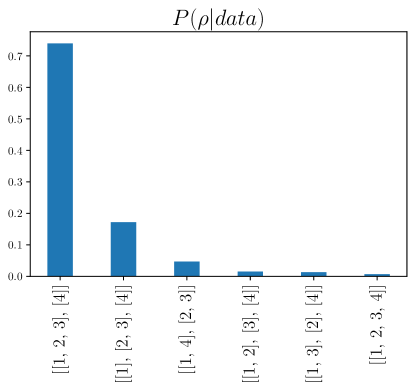
Figure 5: Posterior probability of $\rho$ for Scenario IV.

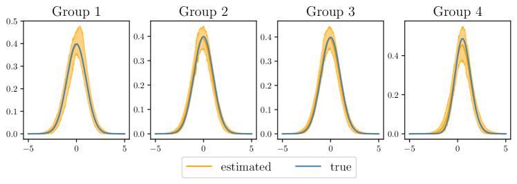
Figure 6: Density estimates and pointwise 95% posterior credible intervals for Scenario IV.

Finally, we test how our algorithm performs when the number of populations increases significantly. We do so by generating $100$ populations in Scenario VII as follows:

$$y_{ij} \stackrel{{\scriptstyle\mbox{\scriptsize iid}}}{{\sim}}0.5\mathcal{N}(-5,1)+0.5\mathcal{N}(5,1)\quad i=1,\ldots,20$$

$$y_{ij} \stackrel{{\scriptstyle\mbox{\scriptsize iid}}}{{\sim}}0.5\mathcal{N}(-5,1)+0.5\mathcal{N}(0,1)\quad i=21,\ldots,40$$

$$y_{ij} \stackrel{{\scriptstyle\mbox{\scriptsize iid}}}{{\sim}}0.5\mathcal{N}(0,1)+0.5\mathcal{N}(5,0.1)\quad i=41,\ldots,60$$

$$y_{ij} \stackrel{{\scriptstyle\mbox{\scriptsize iid}}}{{\sim}}0.5\mathcal{N}(-10,1)+0.5\mathcal{N}(0,1)\quad i=61,\ldots,80$$

$$y_{ij} \stackrel{{\scriptstyle\mbox{\scriptsize iid}}}{{\sim}}0.1\mathcal{N}(-10,1)+0.9\mathcal{N}(0,1)\quad i=81,\ldots,100.$$

Thus, full exchangeability holds within populations $\{1,\ldots,20\}$, $\{21,\ldots,40\}$, $\{41,\ldots,60\}$, $\{61,\ldots,80\}$ and $\{81,\ldots,100\}$ but not between these five groups. For each population $i$, $100$ datapoints were sampled independently.

To compute posterior inference, we run the Metropolised sampler with proposal (21). To get a rough idea of the computational costs associated to this large simulated dataset, we report that running the full Gibbs sampler would have required more than 24 hours on a 32-core machine (having parallelized all the computations which can be safely parallelized), while the Metropolised sampler ran in less than 3 hours on a 6-core laptop.

As a summary of the posterior distribution of the random partition $\mbox{\boldmath{$\rho$}}_{100}$, we compute the posterior similarity matrix $[P(c_{i}=c_{j}\,|\,data)]_{i,j=1}^{I}$. Estimates of these probabilities are straightforward to obtain using the output of the MCMC algorithm. Figure 7 shows the posterior similarity matrix as well as the density estimates of five different populations. It is clear that the clustering structure of the populations is recovered perfectly and that the density estimates are coherent with the true ones.

Figure 7: Density estimates (orange line), pointwise 95% posterior credible intervals (orange bands), true data generating densities (blue line) for groups 10, 30, 50, 70 and 90 and posterior similarity matrix (bottom right, white corresponds to 0.0 and dark blue to 1.0) in Scenario VII.

5.3 A note on the mixing

One aspect of the inference presented so far that is clear from all the simulated scenarios, is that the posterior simulation of $c$, and hence of the partition $\rho$, usually stabilizes around one particular value and then very rarely moves. This could be interpreted as a mixing issue of the MCMC chain. However, notice that once the “true” partition of the population is identified, it is extremely unlikely to move from that state, which can be seen directly from Equation (19). Indeed, moving from one state to another modifies the likelihood of an entire population. In particular, moving from a state where $c_{i}=c_{j}$ for two populations $i$ and $j$ that are actually homogeneous, to a state where $c_{i}\neq c_{j}$ is an extremely unlikely move.

To further illustrate the point, consider for ease of explanation the case of Simulation Scenario I where both populations are the same, and suppose that at a certain MCMC iteration we impute $c_{1}=c_{2}=1$. In order for the chain to jump to $c_{2}=2$, the “empty” mixing distribution $F_{2}$ must be sampled in such a way to give a reasonably high likelihood to all the data from the second population $y_{21},\ldots y_{2N_{2}}$; again, see (19). If one did not make use of pseudopriors, this would mean that $F_{2}$ would be sampled from the prior, thus making this transition virtually impossible. But even using pseudopriors, the transition remains quite unlikely. Indeed, once $c_{1}=c_{2}=1$, we get an estimate of $F_{1}$ using data from the two homogeneous groups, hence getting a much better estimate that one would get when $c_{1}\neq c_{2}$.

Nevertheless, in all simulation scenarios we tried this problem has not prevented the posterior simulation algorithm from identifying the correct partition of populations, as defined in these scenarios. In particular, we found that $P(\mbox{\boldmath{$\rho$}}_{4}^{true}|data)=0.75$ only in scenario IV , while in all the other cases we tried, the values of $P(\mbox{\boldmath{$\rho$}}_{4}^{true}|data)$ was greater than 0.9. We also computed the cluster estimate of the posterior of $\rho$ that minimizes the posterior expectation of Binder’s loss (Binder, 1978) under equal misclassification costs and of the variation of information loss (Wade and Ghahramani, 2018). In all the examples proposed, the “true” partition was correctly detected by both estimates.

6 Chilean grades dataset

The School of Mathematics at Pontificia Universidad Católica de Chile teaches many undergraduate courses to students from virtually all fields. When the number of students exceeds a certain maximum pre-established quota, several sections are formed, and courses are taught in parallel. There is a high degree of preparation in such cases, so as to guarantee that courses cover the same material and are coordinated to function as virtual copies of each other. In such cases, only the instructor changes across sections, but all materials related to the courses are the same, including exams, homework, assignments, projects, etc., and there is a shared team of graders that are common to all the parallel sections. According to the rules, every student gets a final grade on a scale from 1.0 to 7.0, using one decimal place, where 4.0 is the minimum passing grade. We consider here the specific case of a version of Calculus II, taught in parallel to three different sections (A, B and C) in a recent semester. Our main goal here is to examine the instructor effectiveness, by comparing the distributions of the final grades obtained by each of the three populations (sections). The sample sizes of these populations are 76, 65 and 50 respectively.

A possible way to model these data could be to employ a truncated normal distribution as the kernel in (2). However since our primary interest is to investigate the homogeneity of the underlying distributions and not to perform density estimates, we decided to first add a small amount of zero-mean Gaussian noise, with variance $0.1$ to the data (i.e. “jittering”) and then proceeded to standardize the whole dataset, by letting $y_{ij}^{new}=(y_{ij}-\bar{y})/s_{y}$, where $\bar{y}=(\sum_{ij}y_{ij})/(\sum_{i}N_{i})$ and $s^{2}_{y}=(\sum_{ij}(y_{ij}-\bar{y})^{2})/(\sum_{i}N_{i}-1)$ are the global sample mean and variance, respectively. In the sequel, index $i=1,2,3$ denotes sections A, B and C, respectively, as described above.

Figure 8 reports density estimates in all groups (i.e. posterior density means evaluated on a fixed grid of points and pointwise $95\%$ posterior credible intervals at each point $x$ in the grid), as well as the posterior distribution of the random partition $\rho$, obtained from the posterior distribution of $c$, getting rid of the label switching in a post-processing step (see also Section 5.2). From Figure 8 we see that the posterior distribution of $\rho$ gives high probability to the case of the three groups being all different as well as to the case when the first and third groups are homogeneous but different from the second one. This is in accordance with a visual analysis of the observed and estimated densities.

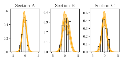
Figure 8: Density estimates and pointwise 95% posterior credible intervals for the three groups (left); posterior distribution of the clusters (right).

We considered several functionals of the random population distribution $F_{c_{i}}$ (see (3)) for $i=1,2,3$. Recall that, according to notation in (1), $F_{c_{i}}=G_{i}$. First of all, we consider the mean and variance functionals of the random density $p_{i}(y)=\int_{\Theta}k(y|\theta)F_{c_{i}}(d\theta)=\int_{\Theta}k(y|\theta)G_{i}(d\theta)$, for each $i=1,2,3$. Observe how they are functionals of the random probability $F_{c_{i}}=G_{i}$. Moreover, since Figure 8 seems to suggest that the three groups differ mainly due to their different asymmetries, we considered two more functionals of $G_{i}$, i.e. two indicators of skewness: Pearson’s moment coefficient of skewness sk and the measure of skewness with respect to the mode $\gamma_{M}$ proposed by Arnold and Groeneveld (1995). Pearson’s moment coefficient of skewness of the random variable $T$ is defined as $\text{sk}=\mathbb{E}[((T-\mathbb{E}(T))/\sqrt{\mathrm{Var}(T)})^{3}]$, while the measure of skewness with respect to the mode as $\gamma_{M}=1-2F_{T}(M_{T})$, where $M_{T}$ is the mode of $T$ and $F_{T}$ denotes its distribution function. The last functional of $G_{i}$ we consider is the probability, under the density $p_{i}(y)=\int_{\Theta}k(y|\theta)G_{i}(d\theta)$ of getting a passing grade ($\geq 4.0$ before normalization), that is

$$P_{4i}=\int_{(4-\bar{y})/s_{y}}^{+\infty}p_{i}(y)dy.$$

Table 3 shows the posterior mean of the functionals $\mu_{i}$, $\sigma_{i}^{2}$ (mean and variance functionals), $sk_{i}$, $\gamma_{Mi}$ and $P_{4i}$ of $p_{i}$, for $i=1,2,3$.

Section	${\mu_{i}}$	$\sigma_{i}^{2}$	${\text{sk}_{i}}$	${\gamma_{Mi}}$	${P_{4i}}$
A	-0.264	0.671	120.84	-0.01	0.53
B	0.438	1.428	-64.86	0.292	0.71
C	-0.171	0.943	55.60	-0.01	0.56

Table 3: Posterior means of functionals $\mu_{i},\ldots,P_{4i}$ of the population density $p_{i}$ for each Section A ($i=1$), B ($i=2$) and C ($i=3$) in the Chilean grades dataset. All the functionals refer to standardized data $\{y_{ij}^{new}=(y_{ij}-\bar{y})/s_{y}\}$.

To be clear, the posterior mean of the mean functional $\mu_{1}$ is computed as

$$\frac{1}{M}\sum_{\ell=1}^{M}\mu_{1}^{(\ell)}=\frac{1}{M}\sum_{\ell=1}^{M}\mathbb{E}[y\,|\,G_{1}^{(\ell)}]=\frac{1}{M}\sum_{\ell=1}^{M}\left(\int_{\mathbb{R}}yp_{1}^{(\ell)}(y)dy\right),$$

where $M$ is the MCMC sample size, and the superscript $(\ell)$ attached to a random variable denotes its value at the $\ell$–th MCMC iteration.

In agreement with the posterior distribution of the partition $\rho$, for all the functionals considered we observed close values for sections A and C, while both differ significantly from the values for section B. In summary, we conclude that section B presents a heavier right tail than sections A and C, hence it is characterized by a higher mean (positive) and also more spread across the range. Section B shows a larger (estimated) value for $P_{4}$, i.e. students in section B are more likely to pass the exam than their colleagues from the other sections. This seems to suggest that a higher concentration of good students (with high grades) was present in Section B, compared to A and C, possibly combined with a higher effectiveness of the instructor in this Section.

Figure 9: Posterior means of $(p_{i},p_{\ell})$, $i\neq\ell$, $i,\ell=A,B,C$, evaluated on a fixed grid in ${\mathbb{R}}^{2}$ for the Chilean grades dataset.

We also computed the pairwise $L^{1}$ distances between the estimated densities in the populations. If $\tilde{p}_{i}$ denotes the estimated density (posterior mean of $p_{i}$ evaluated in a grid of points) for each population, we found $d(\tilde{p}_{A},\tilde{p}_{B})=0.56$, $d(\tilde{p}_{A},\tilde{p}_{C})=0.15$ and $d(\tilde{p}_{B},\tilde{p}_{C})=0.44$. This confirms once again that the estimated densities for section A and C are closer than when comparing sections A and B and sections B and C.

To end the analysis, we show in Figure 9 estimated couples of densities $(p_{i},p_{\ell})$, $i\neq\ell$, $i,\ell=1,2,3$, i.e. the posterior mean of $(p_{i},p_{\ell})$, evaluated on a fixed grid in ${\mathbb{R}}^{2}$. While sections A and C look independent (central panel in Figure 9), the (posterior) propensity of section B to get higher grades is confirmed in the left and right panels in Figure 9.

7 Discussion

Motivated by the traditional problem of testing homogeneity across $I$ different groups or populations, we have presented a model that is able to not only address the problem but also to perform a cluster analysis of the groups. The model is built on a prior for the population distributions that we termed the semi-hierarchical Dirichlet process, and it was shown to have good properties and also to perform well in synthetic and real data examples, also in case of $I=100$ groups. One of the driving features of our proposal was to solve the degeneracy limitation of nested constructions that has been pointed out by Camerlenghi et al. (2019a). The crucial aspect of the semi-HDP that solves this problem was described using the metaphor of a food court of Chinese restaurants with common and private dining area. The hierarchical construction introduces a random partition at the population level, which allows for identifying possible clusters of internally homogeneous groups.

Our examples focus on unidimensional data, though extensions to multivariate responses can be straightforwardly accommodated in our framework. However, scaling with respect to data dimension is not a property we claim to have. In fact, this is a situation shared with any type of hierarchical mixture models.

We studied support properties of the semi-HDP and also the posterior asymptotic behavior of the Bayes factor for the homogeneity test when $I=2$, as posed within the proposed hierarchical construction. We showed that the Bayes factor has the appropriate asymptotic behavior under the alternative hypothesis of partial exchangeability, but a final answer under the assumption of truly exchangeable data is still pending. The lack of asymptotic guarantees is not at all specific to our case. In fact, this situation is rather common to all model selection problems when the hypothesis are not well separated and at least one of the two models under comparison is “truly” nonparametric, as, for instance, in Bhattacharya and Dunson (2012) and Tokdar and Martin (2019). Indeed, as discussed in Tokdar and Martin (2019), it is not even clear if in such cases the need for an upper bound on the prior mass under the more complex model is a natural requirement or rather a technical one. More generally, intuition about BFs (at least in parametric cases) is that they tend to favor the more parsimonious model. In the particular context described in Section 3.3, model $M_{1}$ can be regarded as a degenerate case of model $M_{2}$, even though they are “equally complicated”. In this case, the above intuition evaporates, since technically, embedding one model in the other is still one infinite-dimensional model contained in another infinite-dimensional model, and it is probably meaningless to ask which model is “simpler”. Under this scenario exploratory use of discrepancy measures, such as those discussed in Gelman et al. (1996), may offer some guidance.

In the simulation studies presented, our model always recovers the true latent clustering among groups, thus providing empirical evidence in favor of our model to perform homogeneity tests. We provide some practical suggestions when the actual interest is on making this decision. Our insight is that in order to prove asymptotic consistency of the Bayes factor, one should introduce explicit separation between the competing hypotheses. One possible way to accomplish this goal is, for example, by introducing some kind of repulsion among the mixing measures $F_{i}$’s in the model. This point will be focus of further study.

Appendix A Proofs

Proof of Proposition 3.1.
Consider $I=2$ for ease of exposition. We aim at showing that under suitable choices of $G_{0}$ and $G_{00}$, the vector of random probability measures $(G_{1},G_{2})$, where $G_{i}=F_{c_{i}}$ has full support on $\mathbb{P}_{\Theta}\times\mathbb{P}_{\Theta}$.

This means that for every couple of distributions $(g_{1},g_{2})\in\mathbb{P}_{\Theta}\times\mathbb{P}_{\Theta}$, every weak neighborhood $W_{1}\times W_{2}$ of $(g_{1},g_{2})$ receives non null probability. In short, this condition entails $\pi_{\mbox{\boldmath{$G$}}}(W_{1}\times W_{2})>0$. Since $G_{i}=F_{c_{i}}$, we have that

$$\pi_{\mbox{\boldmath{$G$}}}(W_{1}\times W_{2})=\sum_{l,m=1}^{2}\pi_{F_{l},F_{m}}(W_{1}\times W_{2})\pi_{c}(l,m)>\pi_{F_{1},F_{2}}(W_{1}\times W_{2})\pi_{c}(1,2).$$

Hence, since we are assuming that $\pi_{c}(l,m)>0$ for all $l,m$, it is sufficient to show that $\pi_{F_{1},F_{2}}$, that is the measure associated to the SemiHDP prior with $I=2$, has full weak support.

In the following, with a slight abuse of notation we denote by $\pi_{F_{1},F_{2}\,|\,\widetilde{G}}(W_{1}\times W_{2})$ the measure associated to the SemiHDP prior, conditional to a particular value of $\widetilde{G}$. We distinguish three cases: $\kappa=1$, $0<\kappa<1$ and $\kappa=0$. The case $\kappa=1$ is trivial, since $F_{1}$ and $F_{2}$ are marginally independently distributed with Dirichlet process prior, so that $\pi_{F_{1},F_{2}}(W_{1}\times W_{2})=\mathcal{D}_{\alpha G_{0}}(W_{1})\mathcal{D}_{\alpha G_{0}}(W_{2})>0$ as long as $G_{0}$ has full support in $\Theta$ (see, for example, Ghosal and Van der Vaart, 2017).

Secondly consider $0<\kappa<1$, we show that as long as $G_{0}$ has full support, then also $\pi_{\mbox{\boldmath{$G$}}}$ will have full support, regardless of the properties of $G_{00}$. We have

$$\pi_{F_{1},F_{2}}(W_{1}\times W_{2})=\int_{\mathbb{P}_{\Theta}}\pi_{F_{1},F_{2}\,|\,\widetilde{G}}(W_{1}\times W_{2})\mathcal{L}(d\widetilde{G})=\int_{\mathbb{P}_{\Theta}}\mathcal{D}_{\alpha\widetilde{P}}(W_{1})\mathcal{D}_{\alpha\widetilde{P}}(W_{2})\mathcal{L}(d\widetilde{G}).$$ (24)

Now observe that if $G_{0}$ has full support, also $\widetilde{P}=\kappa G_{0}+(1-\kappa)\widetilde{G}$ will have full support, for any value of $\widetilde{G}$. Hence by the properties of the Dirichlet Process, we get that $\pi_{F_{1},F_{2}}(W_{1}\times W_{2})>0$ since the integrand in (24) is bounded away from zero.

The case $\kappa=0$ is more delicate and requires additional work. We follow the path outlined in De Blasi et al. (2013), extending it to our hierarchical case. In the following, let $\mathbb{S}^{m}$ denote the $m-1$ dimensional simplex, i.e.

$$\mathbb{S}^{m}:=\{(z_{1},\ldots,z_{m})\in\mathbb{R}^{m}\ :\ 0\leq z_{h}\leq 1,\ h=1,\ldots,m,\ \sum_{h=1}^{m}z_{h}=1\}$$

Let $d_{w}$ denote the Prokhorov metric on $\mathbb{P}_{\Theta}$, which, as it is well known, metrizes the topology of the weak convergence on $\mathbb{P}_{\Theta}$. Moreover, being $\Theta$ separable, $(\mathbb{P}_{\Theta},d_{w})$ is separable as well and the set of discrete measures with a finite number of point masses is dense in $\mathbb{P}_{\Theta}$.

Hence, for any $(g_{1},g_{2})$ and any $\epsilon>0$, there exist two discrete measures with weights $\mbox{\boldmath{$p$}}^{(i)}\in\mathbb{S}^{k_{i}}$ and points $\mbox{\boldmath{$x$}}^{(i)}\in\Theta^{k_{i}}$ for $i=1,2$ such that $d_{w}(F_{\mbox{\boldmath{$p$}}^{(i)},\mbox{\boldmath{$x$}}^{(i)}},g_{i})<\epsilon$, where $F_{\mbox{\boldmath{$p$}}^{(i)},\mbox{\boldmath{$x$}}^{(i)}}=\sum_{k}p^{(i)}_{k}\delta_{x^{(i)}_{k}}$. The difficulty when $\kappa=0$ is that conditionally on $\widetilde{G}$, the measure $\mathcal{D}_{\alpha\widetilde{G}}$ does not have full weak support. Indeed, its support is concentrated on the measures that have the same atoms of $\widetilde{G}$. The proof will proceed as follows: start by defining weak neighborhoods $W_{i}$ of $F_{\mbox{\boldmath{$p$}}^{(i)},\mbox{\boldmath{$x$}}^{(i)}}$ by looking at neighborhoods of their weights $\mbox{\boldmath{$p$}}^{(i)}$ ($U_{i}$) and atoms $\mbox{\boldmath{$x$}}^{(i)}$ ($V_{i}$). Secondly, we join these neighborhoods. If $\widetilde{G}(\omega)$ belongs to this union (and this occurs with positive probability), we guarantee that the atoms of both of $F_{1}$ and $F_{2}$, that are shared with $\widetilde{G}$, are suited to approximate both $F_{\mbox{\boldmath{$p$}}^{(i)},\mbox{\boldmath{$x$}}^{(i)}}$, $i=1,2$. Hence, by the properties of the Dirichlet Process one gets the support property.

More in detail, define the sets

$$V_{i}(\delta)=\{\mbox{\boldmath{$x$}}_{i}\in\Theta^{k_{i}}\ s.t.\ |x_{ij}-x^{(i)}_{j}|<\delta\},i=1,2$$

and let $V=V_{1}\cup V_{2}$. Then we operate a change of index by concatenating $\mbox{\boldmath{$x$}}^{(1)}$ and $\mbox{\boldmath{$x$}}^{(2)}$, and call it $\mbox{\boldmath{$x$}}^{*}$, i.e. $\mbox{\boldmath{$x$}}^{*}=[\mbox{\boldmath{$x$}}^{(1)},\mbox{\boldmath{$x$}}^{(2)}]$. Hence we characterize the set $V$ as

$$V(\delta)=\{\mbox{\boldmath{$x$}}\in\Theta^{k_{1}+k_{2}}\ s.t\ |x_{j}-x^{*}_{j}|<\delta\}.$$

Secondly, define $\mbox{\boldmath{$p$}}^{*}$ by concatenating $\mbox{\boldmath{$p$}}^{(1)}$ and and $\mbox{\boldmath{$p$}}^{(2)}$: $\mbox{\boldmath{$p$}}^{*}=[\mbox{\boldmath{$p$}}^{(1)},\mbox{\boldmath{$p$}}^{(2)}]$ and let

$$U_{1}(\eta) =\{\mbox{\boldmath{$p$}}\in\mathbb{S}^{k_{1}+k_{2}}\ s.t.\ |p_{j}-p^{*}_{j}|<\eta\text{ for }j=1,\ldots,k_{1},\ |p_{j}-0|<\eta\text{ elsewhere}\}$$

$$U_{2}(\eta) =\{\mbox{\boldmath{$p$}}\in\mathbb{S}^{k_{1}+k_{2}}\ s.t.\ |p_{j}-p^{*}_{j}|<\eta\text{ for }j=k_{1}+1,\ldots,k_{1}+k_{2},\ |p_{j}-0|<\eta\text{ elsewhere}\}$$

Finally, define the following neighborhoods

$$W_{i} :=\{\sum_{j=1}^{k_{1}+k_{2}}p_{j}\delta_{x_{j}}\text{ for any }\mbox{\boldmath{$p$}}\in U_{i},\text{ and any }\mbox{\boldmath{$x$}}\in V\},i=1,2$$

$$W_{0} :=\{\sum_{j=1}^{k_{1}+k_{2}}p_{j}\delta_{x_{j}}\text{ for any }\mbox{\boldmath{$p$}}\in\mathbb{S}^{k_{1}+k_{2}},\text{ and any }\mbox{\boldmath{$x$}}\in V\}.$$

This means that the $V_{i}$ sets are the neighborhoods of the atoms $\mbox{\boldmath{$x$}}_{i}$ that are well suited to approximate $F_{\mbox{\boldmath{$p$}}^{(i)},\mbox{\boldmath{$x$}}^{(i)}}$ and $V$ is their union. The sets $U_{i}$, $i=1,2$, instead, are related to the weights of $F_{\mbox{\boldmath{$p$}}^{(i)},\mbox{\boldmath{$x$}}^{(i)}}$. In particular, each $U_{i}$ is constructed in such a way to approximate well $\mbox{\boldmath{$p$}}^{(i)}$ (a vector in $\mathbb{S}^{k_{i}}$) with a vector of weights in $\mathbb{S}^{k_{1}+k_{2}}$. This is necessary because if $\widetilde{G}$ has support points in $V$, so will do the draws $F_{1}$ and $F_{2}$ from $\mathcal{D}_{\alpha\widetilde{G}}$. However, by assigning a negligible weight in $U_{1}$ to the atoms $\mbox{\boldmath{$x$}}^{(2)}$ and vice-versa for the atoms $\mbox{\boldmath{$x$}}^{(1)}$ in $U_{2}$, we guarantee that the probability measures in $W_{i}$ constitute a weak neighborhood of $F_{\mbox{\boldmath{$p$}}^{(i)},\mbox{\boldmath{$x$}}^{(i)}}$ for each $i=1,2$.

From De Blasi et al. (2013), it is sufficient to show that $\pi_{F_{1},F_{2}}(W_{1}\times W_{2})>0$ since for appropriate choices of $\eta$ and $\delta$ one has that $d_{w}(\widetilde{F}_{1},g_{1})+d_{w}(\widetilde{F}_{2},g_{2})<\epsilon$ for all choices of $\widetilde{F}_{1}\in W_{1}$ and $\widetilde{F}_{2}\in W_{2}$. Hence

$$\pi_{F_{1},F_{2}}(W_{1}\times W_{2})=\int_{\mathbb{P}_{\Theta}}\pi_{F_{1},F_{2}\,|\,\widetilde{G}}(W_{1}\times W_{2})\mathcal{L}(d\widetilde{G}) \geq\int_{W_{0}}\pi_{F_{1},F_{2}\,|\,\widetilde{G}}(W_{1},W_{2})\mathcal{L}(d\widetilde{G})$$

$$=\int_{W_{0}}\mathcal{D}_{\alpha\widetilde{G}}(W_{1})\mathcal{D}_{\alpha\widetilde{G}}(W_{2})\mathcal{L}(d\widetilde{G})$$

Now observe that for any $\widetilde{G}\in W_{0}$, we have that $\mathcal{D}_{\alpha\widetilde{G}}(W_{i})>0$. This follows again from the properties of the Dirichlet process, since for any value of $\widetilde{G}(\omega)$, there exists a non-empty set $\widetilde{W}_{i}\subset W_{i}$, $\widetilde{W}_{i}=\{\widetilde{F}_{i}\in W_{i}:\ supp(\widetilde{F}_{i})\subset supp(\widetilde{G})\}$. Hence $\pi_{F_{1},F_{2}\,|\,\widetilde{G}}(W_{1}\times W_{2})\geq\pi_{F_{1},F_{2}\,|\,\widetilde{G}}(\widetilde{W}_{1}\times\widetilde{W}_{2})>0$, since the Dirichlet process gives positive probability to the weak neighborhoods of measures whose support is contained in the support of its base measure, i.e. $\widetilde{G}$. $\Box$

Proof of Covariance of the semi-HDP.
If $(F_{1},F_{2})\sim semiHDP(\alpha,\gamma,\kappa,G_{0},G_{0})$, then

$$\text{cov}(F_{1}(A)F_{2}(B)) =\mathbb{E}\left[F_{1}(A)F_{2}(B)\right]-\mathbb{E}\left[F_{1}(A)\right]\mathbb{E}\left[F_{2}(B)\right]$$

$$=\mathbb{E}\left[\mathbb{E}\left[F_{1}(A)F_{2}(B)\,|\,\widetilde{P}\right]\right]-\mathbb{E}\left[\mathbb{E}\left[F_{1}(A)\,|\,\widetilde{P}\right]\right]\mathbb{E}\left[\mathbb{E}\left[F_{2}(B)\,|\,\widetilde{P}\right]\right]$$

$$=\mathbb{E}\left[\mathbb{E}\left[F_{1}(A)\,|\,\widetilde{P}\right]\mathbb{E}\left[F_{2}(B)\,|\,\widetilde{P}\right]\right]-G_{0}(A)G_{0}(B)$$

$$=\mathbb{E}\left[\widetilde{P}(A)\widetilde{P}(B)\right]-G_{0}(A)G_{0}(B)$$

$$=\kappa^{2}G_{0}(A)G_{0}(B)+\kappa(1-\kappa)G_{0}(A)\mathbb{E}\left[\widetilde{G}(B)\right]+\kappa(1-\kappa)G_{0}(B)\mathbb{E}\left[\widetilde{G}(A)\right]$$

$$\quad+(1-\kappa)^{2}\mathbb{E}\left[\widetilde{G}(A)\widetilde{G}(B)\right]-G_{0}(A)G_{0}(B)$$

$$=(1-\kappa)^{2}\mathbb{E}\left[\widetilde{G}(A)\widetilde{G}(B)\right]-(1-\kappa)^{2}G_{0}(A)G_{0}(B)$$

$$=(1-\kappa)^{2}\text{cov}(\widetilde{G}(A),\widetilde{G}(B))=\frac{(1-\kappa)^{2}}{1+\gamma}\left(G_{0}(A\cap B)-G_{0}(A)G_{0}(B)\right).$$

The last equality follows because $\widetilde{G}$ is a Dirichlet process. $\Box$

Higher order moments.
To compute higher order moments, we make use of a result from Argiento et al. (2019). Let $F_{1}\,|\,\widetilde{P}\sim\mathcal{D}_{\alpha\widetilde{P}}$ as in (5) - (7); then one has, for any set $A\in\mathcal{B}(\Theta)$:

$$\mathbb{E}[F_{1}(A)^{n}\,|\,\widetilde{G}]=\sum_{t=1}^{n}\widetilde{P}(A)^{t}P(K_{n}=t),$$

where $K_{n}$ is the random variable representing the number of clusters in a sample of size $n$; see (15) in Argiento et al. (2019). If, as in our case, the base measure is not absolutely continuous, the term clusters might be misleading as they do not coincide with the unique values in the sample, but rather with the number of the tables in the Chinese restaurant process. In the following we refer to cluster or table interchangeably. Hence, we have:

$$\mathbb{E}[F_{1}(A)^{n}] =\mathbb{E}[\mathbb{E}[F_{1}(A)^{n}\,|\,\widetilde{G}]]=\mathbb{E}\left[\sum_{t=1}^{n}\widetilde{P}(A)^{t}P(K_{n}=t)\right]$$

$$=\mathbb{E}\left[\sum_{t=1}^{n}P(K_{n}=t)\sum_{h=0}^{t}\binom{t}{h}(\kappa G_{0}(A))^{t-h}\times((1-\kappa)\widetilde{G}(A))^{h}\right]$$

$$=\sum_{t=1}^{n}P(K_{n}=t)\sum_{h=0}^{t}\binom{t}{h}(\kappa G_{0}(A))^{t-h}(1-\kappa)^{h}\mathbb{E}[\widetilde{G}(A)^{h}]$$

$$=\sum_{t=1}^{n}P(K_{n}=t)\sum_{h=0}^{t}\binom{t}{h}(\kappa G_{0}(A))^{t-h}(1-\kappa)^{h}\sum_{m=1}^{h}G_{00}(A)P(\widetilde{K}_{h}=m),$$

where $\widetilde{K}_{h}$ is the number of clusters from a sample of size $h$ from the DP $\widetilde{G}$. Moreover, if we assume $G_{0}=G_{00}$ we get

$$\mathbb{E}[F_{1}(A)^{n}]=\sum_{t=1}^{n}P(K_{n}=t)\sum_{h=0}^{t}\binom{t}{h}\kappa^{t-h}(1-\kappa)^{h}\sum_{m=1}^{h}G_{0}(A)^{t-h+m}P(K_{h}=m).$$

Figure 10: 3-rd moment of $F_{1}(A)$ for increasing values of $\kappa$ and various values of $G_{0}(A)$.

Figure 10 shows the effect of the parameter $\kappa$ over $\mathbb{E}[F_{1}(A)^{3}]$ for various values of $G_{0}(A)$. The limiting cases of the standard Dirichlet process and the Hierarchical Dirichlet Process are recovered when $\kappa=1$ and $\kappa=0$ respectively.

Proof of Proposition 3.2.
Indicating with $\tau_{j}$ the shared unique values between $\mbox{\boldmath{$\theta$}}_{1}$ and $\mbox{\boldmath{$\theta$}}_{2}$, and with $\theta^{*}_{ij}$ the unique values in sample $\mbox{\boldmath{$\theta$}}_{i}$ that are specific to group $i$, i.e. not shared, the pEPPF, given $c$, can be written as:

$$\Pi^{(N)}_{k}(\mbox{\boldmath{$n$}}_{1},\mbox{\boldmath{$n$}}_{2},\mbox{\boldmath{$q$}}_{1},\mbox{\boldmath{$q$}}_{2}|\mbox{\boldmath{$c$}})=\int_{\Theta^{k}}\mathbb{E}\left[\prod_{j=1}^{k_{1}}F_{c_{1}}^{n_{1j}}(d\theta^{*}_{1j})\prod_{j=1}^{k_{2}}F_{c_{2}}^{n_{2j}}(d\theta^{*}_{2j})\prod_{j=1}^{k_{0}}F_{c_{1}}^{q_{1j}}(d\tau_{j})F_{c_{2}}^{q_{2j}}(d\tau_{j})\right].$$

See (23) in Camerlenghi et al. (2019a). Marginalizing out $c$ we obtain that:

$$\Pi^{(N)}_{k}(\mbox{\boldmath{$n$}}_{1},\mbox{\boldmath{$n$}}_{2},\mbox{\boldmath{$q$}}_{1},\mbox{\boldmath{$q$}}_{2})=\sum_{l,m=1}^{2}\pi_{\mbox{\boldmath{$c$}}}(\mbox{\boldmath{$c$}}=(l,m))\Pi^{(N)}_{k}(\mbox{\boldmath{$n$}}_{1},\mbox{\boldmath{$n$}}_{2},\mbox{\boldmath{$q$}}_{1},\mbox{\boldmath{$q$}}_{2}|\mbox{\boldmath{$c$}}=(l,m)).$$

The cases $\mbox{\boldmath{$c$}}=(1,1)$ and $\mbox{\boldmath{$c$}}=(2,2)$ can be easily managed as it corresponds to full exchangeability and the EPPF corresponding to those cases is already available. Hence, let us consider the case when $\mbox{\boldmath{$c$}}=(1,2)$, as the case $\mbox{\boldmath{$c$}}=(2,1)$ will be identical because the $F_{i}$’s are iid.

$$\Pi^{(N)}_{k} (\mbox{\boldmath{$n$}}_{1},\mbox{\boldmath{$n$}}_{2},\mbox{\boldmath{$q$}}_{1},\mbox{\boldmath{$q$}}_{2}|\mbox{\boldmath{$c$}}=(1,2))=\int_{\Theta^{k}}\mathbb{E}\left[\prod_{j=1}^{k_{1}}F_{1}^{n_{1j}}(d\theta^{*}_{1j})\prod_{j=1}^{k_{2}}F_{2}^{n_{2j}}(d\theta^{*}_{2j})\prod_{j=1}^{k_{0}}F_{1}^{q_{1j}}(d\tau_{j})F_{2}^{q_{2j}}(d\tau_{j})\right]$$

$$=\int_{\Theta^{k}}\mathbb{E}\left[\prod_{j=1}^{k_{1}}F_{1}^{n_{1j}}(d\theta^{*}_{1j})\prod_{j=1}^{k_{0}}F_{1}^{q_{1j}}(d\tau_{j})\right]\mathbb{E}\left[\prod_{j=1}^{k_{2}}F_{2}^{n_{2j}}(d\theta^{*}_{2j})\prod_{j=1}^{k_{0}}(d\tau_{j})F_{2}^{q_{2j}}(d\tau_{j})\right]$$

since $F_{1}$ and $F_{2}$ are independent. The first expected value is the joint probability of $\Pi_{k_{1}+k_{0}}^{N_{1}}$ (the EPPF of a partition of $N_{1}$ objects into $k_{1}+k_{0}$ groups with vectors of frequencies $\mbox{\boldmath{$n$}}_{1},\mbox{\boldmath{$q$}}_{1}$) and the set of unique values is denoted by $(x_{11},\dots,x_{1k_{1}},\tau_{1},\dots\tau_{k_{0}})$. Similarly for the second expected value. Because $F_{1}\sim\mathcal{D}_{\alpha G_{0}}$, we can rewrite the expected value as:

$$\mathbb{E}\left[\prod_{j=1}^{k_{1}}F_{1}^{n_{1j}}(d\theta^{*}_{1j})\prod_{j=1}^{k_{0}}F_{1}^{q_{1j}}(d\tau_{j})\right]$$

$$\quad=\frac{\alpha_{1}^{k_{1}+k_{0}}\Gamma(\alpha_{1})}{\Gamma(\alpha_{1}+N_{1})}\prod_{j=1}^{k_{1}}\Gamma(n_{1j})\prod_{j=1}^{k_{0}}\Gamma(q_{1j})\prod_{j=1}^{k_{1}}G_{0}(d\theta^{*}_{1j})\prod_{j=1}^{k_{0}}G_{0}(d\tau_{j}).$$

Hence, we have that

$$\Pi^{(N)}_{k} (\mbox{\boldmath{$n$}}_{1},\mbox{\boldmath{$n$}}_{2},\mbox{\boldmath{$q$}}_{1},\mbox{\boldmath{$q$}}_{2}|\mbox{\boldmath{$c$}}=(1,2))=$$

$$\quad=\int_{\Theta^{k}}\mathbb{E}\left[\prod_{j=1}^{k_{1}}F_{1}^{n_{1j}}(d\theta^{*}_{1j})\prod_{j=1}^{k_{0}}F_{1}^{q_{1j}}(d\tau_{j})\right]\mathbb{E}\left[\prod_{j=1}^{k_{2}}F_{2}^{n_{2j}}(d\theta^{*}_{2j})\prod_{j=1}^{k_{0}}(d\tau_{j})F_{2}^{q_{2j}}(d\tau_{j})\right]$$

$$\quad=\frac{\alpha_{1}^{k_{1}+k_{0}}\Gamma(\alpha_{1})}{\Gamma(\alpha_{1}+N_{1})}\frac{\alpha_{2}^{k_{2}+k_{0}}\Gamma(\alpha_{2})}{\Gamma(\alpha_{2}+N_{2})}\prod_{j=1}^{k_{1}}\Gamma(n_{1j})\prod_{j=1}^{k_{2}}\Gamma(n_{2j})\prod_{j=1}^{k_{0}}\Gamma(q_{1j})\Gamma(q_{2j})$$

$$\qquad\qquad\qquad\times\int_{\Theta^{k}}\prod_{j=1}^{k_{1}}G_{0}(d\theta^{*}_{1j})\prod_{j=1}^{k_{2}}G_{0}(d\theta^{*}_{2j})\prod_{j=1}^{k_{0}}G_{0}(d\tau_{j})G_{0}(d\tau_{j}).$$

Looking at the last integral, we can see that this is clearly 0 unless $k_{0}=0$, in fact, consider $k_{0}=1$:

$$\int_{\Theta^{k-1}}\prod_{j=1}^{k_{1}}G_{0}(d\theta^{*}_{1j})\prod_{j=1}^{k_{2}}G_{0}(d\theta^{*}_{2j})\int_{\Theta}G_{0}(dz)G_{0}(dz)$$

and observe that the last integral is integrating the product measure $G_{0}\times G_{0}$ on the straight line $y=x$, resulting thus in 0.

Summing up, if $k_{0}=0$ we get:

$$\Pi^{(N)}_{k}(\mbox{\boldmath{$n$}}_{1},\mbox{\boldmath{$n$}}_{2},\mbox{\boldmath{$q$}}_{1},\mbox{\boldmath{$q$}}_{2})= \pi_{1}\frac{\alpha^{k_{1}+k_{2}}\Gamma(\alpha)}{\Gamma(\alpha+N)}\prod_{j=1}^{k_{1}}\Gamma(n_{1j})\prod_{j=1}^{k_{2}}\Gamma(n_{2j})$$

$$+(1-\pi_{1})\frac{\alpha^{k_{1}+k_{2}}\Gamma(\alpha)^{2}}{\Gamma(\alpha+N_{1})\Gamma(\alpha+N_{2})}\prod_{j=1}^{k_{1}}\Gamma(n_{1j})\prod_{j=1}^{k_{2}}\Gamma(n_{2j})$$

else, if $k_{0}>0$:

$$\Pi^{(N)}_{k} (\mbox{\boldmath{$n$}}_{1},\mbox{\boldmath{$n$}}_{2},\mbox{\boldmath{$q$}}_{1},\mbox{\boldmath{$q$}}_{2})=$$

$$(1-\pi_{1})\frac{\alpha^{k_{1}+k_{2}+k_{0}}\Gamma(\alpha)}{\Gamma(\alpha+N)}\prod_{j=1}^{k_{1}}\Gamma(n_{1j})\prod_{j=1}^{k_{2}}\Gamma(n_{2j})\prod_{j=1}^{k_{0}}\Gamma(q_{1j}+q_{2j})$$

which can be rewritten down as in Camerlenghi et al. (2019a); call

$$\Phi_{k}^{(N)}(\mbox{\boldmath{$n$}}_{1},\mbox{\boldmath{$n$}}_{2},\mbox{\boldmath{$q$}}_{1}+\mbox{\boldmath{$q$}}_{2})=\frac{\alpha^{k_{1}+k_{2}+k_{0}}\Gamma(\alpha)}{\Gamma(\alpha+N)}\prod_{j=1}^{k_{1}}\Gamma(n_{1j})\prod_{j=1}^{k_{2}}\Gamma(n_{2j})\prod_{j=1}^{k_{0}}\Gamma(q_{1j}+q_{2j})$$

the EPPF of the fully exchangeable case, and

$$\Phi_{k_{0}+k_{i}}^{(N_{i})}(\mbox{\boldmath{$n$}}_{i},\mbox{\boldmath{$q$}}_{i})=\frac{\alpha^{k_{i}+k_{0}}\Gamma(\alpha)}{\Gamma(\alpha+N_{i})}\prod_{j=1}^{k_{i}}\Gamma(n_{ij})\prod_{j=1}^{k_{0}}\Gamma(q_{ij})$$

the marginal EPPF for the individual groups $i=1,2$. We have that:

$$\Pi^{(N)}_{k}(\mbox{\boldmath{$n$}}_{1},\mbox{\boldmath{$n$}}_{2},\mbox{\boldmath{$q$}}_{1},\mbox{\boldmath{$q$}}_{2})=\pi_{1}\Phi_{k}^{(N)}(\mbox{\boldmath{$n$}}_{1},\mbox{\boldmath{$n$}}_{2},\mbox{\boldmath{$q$}}_{1}+\mbox{\boldmath{$q$}}_{2})+(1-\pi_{1})\Phi_{k_{0}+k_{1}}^{(N_{1})}(\mbox{\boldmath{$n$}}_{1},\mbox{\boldmath{$q$}}_{1})\Phi_{k_{0}+k_{1}}^{(N_{2})}(\mbox{\boldmath{$n$}}_{2},\mbox{\boldmath{$q$}}_{2})I(k_{0}=0)$$

which is (13). $\Box$

Proof of Proposition 3.3.
Of course, the marginal law of $(\mbox{\boldmath{$\theta$}}_{1},\ldots,\mbox{\boldmath{$\theta$}}_{I})$, conditional to $c$, can be computed as

$$\mathcal{L} (d\mbox{\boldmath{$\theta$}}_{1},\ldots d\mbox{\boldmath{$\theta$}}_{I}\,|\,\mbox{\boldmath{$c$}})=\int_{\mathbb{P}_{\Theta}}\ldots\int_{\mathbb{P}_{\Theta}}\mathcal{L}(d\mbox{\boldmath{$\theta$}}_{1},\ldots d\mbox{\boldmath{$\theta$}}_{I}\,|\,F_{1},\ldots F_{I},\mbox{\boldmath{$c$}})\mathcal{L}(dF_{1},\ldots dF_{I}).$$

Now we operate a change of indices and call $\mbox{\boldmath{$\theta$}}_{r}=\{\mbox{\boldmath{$\theta$}}_{i}=(\theta_{i1},\ldots\theta_{iN_{i}}):c_{i}=r\}$, so that $(\mbox{\boldmath{$\theta$}}_{1},\ldots\mbox{\boldmath{$\theta$}}_{I})=(\mbox{\boldmath{$\theta$}}_{r_{1}},\ldots\mbox{\boldmath{$\theta$}}_{r_{R}})$ where $R$ is the number of unique values in $c$, i.e. the number of non-empty restaurants. We get

$$\mathcal{L}(d\mbox{\boldmath{$\theta$}}_{1},\ldots d\mbox{\boldmath{$\theta$}}_{I}\,|\,\mbox{\boldmath{$c$}}) =\int_{\mathbb{P}_{\Theta}}\int_{\mathbb{P}_{\Theta}}\ldots\int_{\mathbb{P}_{\Theta}}\mathcal{L}(d\mbox{\boldmath{$\theta$}}_{r_{1}},\ldots d\mbox{\boldmath{$\theta$}}_{r_{R}}\,|\,F_{1},\ldots F_{I},\mbox{\boldmath{$c$}})\mathcal{L}(dF_{1},\ldots dF_{I}\,|\,\widetilde{G})\mathcal{L}(d\widetilde{G})$$

$$=\int_{\mathbb{P}_{\Theta}}\left(\prod_{i=1}^{R}\int_{\mathbb{P}_{\Theta}}\mathcal{L}(d\mbox{\boldmath{$\theta$}}_{r_{i}}\,|\,F_{r_{i}})\mathcal{L}(dF_{r_{i}}\,|\,\widetilde{G})\right)\mathcal{L}(d\widetilde{G}).$$

Observe that

$$\int_{\mathbb{P}_{\Theta}}\mathcal{L}(d\mbox{\boldmath{$\theta$}}_{r_{i}}\,|\,F_{r_{i}})\mathcal{L}(dF_{r_{i}}\,|\,\widetilde{G})=\mathcal{L}(\rho_{r_{i}})\prod_{j=1}^{H_{r_{i}}}\widetilde{P}(d\theta^{*}_{r_{i}j}),$$

where $\rho_{r_{i}}$ is the partition induced by the $\ell$-clusters in the $r_{i}$ restaurant. We use the same definition of $\ell$-cluster as in Argiento et al. (2019). We underline that $\{\theta^{*}_{r_{i}j},j=1,\ldots,H_{r_{i}}\}$ are not the unique values in the sample, since the base measure is atomic. Hence we have

$$\int_{\mathbb{P}_{\Theta}}\left(\prod_{i=1}^{R}\int_{\mathbb{P}_{\Theta}}\mathcal{L}(d\mbox{\boldmath{$\theta$}}_{r_{i}}\,|\,F_{r_{i}})\mathcal{L}(dF_{r_{i}}\,|\,\widetilde{G})\right)\mathcal{L}(d\widetilde{G})$$

$$=\left(\prod_{i=1}^{R}\mathcal{L}(\rho_{r_{i}})\right)\int_{\mathbb{P}_{\Theta}}\prod_{i=1}^{R}\prod_{j=1}^{H_{r_{i}}}\widetilde{P}(d\theta^{*}_{r_{i}j})\mathcal{L}(d\widetilde{G}).$$

Now observe how the values $\{\theta^{*}_{rj}:\ r=1,\ldots R,j=1,\ldots H_{r_{i}}\}$ are all iid from $\widetilde{P}$. So, there is no need for the division into restaurants anymore. We can thus stack all the vectors $\mbox{\boldmath{$\theta$}}^{*}_{r_{i}}$ together, apply a change of indices $(r_{i},j)\rightarrow l$ so that now these $\{\theta^{*}_{r_{i}}\}$ are represented by $(\theta^{*}_{1},\ldots,\theta^{*}_{L})$ and

$$\mathcal{L}(d\mbox{\boldmath{$\theta$}}_{1},\ldots d\mbox{\boldmath{$\theta$}}_{I}\,|\,\mbox{\boldmath{$c$}}) =\prod_{i=1}^{R}\mathcal{L}(\rho_{r_{i}})\int_{\mathbb{P}_{\Theta}}\prod_{l=1}^{L}\widetilde{P}(d\theta^{*}_{l})\mathcal{L}(d\widetilde{G})$$

$$=\prod_{i=1}^{R}\mathcal{L}(\rho_{r_{i}})\int_{\mathbb{P}_{\Theta}}\prod_{l=1}^{L}\left(\kappa G_{0}(d\theta^{*}_{l})+(1-\kappa)\widetilde{G}(d\theta^{*}_{l})\right)\mathcal{L}(d\widetilde{G}).$$

Now, as done in Section 2.2, we introduce a set of latent variables $\mbox{\boldmath{$h$}}=(h_{1},\ldots,h_{L})$, $h_{l}\stackrel{{\scriptstyle\mbox{\scriptsize iid}}}{{\sim}}\text{Bernoulli}(\kappa)$, that gives

$$\mathcal{L} (d\mbox{\boldmath{$\theta$}}_{1},\ldots d\mbox{\boldmath{$\theta$}}_{I}\,|\,\mbox{\boldmath{$c$}})=\prod_{i=1}^{R}\mathcal{L}(\rho_{r_{i}})\sum_{\mbox{\boldmath{$h$}}\in\{0,1\}^{L}}p(\mbox{\boldmath{$h$}})\int_{P}\prod_{l=1}^{L}G_{0}(d\theta^{*}_{l})^{h_{l}}\times\widetilde{G}(d\theta^{*}_{l})^{1-h_{l}}\mathcal{L}(d\widetilde{G})$$

$$=\prod_{i=1}^{R}\mathcal{L}(\rho_{r_{i}})\sum_{\mbox{\boldmath{$h$}}\in\{0,1\}^{L}}p(\mbox{\boldmath{$h$}})\prod_{l=1}^{L}G_{0}(d\theta^{*}_{l})^{h_{l}}\int_{P}\prod_{l=1}^{L}\widetilde{G}(d\theta^{*}_{l})^{1-h_{l}}\mathcal{L}(d\widetilde{G})$$

$$=\prod_{i=1}^{R}\mathcal{L}(\rho_{r_{i}})\sum_{\mbox{\boldmath{$h$}}\in\{0,1\}^{L}}p(\mbox{\boldmath{$h$}})\prod_{l=1}^{L}G_{0}(d\theta^{*}_{l})^{h_{l}}\times\mathcal{L}(\eta\,|\,\mbox{\boldmath{$h$}})\prod_{k=1}^{M(\eta)}G_{00}(d\theta^{**}_{k}),$$

where $\eta$ is the partition of the $\{\theta^{*}_{l}:\ l=1,\ldots,L\text{ and }h_{l}=0\}$, i.e. the partition of $\sum_{l=1}^{L}(1-h_{l})$ objects arising form the Dirichlet process $\widetilde{G}$, while $\{\theta^{**}_{k}\}$ are the unique values among $\{\theta^{*}_{l}:\ l=1,\ldots,L\text{ and }h_{l}=0\}$ and $p(\mbox{\boldmath{$h$}})=\prod_{l=1}^{L}\kappa^{h_{l}}(1-\kappa)^{1-h_{l}}$ is the joint distribution of $h$. $\Box$

Proof of Proposition 3.4.
Model $M_{2}$ defines a prior $\Pi_{2}$ on the space of densities $(p,q)\in\mathbb{P}_{\mathbb{Y}}\times\mathbb{P}_{\mathbb{Y}}$. On the other hand, model $M_{1}$ defines a prior on $\mathbb{P}_{\mathbb{Y}}$. However, by embedding $\mathbb{P}_{\mathbb{Y}}$ in the product space $\mathbb{P}_{\mathbb{Y}}\times\mathbb{P}_{\mathbb{Y}}$ via the mapping $p\mapsto(p,p)$, we can also consider the prior $\Pi_{1}$ induced by model $M_{1}$ as a measure on (a subset of) $\mathbb{P}_{\mathbb{Y}}\times\mathbb{P}_{\mathbb{Y}}$.

Now, showing that $\Pi_{2}$ satisfies the Kullback-Leibler property is a straightforward application of Theorem 3 in Wu and Ghosal (2008), under the same set of assumptions on the kernel $k(\cdot|\theta)$, and on $p_{0}$ and $q_{0}$, that we do not report here. Notice that these assumptions are satisfied when $k(\cdot|\theta)$ is the univariate Gaussian kernel with parameters given by the mean and the scale, and under standard regularity conditions on $p_{0}$ and $q_{0}$.

Now we turn our attention to $\Pi_{1}$. It is obvious to argue that $\Pi_{1}$ does not have the Kullback-Leibler property in the larger space $\mathbb{P}_{\mathbb{Y}}\times\mathbb{P}_{\mathbb{Y}}$, since it gives positive mass only to sets $\{(p,q)\in\mathbb{P}_{\mathbb{Y}}\times\mathbb{P}_{\mathbb{Y}}:p=q\}$. Consequently, if $p_{0}\neq q_{0}$, one will have that for a small enough $\delta$:

$$\Pi_{1}\left((p,q):D_{KL}((p,q),(p_{0},q_{0})<\delta\right)=0,$$

thus proving that $\Pi_{1}$ does not have the Kullback-Leibler property.

In summary, under the same assumptions on $p_{0},q_{0}$ and the kernel $k(\cdot\,|\,\theta)$ as in Ghosal et al. (2008), and assuming $p_{0}\neq q_{0}$, we are comparing a model ($M_{2}$) with the Kullback-Leibler property against one ($M_{1}$) that does not have it. Theorem 1 in Walker et al. (2004) implies that the Bayes factor consistency is ensured. $\Box$

Proof of Equation (22).
Let $p_{r}=\sum_{i=1}^{H_{r}}w_{ri}\mathcal{N}(\mu_{ri},\sigma^{2}_{ri})$ and $p_{m}=\sum_{j=1}^{H_{m}}w_{mj}\mathcal{N}(\mu_{mj},\sigma^{2}_{mj})$ be the mixture densities associated to the mixing measures $F_{r}$ and $F_{m}$ respectively. Observe that both $H_{m}$ and $H_{r}$ are finite here as $F_{r}$ and $F_{m}$ have been approximated as shown in the description of the Gibbs sampler in Section 4. Then

$$d^{2}(F_{r},F_{m}) =L_{2}^{2}(p_{r},p_{m})=\int(p_{r}(y)-p_{m}(y))^{2}dy$$

$$=\int\left(\sum_{i=1}^{H_{r}}w_{ri}\mathcal{N}(y;\mu_{ri},\sigma^{2}_{ri})-\sum_{j=1}^{H_{m}}w_{mj}\mathcal{N}(y;\mu_{mj},\sigma^{2}_{mj})\right)^{2}dy$$

For any value of $y$ the above integrand reduces to

$$\Bigg{(}\sum_{i=1}^{H_{r}}w_{ri}\mathcal{N}(y;\mu_{ri},\sigma^{2}_{ri})\Bigg{)}^{2}+\Bigg{(}\sum_{j=1}^{H_{m}}w_{mj}\mathcal{N}(y;\mu_{mj},\sigma^{2}_{mj})\Bigg{)}^{2}+\\ \qquad\qquad\qquad-2\Bigg{(}\sum_{i=1}^{H_{r}}w_{ri}\mathcal{N}(y;\mu_{ri},\sigma^{2}_{ri})\Bigg{)}\Bigg{(}\sum_{j=1}^{H_{m}}w_{mj}\mathcal{N}(y;\mu_{mj},\sigma^{2}_{mj})\Bigg{)}$$

Each term in the right hand side can be expressed as a product of two summations, say $(\sum_{i}a_{i})(\sum_{j}b_{j})=\sum_{i,j}a_{i}b_{j}$. When $\{a_{i}\}$ and $\{b_{j}\}$ are equal, this further reduces to $\sum_{i,i^{\prime}}a_{i}a_{i^{\prime}}$.

Hence, exchanging summations and integrals, $d^{2}(F_{r},F_{m})$ equals

$$d^{2}(F_{r},F_{m}) =\sum_{i,i^{\prime}=1}^{H_{r}}w_{ri},w_{ri^{\prime}}\int\mathcal{N}(y;\mu_{ri},\sigma^{2}_{ri})\mathcal{N}(y;\mu_{ri^{\prime}},\sigma^{2}_{ri^{\prime}})dy$$

$$\qquad\qquad\qquad+\sum_{j,j^{\prime}=1}^{H_{m}}w_{mj},w_{mj^{\prime}}\int\mathcal{N}(y;\mu_{mj},\sigma^{2}_{mj})\mathcal{N}(y;\mu_{mj^{\prime}},\sigma^{2}_{mj^{\prime}})dy$$

$$\qquad\qquad\qquad-2\sum_{i=1}^{H_{r}}\sum_{j=1}^{H_{m}}w_{ri}w_{mj}\int\mathcal{N}(y;\mu_{ri},\sigma^{2}_{ri})\mathcal{N}(y;\mu_{mj},\sigma^{2}_{mj})dy.$$

Proof of Equation (23).
This follows immediately from Equation (371) in Petersen and Pedersen (2012).

Appendix B Discussion of Bayes Factor consistency in the homogeneous case

When $p_{0}=q_{0}$, consistency of the Bayes factor would require $BF_{12}\rightarrow+\infty$. This is a result we have not been able to prove so far, but it is worth pointing out the following relevant issues. To begin with, note that both models $M_{1}$ and $M_{2}$ have the Kullback-Leibler property. Several papers discuss this case, for example Corollary 3.1 in Ghosal et al. (2008), Section 5 in Chib and Kuffner (2016) and Corollary 3 in Chatterjee et al. (2020) in the general setting of dependent data. For more specific applications, refer also to Tokdar and Martin (2019) where the focus is on testing Gaussianity of the data under a Dirichlet process mixture alternative, Mcvinish et al. (2009) for goodness of fit tests using mixtures of triangular distribution and Bhattacharya and Dunson (2012) for data distributed over non-euclidean manifolds.

As pointed out in Tokdar and Martin (2019), the hypotheses in Corollary 3.1 by Ghosal et al. (2008) are usually difficult to prove, since they require a lower bound on the prior mass $\Pi_{2}$ around neighborhoods of $(p_{0},p_{0})\in\mathbb{P}_{\mathbb{Y}}\times\mathbb{P}_{\mathbb{Y}}$. To the best of our knowledge, this kind of bounds have been derived only for the very special kind of mixtures in Mcvinish et al. (2009). Similarly, the approach by Chib and Kuffner (2016) would require a knowledge of such lower bounds too (see for instance their Assumption 3). Corollary 3 in Chatterjee et al. (2020) does not apply in our case as well, because one of their main assumptions presumes that both models specify a population distribution (i.e. a likelihood) with density w.r.t some common $\sigma$–finite measure, together with the true distribution of the data. In our case $M_{1}$ specifies random probability measures that are absolutely continuous w.r.t the Lebesgue measure on $\mathbb{R}$, while under model $M_{2}$ the random probability measures have density under the Lebesgue measure on $\mathbb{R}^{2}$.

Appendix C Relabeling step

In the following, we adopt a slightly different notation to simplify the pseudocode notation. Figure 11 depicts the state at a particular iteration. We denote by $\psi_{rh}$ the atoms in restaurant $r$ arising from $G_{0}$ and with $\tau_{h}$ the atoms arising from $G_{00}$. Observe how in restaurant 1 the value $\tau_{2}$ appears more than once.

Figure 11: The state at one particular iteration

In our implementation, the state composed by $\mbox{\boldmath{$\psi$}}_{r}$, $\tau$ (i.e. all the unique values of the atoms) and the indicator variables $\{t_{rl}\}$ and $\{h_{rl}\}$ that let us reconstruct the value of $\theta^{*}_{rl}$. In particular if $\theta_{rl}=\psi_{rk}$ if $h_{rl}=1$ and $t_{rl}=k$. Instead $\theta_{rl}=\tau_{m}$ if $h_{rl}=0$ and $t_{rl}=m$. Moreover we also have the latent variables $s_{ij}$ as described in Equation (16).

For the example in Figure 11, the latent variables assume the following values for the first restaurant

$$\mbox{\boldmath{$s$}}_{1}=[5,3,1,1,3,5,5]\qquad\mbox{\boldmath{$h$}}_{1}=[0,0,1,1,0,0]\qquad\mbox{\boldmath{$t$}}_{1}=[2,1,1,3,3,3]$$

while for the second restaurant

$$\mbox{\boldmath{$s$}}_{2}=[1,3,4,1,3]\qquad\mbox{\boldmath{$h$}}_{2}=[1,0,1,1,0,0]\qquad\mbox{\boldmath{$t$}}_{2}=[1,1,3,2,2,3]$$

During the relabeling step, we look at the number of customers in each table and find out that $\theta^{*}_{12},\theta^{*}_{14},\theta^{*}_{16},\theta^{*}_{22},\theta^{*}_{25}$ and $\theta^{*}_{26}$ are not used. Moreover also $\tau_{1},\tau_{3}$ and $\psi^{1}_{2}$ are not used.

This leads to the following relabel

$$\mbox{\boldmath{$s$}}_{1}^{new}=[3,2,1,1,2,3,3]\qquad\mbox{\boldmath{$h$}}_{1}^{new}=[0,1,1]\qquad\mbox{\boldmath{$t$}}_{1}^{new}=[1,1,2]$$

and

$$\mbox{\boldmath{$s$}}_{2}^{new}=[1,2,3,1,2]\qquad\mbox{\boldmath{$h$}}_{2}^{new}=[1,1,1]\qquad\mbox{\boldmath{$t$}}_{2}^{new}=[1,3,2]$$

In the code, the transformation $\mbox{\boldmath{$s$}}_{i}\rightarrow\mbox{\boldmath{$s$}}_{i}^{new}$ is straightforward. Moreover $\mbox{\boldmath{$h$}}_{i}^{new}$ is computed from $\mbox{\boldmath{$h$}}_{i}$ by selecting only the elements corresponding to the sorted unique values in $\mbox{\boldmath{$s$}}_{i}$. For example the unique values in $\mbox{\boldmath{$s$}}_{i}$ are $[1,3,5]$ and $\mbox{\boldmath{$h$}}_{i}^{new}=\left[\mbox{\boldmath{$h$}}_{i}[1],\mbox{\boldmath{$h$}}_{i}[3],\mbox{\boldmath{$h$}}_{i}[5]\right]$.

The only complicated step is the one concerning $t$. To update this last set of indicator variables we build two maps: $\tau_{map}$ and $\psi_{map}$ that associate to the old labels the new ones. For example, we have that

$$\tau_{map} =\{2\rightarrow 1\}$$

$$\psi_{map} =\{(1,3)\rightarrow(1,2)\}$$

meaning that all the $\tau_{2}$’s will be relabeled $\tau_{1}$ and that $\psi^{1}_{3}$ will be relabeled $\psi^{1}_{2}$.

References

• Argiento et al. (2019) Argiento, R., Cremaschi, A., and Vannucci, M. (2019). “Hierarchical Normalized Completely Random Measures to Cluster Grouped Data.” Journal of the American Statistical Association, 0(0), 1–26.
• Arnold and Groeneveld (1995) Arnold, B. C. and Groeneveld, R. A. (1995). “Measuring skewness with respect to the mode.” The American Statistician, 49(1), 34–38.
• Bassetti et al. (2019) Bassetti, F., Casarin, R., and Rossini, L. (2019). “Hierarchical species sampling models.” Bayesian Analysis, Advance publication.
• Beraha and Guglielmi (2019) Beraha, M. and Guglielmi, A. (2019). “Discussion on ’Latent nested nonparametric priors’ by Camerlenghi, Dunson, Lijoi, Prünster and Rodríguez.” Bayesian Analysis, 14(4), 1326–1332.
• Bhattacharya and Dunson (2012) Bhattacharya, A. and Dunson, D. (2012). “Nonparametric Bayes classification and hypothesis testing on manifolds.” Journal of multivariate analysis, 111, 1–19.
• Binder (1978) Binder, D. A. (1978). “Bayesian Cluster Analysis.” Biometrika, 65, 31–38.
• Camerlenghi et al. (2019a) Camerlenghi, F., Dunson, D. B., Lijoi, A., Prünster, I., and Rodríguez, A. (2019a). “Latent Nested Nonparametric Priors (with Discussion).” Bayesian Analysis, 14(4), 1303–1356.
• Camerlenghi et al. (2019b) Camerlenghi, F., Lijoi, A., Orbanz, P., and Prünster, I. (2019b). “Distribution theory for hierarchical processes.” The Annals of Statistics, 47(1), 67–92.
• Camerlenghi et al. (2017) Camerlenghi, F., Lijoi, A., and Prünster, I. (2017). “Bayesian prediction with multiple-samples information.” Journal of Multivariate Analysis, 156, 18 – 28.
• Canale et al. (2019) Canale, A., Corradin, R., and Nipoti, B. (2019). “Importance conditional sampling for Pitman-Yor mixtures.” arXiv preprint arXiv:1906.08147.
• Carlin and Chib (1995) Carlin, B. P. and Chib, S. (1995). “Bayesian model choice via Markov chain Monte Carlo methods.” Journal of the Royal Statistical Society: Series B (Methodological), 57(3), 473–484.
• Catalano et al. (2021) Catalano, M., Lijoi, A., and Prünster, I. (2021). “Measuring dependence in the Wasserstein distance for Bayesian nonparametric models.” The Annals of Statistics, forthcoming.
• Chatterjee et al. (2020) Chatterjee, D., Maitra, T., and Bhattacharya, S. (2020). “A short note on almost sure convergence of Bayes factors in the general set-up.” The American Statistician, 74(1), 17–20.
• Chen and Hanson (2014) Chen, Y. and Hanson, T. E. (2014). “Bayesian nonparametric $k$-sample tests for censored and uncensored data.” Computational Statistics and Data Analysis, 71, 335–346.
• Chib and Kuffner (2016) Chib, S. and Kuffner, T. A. (2016). “Bayes factor consistency.” arXiv preprint arXiv:1607.00292.
• Cifarelli and Regazzini (1978) Cifarelli, D. and Regazzini, E. (1978). “Problemi statistici non parametrici in condizioni di scambiabilita parziale e impiego di medie associative.” Technical report, Tech. rep., Quaderni Istituto Matematica Finanziaria dell’Universita di Torino.
• De Blasi et al. (2013) De Blasi, P., Lijoi, A., and Prünster, I. (2013). “An asymptotic analysis of a class of discrete nonparametric priors.” Statistica Sinica, 1299–1321.
• de Finetti (1938) de Finetti, B. (1938). “’Sur la condition de” equivalence partielle”’, Colloque consacréa la théorie des probabilités, Vol.” VI, Université de Geneve, Hermann et C. ie, Paris.
• De Iorio et al. (2004) De Iorio, M., Müller, P., Rosner, G., and MacEachern, S. (2004). “An ANOVA Model for Dependent Random Measures.” Journal of the American Statistical Association, 99, 205–215.
• Dellaportas et al. (2002) Dellaportas, P., Forster, J. J., and Ntzoufras, I. (2002). “On Bayesian model and variable selection using MCMC.” Statistics and Computing, 12(1), 27–36.
• Diaconis (1988) Diaconis, P. (1988). “Recent progress on de Finetti’s notions of exchangeability.” In J.M. Bernardo, D. L., M.H. DeGroot and Smith, A. (eds.), Bayesian statistics 3, 111–125. Oxford: Oxford University Press.
• Ferguson (1973) Ferguson, T. S. (1973). “A Bayesian analysis of some nonparametric problems.” The Annals of Statistics, 1, 209–230.
• Gelman et al. (1996) Gelman, A., Meng, X.-L., and Stern, H. (1996). “Posterior predictive assessment of model fitness via realized discrepancies.” Statistica sinica, 733–760.
• Ghosal et al. (2008) Ghosal, S., Lember, J., and Van Der Vaart, A. (2008). “Nonparametric Bayesian model selection and averaging.” Electronic Journal of Statistics, 2, 63–89.
• Ghosal and Van der Vaart (2017) Ghosal, S. and Van der Vaart, A. (2017). Fundamentals of nonparametric Bayesian inference, volume 44. Cambridge University Press.
• Gutiérrez et al. (2019) Gutiérrez, L., Barrientos, A. F., González, J., and Taylor-Rodríguez, D. (2019). “A Bayesian Nonparametric Multiple Testing Procedure for Comparing Several Treatments Against a Control.” Bayesian Anal., 14(2), 649–675.
• Hatjispyros et al. (2018) Hatjispyros, S. J., Merkatas, C., Nicoleris, T., and Walker, S. G. (2018). “Dependent mixtures of geometric weights priors.” Computational Statistics & Data Analysis, 119, 1–18.
• Hatjispyros et al. (2011) Hatjispyros, S. J., Nicoleris, T., and Walker, S. G. (2011). “Dependent mixtures of Dirichlet processes.” Computational Statistics & Data Analysis, 55(6).
• Hatjispyros et al. (2016) — (2016). “Random density functions with common atoms and pairwise dependence.” Computational Statistics & Data Analysis, 101, 236–249.
• Holmes et al. (2015) Holmes, C. C., Caron, F., Griffin, J. E., Stephens, D. A., et al. (2015). “Two-sample Bayesian nonparametric hypothesis testing.” Bayesian Analysis, 10(2), 297–320.
• Ishwaran and James (2001) Ishwaran, H. and James, L. F. (2001). “Gibbs sampling methods for stick-breaking priors.” Journal of the American Statistical Association, 96(453), 161–173.
• Ishwaran and James (2002) — (2002). “Approximate Dirichlet process computing in finite normal mixtures: smoothing and prior information.” Journal of Computational and Graphical statistics, 11(3), 508–532.
• Lijoi et al. (2014a) Lijoi, A., Nipoti, B., and Prünster, I. (2014a). “Dependent mixture models: clustering and borrowing information.” Computational Statistics & Data Analysis, 71, 417–433.
• Lijoi et al. (2014b) Lijoi, A., Nipoti, B., Prünster, I., et al. (2014b). “Bayesian inference with dependent normalized completely random measures.” Bernoulli, 20(3), 1260–1291.
• Lijoi et al. (2020a) Lijoi, A., Prünster, I., and Rebaudo, G. (2020a). “Flexible clustering via hidden hierarchical Dirichlet priors.” Collegio Carlo Alberto Notebooks, (634).
• Lijoi et al. (2020b) Lijoi, A., Prünster, I., and Rigon, T. (2020b). “Sampling hierarchies of discrete random structures.” Statistics and Computing, 30(6), 1591–1607.
• Ma and Wong (2011) Ma, L. and Wong, W. H. (2011). “Coupling optional Pólya trees and the two sample problem.” Journal of the American Statistical Association, 106(496), 1553–1565.
• MacEachern (1999) MacEachern, S. N. (1999). “Dependent nonparametric processes.” In ASA proceedings of the section on Bayesian statistical science, volume 1, 50–55. Alexandria, Virginia. Virginia: American Statistical Association; 1999.
• Mcvinish et al. (2009) Mcvinish, R., Rousseau, J., and Mengersen, K. (2009). “Bayesian goodness of fit testing with mixtures of triangular distributions.” Scandinavian Journal of Statistics, 36(2), 337–354.
• Müller et al. (2004) Müller, P., Quintana, F., and Rosner, G. (2004). “A method for combining inference across related nonparametric Bayesian models.” Journal of the Royal Statistical Society: Series B (Statistical Methodology), 66(3), 735–749.
• Papaspiliopoulos and Roberts (2008) Papaspiliopoulos, O. and Roberts, G. O. (2008). “Retrospective Markov chain Monte Carlo methods for Dirichlet process hierarchical models.” Biometrika, 95(1), 169–186.
• Pereira et al. (2020) Pereira, L. A., Taylor-Rodríguez, D., and Gutiérrez, L. (2020). “A Bayesian nonparametric testing procedure for paired samples.” Biometrics, n/a(n/a). In press.
• Petersen and Pedersen (2012) Petersen, K. B. and Pedersen, M. S. (2012). “The Matrix Cookbook.” Version 2012/11/15.
URL http://www2.compute.dtu.dk/pubdb/pubs/3274-full.html
• Pitman (1996) Pitman, J. (1996). “Some developments of the Blackwell-MacQueen urn scheme.” Lecture Notes-Monograph Series, 245–267.
• Pitman (2006) — (2006). Combinatorial Stochastic Processes: Ecole d’Eté de Probabilités de Saint-Flour XXXII-2002. Springer.
• Quintana (1998) Quintana, F. A. (1998). “Nonparametric Bayesian Analysis for Assessing Homogeneity in k $\times$ l Contingency Tables with Fixed Right Margin Totals.” Journal of the American Statistical Association, 93(443), 1140–1149.
• Quintana et al. (2020) Quintana, F. A., Müller, P., Jara, A., and MacEachern, S. N. (2020). “The Dependent Dirichlet Process and Related Models.” Technical report, Departamento de Estadística, Pontificia Universidad Católica de Chile.
• Regazzini (1991) Regazzini, E. (1991). “Coherence, exchangeability and statistical models (de Finetti’s stance revisited).” In Atti del Convegno “Sviluppi metodologici nei diversi approcci all’inferenza statistica”, 101–137. Bologna: Pitagora.
• Rodríguez et al. (2008) Rodríguez, A., Dunson, D. B., and Gelfand, A. E. (2008). “The nested Dirichlet process.” Journal of the American Statistical Association, 103(483), 1131–1154.
• Soriano and Ma (2017) Soriano, J. and Ma, L. (2017). “Probabilistic multi-resolution scanning for two-sample differences.” Journal of the Royal Statistical Society: Series B (Statistical Methodology), 79(2), 547–572.
• Taddy et al. (2012) Taddy, M. A., Kottas, A., et al. (2012). “Mixture modeling for marked Poisson processes.” Bayesian Analysis, 7(2), 335–362.
• Teh et al. (2006) Teh, Y. W., Jordan, M. I., Beal, M. J., and Blei, D. M. (2006). “Hierarchical Dirichlet Processes.” Journal of the American Statistical Association, 101(476), 1566–1581.
• Tokdar and Martin (2019) Tokdar, S. T. and Martin, R. (2019). “Bayesian test of normality versus a Dirichlet process mixture alternative.” Sankhya B, 1–31.
• Wade and Ghahramani (2018) Wade, S. and Ghahramani, Z. (2018). “Bayesian cluster analysis: Point estimation and credible balls (with discussion).” Bayesian Analysis, 13(2), 559–626.
• Walker et al. (2004) Walker, S., Damien, P., and Lenk, P. (2004). “On priors with a Kullback–Leibler property.” Journal of the American Statistical Association, 99(466), 404–408.
• Wu and Ghosal (2008) Wu, Y. and Ghosal, S. (2008). “Kullback Leibler property of kernel mixture priors in Bayesian density estimation.” Electronic Journal of Statistics, 2, 298–331.