Vector boson fusion at multi-TeV muon colliders
Abstract
High-energy lepton colliders with a centre-of-mass energy in the multi-TeV range are currently considered among the most challenging and far-reaching future accelerator projects. Studies performed so far have mostly focused on the reach for new phenomena in lepton-antilepton annihilation channels. In this work we observe that starting from collider energies of a few TeV, electroweak (EW) vector boson fusion/scattering (VBF) at lepton colliders becomes the dominant production mode for all Standard Model processes relevant to studying the EW sector. In many cases we find that this also holds for new physics. We quantify the size and the growth of VBF cross sections with collider energy for a number of SM and new physics processes. By considering luminosity scenarios achievable at a muon collider, we conclude that such a machine would effectively be a “high-luminosity weak boson collider,” and subsequently offer a wide range of opportunities to precisely measure EW and Higgs couplings as well as discover new particles.
1 Introduction
Standing out among the important results that the Large Hadron Collider (LHC) has thus far delivered are the discovery of the Higgs boson and the measurements of its properties. On the other hand, long-awaited evidence of new physics based on theoretical arguments, such as the stabilization of the electroweak (EW) scale, or on experimental grounds, such as dark matter and neutrino masses, have evaded our scrutiny. Despite the fact that the LHC’s physics program is far from over, and with Run III and the upgrade to the high luminosity LHC (HL-LHC) already lined up, the time has come for the high-energy community to assess what could be next in exploring the energy frontier. Such a question, which has been the main theme of the activities built around the European Strategy Update for Particle Physics [1, 2], is not an easy one: Current physics and technology challenges are formidable. The fact that we have no clear indication where the scale of new physics might reside hampers the definition of a clear target. And depending on the properties of the new phenomena, either “low-energy” precision measurements or searching for new states in “high-energy” direct production may be the most sensitive and informative strategy to follow. In any case, exploration of the energy frontier will require building a new collider.
So far, two main options have actively been discussed by the community: a very energetic hadron collider with a center-of-mass (c.m.) energy of TeV, and an collider, at either high energy (up to a few TeV) or ultra high luminosity. These two classes have very different characteristics. The former has a much higher discovery reach of new states, while the latter is feasible on a shorter time scale and allows a precision-measurement campaign of the Higgs/EW sector. Both avenues entail incredible investments, an intense research and development program, and formidable engineering capabilities. However, as construction of such collider experiments will not start for at least another 15-20 years from now and then require up to 20-40 more years of operation to achieve tentative physics targets, the community has started to seriously consider other avenues. This includes scenarios once thought too audacious or just impossible with even foreseeable technology.
In this context, both linear and circular machines running at energies of several-to-many TeV have recently experienced a boost of interest within the community. In the former case, novel techniques based on plasma acceleration could potentially deliver up to several GeV/ acceleration gradients, thereby reaching TeV scales on the km range [3]. An outstanding challenge in this case, however, is delivering the instantaneous luminosity needed to meet physics goals. Accelerating muons, on the other hand, would allow one to merge the best of both hadron and colliders [4, 5], i.e., a high energy reach on one side and a “clean” environment on the other. Such a facility could possibly reach luminosities in the range of cm-2 s-1 (or 100 nb-1 Hz) [6] and, importantly, be hosted at preexisting laboratory sites and tunnel complexes. These dream-like features are counterbalanced by a number of outstanding challenges, all of which eventually originate from a simple fact: muons are unstable and decay weakly into electrons and neutrinos.
Conceptual studies of muon colliders started decades ago and recently resulted in the Muon Accelerator Program (MAP) project [7]. In the MAP proposal, muons are produced as tertiary particles in the decays of pions, which themselves are created by an intense proton beam impinging on a heavy-material target, as already achievable at accelerator-based muon and neutrino facilities. The challenge is that muons from pion decays have relatively low energy but large transverse and longitudinal emittance. Hence, they must be “cooled” in order to achieve high beam luminosities. More recently, a different approach to muon production has been proposed: in the Low Emission Muon Accelerator (LEMMA) muons are produced in annihilation near the threshold for pair creation [8, 9]. A novelty is that muon beams do not require cooling to reach high instantaneous luminosities. This is because when a high-energy positron beam annihilates with electrons from a target the resulting muons are highly collimated and possess very small emittance. Muons are then already highly boosted with and reach a lifetime of s [8]. The low emittance of the muons may further allow high beam luminosities with a smaller number of muons per bunch. This results in a lower level of expected beam-induced background, alleviating also potential radiation hazards due to neutrinos [10].
Given the recent interest and fast progress on how to overcome technological challenges, the most urgent mission becomes to clearly identify the reach and physics possibilities that such machines could offer. Available studies at the CLIC linear collider at 3 TeV have been used to gauge the potential of a muon collider in the multi-TeV range. Earlier, dedicated studies focusing mostly on processes arising from annihilation are available [11, 4, 5, 12, 13, 14, 15, 6, 16], and indicate promising potential for finding new physics from direct searches as well as from indirect searches with precision measurements of EW physics.
The work here is motivated by the observation that at sufficiently high energies we expect EW vector boson fusion and scattering (collectedly denoted as VBF) to become the dominant production mode at a multi-TeV lepton collider. While well-established for (heavy) Higgs production [17, 18, 19, 20, 21] and more recently for the production of heavy singlet scalars [15], we anticipate that this behavior holds more broadly for all Standard Model (SM) final states relevant to studying the EW sector and/or the direct search of (not too heavy) new physics. To this aim, we present a systematic exploration of SM processes featuring , , bosons and top quarks in the final state. We investigate and compare -channel annihilation and VBF cross sections in high-energy, lepton-lepton collisions, quantifying the size and the growth of the latter with collider energy. We consider the potential utility of precision SM measurements, focusing on a few representative examples, namely in the context of the SM effective field theory (SMEFT) [22, 23, 24]. Finally, we consider the direct and indirect production of new, heavy states in a number of benchmark, beyond the SM (BSM) scenarios. Having in mind the luminosity scenarios envisaged for a muon collider [6], we conclude that a multi-TeV lepton collider could offer a wide range of precision measurements of EW and Higgs couplings as well as sensitivity to new resonances beyond present experiments. For example: a TeV muon collider with an integrated luminosity of would produce about Higgs bosons, with about from pair production alone. This provides direct access to the trilinear coupling of the Higgs [6] and gives an excellent perspective on the quartic coupling [25].
This study is organized in the following manner: In section 2 we briefly summarize our computational setup and SM inputs for reproducibility. We then set the stage in section 3 by presenting and critically evaluating simple methods to estimate and compare the discovery potential of a hadron collider with that of a high-energy lepton collider. In section 4 we present production cross sections for SM processes involving the Higgs bosons, top quark pairs, and EW gauge bosons in collisions. In particular, we report the total c.m. energies at which cross sections for VBF processes, which grow as , overcome the corresponding -channel, annihilation ones, which instead decrease as . In section 5 we consider the potential of a multi-TeV muon collider to facilitate precision measurements of EW processes. We do this by exploring in detail limits that can be obtained in the context of the SMEFT by measuring and production as well as final states involving the top quarks and weak bosons. Section 6 presents an overview on the possibilities for direct searches for new resonances at a multi-TeV muon collider, comparing the reach with those attainable at hadron colliders. We further investigate and compare the relative importance of VBF production in BSM searches in section 7. We summarize our work in section 8.
2 Computational setup
We briefly summarize here our computational setup. Throughout this work the evaluation of leading order matrix elements and phase space integration are handled numerically using the general purpose event generator MadGraph5_aMC@NLO(mg5amc) v2.6.5 [26]. For SM interactions we use the default setup, which assumes the following EW inputs:
| (2.1) |
For relevant computations, we employ the NNPDF 3.0 LO parton distribution functions (PDFs) with [27], as maintained using the LHAPDF 6 libraries [28]. To gain confidence in our results, especially at very high energies where we find that phase space integration converges much more slowly, we employ mg5amc v2.7.2, which includes a “hard survey” option for improved phase space sampling. In addition, some SM results have been cross-checked with Whizard [29] and in-house MC computations using matrix elements provided by Recola2 [30].
3 Comparing proton colliders and muon colliders
In trying to assess and compare qualitatively different colliders, it is constructive to first define a translatable measure of reach. Therefore, in this section, we propose a simple methodology for comparing the reach of a hypothetical muon collider to what is attainable at a proton collider. The obvious difference between the two classes of colliders is that protons are composite particles while muons are not. This means that proton collisions involve the scattering of (primarily) QCD partons that carry only a fraction of the total available energy, whereas muon collisions, up to radiative corrections, involve the scattering of particles carrying the total available energy. Concretely, we investigate three process categories: (3.1) the annihilation of initial-state particles (partons in the case) into a single-particle final state at a fixed final-state invariant mass ; (3.2) the two-particle final state analogue of this; and (3.3) the scattering of weak gauge bosons.
3.1 annihilations
Despite obvious differences, our aim is to compare the reach of muon and hadron colliders in (as much as possible) a model independent manner. In all cases, we find it useful to formulate the comparison in terms of “generalized parton luminosities” [31], where a parton can be any particle in the initial state, be it a lepton, a QCD parton, or an EW boson. In this language, the total, inclusive cross section for a given process in collisions is
| (3.1) |
Here is a generic final state with invariant mass ; the parton-level cross section is given by and is kinematically forbidden for ; and for a c.m. hadron collider energy , is the parton luminosity, defined as
| (3.2) |
The are the collinear PDFs for parton carrying a longitudinal momentum , out of a hadron with momentum , when renormalization group (RG)-evolved to a collinear factorization scale . Where applicable, we set to half the partonic c.m. energy, i.e., set . The Kronecker removes double counting of identical initial states in beam symmetrization.
Given equation 3.2, then for a muon collider process and its cross section at a fixed muon collider energy , we define the “equivalent proton collider energy” as the corresponding collider energy such that the analogous hadron-collider process has the same hadronic cross section . That is, and such that .
Now, for the case of a -body final state with mass , we have
| (3.3) | ||||
| (3.4) |
where and are the characteristic partonic cross sections of the two collider processes. For the case, we make explicit the Dirac function arising from the -body phase space measure. For the case, we assume that this is absorbed through, for example, the use of the narrow width approximation and rescaling by a suitably chosen branching rate. By construction, , since production can only happen on threshold. Requiring that and evaluating the beam-threshold integral, we obtain
| (3.5) | |||||
| (3.6) |
In the last step we assume that the -specific partonic cross section can be approximated by a universal, -independent cross section . Crucially, in the luminosity function , we identify the kinematic threshold as , and likewise the factorization scale as . If one further assumes a relationship between the partonic cross sections, then this identification allows us to write equation 3.6 as
| (3.7) |
which can be solved***Explicitly, we use the scipy function fsolve to carry out a brute force computation of this transcendental equation. We report a reasonable computation time on a 2-core personal laptop. numerically for as a function of and .
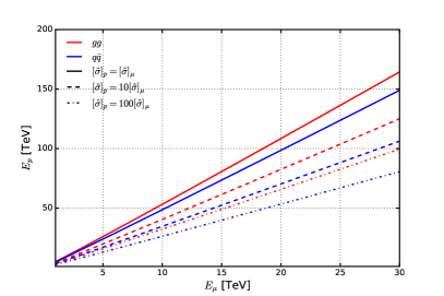
For various benchmark assumptions on the partonic cross sections and , and for the parton luminosity configurations (red) and (blue), where is any light quark, we plot in figure 1 the equivalent proton collider energy as a function of , for a generic , neutral current process. In particular, for each partonic configuration, we consider the case where the and partonic rates are the same, i.e., when (solid line) in equation 3.7, as well as when (dash) and (dash-dot). The purpose of these benchmarks is to cover various coupling regimes, such as when and are governed by the same physics or when is governed by, say, QCD but by QED .
Overall, we find several notable features. First is the general expectation that a larger collider energy is needed to achieve the same partonic cross section as a collider. This follows from the fact that beam energies are distributed among many partons whereas collider energies are effectively held by just two incoming partons. Interestingly, we find a surprisingly simple linear scaling between the two colliders for all and combinations. For the configuration and equal partonic coupling strength, i.e., , we report a scaling relationship of . Under the above assumptions, one would need a muon collider energy of to match the reach of a hadron collider with TeV. Specifically for the LHC and its potential upgrade to , one needs and , respectively. For the realistic case where the dynamics is ultra weakly coupled but dynamics is strong, i.e., , and proceeds through the partonic channel, we report a milder scaling of . This translates to needing a higher to achieve the same reach at a fixed . For example: for , one requires instead . As a cautionary note, we stress that the precise numerical values of scaling ratios reported here are somewhat accidental and can shift were one to assume alternative PDF sets or . The qualitative behavior, however, should remain.
3.2 annihilations
Instead of comparing the two colliders’ equivalent reach for processes, another possibility is to compare the reach for the pair production of heavy states. Doing so accounts for the nontrivial opening of new phase space configurations and kinematic thresholds. In the case, we assume that the muon collider is optimally configured, i.e., that is chosen slightly above threshold, where the production cross section is at its maximum. For collisions, the situation differs from the previous consideration in that pair production cross sections do not occur at fixed and, in general, are suppressed by , once far above threshold. Hence, we make the approximation that the quantity does not depend on , and recast beam-level cross sections in the following way:
| (3.8) | ||||
| (3.9) |
Assuming again that can be approximated by the -independent , and making analogous identifications as in equation 3.6, then after equating , we obtain
| (3.10) |
Here, the parton luminosity runs over the same configurations as in the case and similarly models the relationship between the (weighted) characteristic, partonic cross sections and . As in the previous case, we can solve equation 3.10 numerically (see footnote * ‣ 3.1) for the equivalent collider energy as a function of and .
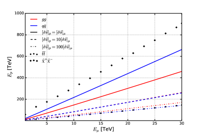
For the same benchmark assumptions on parton luminosities and partonic cross sections and as considered in figure 1, we plot in figure 1 the equivalent proton collider energy [TeV] as a function of [TeV], for a generic, , neutral current process. For concreteness, we also consider the LO production of top squark pairs through QCD currents in collisions but EW currents in collisions, as well as of chargino pairs through EW currents. For these cases, we fixed particle masses such that constitutes 90% of the total muon collider energy, i.e., .
As in the previous case, we again observe that a much higher energy collider exhibits the same reach as lower energy colliders. However, we find the scaling to be more drastic, with higher equivalent proton collider energies being reached for the same muon collider energies. We attribute this difference to the fact that, while a spectrum of is sampled in collisions, pair production beyond threshold is kinematically suppressed; this is unlike collisions where is fixed. Remarkably, we also find that the scaling relationship between and for processes retains its linear behavior for all our representative cases. In this measure of comparing colliders, we report a scaling relationship of for the configuration and equal partonic coupling strength, i.e., . This indicates that a muon collider of has roughly the same reach as a proton collider at . For the physics scenario where pair production is governed by weak (strong) dynamics in muon (proton), i.e., , we find very similar behavior for both the and parton configurations. As in the case, we report a smaller linear scaling of about , indicating that the reach of a hypothetical muon collider of can only exceed or match the reach of proton colliders up to .
For the concrete cases of stop (dot) and chargino (diamond) pair production, we observe several additional trends in figure 1. Starkly, we see that the scaling is in good agreement with the scenario where production is governed by ultra weak (strong) dynamics in muon (proton), i.e., , for the configuration. The preferred agreement for over follows from the production of high-mass states in collisions being typically driven by annihilation, where is a valence quark. For , we find poorer agreement with naïve scaling, with . This is about the estimation of the configuration with equal partonic coupling strength . We attribute this difference to the individual EW charges carried by elementary particles: as the coupling is suppressed, is dominated by the subchannel. The and couplings in , on the other hand, are more sizable, and interfere destructively with the subchannel, which itself is suppressed due to quarks’ fractional electric charge. This is unlike stop pair production since QCD and QED processes are less flavor dependent. The disagreement is hence tied to a breakdown of the assumption that are -independent. Nevertheless, we importantly find that our scaling relationships, as derived from equations 3.7 and 3.10, provide reliable, if not conservative, estimates for the equivalent collider energy for a given collider energy.
3.3 Weak boson fusion
We conclude this section by comparing the potential for EW VBF at high-energy and collider facilities. As we will analyze in the following sections, one of the main features of a multi-TeV lepton collider is the increased relevance of VBF over -channel scattering as the total collider energy increases. From this perspective, a muon collider could effectively be considered a “weak boson collider”. It is therefore interesting to compare the potential for VBF at a muon collider to that at a collider.
To make this comparison, we find it useful to continue in the language of parton luminosities and employ the Effective Approximation (EWA) [32, 33], which allows us to treat weak bosons on the same footing as QCD partons. That is to say, enabling us to consistently define parton luminosities in both and collisions. The validity of the EWA as an extension of standard collinear factorization in non-Abelian gauge theories [34] has long been discussed in literature [35, 36, 37, 19, 38]. More recent investigations have focused on reformulations that make power counting manifest [39, 40, 41] and matching prescriptions between the broken and unbroken phases of the EW theory [42, 43, 44].
Under the EWA, splitting functions are used to describe the likelihood of forward emissions of weak bosons off light, initial-state fermions. In the notation of equation 3.2, the helicity-dependent PDFs that describe the radiation of a weak vector boson in helicity state and carrying a longitudinal energy fraction from a fermion are [32, 33, 38]:
| (3.11) | ||||
| (3.12) |
Here and represent the appropriate weak gauge couplings of , given by
| (3.13) | |||||
| (3.14) |
At this order, the PDFs do not describe QED charge inversion, i.e., . For simplicity, we further define the spin-averaged transverse parton distribution as
| (3.15) |
For a lepton collider, the luminosities are defined as in equation 3.2, but with substituting the QCD parton PDFs with the weak boson PDFs . In particular, for in collisions for , we have
| (3.16) |
For the case, the luminosities are obtained after making the substitution
| (3.17) |
which is essentially the EW gauge boson PDF of the proton. The additional convolution accounts for the fact that in carries a variable momentum. (For simplicity, we keep all the same as in equation 3.2.) The luminosity at a scale in collisions is then,
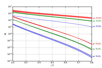
As a function of fractional scattering scale , where is the total collider energy and is the -system invariant mass, we plot in figure 2 the parton luminosities for (red), (green), (blue) in both (hatched shading) and (solid shading) collisions. Due to our choice to set the collinear factorization scale to half the partonic c.m. energy (see below equation 3.2 for details), the curves possess a (logarithmic) dependence on the collider energy. To take this ambiguity/dependency into account, we plot the envelopes for each parton luminosity spanned by varying for the proton (muon) case. The precise ranges of and that we consider help ensure that the partonic fraction of energy is neither too small nor too big, and hence that the EWA remains reliable [39]. We report that this “uncertainty” has little impact on our qualitative and quantitative assessments.
In figure 2, we find that for each helicity polarization configuration, the luminosity in collisions unambiguously exceeds the analogous luminosity in collisions over the considered. At , we find that the luminosities at a muon collider are roughly times those of a proton collider. Hence, for a fixed collider energy , the likelihood of scattering in collisions is much higher than for collisions. We attribute this to several factors: First is that the emerging EW PDFs in proton beams are a subdominant phenomenon in perturbation theory whereas in muon beams they arise at lowest order. Relatedly, as muons are point particles, they carry more energy than typical partons in a proton beam with the same beam energy. This enables EW PDFs in collisions to access smaller momentum fractions , thereby accessing larger PDF enhancements at smaller .
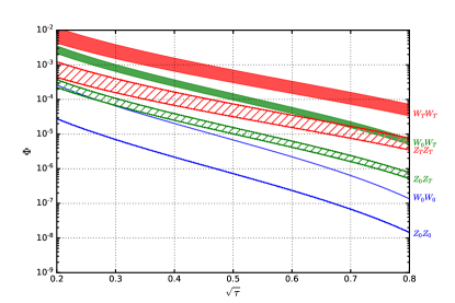
To further explore this hierarchy, we compare in figure 2 the collider luminosities for (solid shading) and (hatched shading) pairs, for (red), (green), and (blue). Globally, we see that the and luminosities exhibit a very similar shape dependence on , which follows from the functional form of . The normalization difference is due to the SU quantum number of muons, which results in the well-known suppression of couplings in the SM. Indeed, for , we find that the ratio of luminosities exhibits the constant relationship
| (3.19) |
While not shown, we report that the luminosities also have similar shapes and are located roughly at the geometric average of the and curves. Furthermore, due to gauge coupling universality, we anticipate that the luminosity hierarchy observed between muon and proton colliders extends to luminosities involving and bosons.
4 Standard Model processes at muon colliders
In this section we investigate and present cross sections for various EW boson and top quark final states of the form , where , and are integers that respectively denote the number of top quark pairs, weak vector bosons , and Higgs bosons . One of our goals of this survey is to systematically compare -channel annihilation processes with EW VBF production channels in collisions, and in particular identify the c.m. energies at which VBF rates overtake -channel ones.
Specifically, we consider VBF process as obtainable from a initial state. This consists of the sub-channels fusion (section 4.2), fusion (section 4.3), and fusion (section 4.4):
| ( fusion), | |
| ( fusion). | |
| ( fusion), |
We also consider collisions with same-sign muon pairs, (section 4.5). In this case, the and modes give rise to the same final state , up to charge multiplicities, at the same rate as collisions. The mode, on the other hand, opens truly new kinds of signatures while possessing the same luminosity as fusion reported in section 3. Before presenting our survey, we briefly comment in section 4.1 on a few technical details related to simulating many-particle final states in multi-TeV lepton collisions.
4.1 Technical nuances at high energies
An important issue in this study involves the fact that the final states above also receive contributions from non-VBF processes, like associated production of and a or boson. That is to say, from an -channel process but with an additional -strahlung emission that then splits into a lepton pair. In general, these contributions interfere with VBF topologies at the amplitude level and are not all separately gauge-invariant subprocesses. Therefore, in principle, they need to be considered together with VBF. However, the boson decay contributions are dominated by regions of phase space where are on their mass shells. Especially, at a lepton collider, where the initial-state energy of the collision is known accurately, such resonant configurations can be experimentally distinguished from the non-resonant continuum. In fact, the relative contributions of those resonant topologies as well as of their interference with the gauge-invariant VBF contributions are small when far from the on-shell region, i.e., where most of the VBF cross section is populated.
Therefore, in order to avoid double counting of results that we will present for -channel processes, as well as to make computations more efficient, we remove contributions with instances of on-shell , , and decays. In general, removing diagrams breaks gauge invariance and so we refrain from doing this. A simple solution, adopted for instance in Ref. [25], is to impose a minimum on the invariant mass of final-state lepton pairs. In this work, we adopt an even simpler prescription by simulating an initial state possessing a non-zero, net muon and electron flavor, i.e. collisions. In so doing, -channel annihilations are forbidden and VBF channels are automatically retained. We have checked for a few processes that the numerical differences with scattering rates of the analogous channels in the far off-shell region are small at high energies.
| [fb] | 1 TeV | 3 TeV | 14 TeV | 30 TeV | ||||
|---|---|---|---|---|---|---|---|---|
| VBF | s-ch. | VBF | s-ch. | VBF | s-ch. | VBF | s-ch | |
| 4.3 | 1.7 | 5.1 | 1.9 | 2.1 | 8.8 | 3.1 | 1.9 | |
| 1.6 | 4.6 | 1.1 | 1.6 | 1.3 | 1.8 | 2.8 | 5.4 | |
| 2.0 | 2.0 | 1.3 | 4.1 | 1.5 | 3.0 | 3.1 | 7.9 | |
| 4.8 | 1.4 | 2.8 | 3.4 | 1.1 | 1.3 | 3.0 | 5.8 | |
| 2.3 | 3.8 | 1.4 | 5.1 | 5.8 | 1.3 | 1.7 | 5.4 | |
| 7.1 | 3.6 | 3.5 | 3.0 | 1.0 | 5.3 | 2.7 | 1.9 | |
| 7.2 | 1.4 | 3.4 | 6.1 | 6.4 | 5.4 | 1.6 | 1.5 | |
| 5.1 | 5.4 | 6.8 | 6.7 | 1.1 | 2.5 | 2.1 | 1.0 | |
| 6.2 | 7.9 | 3.7 | 6.9 | 1.7 | 2.3 | 4.7 | 9.0 | |
| 2.1 | - | 5.0 | - | 9.4 | - | 1.2 | - | |
| 7.4 | - | 8.2 | - | 4.4 | - | 7.4 | - | |
| 3.7 | - | 3.0 | - | 7.1 | - | 1.9 | - | |
| 1.2 | 1.3 | 9.8 | 1.4 | 4.5 | 6.3 | 7.4 | 1.4 | |
| 1.5 | 1.2 | 9.4 | 3.3 | 1.4 | 3.7 | 3.3 | 1.1 | |
| 1.5 | 4.1 | 4.7 | 1.6 | 1.9 | 1.6 | 5.1 | 5.4 | |
| 8.9 | 3.8 | 3.0 | 1.1 | 3.4 | 1.3 | 7.6 | 4.1 | |
| 7.2 | 1.3 | 2.3 | 1.1 | 9.1 | 2.8 | 2.9 | 1.2 | |
| 2.7 | 3.2 | 1.2 | 8.2 | 1.6 | 8.8 | 3.7 | 2.5 | |
| 2.4 | 1.5 | 9.1 | 9.8 | 3.9 | 2.5 | 1.2 | 9.5 | |
| 1.6 | 2.7 | 1.2 | 4.7 | 5.3 | 3.2 | 8.5 | 8.3 | |
| 6.4 | 1.5 | 5.6 | 2.6 | 2.6 | 1.8 | 4.2 | 4.6 | |
| 1.1 | 5.9 | 4.1 | 3.3 | 5.0 | 6.3 | 1.0 | 2.3 | |
| 2.3 | 9.3 | 9.6 | 3.5 | 1.2 | 5.4 | 2.7 | 1.9 | |
A second technical issue that requires care is the treatment of unstable particles, and in particular the inclusion of fixed widths in Breit-Wigner propagators. While formally suppressed by for resonances of mass , these terms can break gauge invariance as well as spoil delicate unitarity cancellations at high energies. Indeed, we find that these disruptions can grow with energy for some processes and spoil the correctness of our calculations. A well-known solution is to consider the complex mass scheme [45, 46], an option that is available in mg5amc [26]. However, in this case, all unstable particles can only appear as internal states, not as external ones. This implies that when modeling each particle in our final state we always must include a decay channel (or decay channel chain), complicating our work considerably. Subsequently, we have opted for the solution of simulating external, on-shell with all widths set to zero. In doing so, gauge invariance is automatically preserved. Moreover, potential singularities in propagators are also automatically regulated due to their mass differences.
4.2 fusion
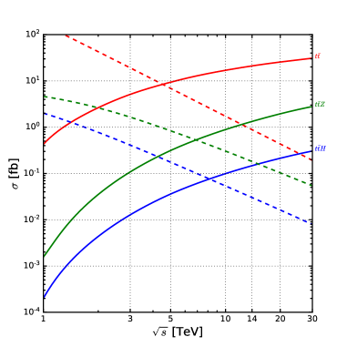
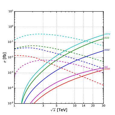
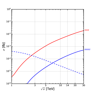
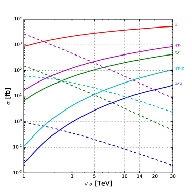
We begin our survey by considering the production of up to four heavy particles from fusion (solid lines) and -channel, annihilation (dashed lines). As a function of muon collider energy [TeV], we plot cross sections [fb] in figure 3 for (a) and (b) associated production. In figure 4 we plot the same for (a) , (b) , and (c) associated production, and (d) multiboson production. We summarize our findings in table 1 for representative collider energies and processes.
To summarize the global picture: as expected from the different production mechanism, -channel annihilation rates categorically scale and decrease with collider energy at least as , when collider energies are far beyond kinematic threshold. This is contrary to VBF processes where cross sections mildly increase with collider energy at least as a power of , in the high energy limit. Consequentially, we find that for all processes considered there is a where VBF production overcomes -channel production. In table 2 we report this and the corresponding at which the -channel and VBF cross sections are the same. In general, the larger the final state multiplicity, the larger the value of where the cross section curves cross. A few more remarks are in order.
First, for processes involving a top quark pair, as shown in figure 3, the -channel cross sections at lower energies of TeV are comparable to if not larger than those from VBF at TeV, i.e., the highest energy that we consider. In terms of statistics only, -channel annihilations at lower energies serve as a larger source of events. Hence, one may wonder if there is any gain in going to higher . This is addressed at length in section 5. Here it suffices to say that sensitivity to anomalous couplings greatly improves with increasing , in particular for VBF processes. For example: At lowest order, is only sensitive to anomalous and interactions; the channel is insensitive, e.g., to unitarity cancellations in the Higgs sector. This is unlike , which is also sensitive to anomalous , and couplings, including relative CP phases. In addition, the VBF channel features a strong, non-Abelian gauge cancellation, and therefore probes anomalous contributions that are enhanced by energy factors.
A second interesting observation is the hierarchy of production from fusion. As seen in figure 3, the rates for between systematically sit about an order of magnitude higher than , which in turn is another order of magnitude higher than . In fact, the rate sits just under the mixed EW-QCD rate, despite being less phase space-suppressed. We attribute the strong hierarchy to the relative minus signs among the top quark’s Yukawa coupling, the Higgs boson’s self-couplings, and the various weak gauge couplings, which together lead to large destructive interference.
Third, for processes involving neutral bosons and/or in the final state, VBF cross sections are systematically larger than -channel ones already at collider energies of a few TeV. This follows from the strong suppression of the gauge coupling relative to the unsuppressed gauge interaction. (Numerically, the further power of in fusion is still larger than the vector and axial-vector couplings of electrically charged leptons to bosons.) Among the processes investigated multi-Higgs production in VBF stands out. For the specific cases of annd production in figures 4 and 4, we find that VBF already exceeds -channel annihilation at and , respectively.
Lastly, the energy growth of VBF scattering rates is in general steeper for final states with larger particle multiplicities than for lower ones. This is due to many reasons. The first is that the increase in energy crucially opens phase space. For example: and have kinematic thresholds of and , indicating that their VBF production rates are phase space-starved for . The second relates to (collinear) logarithmic enhancements in processes with -channel gauge bosons. Final states with gauge bosons entail contributions from the exchange of -channel gauge bosons. At very high energies, such contributions become dominant and give rise to cross sections that behave at least as . Even though this largest log might not always be dominant, we verify that the growth pattern as a function of final-state multiplicity corresponds to this expectation and is rather clearly visible in plotted curves.
4.3 , , and fusion
| [fb] | 1 TeV | 3 TeV | 14 TeV | 30 TeV |
|---|---|---|---|---|
| 1.0 | 1.1 | 4.3 | 6.2 | |
| 1.2 | 6.7 | 5.2 | 8.5 | |
| 5.3 | 2.8 | 2.7 | 5.0 | |
| 1.5 | 3.8 | 7.6 | 9.6 | |
| 5.0 | 7.3 | 4.3 | 7.5 | |
| 3.6 | 3.1 | 8.4 | 2.3 | |
| 3.5 | 1.4 | 1.7 | 3.8 | |
| 2.5 | 4.9 | 3.6 | 5.9 | |
| 2.2 | 1.4 | 5.2 | 8.1 | |
| 1.2 | 4.0 | 7.4 | 8.0 |
We continue our survey at a potential multi-TeV facility by now exploring processes mediated through the neutral gauge bosons and . For a subset of final states considered in section 4.2 for fusion that can instead proceed through , , and fusion, we report in table 3 cross sections [fb] for representative collider energies. As described in section 4.1 we do not remove diagrams by hand and include interference. To regulate phase space singularities, a cut of 30 GeV is applied on outgoing charged leptons.
As foreseen from the scaling of the luminosity in section 3, the cross sections for fusion are smaller than for by roughly an order of magnitude. The exceptions to this are (i) production, which is highly comparable to the rate, and (ii) production, which is about two orders of magnitude smaller than . Despite being lower, these rates are not small enough to be neglected. Indeed, production already reaches ab at and grows to be as large as at . Moreover, the presence of final-state charged leptons from splittings, for example, could be exploited to obtain a full reconstruction of the event. For some particular channels it may also be useful to have charged lepton pairs to better identify a new resonance signal or increase sensitivity to an anomalous coupling. A simple but important example that is applicable to both the SM and BSM is the production of invisible final states, for example the SM process . Whereas the production mode would lead to a totally invisible final state, the mode gives a means to tag the process. Numerous BSM examples can also be constructed.
4.4 and scattering
| [fb] | 1 TeV | 3 TeV | 14 TeV | 30 TeV |
|---|---|---|---|---|
Turning away from final states with zero net electric charge, we now explore processes mediated by and fusion. For several representative processes, we summarize in table 4 their cross sections at our benchmark muon collider energies. We apply a cut of 30 GeV on outgoing charged leptons to regulate phase space singularities. Once again, following simple scaling arguments of the EWA luminosities in section 3, we expect and observe that cross sections here are somewhere between those of and fusion.
With the present VBF configuration, we find that the rates for , , and production (where ) all exceed the ab threshold at . At , the processes are strongly phase space-suppressed. At , we find that the and rates reach roughly the fb level and more than double at . Moreover, as the final states here are charged, the potential arises for qualitatively different signatures that cannot be produced via -channel annihilations. For example: processes such as single production (with pb), single top quark (with fb), as well as (with fb) all have appreciable cross sections for . If one assumes datasets, then in these cases, interesting, ultra rare and ultra exclusive decay channels can be studied.
4.5 fusion
Finally, we conclude our EW VBF survey by briefly exploring the case of same-sign muon collisions. This setup allows the production of doubly charged final states and therefore, as we discuss in section 6, is a natural setup where one can study lepton number-violating processes [47]. For concreteness, we consider collisions and in table 5 present the cross sections for representative and processes at our benchmark collider energies.
We report that the production rates for and are highly comparable to those for fusion in table 1. We anticipate this from CP invariance. This dictates that the luminosity in collisions is the same at lowest order as the luminosity in collisions. Differences between the two sets of rates originate from differences between the and analogous matrix elements. In scattering, only -channel exchanges of gauge and scalar bosons are allowed as there does not exist a doubly charged state in the EW sector. In scattering, these -channel diagrams interfere (constructively and destructively) with allowed -channel diagrams.
| [fb] | 1 TeV | 3 TeV | 14 TeV | 30 TeV |
|---|---|---|---|---|
| 2.2 | 1.4 | 5.6 | 9.0 | |
| 1.2 | 4.2 | 4.9 | 1.1 | |
| 9.3 | 3.1 | 3.7 | 8.5 |
5 Precision electroweak measurements
In this section we explore the potential of a muon collider to probe new physics indirectly. As it is not realistic to be exhaustive, after summarizing the effective field theory formalism in which we work (section 5.1), we select a few representative examples related to the Higgs boson (section 5.2) and the top quark (section 5.3).
5.1 SMEFT formalism
Undertaking precision measurements of SM observables is of utmost importance if nature features heavy resonances at mass scales that are just beyond the kinematic reach of laboratory experiments. Be it perturbative or non-perturbative, the dynamics of such new states could leave detectable imprints through their interactions among the SM particles. This is especially the case for the heaviest SM particles if the new physics under consideration is related to the flavor sector or the spontaneous breaking of EW symmetry.
Generically, two broad classes of observables, defined in different regions of phase space, can be investigated. The first are bulk, or inclusive, observables for which large statistics are available and even small deviations from the null (SM) hypothesis are detectable. The second are tail, or exclusive, observables, where the effects of new physics can be significantly enhanced by energy, say with selection cuts, and compensate for lower statistics.
A simple yet powerful approach to interpret indirect searches for new, heavy particles in low-energy observables is the SMEFT framework [22, 23, 24]. The formalism describes a large class of models featuring states that live above the EW scale and provides a consistent, quantum field theoretic description of deformations of SM interactions. This is done while employing a minimal set of assumptions on the underlying, ultraviolet theory. In SMEFT, new physics is parametrized through higher dimensional, i.e., irrelevant, operators that augment the unbroken SM Lagrangian, yet preserve the fundamental gauge symmetries of the SM by only admitting operators that are both built from SM fields and invariant under gauge transformations. Accidental symmetries of the SM, such as lepton and baryon number conservation, are automatically satisfied under certain stipulations [48, 49]. Additional global symmetries can also be imposed on the Lagrangian. In this work we assume the flavor symmetry,†††The labels refer, respectively, to the left-handed lepton doublets, the right-handed leptons, the right-handed down-type quarks, the right-handed up-type quarks, and the left-handed quark doublets. . This helps reduce the number of independent degrees of freedom while simultaneously singling out the top quark as a window onto new physics.
Under these assumptions, then after neglecting the Weinberg operator at dimension five and truncating the EFT expansion at dimension six, the SMEFT Lagrangian is
| (5.1) |
Here, are the dimensionless Wilson coefficients of the dimension-six operators . In the absence of additional symmetries, such as the flavor symmetry defined above, the number of independent stands at 59 if one considers only one generation of fermions and 2499 with three generations. In practice, one usually studies only a subset of operators in order to establish the sensitivity of a measurement. Since we are mainly interested in the top quark and Higgs sectors, we consequentially retain only operators that explicitly involve top or Higgs fields and affect EW observables. The full list of operators that we consider is given in table 6, where the following conventions are adopted:
| (5.2) | ||||
| (5.3) | ||||
| (5.4) |
Here, denotes the Pauli matrices, and is antisymmetric and normalized to unity.
| Operators | Limit on | Operators | Limit on | ||
|---|---|---|---|---|---|
| Individual | Marginalized | Individual | Marginalized | ||
| [-0.021,0.0055] [50] | [-0.45,0.50] [50] | [-5.3,1.6] [51] | [-60,10] [51] | ||
| [-0.78,1.44] [50] | [-1.24,16.2] [50] | [-7.09,4.68] [52] | |||
| [-0.0033,0.0031] [50] | [-0.13,0.21] [50] | [-0.4,0.2] [51] | [-1.8,0.9] [51] | ||
| [-0.0093,0.011] [50] | [-0.50,0.40] [50] | [-3.10,3.10] [52] | |||
| [-0.0051,0.0020] [50] | [-0.17,0.33] [50] | [-0.9,0.6] [51] | [-5.5,5.8] [51] | ||
| [-0.18,0.18] [53] | [-6.4,7.3] [51] | [-13,18] [51] | |||
5.2 Higgs self-couplings at muon colliders
A precise determination of the Higgs boson’s properties is one of the foremost priorities of the high-energy physics community [1, 2]. At the moment, measurements of the Higgs’s couplings to the heaviest fermions and gauge bosons are in full agreement with the SM predictions. However, there exist several couplings that have yet to be measured, and in some cases bounds are only weakly constraining. Among these are the Yukawa couplings to the first and second generation of fermions as well as the shape of the SM’s scalar potential. Subsequently, a determination of the Higgs’s trilinear and the quartic self-couplings, which are now fully predicted in the SM, would certainly help elucidate the EW symmetry breaking mechanism [54] and its role in the thermal history of the universe.
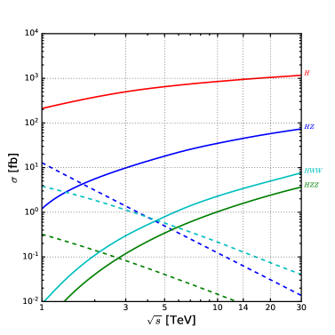
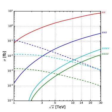
Despite this motivation, measurements of the Higgs’s self-interactions appears to be too challenging for the LHC, unless substantial deviations from the SM exist [55, 56, 57, 58, 59, 60, 61, 62, 63, 64, 65, 66, 67]. As such, conclusively measuring the Higgs’s properties is among the most compelling motivations for constructing a lepton collider at a c.m. energy of a few hundred GeV.‡‡‡It is remarkable that a 100 m radius circular muon collider could reach this energy [6]. The case for higher energies is also well-founded. For example: Higgs sensitivity studies for CLIC up to TeV [68, 69, 70, 71, 72, 73] support the expectation that increasing collider energy provides additional leverage for precision measurements through VBF channels. Indeed, as already shown in Fig. 4, VBF processes emerge as the dominant vehicles for and even production at high-energy lepton colliders and surpass -channel processes below TeV. Likewise, at TeV and with a benchmark luminosity of , one anticipates Higgs bosons in the SM [6]. As backgrounds are expected to be under good control, multi-TeV muon colliders essentially function as de facto Higgs factories.
Certainly, the limitations to extracting the Higgs’s self-couplings at the LHC and colliders motivate other opportunities, particularly those offered by muon colliders. However, past muon collider studies on the Higgs have been limited in scope, focusing largely on properties determination within the SM [11, 12, 14] and its minimal extensions [11, 13, 15]. Only recently have more robust, model-independent investigations been conducted [16, 25]. Expanding on this work, we perform in this section a first exploratory study on determining the SM’s full scalar potential in a model-independent fashion using SMEFT.
Within the SMEFT framework, three operators directly modify the Higgs potential:
| (5.5) |
The first contributes to the Higgs potential’s cubic and quartic terms and shifts the field’s (’s) vev . The latter two modify the Higgs boson’s kinetic term and a field redefinition is necessary to recover the canonical normalization. All of these operators give a contribution to VBF production of and through the following Lagrangian terms:
| (5.6) | |||
| (5.7) | |||
| (5.8) |
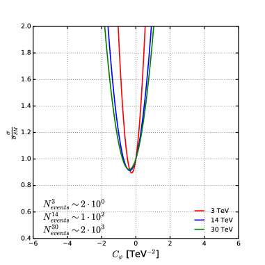
For conciseness, we investigate only the impact of and on prospective Higgs’s self-coupling measurements. We neglect since it also modifies couplings to gauge bosons and hence is already well-constrained by precision EW measurements. (See table 7 for details.) In the following, we consider a high-energy collider at a c.m. energy of , and 30 TeV, with respective benchmark luminosities , and 100 .
For the processes under consideration, we first discuss the impact of a single operator on inclusive cross sections while fixing all other higher dimensional Wilson coefficients to zero. Within the SMEFT, the total cross section of a process can be expressed by
| (5.9) |
Here the are the leading corrections in the power counting to the SM cross sections and are given by the interference between SM amplitudes and SMEFT amplitudes at . The corrections are the square contributions at , and come purely from SMEFT amplitudes at . The indices run through the set of operators that directly affect the process. We work under the assumption that the Wilson coefficients for operators in equation 5.5 are real. This indicates that the coefficients in correspond to and . As a naïve measure of the sensitivity to the dimension-six operators and considering only one operator at the time, we define the ratio
| (5.10) |
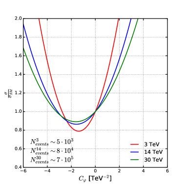
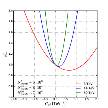
In figures 5 and 6, we respectively plot the sensitivity ratio, as defined in equation 5.10, for and production from VBF in collisions as a function of Wilson coefficients for operators (a) and (b) , for representative collider energies (red), (blue) and (green). Immediately, one sees that the two operators affect the ratio , and hence prospects for measuring the Higgs’s self couplings, in qualitatively different ways. To explore this, we first note that in equation 5.6 only shifts the Higgs’s trilinear and quartic couplings. The operator does not generate an additional energy dependence in the squared matrix element, apart from that which could be obtained by spoiling SM unitarity cancellations. As a result, the highest sensitivity to is reached near threshold production. Increasing actually results in losing sensitivity to production. Similarly for production, no significant impact on the cross section ratio is observed with increasing the collider energy, only a gain in the total number of events stemming from an increasing production rate. For the particular case of production at , the cross section is negligible and no measurement for this process can be undertaken. Independent of shifts to , it is important to point out that the higher the event rate the more feasible it becomes to study differential distributions of the above processes. Generically, an increased number of events allow us to more fully explore, and therefore exploit, regions of phase space that are more sensitive to BSM.
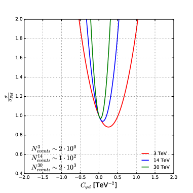
Contrary to , the operator introduces a kinematical dependence in interaction vertices. As a consequence, the impact of grows stronger and stronger as collider energy increases, potentially leading to a substantial gain in sensitivity. The imprint of this behavior is visible in the fact that the interference term between the SM and new physics becomes negligible as probing energy goes up. In this limit, the squared term dominates as naïvely expected from power counting at higher energies. This follows from the purely new physics contributions in SMEFT forcing to grow at most as , while the linear contributions force to grow at most as . Leaving aside questions of the EFT’s validity when corrections exceed those at , our point is that it is clear that sensitivity to and are driven by complementary phase space regions.
As a final comment, we would like to note that while the study of individual SMEFT operators can give important and useful information, in a realistic BSM scenario, multiple operators would simultaneously contribute to a given observable. In this more complicated scenario, correlations and numerical cancellations among operators appear, and phenomenological interpretations become more nuanced, more difficult. If we nevertheless put ourselves in the scenario where a measured cross section is consistent with the SM, then we can still define a simplified estimate of the experiment’s constraining power. In particular, we define the space of Wilson coefficients that predicts a cross section indistinguishable from SM expectation at the 95% confidence level (CL) by the following:
| (5.11) |
Here is the same SMEFT cross section as defined in equation 5.9. The number of background events is the SM expectation at a given luminosity , and the number of signal events is determined from the net difference between SMEFT and SM expectations.
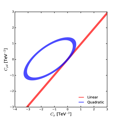
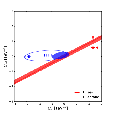
If we restrict ourselves to the two aforementioned operators, then equation 5.11 identifies an annulus or a disk in the 2D parameter space of Wilson coefficients. Hence, by combining observables one can gain constraining power by breaking such degeneracies. To see this explicitly, we show in Fig. 7 the 2D contour of allowed Wilson coefficients for and at (a) via production and (b) via both and production. (As mentioned above, the rate at 3 TeV is insignificant and hence omitted here.) Solutions to equation 5.11 are provided under the assumption that only linear corrections to are retained (red band) as well as when quadratic corrections are included (blue band). We also report the projected, marginalized limits on the two Wilson coefficients in table 8. Clearly, the lower energy machine leaves a much larger volume of parameter space unconstrained. In the 3 TeV case, the absence of a second measurement leads to a flat constraint in the linear case, which suggests an impossibility of conclusively constraining the parameter space. Moreover, this represents a strong case for measuring the triple Higgs production at lepton colliders in order to pin down the Higgs’s self-couplings. From this perspective, we argue that a TeV lepton (muon or electron) collider would be ideal over lower energy scenarios. Such a machine allows us to take advantage of both double and triple Higgs production, and at last measure the SM’s scalar potential.
It is important to point out that in order to have realistic assessments, one would need to perform a global study that includes multiple processes and operators together. In particular, while affects only and production, also shifts the coupling. This means that the total rate of single Higgs production is affected by and therefore one can constrain the corresponding Wilson coefficient. Even if the sensitivity to the operator is lower and does not grow with energy, the high statistics foreseen in multi-TeV lepton colliders is such that this operator will be heavily constrained by the inclusive measurement of single Higgs production. Assuming the aforementioned luminosities, we can estimate confidence level limits for to be roughly equal to at 3 TeV and at 14 TeV. Nonetheless, we found instructive to include this operator in the study, given the high sensitivity (see Fig. 5 and Fig. 6) caused by derivative couplings that lead to unitarity violating effects. Despite this, we notice that higher limits can be obtained in single Higgs production and therefore only (and potentially dimension 8 operators) will be relevant for and production.
In order to offer a comparison with other hypothetical future collider proposals, we quote here the projections from combined results at FCC-ee240, FCC-ee365, FCC-eh and FCC-hh, as reported in Ref. [73]. The first two are colliders with , at , respectively. The third is an collider with at , while the last is a collider with at . Under these scenarios, the projected individual bounds at 68% CL for operators we consider are
| (5.12) |
At a muon collider, we report that the anticipated sensitivity on the individual operators at 68% CL from measuring single Higgs production, as well as from double and triple Higgs production are
| (5.13) |
The difference is roughly a factor of for and a factor for . In the absence of production, the results here are comparable to those reported elsewhere [25]. This naïve comparison again shows the potential of a high-energy lepton collider in studying EW physics, allowing us to reach a precision that is certainly competitive with what attainable at other proposed colliders.
| 3 TeV | 14 TeV | |
| [-3.33, 0.65] | [-0.66, 0.23] | |
| [-1.31, 1.39] | [-0.17, 0.30] |
5.3 Top electroweak couplings at muon colliders
Due to its ultra heavy mass and complicated decay topologies, the era of precision top quark physics has only recently begun in earnest at the LHC. This is despite the particle’s discovery decades ago and rings particularly true for the quark’s neutral EW interactions [74]. For example: The associated production channel was only first observed using the entirety of the LHC’s Run I dataset [75, 76]. Likewise, the single top channel was observed only for the first time during the Run II program [77, 78]. And importantly, only recently has the direct observation of production process confirmed that the top quark’s Yukawa coupling to the Higgs boson is [79, 80, 81, 82, 83]. Since a precision program for measuring the top quark’s EW couplings is still in its infancy, there exists a margin for deviations from SM expectations. This makes it of stark importance to understand how to best measure these couplings, as searching for deviations could lead to new physics.
On this pretext, Ref. [84] studied a class of scattering processes involving the top quark and the EW sector within the SMEFT framework. There, the authors performed a systematic analysis of unitarity-violating effects induced by higher dimensional operators. By considering scattering amplitudes embedded in physical processes at present and future colliders, specific processes were identified that exhibited a distinct sensitivity to new physics. Among these processes, VBF at future lepton colliders stands out. The Wilson coefficients belonging to the operators in table 6 that impact VBF processes and involve the top quark are not strongly constrained. Hence, an improved measurement of these channels is important for the indirect tests of a plethora of BSM models.
In the context of a multi-TeV muon collider and following the proposal of Ref. [85], in this subsection we consider and compare the constraining potential of processes on anomalous couplings of the top quark. Even though such processes feature more complex Feynman diagram topologies and additional phase space suppression, their utility within the SMEFT framework stems from also featuring higher-point (higher-leg) contact interactions with a stronger power-law energy dependence at tree-level. In addition, a larger number of diagrammatic topologies translates into more possibilities to insert dimension-six operators, which, roughly speaking, may trigger larger deviations from the SM. (Though arguably larger cancellations are also possible.) For rather understandable limitations, such as finite computing resources, such considerations were not widely investigated before.
As an example, we consider the operator from table 6. For the case of scattering, this operator generates the four-point contact vertex
| (5.14) |
Here, one has to pay a vev penalty of , where the originates from the Higgs doublet , and thereby makes the term effectively a dimension-five contact term. On the other hand, by extending the final state with a Higgs field one can saturate the operator:
| (5.15) |
Remarkably, instead of , one is “penalized” by a factor of , where the energy dependence originates from the three-body phase space volume. This mechanism is rather generic and hence can be exploited for other operators and multiplicities in order to maximize the energy growth of amplitudes, and therefore the sensitivity to new physics.
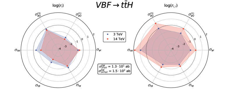
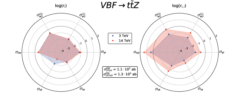
For concreteness, we compare the production of from VBF to the associated production of and from VBF. For each process we present in Fig. 8 the ratio coefficients and of as defined in equation 5.10, in the compact, radar plot format. More specifically, for several SMEFT operators (presented in the polar direction) we plot (left) the absolute value of the interference term at and (right) the quadratic term at in the radial direction (in logarithmic scale). We representatively fix each Wilson coefficient to TeV-2 and consider collider energies (blue dots) and (red dots). Contours at are bolded for clarity. Also reported in the figure are the total cross sections [fb] predicted in the SM.
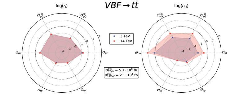
We observe in the case (Fig. 8) that the sensitivity to the operators under consideration is somewhat marginal. For both the linear (left) and quadratic (right) ratios deviations reach at most . The exception is , which features an term that can reach at . For all operators, linear contributions do not vary appreciably when passing from a c.m. energy of 3 TeV to 14 TeV. On the other hand, the quadratic terms exhibit an overall growth, just not a dramatic one. The smallness of contributions suggests that considering higher multiplicity processes, such as and , could prove more sensitive to new physics, despite naïve phase space suppression.
Adding a Higgs boson (Fig. 8) or a Z boson (Fig. 8) in the final state has a noticeable, quantitative impact on the overall behavior of ratio coefficients in the radar plots. When looking at the linear interference terms, it is surprising to see that many of the operators’ contributions decrease when going to higher energies. On the other hand, a sensitivity gain is unambiguous for all the operators in the quadratic case, which reach as much as . The behavior of interference is often more subtle to predict. Being non-positive definite, cancellations can and do readily take place depending on the specific phase space region that is considered. In particular, we infer that at higher energies these cancellations are enhanced, leading effectively to a lower sensitivity at the inclusive level.
Generically, each operator and process has a cancellation pattern of its own, which is also reinforced by the linear independence of SMEFT operators. Hence, designing a single recipe for every operator to invert cancellations with the aim of fully exploiting the increased sensitivity to energy is complicated. On the other hand, dedicated studies could lead to the discovery of a most sensitive (or a highly optimized) phase space region for a specific set of operators, enhancing the possibility to detect new physics.
While being more difficult to measure, these processes offer an overall improvement to sensitivity with respect to production of . This is both from the energy-growing perspective and from an absolute one. In essence, our very preliminary study here suggests that having a multi-TeV muon collider would benefit us for at least two reasons: (i) Due to phase space enhancements , a higher energy collider would allow us to take advantage of larger deviations from SM expectations, and hence higher sensitivity to SMEFT operators. (ii) The growth in the inclusive VBF cross section would allow us to have enough statistics to precisely measure higher multiplicity final states that would otherwise be infeasible even at . For example: we compare the events at 3 TeV to the at 14 TeV, assuming the benchmark luminosities considered ( and , respectively). The program to precisely determine the top quark’s EW interactions would therefore benefit greatly from a potential future muon collider by allowing us to take into account new processes that could help break degeneracies among SMEFT operators and learn about the dynamics of EW symmetry breaking.
6 Searches for new physics
Like hadron beams, muon beams emit significantly less synchrotron radiation than their electronic counterpart due to the muon’s much larger mass. As a result, colliders can reach partonic c.m. energies that far exceed conventional facilities, such as LEP II, and potentially even colliders; see section 3 for further details. Thus, in addition to the abundance of achievable SM measurements described in sections 4 and 5, a muon collider is able to explore new territory in the direct search for new physics.
In this section, we present a survey of BSM models and the potential sensitivity of a collider. Explicitly, we consider the -channel annihilation and VBF processes
| (6.1) |
Here, and is some BSM final state, which may include SM particles. We focus on the complementarity of the two processes because while -channel annihilation grants accesses to the highest available c.m. energies, it comes at the cost of a cross section suppression that scales as when far above production threshold. On the other hand, in VBF, the emission of transversely polarized, -channel bosons gives rise to logarithmic factors that grow with the available collider energy. Thus, VBF probes a continuum of mass scales while avoiding a strict -suppression, but at the cost of EW coupling suppression.
To investigate this interplay, for each scenario, we consider the mass and collider ranges:
| (6.2) |
We limit our study to due to the emergence of EW Sudakov logarithms in the VBF channels that scale as , for . These logarithms can potentially spoil the perturbative reliability of cross sections at LO and necessitate resummation of EW Sudakov factors [86, 42, 87, 88, 89]. While important for reliable predictions at higher , such resummation is beyond the present scope. For the various BSM scenarios, we assume benchmark values for relevant couplings. We omit generator-level phase space cuts where possible but stipulate them when needed to regulate matrix elements. In the following, we present the production rates of new processes. As a standard candle reference, in most scenarios, we also plot SM production via fusion (black, solid curve).
We start our survey in section 6.1 with minimally extending the SM by a scalar that is a singlet under the SM’s gauge symmetries. We then move onto the production of scalars in the context of the Two Higgs Doublet Model in section 6.2, and the Georgi-Machacek Model in section 6.3. In section 6.4, we investigate the production of sparticles in the context of the Minimal Supersymmetric Standard Model. We also consider representative phenomenological models describing the production of leptoquarks in section 6.5, heavy neutrinos in section 6.6, and vector-like quarks in section 6.7. We give an overview of this survey in section 6.8. A detailed comparison of -channel and VBF production mechanisms in BSM searches at multi-TeV muon colliders is deferred to section 7.
6.1 Scalar singlet extension of the Standard Model
The scalar sector of the SM consists of a single scalar doublet with a nonzero charge. While this is the minimal scalar content that supports the generation of fermion and weak boson masses through EWSB, the measured couplings of the Higgs boson uphold this picture [90, 91]. Theoretical motivation for extending this scalar sector, however, is well-established and the phenomenology of these scenarios have been studied extensively. For reviews, see Refs. [92, 93, 94, 95, 96, 97, 98] and references therein.
One of the simplest extensions that respects the SM symmetries is the addition of a single, real scalar that is neutral under all SM charges but carries an odd parity. Such scenarios have received recent attention [15, 16] as simplified models through which one can explore the sensitivity of multi-TeV muon colliders to new scalars. In light of LHC data, the phenomenology of a singlet scenario is categorized by whether acquires a nonzero vev: In the so-called inert scenario, does not acquire a vev, interacts at tree level only with the SM Higgs boson , and impacts ’s coupling to fermions and bosons at loop level [99]. If instead acquires a vev, then it mixes with the SM Higgs, which in turn modifies ’s coupling to SM particles at tree-level.


We investigate the muon collider sensitivity to the SM with an extra scalar singlet by considering the case where the vev of is nonzero, i.e., . The (unbroken) Lagrangian that describes such a scenario, including the symmetry, is given by
| (6.3) |
where is the full SM Lagrangian. After both the SM doublet and acquire their respective vevs, and , a mass-mixing term between and the neutral part of the doublet , and proportional to , is generated. Rotating and from the gauge basis and into the mass basis by an angle , we obtain the mass eigenstates and with mass eigenvalues and . The coupling of the lightest neutral scalar, which we assume is , to SM fermions and gauge bosons is suppressed relative to the SM by a factor of . Owing to strong constraints on anomalous Higgs couplings [90, 91], one scalar is aligned closely with the SM Higgs, which we assign to , implying . The bare parameters , can subsequently be exchanged for the physical parameters , which therefore permits us to express the trilinear scalar interactions as:
| (6.4) | |||||
| (6.5) | |||||
| (6.6) | |||||
| (6.7) |
The non-inert singlet scenario§§§Similarly, the inert singlet scenario is available using the SM_Plus_Scalars_UFO UFO libraries [100]. is implemented in the Minimal Dilaton Model UFO libraries by Ref. [101], and hence can be simulated using general purpose event generators.
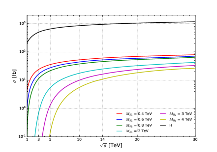
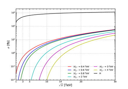
production in collisions can proceed through several mechanisms, including fusion, as shown in figure 9, which is mediated by an -channel boson. As shown above, for a given and , the coupling is related to the mass difference. Assuming the fixed, baseline mass splitting of Ref. [101], we show in figure 9 the pair production cross section [fb] via EW VBF as a function of collider energy [TeV].
In the numerical analysis we have assumed and . For , we see that the VBF process rate spans roughly fb for . For , we observe that the corresponding rates reach the order of fb at . By comparing these numbers with the SM productions of via VBF over the whole range of collider energies, we find that the latter are several order of magnitude larger, spanning fb.
6.2 Two Higgs Doublet Model

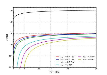
If a new neutral scalar does indeed exist, rather than being a SM singlet as posed in section 6.1, it may actually be a component of a second scalar doublet. Such scenarios, known in the literature as Two Higgs Doublet Models (2HDMs), have been extensively reviewed [92, 93, 102, 103], particularly for their necessity to realize Supersymmetry in nature. We consider the benchmark, CP-conserving 2HDM, the scalar potential of which is
| (6.8) |
Here, the couplings are real and the scalar doublets and are given by
| (6.9) |
After and/or acquire vacuum expectation values, EW is broken and fields with identical quantum numbers mix. More specifically, the charged scalars and neutral, CP-odd scalars mix into the EW Goldstone bosons and the physical states . Likewise, the neutral, CP-even scalars mix by an angle into the physical states and . Here, is identified as the observed, SM-like Higgs with and is heavier with . In terms of mass eigenstates, and are given explicitly by
| (6.10) |
Among the simplest processes we can analyze at a muon collider is resonant production of from fusion, which we show diagrammatically in figure 10. To estimate the sensitivity to this process, we consider the 2HDM in its CP-conserving scenario, as implemented in the 2HDM model file [104]. We show in figure 10 the production cross section [fb] via EW VBF as a function of collider energy [TeV] for representative mass . For , we find that cross sections span approximately fb for . For , we find that rates can reach several tens of fb at . Over the entire range of collider energies, we see that the SM production of is over an order of magnitude larger, reaching fb.
6.3 Georgi-Machacek Model
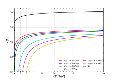
Another possibility at a future muon facility is the VBF production of electrically charged scalars. These, of course, do not exist in the SM nor in the simplest, naïve extensions of the SM scalar sector. In models such as the Georgi-Machacek (GM) model [105] and the Type II Seesaw model for neutrino masses [106, 107, 108, 109, 110], VBF production of singly charged and doubly charged scalars is possible due to the existence of scalar triplet representations of with nonzero hypercharge. (Higher representations also permit scalars with even larger electric charges.)
For present purposes, we focus on the feasibility of seeing exotically charged scalars from the GM model¶¶¶While it is also possible to model the Type II Seesaw with the TypeIISeesaw UFO libraries [111], we do not anticipate a qualitative difference in sensitivity from the GM case.. Broadly speaking, the model extends the SM with a real and a complex triplet with hypercharge and , respectively. If the vevs of the triplets’ neutral components are aligned, then tree-level, custodial symmetry is respected and strong constraints on the parameter are alleviated [92, 112, 113, 114, 115, 116, 117, 118]. More specifically, the GM scalar sector consists of the usual SM complex doublet with , a real triplet with , and a complex triplet with . Writing the doublet and triplets in the form of a bi-doublet and bi-triplet , we have
| (6.16) |


For our numerical results, we consider the decoupling limit of the GM model as implemented in the GM_UFO UFO [119, 120]. The (unbroken) scalar potential is given by
| (6.17) |
Here are the Pauli matrices. The matrices and are [119]
| (6.18) |
| (6.19) |
After aligning all states into their mass eigenstates, we are left with and , in addition to a number of neutral scalar and pseudoscalar states that we do not consider. In order to keep a consistent measure of collider sensitivity, we restrict ourselves to EW VBF production of and . In figure 11, we show a diagrammatic representation of the singly charged scalar produced resonantly through EW boson fusion, and present in figure 11 the production cross section [fb] as a function of collider energy [TeV] for representative masses . For relatively light , we find that resonant production rates are as low as fb at and can reach as high as fb at . For the relatively heavy , rates can reach up to several fb at the largest we consider. In figures 11 and 11, we show the same for in collisions. For the same mass and collider scales, we find that the resonant production rates of are a factor of a few larger than for . We attribute this to the fact that the coupling in the SM is larger than the coupling.
6.4 Minimal Supersymmetric Standard Model
In the SM, the Higgs boson possesses no symmetry that protects or stabilizes its mass against quantum corrections that naturally drive the mass away from the EW scale and toward the scale of new physics. As such, supersymmetric extensions of the SM (SUSY) are well-motivated theoretical scenarios. Under SUSY, the so-called hierarchy problem is softened or removed by hypothesizing that SM particles, along with missing members of a multiplet, belong to nontrivial representations of the Poincaré group [121, 122, 123, 124]. This leads to the existence of a new degree of freedom for each SM one that is mass-degenerate but with opposite spin-statistics, and that order-by-order contribute oppositely to quantum corrections of the Higgs’s mass. The lack of experimental evidence for superpartners [124, 125, 126, 127, 128, 129, 130, 131, 132, 133], however, suggests that if SUSY is realized at a certain scale it is broken at the EW scale.


While many variations of SUSY exist and are actively investigated, the Minimal Supersymmetric Standard Model (MSSM) is the simplest supersymmetric model supported by phenomenology [121, 122, 123, 124]. In it, the holomorphicity of the superpotential and anomaly cancellation require that two Higgs superfields be present (implying also that the MSSM is a supersymmetric extension of the 2HDM). The superpotential of the MSSM is given by
| (6.20) |
where , are the chiral superfields to which the Higgs and fermions belong. Apart from these terms are the vector superfields containing gauge bosons and gauginos as well as the Kähler potential, which describes particles’ kinetic terms. In studies and tests of the MSSM, one often also considers -parity, defined for each particle as
| (6.21) |
where , , and are the baryon number, lepton number, and spin of the particle. By construction, all SM particles (and 2HDM scalars) have , whereas their superpartners have . A consequence of parity is that the lightest supersymmetric particle is stable and, if it is electrically neutral, it is a good dark matter (DM) candidate.
Generically, scalar superpartners of quarks and leptons (squark and sleptons) with the same electric charge and color quantum numbers mix. In the MSSM, this results in two mixing matrices for the squarks (one each for the up and down sectors) and a mixing matrix for charged sleptons. (Neutrinos are natively massless in the MSSM as they are in the SM.) The neutral and charged superpartners of SM scalar and vector bosons also mix. The mass eigenstates, denoted by and , are given as linear combinations of the fields and , respectively. Despite extensive searches for these states [121, 122, 123, 124, 125], including direct searches at the LHC [126, 127, 128, 129, 130, 131, 132, 133], evidence for the MSSM at the weak scale has yet be established. If the MSSM, or any variation of SUSY, is realized at the EW- or TeV-scale, then a multi-TeV muon collider could be an optimal machine to discover missing superparticles or study the spectrum properties.
To investigate the sensitivity of muon colliders to the MSSM, we consider the benchmark, simplified scenario where generation-1 and -2 sfermions decouple while generation-3 squarks mix in pairs, and . We use the MSSM UFO libraries as developed by Ref. [134], and vary masses while keeping mass-splittings and couplings fixed.
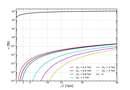
In figure 12 we show diagrammatically and numerically pair production of (a,b) top squarks, (c,d) neutralinos, and (c,d) charginos through VBF in collisions. Starting with figure 12, we have the production cross section [fb] as a function of [TeV], for representative stop masses. For lighter stops with , we see that cross sections span fb at and reach fb at . For heavier stops with , production rates reach fb at .
In figure 12, we show the same information but for . Overall, the picture is bleaker. For lighter neutralinos with , pair production rates through weak boson fusion remain below fb for collider energies below . They reach just below fb at . For heavier neutralinos with , we see that cross sections remain below fb for .
In figure 12, we again show the same information but for . We find that the outlook is somewhere between the previous cases. For lighter charginos with , pair production rates quickly reach about fb for and about fb at . For heavier charginos with , rates reach fb when , and span roughly fb for the highest considered.
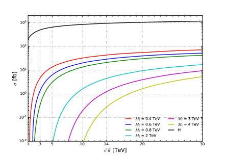
6.5 Vector leptoquarks

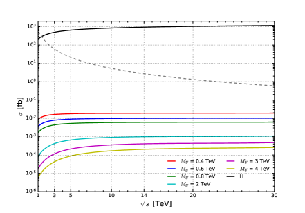
The existence of leptoquarks, i.e., scalar and vector bosons with nonzero baryon and lepton numbers, that also possess SM gauge charges have long been predicted due to their necessity in certain grand unified theories (GUTs) [135, 136, 137, 138, 139, 140, 141, 142]. Though not conclusively established [143, 125], the possibility of leptoquarks is a viable solution to longstanding anomalies observed across several flavor experiments [144, 145, 146, 147, 148, 149]. These anomalies suggest a violation of lepton flavor universality beyond what is allowed by neutrino oscillations. Hence, discovering and measuring properties of leptoquarks constitute an intriguing prospect at current and future experiments. For reviews on the topic, see Refs. [143, 150] and references therein.
While the spectrum of leptoquark models is vast, especially interesting options are those featuring vector leptoquarks due to their direct role in GUTs and recent demonstrations of their ultraviolet completions [151, 152, 153, 154]. For our purposes, we consider the concrete example [155] where the vector leptoquark arises from the enlarged gauge group
| (6.22) |
which itself is a subgroup of the Pati-Salam group [135]. In this case, is in the representation of the SM gauge group. At low energies, the relevant Lagrangian (before EWSB) can be described phenomenologically by [155]:
| (6.23) | ||||
Here, and are the QCD and hypercharge field strengths, with associated gauge couplings and . and are the field strength and mass of . and are anomalous couplings that vanish in gauged leptoquark models. are the SM chiral fermion fields in the flavor basis, and is a flavor-universal coupling strength while absorbs possible flavor dependencies.
In view of the aforementioned flavor anomalies, we assume that leptoquarks, if they indeed exist, couple mainly to generation-3 fermions with the possible extension to muons. Hence, to explore the sensitivity of multi-TeV muon colliders, we consider the process
| (6.24) |
mediated by a -channel exchange of the vector leptoquark , as shown in figure 13. We work in the framework of equation 6.23 as implemented into the LeptoQuark FeynRules UFO model [155]. For our purposes, the relevant parameters are and and we assume the default values of the model file. We report our results in figure 13, where we show the cross section [fb] as a function of collider energy [TeV] for representative . Also shown is the SM production rate (grey, dash curve). For both light and heavy masses, we observe only a mild dependence on collider energy. More specifically, for , we find cross sections are roughly fb for . For heavier masses in the range of , we see that cross sections span fb for collider energies of .
6.6 Heavy Dirac and Majorana neutrinos
In the SM, neutrinos are massless fermions. Neutrino oscillation data [156, 157], however, unambiguously demonstrate that they in fact possess exceptionally tiny masses, with eV [158]. If neutrinos are Majorana fermions, then their mass are also related to the breaking of lepton number conservation [159, 160, 161, 162], an accidental symmetry in the SM. In order to reconcile these observations with the SM paradigm, neutrino mass models, collectively known as Seesaw models, hypothesize the existence of new particles that necessarily [163] couple to SM leptons and the Higgs. If kinematically accessible, such states may be discovered at collider experiments through spectacular processes that violate lepton flavor and lepton number conservation; for comprehensive reviews, see Refs. [164, 47].
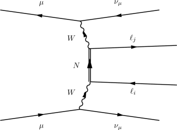
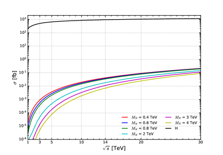
A commonality of many Seesaw models is the existence of heavy neutrino mass eigenstates that can be either (pseudo-)Dirac or Majorana. These states couple to the SM sector through mixing with SM neutrinos and/or new gauge couplings. For our purposes, we neglect subtleties related to decoupling of lepton number-violating processes in simplified models with only heavy neutrinos [165, 166, 162], and consider the well-studied [167, 168, 169] Phenomenological Type I Seesaw benchmark model, as implemented in the HeavyN UFO libraries of Ref. [170, 171]. In this model, neutrino flavor eigenstates can be expressed generically [168] in terms of light and heavy mass eigenstates by the decomposition
| (6.25) |
In the last expression we assumed that active-sterile mixing is dominated by the lightest, heavy mass eigenstate , which we relabel as . The relevant interaction Lagrangian coupling to the SM Weak bosons after EWSB is
| (6.26) | |||||
Here, is the coupling constant, is the weak mixing angle, and are the usual chiral projection operators for four-component fermions.
While there exists a number of processes in which heavy neutrinos can participate, we focus on the production of oppositely charged lepton pairs through scattering:
| (6.27) |
as show in figure 14. This signature complements conventional channel, including the -channel and processes and fusion, due to its particular sensitivity to active-sterile mixing, which scales as , and not requiring that be on-shell. Furthermore, observing this process for would give a clear indication of charged lepton flavor violation and provide guidance on the structure of neutrino mixing.
In figure 14, we show the cross section [fb] for the flavor-conserving process,
| (6.28) |
mediated by a heavy -channel neutrino, for representative mass , and as a function of collider energy [TeV]. For concreteness, we take . As in the leptoquark case in section 6.5, we observe only a slight rate dependence over a large range of neutrino masses. For , we find that cross sections reach the fb threshold at about . For much larger collider energies, we observe that scattering rates can reach up to fb for collider energies as large as .
6.7 Vector-like quarks
A more curious aspect of the SM is the existence of three copies, or generations, of matter. While at least three generations are necessary for CP violation in the quark sector [172], no first-principle argument establishes this to be the case. Moreover, as additional chiral generations are constrained by flavor and Higgs data [173, 174, 175], if more copies do exist, such matter particles likely belong to different EW representations or possess new quantum numbers. One such example: vector-like fermions, which are characterized by their left- and right-handed chiral components possessing identical gauge transformations but may nonetheless carry the same gauge charges as SM particles after EWSB.
As discussed in section 6.6, vector-like electrons and neutrinos are key ingredients of neutrino mass models. In addition, vector-like quarks (VLQ) offer viable, non-supersymmetric solutions to the Higgs mass hierarchy and dynamical EWSB [176, 177, 178]. The phenomenology of such models is rich, well-documented [179, 180, 181, 182, 183], and has led to LHC searches for vector-like top and bottom quarks in a variety of final states [184, 185, 186, 187, 188, 189].

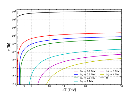
For fermionic top partners , i.e., a VLQ with the same quantum numbers as the top quark after EWSB, the effective Lagrangian describing can be parametrized by “decomposing” the top quark further into two mass eigenstate:
| (6.29) |
Here, is a small, model-dependent mixing parameter and the abuse of notation is obvious. While the Lorentz structure of the gluon and photon interactions with are dictated by gauge invariance, those of the EW bosons are less restricted. Generically, the EW couplings of a single with - and -flavored, SM quarks can be written as [183]:
| (6.30) |
Here, is the mass of the VLQ, is model-dependent and accounts for any potential flavor mixing, the index runs over the three SM generations, and the parameters (, , ) encode anomalous couplings to the EW bosons.
To investigate the sensitivity of multi-TeV muon colliders to VLQs, we consider pair production from fusion, as shown in figure 15 and given by
| (6.31) |
Using equation 6.30 as implemented in the VLQ UFO libraries by Ref. [183], we show in figure 15 the cross section [fb] in collisions as a function of collider energy [TeV], for representative . We assume the default couplings of Ref. [183].
Overall, we observe a large variation of production rates as a function of mass and collider energy. For lighter , with , we find that cross sections remain below the fb level for , but quickly grow with increasing . For the same mass range, rates reach roughly fb by . For heavier with , we see that the rate growth is milder, with the fb threshold achieved at . By , rates reach up to fb.
6.8 Overview of vector boson fusion sensitivity
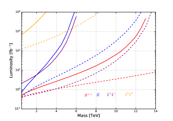
In this section we investigated the sensitivity of EW VBS to a variety of BSM scenarios at multi-TeV muon colliders. In order to give an overview picture of this reach, we present in figure 16 the requisite integrated luminosity [fb-1] for a discovery as a function of new particle mass in (solid) and (dashed) muon collisions. We consider specifically the doubly charged Higgs (red) from the GM model (see section 6.3); (blue), (purple), and (yellow) pairs from the MSSM (see section 6.4). As dedicated signal and background analyses are beyond the scope of this document, we crudely assume a zero background hypothesis and full signal acceptance. We therefore also use as a simple measure of statistical significance the formula, .
As a general feature, we see that less integrated luminosity is needed to achieve the same discovery at higher collider energies (dashed lines) than is needed at lower collider energies (solid lines). For example: For pair production with , about at are needed to reach . Similarly, for pair production with TeV, one can pass the threshold with roughly . For of mass , one would need about at .
While highly intuitive for colliders, this behavior is somewhat a novelty for lepton colliders because typical, -channel annihilation processes exhibit cross sections that decrease with increasing collider energy. Hence, for -channel annihilations, one typically needs more data at higher collider energies to achieve the same discovery potential. We attribute this improved outlook to the increasing likelihood for forward, initial-state EW boson radiation at higher collider energies. That is to say, the opening and increasing importance of EW vector boson fusion channels. In terms of the parton luminosity language of section 3, a higher collider energy translates to a larger EW boson parton luminosity. For a fixed “partonic” scattering rate, this leads to an increased, beam-level cross section, and therefore higher sensitivity. In this sense, multi-TeV lepton colliders start resembling proton colliders, and effectively become high-luminosity, weak boson colliders. While remaining in the context of the above BSM scenarios, we now explore this perspective further.
7 New physics processes at muon colliders: annihilation vs fusion
As we have shown here and throughout previous sections, VBF production cross sections grow with increasing , a phenomenon that follows from the propensity for forward emission of transverse gauge bosons at increasing collider energies. While the precise dependence of on collider energies of course depends on the precise BSM signature, for example on the particles involved, their underlying dynamics, and their kinematics, it nevertheless contrasts with -channel, annihilation processes. These processes feature cross sections that instead decrease with collider energy as , when well above kinematic thresholds. Hence, just as in the SM, we find a commonality in all VBF process here: assuming fixed model inputs, then for sufficiently high collider energies, VBF cross sections exceed those of analogous, -channel production modes.
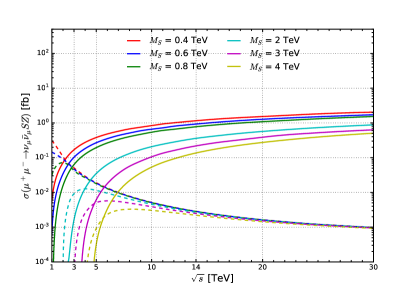
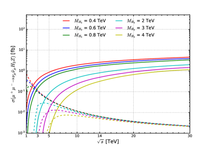
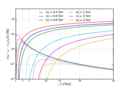
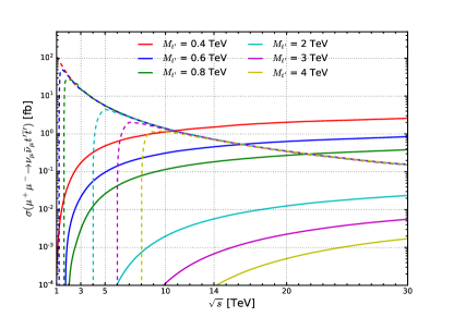
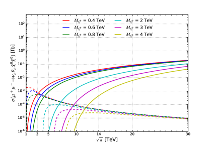
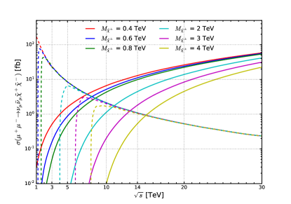
As in the SM case studies of section 4, there is not a definite energy beyond which -channel, annihilations are categorically subdominant. The situation is more nuanced. For example: as in our SM cases, the more final-state particles involved, the larger the needed for to exceed . For the resonant production of BSM states, there is of course another important parameter that plays a role: the mass scale of new, final state particle(s). New mass scales complicates the naïve scaling for VBS in two ways. First is the aforementioned propensity for collinear emission of transverse gauge bosons, which, more precisely, grows with the invariant mass of the VBF system. Second is the possible enhancement of “soft” EW boson emissions at small momentum fractions. Third is the role of matrix elements featuring large longitudinal gauge boson couplings that nevertheless possess a relatively suppressed parton luminosity (see section 3.3).
To explore how the mass scale of new particles impacts the threshold at which surpasses , and working in the context of the BSM scenarios of section 6, we compare in figure 17 a variety of VBF and analogous -channel, annihilation processes in multi-TeV collisions. Assuming representative input parameters and as a function of muon collider energy [TeV], we show the VBF (solid lines) and -channel (dashed lines) cross sections for: 17 associated production in a singlet-scalar extension of the SM (see section 6.1); 17 associated production in the 2HDM (see section 6.2); 17 , 17 , and 17 pair production in the MSSM (see section 6.4); as well as 17 pair production in a vector-like quark scenario (see section 6.7). Estimated collider energies at which the VBF rates surpass the -channel rates are summarized in Table 9.
From this exercise we observe several trends. We start by noting that the VBF production rates supersede -channel rates at relatively lower collider energies for , , , and production than for and pair production. In particular, for and , we report that becomes larger than at around for . For heavier masses of , the transition energies both span . The same mass dependence can be found for and production. For the same ranges of lighter and heavier masses, the VBF cross sections become prevalent at and . The two sets of processes can further be linked by noting that the benchmark masses probe approximately the same scales as the benchmarks, with reasonable consistency. This trend suggests some universal-like scaling behavior.
| mass [TeV] | (Singlet) | (2HDM) | (VLQ) | (MSSM) | (MSSM) | (MSSM) | Scaling (Eq. 7.7) |
|---|---|---|---|---|---|---|---|
| 400 GeV | 2.1 TeV | 2.1 TeV | 11 TeV | 2.9 TeV | 3.2 TeV | 7.5 TeV | 1.0 (1.7) TeV |
| 600 GeV | 2.5 TeV | 2.5 TeV | 16 TeV | 3.8 TeV | 3.8 TeV | 8.1 TeV | 1.3 (2.4) TeV |
| 800 GeV | 2.8 TeV | 2.8 TeV | 22 TeV | 4.3 TeV | 4.3 TeV | 8.5 TeV | 1.7 (3.1) TeV |
| 2.0 TeV | 4.0 TeV | 4.0 TeV | >30 TeV | 7.8 TeV | 6.9 TeV | 11 TeV | 3.7 (6.8) TeV |
| 3.0 TeV | 4.8 TeV | 4.8 TeV | >30 TeV | 10 TeV | 9.0 TeV | 13 TeV | 5.3 (9.8) TeV |
| 4.0 TeV | 5.5 TeV | 5.5 TeV | >30 TeV | 13 TeV | 11 TeV | 15 TeV | 6.8 (13) TeV |
For pair production of and , we find that the VBF channels become more important than -channel production at much higher collider energies than the previously discussed processes. More specifically, for , we find that collider energies must exceed TeV for lighter (heavier) mass scales. For , the outlook is even worse. We find that VBF production only becomes important for for relatively light masses of , whereas for heavier masses of , one requires collider energies that exceed .
We attribute the qualitative differences between these two processes and the previous four processes to differences between subprocesses in the -channel and VBF mechanisms. In the first four cases, both -channel and VBF proceed largely through the same EW gauge interactions. In the latter two cases, the -channel and VBF channels differ by additional -channel exchanges that are governed not by gauge couplings but by mixing factors and Yukawa couplings. The crossover, then, exhibits a stronger model dependency when VBF and -channel diagrams adhere to different dynamics or interaction strengths.
As already stated, for the , , , and channels, we observe a suggestive, universal-like behavior at which the VBF cross sections surpass their -channel counter parts for a given final-state mass scale . This behavior can be roughly estimated by noting that the kinematic scaling for , -channel cross sections are of the form
| (7.1) |
The denominator takes its form from the propagator of some intermediate state of mass (it make no difference which state), and the numerator from momentum conservation, which requires the cross section to vanish when the collider energy dips to the mass threshold of the final-state. Likewise, the differential rate for VBF processes that (importantly) proceed through the same interactions as -channel process scale as
| (7.2) |
Here we use the Effective Approximation (see section 3.3) to model the hard process, which is mediated by EW bosons carrying energy fractions . (We make implicit a summation over all permutations that contribute to .) In the final step, we assume that the invariant mass of the -system is large, i.e., , and express the scaling in terms of equation 7.1. Now, as seen in equation 3.11, the EWA PDFs contribute largest at small momentum fractions , i.e., the limit where gauge radiation goes soft. Moreover, as shown in figure 2, the luminosity is dominated by transverse polarizations. Hence, in the small- limit (and setting the factorization scale ), the leading contribution to equation 7.2 scales as
| (7.3) |
Here we introduce explicitly a multiplicity factor to account for (sum) the four transverse polarization permutations that contribute to production.
If we make the strong assumption that the -system’s mass is also large in comparison to , then the VBF scaling, in terms of the -channel scaling, simplifies to
| (7.4) |
where is the dimensionless scale at which proceeds, and is the smallest at which the hard process can kinematically occur. In the first step, we group collinear logs under the stipulation that the mass difference is negligible. In the second, we made a change of variable to express the momentum integrals in terms of traditional collider variables. After integrating and in terms of the -channel scaling, the VBF dependence on collider energy for scales as
| (7.5) | |||||
| (7.6) |
We observe that the scaling behavior for VBF processes exhibits a double collinear logarithmic dependence on , which stems from two collinear, EW PDFs, but remarkably only a single soft logarithm. The double soft logarithm does not arise as the hard process is power-suppressed by a relative factor of . This in turn manifests as a power-law factor that grows linearly with .
Altogether, this enables us to roughly estimate the collider energy at which surpasses for a given final-state mass . Essentially, one must solve for when
| (7.7) |
While the result is transcendental, the solution can easily be extracted numerically∥∥∥Explicitly, we use the Mathematica function NSolve and report very quick runtime on a personal laptop. for the representative , which we report in the rightmost column of Table 9 assuming a mass scale . For sub-TeV masses, the scaling behavior systematically underestimates the true crossover by roughly a factor of two. This is unsurprising as equation 7.7 assumes a large hierarchy between relevant scales. For TeV masses and above, however, we find good agreement between equation 7.7 and explicit computation from Monte Carlo computations. We report differences ranging from the percent level to the 20% level.
8 Conclusions
The next generation of particle accelerators needed to explore the energy frontier will offer tremendous challenges. Among these is a muon collider running at energies up to several TeVs and luminosities in the tens of inverse attobarns, a dream machine both from the technology and physics points of view. Overcoming the challenges posed by producing, storing, and colliding high-intensity beams of high-energy muons will take years of further research and development. Exploring the physics potential of such machines, on the other hand, is a relatively easy task that can be undertaken on a short time scale.
In this paper, we have moved a small step forward in the latter direction by considering electroweak vector boson fusion/scattering (VBF) processes at a future multi-TeV lepton collider in a rather systematic way. Our study is motivated by the simple observation that while -channel production rates decrease with increasing collider energy as , VBF rates grow as a power of , and therefore, for any final state, VBF is consigned to eventually emerge as the leading production mechanism.
In this context, we have investigated and show in section 3 that, compared to hadron colliders, VBF is a much more relevant production mechanism at a high-energy lepton collider. We continue in section 4 and present for a rather large set of SM final states involving EW vector bosons, Higgs bosons, and top quarks the corresponding VBF cross sections and at what collider energy they surpass -channel production modes. We find that VBF becomes the dominant production mechanism at relatively low collider energies, starting at just a few TeV for low final-state multiplicities and increases for higher multiplicities.
In order to further illustrate what could be attainable in terms of new physics reach, we then moved in two directions, focusing mostly on luminosity scenarios envisaged for a muon collider. First, in section 5, we considered prospects for precision measurements of the Higgs’s self-couplings and the top quark’s EW couplings, and interpreted sensitivity in terms of Wilson coefficients within the SMEFT framework. Second, in section 6, we explored a variety of simplified extensions of the SM and how large VBF luminosities can maximize the direct search for new physics. In particular we find evidence that in several instances the reach of a multi-TeV muon collider is comparable or better than that attainable at a 100 TeV proton-proton collider. A detailed comparison of VBF’s utility over -channel annihilations in BSM searches was then summarized in section 7.
The results presented in this work are meant to provide a first glimpse of what could be achieved at a multi-TeV muon collider in VBF channels, and certainly motivate further and more refined investigations. We close by stressing that while we focus on the specific prospects of a muon collider, our conclusions hold equally for other lepton colliders.
Acknowledgements
FM, LM, and XZ would like to thank Mauro Chiesa, Roberto Franceschini, Barbara Mele and Fulvio Piccinini for many discussions on the physics of muon colliders. RR thanks Carlos Alishaan for helpful discussions.
This work has received funding from the European Union’s Horizon 2020 research and innovation programme as part of the Marie Skłodowska-Curie Innovative Training Network MCnetITN3 (grant agreement no. 722104), FNRS “Excellence of Science” EOS be.h Project No. 30820817. The work of AC is supported by INFN research grant n. 20286/2018. RR is supported under the UCLouvain fund “MOVE-IN Louvain” and acknowledge the contribution of the VBSCan COST Action CA16108.
Computational resources have been provided by the supercomputing facilities of the Université catholique de Louvain (CISM/UCL) and the Consortium des Équipements de Calcul Intensif en Fédération Wallonie Bruxelles (CÉCI) funded by the Fond de la Recherche Scientifique de Belgique (F.R.S.-FNRS) under convention 2.5020.11 and by the Walloon Region.
References
- [1] R. K. Ellis and others (European Strategy for Particle Physics Preparatory Group), Physics Briefing Book: Input for the European Strategy for Particle Physics Update 2020, 1910.11775.
- [2] European Strategy Group collaboration, 2020 Update of the European Strategy for Particle Physics. CERN Council, Geneva, 2020, 10.17181/ESU2020.
- [3] AWAKE collaboration, E. Gschwendtner et al., AWAKE, The Advanced Proton Driven Plasma Wakefield Acceleration Experiment at CERN, Nucl. Instrum. Meth. A829 (2016) 76–82, [1512.05498].
- [4] R. Palmer et al., Muon collider design, Nucl. Phys. Proc. Suppl. 51A (1996) 61–84, [acc-phys/9604001].
- [5] C. M. Ankenbrandt et al., Status of muon collider research and development and future plans, Phys. Rev. ST Accel. Beams 2 (1999) 081001, [physics/9901022].
- [6] J. P. Delahaye, M. Diemoz, K. Long, B. Mansoulié, N. Pastrone, L. Rivkin et al., Muon Colliders, 1901.06150.
- [7] R. B. Palmer, Muon Colliders, Rev. Accel. Sci. Tech. 7 (2014) 137–159.
- [8] M. Antonelli and P. Raimondi, Snowmass Report: Ideas for Muon Production from Positron Beam Interaction on a Plasma Target, in Proceedings, 2013 Community Summer Study on the Future of U.S. Particle Physics: Snowmass on the Mississippi (CSS2013): Minneapolis, MN, USA, July 29-August 6, 2013, 2013, http://www.lnf.infn.it/sis/preprint/detail-new.php?id=5331.
- [9] M. Antonelli, M. Boscolo, R. Di Nardo and P. Raimondi, Novel proposal for a low emittance muon beam using positron beam on target, Nucl. Instrum. Meth. A807 (2016) 101–107, [1509.04454].
- [10] N. Bartosik et al., Preliminary Report on the Study of Beam-Induced Background Effects at a Muon Collider, 1905.03725.
- [11] V. D. Barger, M. S. Berger, J. F. Gunion and T. Han, s channel Higgs boson production at a muon muon collider, Phys. Rev. Lett. 75 (1995) 1462–1465, [hep-ph/9504330].
- [12] T. Han and Z. Liu, Potential precision of a direct measurement of the Higgs boson total width at a muon collider, Phys. Rev. D 87 (2013) 033007, [1210.7803].
- [13] N. Chakrabarty, T. Han, Z. Liu and B. Mukhopadhyaya, Radiative Return for Heavy Higgs Boson at a Muon Collider, Phys. Rev. D 91 (2015) 015008, [1408.5912].
- [14] M. Greco, T. Han and Z. Liu, ISR effects for resonant Higgs production at future lepton colliders, vol. 763, pp. 409–415. 12, 2016. 1607.03210. 10.1016/j.physletb.2016.10.078.
- [15] D. Buttazzo, D. Redigolo, F. Sala and A. Tesi, Fusing Vectors into Scalars at High Energy Lepton Colliders, JHEP 11 (2018) 144, [1807.04743].
- [16] M. Ruhdorfer, E. Salvioni and A. Weiler, A Global View of the Off-Shell Higgs Portal, SciPost Phys. 8 (2020) 027, [1910.04170].
- [17] S. Dawson and J. L. Rosner, Capabilities of Collisions for Producing Very Heavy Higgs Bosons, Phys. Lett. B 148 (1984) 497–501.
- [18] K.-i. Hikasa, Heavy Higgs Production in and Collisions, Phys. Lett. B 164 (1985) 385. [Erratum: Phys.Lett.B 195, 623 (1987)].
- [19] G. Altarelli, B. Mele and F. Pitolli, Heavy Higgs Production at Future Colliders, Nucl. Phys. B287 (1987) 205–224.
- [20] W. Kilian, M. Kramer and P. Zerwas, Higgsstrahlung and W W fusion in e+ e- collisions, Phys. Lett. B 373 (1996) 135–140, [hep-ph/9512355].
- [21] J. Gunion, T. Han and R. Sobey, Measuring the coupling of a Higgs boson to Z Z at linear colliders, Phys. Lett. B 429 (1998) 79–86, [hep-ph/9801317].
- [22] B. Grzadkowski, M. Iskrzynski, M. Misiak and J. Rosiek, Dimension-Six Terms in the Standard Model Lagrangian, JHEP 10 (2010) 085, [1008.4884].
- [23] J. Aebischer et al., WCxf: an exchange format for Wilson coefficients beyond the Standard Model, Comput. Phys. Commun. 232 (2018) 71–83, [1712.05298].
- [24] I. Brivio, Y. Jiang and M. Trott, The SMEFTsim package, theory and tools, JHEP 12 (2017) 070, [1709.06492].
- [25] M. Chiesa, F. Maltoni, L. Mantani, B. Mele, F. Piccinini and X. Zhao, Measuring the quartic Higgs self-coupling at a multi-TeV muon collider, 2003.13628.
- [26] J. Alwall, R. Frederix, S. Frixione, V. Hirschi, F. Maltoni, O. Mattelaer et al., The automated computation of tree-level and next-to-leading order differential cross sections, and their matching to parton shower simulations, JHEP 07 (2014) 079, [1405.0301].
- [27] NNPDF collaboration, R. D. Ball et al., Parton distributions for the LHC Run II, JHEP 04 (2015) 040, [1410.8849].
- [28] A. Buckley, J. Ferrando, S. Lloyd, K. Nordström, B. Page, M. Rüfenacht et al., LHAPDF6: parton density access in the LHC precision era, Eur. Phys. J. C75 (2015) 132, [1412.7420].
- [29] W. Kilian, T. Ohl and J. Reuter, WHIZARD: Simulating Multi-Particle Processes at LHC and ILC, Eur. Phys. J. C71 (2011) 1742, [0708.4233].
- [30] A. Denner, J.-N. Lang and S. Uccirati, Recola2: REcursive Computation of One-Loop Amplitudes 2, Comput. Phys. Commun. 224 (2018) 346–361, [1711.07388].
- [31] C. Quigg, LHC Physics Potential versus Energy, 0908.3660.
- [32] S. Dawson, The Effective W Approximation, Nucl. Phys. B249 (1985) 42–60.
- [33] G. L. Kane, W. W. Repko and W. B. Rolnick, The Effective W+-, Z0 Approximation for High-Energy Collisions, Phys. Lett. 148B (1984) 367–372.
- [34] J. Collins, Foundations of perturbative QCD, Camb. Monogr. Part. Phys. Nucl. Phys. Cosmol. 32 (2011) 1–624.
- [35] R. N. Cahn, Production of Heavy Higgs Bosons: Comparisons of Exact and Approximate Results, Nucl. Phys. B255 (1985) 341. [Erratum: Nucl. Phys.B262,744(1985)].
- [36] S. S. D. Willenbrock and D. A. Dicus, Production of Heavy Quarks from W Gluon Fusion, Phys. Rev. D34 (1986) 155.
- [37] S. Dawson and S. S. D. Willenbrock, Heavy Fermion Production in the Effective Approximation, Nucl. Phys. B284 (1987) 449.
- [38] Z. Kunszt and D. E. Soper, On the Validity of the Effective Approximation, Nucl. Phys. B296 (1988) 253–289.
- [39] P. Borel, R. Franceschini, R. Rattazzi and A. Wulzer, Probing the Scattering of Equivalent Electroweak Bosons, JHEP 06 (2012) 122, [1202.1904].
- [40] A. Wulzer, An Equivalent Gauge and the Equivalence Theorem, Nucl. Phys. B885 (2014) 97–126, [1309.6055].
- [41] J. Chen, On the Feynman Rules of Massive Gauge Theory in Physical Gauges, 1902.06738.
- [42] J. Chen, T. Han and B. Tweedie, Electroweak Splitting Functions and High Energy Showering, JHEP 11 (2017) 093, [1611.00788].
- [43] J. Chen, Electroweak Splitting Functions and High Energy Showering, Ph.D. thesis, U. Pittsburgh (main), 2017.
- [44] G. Cuomo, L. Vecchi and A. Wulzer, Goldstone Equivalence and High Energy Electroweak Physics, SciPost Phys. 8 (2020) 078, [1911.12366].
- [45] A. Denner, S. Dittmaier, M. Roth and D. Wackeroth, Predictions for all processes e+ e- —> 4 fermions + gamma, Nucl. Phys. B560 (1999) 33–65, [hep-ph/9904472].
- [46] A. Denner, S. Dittmaier, M. Roth and L. H. Wieders, Electroweak corrections to charged-current e+ e- —> 4 fermion processes: Technical details and further results, Nucl. Phys. B724 (2005) 247–294, [hep-ph/0505042]. [Erratum: Nucl. Phys.B854,504(2012)].
- [47] Y. Cai, T. Han, T. Li and R. Ruiz, Lepton Number Violation: Seesaw Models and Their Collider Tests, Front.in Phys. 6 (2018) 40, [1711.02180].
- [48] A. Kobach, Baryon Number, Lepton Number, and Operator Dimension in the Standard Model, Phys. Lett. B758 (2016) 455–457, [1604.05726].
- [49] A. Helset and A. Kobach, Baryon Number, Lepton Number, and Operator Dimension in the SMEFT with Flavor Symmetries, Phys. Lett. B800 (2020) 135132, [1909.05853].
- [50] J. Ellis, C. W. Murphy, V. Sanz and T. You, Updated Global SMEFT Fit to Higgs, Diboson and Electroweak Data, JHEP 06 (2018) 146, [1803.03252].
- [51] N. P. Hartland, F. Maltoni, E. R. Nocera, J. Rojo, E. Slade, E. Vryonidou et al., A Monte Carlo global analysis of the Standard Model Effective Field Theory: the top quark sector, JHEP 04 (2019) 100, [1901.05965].
- [52] A. Buckley, C. Englert, J. Ferrando, D. J. Miller, L. Moore, M. Russell et al., Constraining top quark effective theory in the LHC Run II era, JHEP 04 (2016) 015, [1512.03360].
- [53] A. Butter, O. J. P. Éboli, J. Gonzalez-Fraile, M. C. Gonzalez-Garcia, T. Plehn and M. Rauch, The Gauge-Higgs Legacy of the LHC Run I, JHEP 07 (2016) 152, [1604.03105].
- [54] D. J. H. Chung, A. J. Long and L.-T. Wang, 125 GeV Higgs boson and electroweak phase transition model classes, Phys. Rev. D87 (2013) 023509, [1209.1819].
- [55] CMS collaboration, A. M. Sirunyan et al., Search for resonant and nonresonant Higgs boson pair production in the final state in proton-proton collisions at TeV, JHEP 01 (2018) 054, [1708.04188].
- [56] CMS collaboration, C. Collaboration, Constraints on the Higgs boson self-coupling from ttH+tH, H to gamma gamma differential measurements at the HL-LHC, .
- [57] CMS collaboration, C. Collaboration, Prospects for HH measurements at the HL-LHC, .
- [58] ATLAS collaboration, T. A. collaboration, Combination of searches for Higgs boson pairs in collisions at 13 TeV with the ATLAS experiment., .
- [59] ATLAS collaboration, M. Aaboud et al., Search for Higgs boson pair production in the decay mode at TeV with the ATLAS detector, JHEP 04 (2019) 092, [1811.04671].
- [60] ATLAS collaboration, G. Aad et al., Combination of searches for Higgs boson pairs in collisions at 13 TeV with the ATLAS detector, Phys. Lett. B800 (2020) 135103, [1906.02025].
- [61] ATLAS collaboration, G. Aad et al., Search for non-resonant Higgs boson pair production in the final state with the ATLAS detector in collisions at TeV, Phys. Lett. B801 (2020) 135145, [1908.06765].
- [62] CMS collaboration, A. M. Sirunyan et al., Search for Higgs boson pair production in the final state in pp collisions at 13 TeV, Phys. Lett. B788 (2019) 7–36, [1806.00408].
- [63] CMS collaboration, C. Collaboration, Search for resonant double Higgs production with decays in the final state, .
- [64] ATLAS collaboration, T. A. collaboration, Constraints on the Higgs boson self-coupling from the combination of single-Higgs and double-Higgs production analyses performed with the ATLAS experiment, (Geneva), CERN, CERN, 2019.
- [65] T. A. collaboration, Prospects for measuring Higgs pair production in the channel using the ATLAS detector at the HL-LHC, .
- [66] ATLAS collaboration, T. A. collaboration, Study of the double Higgs production channel with the ATLAS experiment at the HL-LHC, 2017.
- [67] J. H. Kim, K. Kong, K. T. Matchev and M. Park, Probing the Triple Higgs Self-Interaction at the Large Hadron Collider, Phys. Rev. Lett. 122 (2019) 091801, [1807.11498].
- [68] CLIC, CLICdp collaboration, P. Roloff, R. Franceschini, U. Schnoor and A. Wulzer, The Compact Linear e+e- Collider (CLIC): Physics Potential, 1812.07986.
- [69] A. Vasquez, C. Degrande, A. Tonero and R. Rosenfeld, New physics in double Higgs production at future e+e- colliders, JHEP 05 (2019) 020, [1901.05979].
- [70] CLICdp collaboration, P. Roloff, U. Schnoor, R. Simoniello and B. Xu, Double Higgs boson production and Higgs self-coupling extraction at CLIC, 1901.05897.
- [71] T. Liu, K.-F. Lyu, J. Ren and H. X. Zhu, Probing the quartic Higgs boson self-interaction, Phys. Rev. D98 (2018) 093004, [1803.04359].
- [72] F. Maltoni, D. Pagani and X. Zhao, Constraining the Higgs self-couplings at e+e- colliders, JHEP 07 (2018) 087, [1802.07616].
- [73] J. de Blas et al., Higgs Boson Studies at Future Particle Colliders, JHEP 01 (2020) 139, [1905.03764].
- [74] A. Giammanco and R. Schwienhorst, Single top-quark production at the Tevatron and the LHC, Rev. Mod. Phys. 90 (2018) 035001, [1710.10699].
- [75] ATLAS collaboration, G. Aad et al., Measurement of the and production cross sections in pp collisions at TeV with the ATLAS detector, JHEP 11 (2015) 172, [1509.05276].
- [76] CMS collaboration, V. Khachatryan et al., Observation of top quark pairs produced in association with a vector boson in pp collisions at TeV, JHEP 01 (2016) 096, [1510.01131].
- [77] ATLAS collaboration, M. Aaboud et al., Measurement of the production cross-section of a single top quark in association with a Z boson in proton–proton collisions at 13 TeV with the ATLAS detector, Phys. Lett. B780 (2018) 557–577, [1710.03659].
- [78] CMS collaboration, A. M. Sirunyan et al., Observation of Single Top Quark Production in Association with a Boson in Proton-Proton Collisions at =13 TeV, Phys. Rev. Lett. 122 (2019) 132003, [1812.05900].
- [79] CMS collaboration, C. Collaboration, Measurement of the associated production of a Higgs boson and a pair of top-antitop quarks with the Higgs boson decaying to two photons in proton-proton collisions at , .
- [80] CMS collaboration, A. M. Sirunyan et al., Search for production in the decay channel with leptonic decays in proton-proton collisions at TeV, JHEP 03 (2019) 026, [1804.03682].
- [81] CMS collaboration, A. M. Sirunyan et al., Evidence for associated production of a Higgs boson with a top quark pair in final states with electrons, muons, and hadronically decaying leptons at 13 TeV, JHEP 08 (2018) 066, [1803.05485].
- [82] ATLAS collaboration, M. Aaboud et al., Evidence for the associated production of the Higgs boson and a top quark pair with the ATLAS detector, Phys. Rev. D97 (2018) 072003, [1712.08891].
- [83] ATLAS collaboration, M. Aaboud et al., Search for the standard model Higgs boson produced in association with top quarks and decaying into a pair in collisions at = 13 TeV with the ATLAS detector, Phys. Rev. D97 (2018) 072016, [1712.08895].
- [84] F. Maltoni, L. Mantani and K. Mimasu, Top-quark electroweak interactions at high energy, JHEP 10 (2019) 004, [1904.05637].
- [85] B. Henning, D. Lombardo, M. Riembau and F. Riva, Measuring Higgs Couplings without Higgs Bosons, Phys. Rev. Lett. 123 (2019) 181801, [1812.09299].
- [86] C. W. Bauer and N. Ferland, Resummation of electroweak Sudakov logarithms for real radiation, JHEP 09 (2016) 025, [1601.07190].
- [87] C. W. Bauer, N. Ferland and B. R. Webber, Standard Model Parton Distributions at Very High Energies, JHEP 08 (2017) 036, [1703.08562].
- [88] A. V. Manohar and W. J. Waalewijn, Electroweak Logarithms in Inclusive Cross Sections, JHEP 08 (2018) 137, [1802.08687].
- [89] T. Han, Y. Ma and K. Xie, High Energy Leptonic Collisions and Electroweak Parton Distribution Functions, 2007.14300.
- [90] ATLAS collaboration, T. A. collaboration, Combined measurements of Higgs boson production and decay using up to 80 fb-1 of proton–proton collision data at 13 TeV collected with the ATLAS experiment, .
- [91] CMS collaboration, A. M. Sirunyan et al., Combined measurements of Higgs boson couplings in proton–proton collisions at , Eur. Phys. J. C79 (2019) 421, [1809.10733].
- [92] J. F. Gunion, H. E. Haber, G. L. Kane and S. Dawson, The Higgs Hunter’s Guide, Front. Phys. 80 (2000) 1–404.
- [93] G. C. Branco, P. M. Ferreira, L. Lavoura, M. N. Rebelo, M. Sher and J. P. Silva, Theory and phenomenology of two-Higgs-doublet models, Phys. Rept. 516 (2012) 1–102, [1106.0034].
- [94] D. E. Morrissey and M. J. Ramsey-Musolf, Electroweak baryogenesis, New J. Phys. 14 (2012) 125003, [1206.2942].
- [95] I. P. Ivanov, Building and testing models with extended Higgs sectors, Prog. Part. Nucl. Phys. 95 (2017) 160–208, [1702.03776].
- [96] N. Khan and S. Rakshit, Constraints on inert dark matter from the metastability of the electroweak vacuum, Phys. Rev. D92 (2015) 055006, [1503.03085].
- [97] S. Kanemura, M. Kikuchi and K. Sakurai, Testing the dark matter scenario in the inert doublet model by future precision measurements of the Higgs boson couplings, Phys. Rev. D94 (2016) 115011, [1605.08520].
- [98] A. Ilnicka, T. Robens and T. Stefaniak, Constraining Extended Scalar Sectors at the LHC and beyond, Mod. Phys. Lett. A33 (2018) 1830007, [1803.03594].
- [99] N. Craig, C. Englert and M. McCullough, New Probe of Naturalness, Phys. Rev. Lett. 111 (2013) 121803, [1305.5251].
- [100] J. J. van der Bij, The Minimal non-minimal standard model, Phys. Lett. B636 (2006) 56–59, [hep-ph/0603082].
- [101] T. Abe, R. Kitano, Y. Konishi, K.-y. Oda, J. Sato and S. Sugiyama, Minimal Dilaton Model, Phys. Rev. D86 (2012) 115016, [1209.4544].
- [102] A. Crivellin, A. Kokulu and C. Greub, Flavor-phenomenology of two-Higgs-doublet models with generic Yukawa structure, Phys. Rev. D87 (2013) 094031, [1303.5877].
- [103] N. Craig, J. Galloway and S. Thomas, Searching for Signs of the Second Higgs Doublet, 1305.2424.
- [104] C. Degrande, Automatic evaluation of UV and R2 terms for beyond the Standard Model Lagrangians: a proof-of-principle, Comput. Phys. Commun. 197 (2015) 239–262, [1406.3030].
- [105] H. Georgi and M. Machacek, DOUBLY CHARGED HIGGS BOSONS, Nucl. Phys. B262 (1985) 463–477.
- [106] W. Konetschny and W. Kummer, Nonconservation of Total Lepton Number with Scalar Bosons, Phys. Lett. 70B (1977) 433–435.
- [107] J. Schechter and J. W. F. Valle, Neutrino Masses in SU(2) x U(1) Theories, Phys. Rev. D22 (1980) 2227.
- [108] T. P. Cheng and L.-F. Li, Neutrino Masses, Mixings and Oscillations in SU(2) x U(1) Models of Electroweak Interactions, Phys. Rev. D22 (1980) 2860.
- [109] G. Lazarides, Q. Shafi and C. Wetterich, Proton Lifetime and Fermion Masses in an SO(10) Model, Nucl. Phys. B181 (1981) 287–300.
- [110] R. N. Mohapatra and G. Senjanovic, Neutrino Masses and Mixings in Gauge Models with Spontaneous Parity Violation, Phys. Rev. D23 (1981) 165.
- [111] B. Fuks, M. Nemevšek and R. Ruiz, Doubly Charged Higgs Boson Production at Hadron Colliders, Phys. Rev. D101 (2020) 075022, [1912.08975].
- [112] M.-C. Chen, S. Dawson and T. Krupovnickas, Constraining new models with precision electroweak data, Int. J. Mod. Phys. A21 (2006) 4045–4070, [hep-ph/0504286].
- [113] T. Han, H. E. Logan, B. Mukhopadhyaya and R. Srikanth, Neutrino masses and lepton-number violation in the littlest Higgs scenario, Phys. Rev. D72 (2005) 053007, [hep-ph/0505260].
- [114] M.-C. Chen, S. Dawson and C. B. Jackson, Higgs Triplets, Decoupling, and Precision Measurements, Phys. Rev. D78 (2008) 093001, [0809.4185].
- [115] P. Fileviez Perez, T. Han, G.-y. Huang, T. Li and K. Wang, Neutrino Masses and the CERN LHC: Testing Type II Seesaw, Phys. Rev. D78 (2008) 015018, [0805.3536].
- [116] S. Kanemura and K. Yagyu, Radiative corrections to electroweak parameters in the Higgs triplet model and implication with the recent Higgs boson searches, Phys. Rev. D85 (2012) 115009, [1201.6287].
- [117] D. Das and A. Santamaria, Updated scalar sector constraints in the Higgs triplet model, Phys. Rev. D94 (2016) 015015, [1604.08099].
- [118] A. Ismail, H. E. Logan and Y. Wu, Updated constraints on the Georgi-Machacek model from LHC Run 2, 2003.02272.
- [119] K. Hartling, K. Kumar and H. E. Logan, The decoupling limit in the Georgi-Machacek model, Phys. Rev. D90 (2014) 015007, [1404.2640].
- [120] C. Degrande, K. Hartling, H. E. Logan, A. D. Peterson and M. Zaro, Automatic predictions in the Georgi-Machacek model at next-to-leading order accuracy, Phys. Rev. D93 (2016) 035004, [1512.01243].
- [121] H. P. Nilles, Supersymmetry, Supergravity and Particle Physics, Phys. Rept. 110 (1984) 1–162.
- [122] H. E. Haber and G. L. Kane, The Search for Supersymmetry: Probing Physics Beyond the Standard Model, Phys. Rept. 117 (1985) 75–263.
- [123] S. P. Martin, A Supersymmetry primer, hep-ph/9709356. [Adv. Ser. Direct. High Energy Phys.21,1(2010); Adv. Ser. Direct. High Energy Phys.18,1(1998)].
- [124] H. Baer and X. Tata, Weak scale supersymmetry: From superfields to scattering events. Cambridge University Press, 2006.
- [125] Particle Data Group collaboration, M. Tanabashi et al., Review of Particle Physics, Phys. Rev. D98 (2018) 030001.
- [126] ATLAS collaboration, G. Aad et al., Search for bottom-squark pair production with the ATLAS detector in final states containing Higgs bosons, -jets and missing transverse momentum, JHEP 12 (2019) 060, [1908.03122].
- [127] CMS collaboration, A. M. Sirunyan et al., Search for supersymmetry in proton-proton collisions at 13 TeV in final states with jets and missing transverse momentum, JHEP 10 (2019) 244, [1908.04722].
- [128] ATLAS collaboration, G. Aad et al., Search for squarks and gluinos in final states with same-sign leptons and jets using 139 fb-1 of data collected with the ATLAS detector, 1909.08457.
- [129] CMS collaboration, A. M. Sirunyan et al., Search for supersymmetry in pp collisions at 13 TeV with 137 fb-1 in final states with a single lepton using the sum of masses of large-radius jets, Phys. Rev. D101 (2020) 052010, [1911.07558].
- [130] ATLAS collaboration, G. Aad et al., Searches for electroweak production of supersymmetric particles with compressed mass spectra in 13 TeV collisions with the ATLAS detector, Phys. Rev. D101 (2020) 052005, [1911.12606].
- [131] ATLAS collaboration, G. Aad et al., Search for chargino-neutralino production with mass splittings near the electroweak scale in three-lepton final states in =13 TeV collisions with the ATLAS detector, Phys. Rev. D101 (2020) 072001, [1912.08479].
- [132] CMS collaboration, A. M. Sirunyan et al., Search for direct top squark pair production in events with one lepton, jets, and missing transverse momentum at 13 TeV with the CMS experiment, JHEP 05 (2020) 032, [1912.08887].
- [133] CMS collaboration, A. M. Sirunyan et al., Search for physics beyond the standard model in events with jets and two same-sign or at least three charged leptons in proton-proton collisions at 13 TeV, 2001.10086.
- [134] C. Duhr and B. Fuks, A superspace module for the FeynRules package, Comput. Phys. Commun. 182 (2011) 2404–2426, [1102.4191].
- [135] J. C. Pati and A. Salam, Lepton Number as the Fourth Color, Phys. Rev. D10 (1974) 275–289. [Erratum: Phys. Rev.D11,703(1975)].
- [136] H. Georgi and S. L. Glashow, Unity of All Elementary Particle Forces, Phys. Rev. Lett. 32 (1974) 438–441.
- [137] H. Fritzsch and P. Minkowski, Unified Interactions of Leptons and Hadrons, Annals Phys. 93 (1975) 193–266.
- [138] S. Dimopoulos and L. Susskind, Mass Without Scalars, Nucl. Phys. B155 (1979) 237–252. [2,930(1979)].
- [139] G. Senjanovic and A. Sokorac, Light Leptoquarks in SO(10), Z. Phys. C20 (1983) 255.
- [140] B. Schrempp and F. Schrempp, LIGHT LEPTOQUARKS, Phys. Lett. 153B (1985) 101–107.
- [141] J. L. Hewett and T. G. Rizzo, Low-Energy Phenomenology of Superstring Inspired E(6) Models, Phys. Rept. 183 (1989) 193.
- [142] P. H. Frampton and B.-H. Lee, SU(15) GRAND UNIFICATION, Phys. Rev. Lett. 64 (1990) 619.
- [143] I. Doršner, S. Fajfer, A. Greljo, J. F. Kamenik and N. Košnik, Physics of leptoquarks in precision experiments and at particle colliders, Phys. Rept. 641 (2016) 1–68, [1603.04993].
- [144] BaBar collaboration, J. P. Lees et al., Measurement of an Excess of Decays and Implications for Charged Higgs Bosons, Phys. Rev. D88 (2013) 072012, [1303.0571].
- [145] LHCb collaboration, R. Aaij et al., Test of lepton universality using decays, Phys. Rev. Lett. 113 (2014) 151601, [1406.6482].
- [146] LHCb collaboration, R. Aaij et al., Measurement of the ratio of branching fractions , Phys. Rev. Lett. 115 (2015) 111803, [1506.08614]. [Erratum: Phys. Rev. Lett.115,no.15,159901(2015)].
- [147] Belle collaboration, S. Hirose et al., Measurement of the lepton polarization and in the decay , Phys. Rev. Lett. 118 (2017) 211801, [1612.00529].
- [148] LHCb collaboration, R. Aaij et al., Test of Lepton Flavor Universality by the measurement of the branching fraction using three-prong decays, Phys. Rev. D97 (2018) 072013, [1711.02505].
- [149] LHCb collaboration, R. Aaij et al., Test of lepton universality with decays, JHEP 08 (2017) 055, [1705.05802].
- [150] A. Cerri et al., Report from Working Group 4, CERN Yellow Rep. Monogr. 7 (2019) 867–1158, [1812.07638].
- [151] R. Barbieri, G. Isidori, A. Pattori and F. Senia, Anomalies in -decays and flavour symmetry, Eur. Phys. J. C76 (2016) 67, [1512.01560].
- [152] D. Buttazzo, A. Greljo, G. Isidori and D. Marzocca, Toward a coherent solution of diphoton and flavor anomalies, JHEP 08 (2016) 035, [1604.03940].
- [153] R. Barbieri, C. W. Murphy and F. Senia, B-decay Anomalies in a Composite Leptoquark Model, Eur. Phys. J. C77 (2017) 8, [1611.04930].
- [154] L. Di Luzio, A. Greljo and M. Nardecchia, Gauge leptoquark as the origin of B-physics anomalies, Phys. Rev. D96 (2017) 115011, [1708.08450].
- [155] M. J. Baker, J. Fuentes-Martín, G. Isidori and M. König, High- signatures in vector–leptoquark models, Eur. Phys. J. C79 (2019) 334, [1901.10480].
- [156] SNO collaboration, Q. R. Ahmad et al., Direct evidence for neutrino flavor transformation from neutral current interactions in the Sudbury Neutrino Observatory, Phys. Rev. Lett. 89 (2002) 011301, [nucl-ex/0204008].
- [157] Super-Kamiokande collaboration, Y. Ashie et al., A Measurement of atmospheric neutrino oscillation parameters by SUPER-KAMIOKANDE I, Phys. Rev. D71 (2005) 112005, [hep-ex/0501064].
- [158] KATRIN collaboration, M. Aker et al., Improved Upper Limit on the Neutrino Mass from a Direct Kinematic Method by KATRIN, Phys. Rev. Lett. 123 (2019) 221802, [1909.06048].
- [159] J. Schechter and J. W. F. Valle, Neutrinoless Double beta Decay in SU(2) x U(1) Theories, Phys. Rev. D25 (1982) 2951.
- [160] M. Hirsch, S. Kovalenko and I. Schmidt, Extended black box theorem for lepton number and flavor violating processes, Phys. Lett. B642 (2006) 106–110, [hep-ph/0608207].
- [161] M. Duerr, M. Lindner and A. Merle, On the Quantitative Impact of the Schechter-Valle Theorem, JHEP 06 (2011) 091, [1105.0901].
- [162] K. Moffat, S. Pascoli and C. Weiland, Equivalence between massless neutrinos and lepton number conservation in fermionic singlet extensions of the Standard Model, 1712.07611.
- [163] E. Ma, Pathways to naturally small neutrino masses, Phys. Rev. Lett. 81 (1998) 1171–1174, [hep-ph/9805219].
- [164] Y. Cai, J. Herrero-García, M. A. Schmidt, A. Vicente and R. R. Volkas, From the trees to the forest: a review of radiative neutrino mass models, Front.in Phys. 5 (2017) 63, [1706.08524].
- [165] A. Pilaftsis, Radiatively induced neutrino masses and large Higgs neutrino couplings in the standard model with Majorana fields, Z. Phys. C55 (1992) 275–282, [hep-ph/9901206].
- [166] J. Kersten and A. Yu. Smirnov, Right-Handed Neutrinos at CERN LHC and the Mechanism of Neutrino Mass Generation, Phys. Rev. D76 (2007) 073005, [0705.3221].
- [167] F. del Aguila and J. A. Aguilar-Saavedra, Distinguishing seesaw models at LHC with multi-lepton signals, Nucl. Phys. B813 (2009) 22–90, [0808.2468].
- [168] A. Atre, T. Han, S. Pascoli and B. Zhang, The Search for Heavy Majorana Neutrinos, JHEP 05 (2009) 030, [0901.3589].
- [169] S. Pascoli, R. Ruiz and C. Weiland, Heavy neutrinos with dynamic jet vetoes: multilepton searches at , 27, and 100 TeV, JHEP 06 (2019) 049, [1812.08750].
- [170] D. Alva, T. Han and R. Ruiz, Heavy Majorana neutrinos from fusion at hadron colliders, JHEP 02 (2015) 072, [1411.7305].
- [171] C. Degrande, O. Mattelaer, R. Ruiz and J. Turner, Fully-Automated Precision Predictions for Heavy Neutrino Production Mechanisms at Hadron Colliders, Phys. Rev. D94 (2016) 053002, [1602.06957].
- [172] M. Kobayashi and T. Maskawa, CP Violation in the Renormalizable Theory of Weak Interaction, Prog. Theor. Phys. 49 (1973) 652–657.
- [173] O. Eberhardt, A. Lenz and J. Rohrwild, Less space for a new family of fermions, Phys. Rev. D82 (2010) 095006, [1005.3505].
- [174] A. Djouadi and A. Lenz, Sealing the fate of a fourth generation of fermions, Phys. Lett. B715 (2012) 310–314, [1204.1252].
- [175] O. Eberhardt, G. Herbert, H. Lacker, A. Lenz, A. Menzel, U. Nierste et al., Impact of a Higgs boson at a mass of 126 GeV on the standard model with three and four fermion generations, Phys. Rev. Lett. 109 (2012) 241802, [1209.1101].
- [176] N. Arkani-Hamed, A. G. Cohen, E. Katz and A. E. Nelson, The Littlest Higgs, JHEP 07 (2002) 034, [hep-ph/0206021].
- [177] M. Schmaltz and D. Tucker-Smith, Little Higgs review, Ann. Rev. Nucl. Part. Sci. 55 (2005) 229–270, [hep-ph/0502182].
- [178] S. P. Martin, Extra vector-like matter and the lightest Higgs scalar boson mass in low-energy supersymmetry, Phys. Rev. D81 (2010) 035004, [0910.2732].
- [179] T. Han, H. E. Logan, B. McElrath and L.-T. Wang, Phenomenology of the little Higgs model, Phys. Rev. D67 (2003) 095004, [hep-ph/0301040].
- [180] J. Hubisz and P. Meade, Phenomenology of the littlest Higgs with T-parity, Phys. Rev. D71 (2005) 035016, [hep-ph/0411264].
- [181] M. Perelstein, Little Higgs models and their phenomenology, Prog. Part. Nucl. Phys. 58 (2007) 247–291, [hep-ph/0512128].
- [182] J. A. Aguilar-Saavedra, R. Benbrik, S. Heinemeyer and M. Pérez-Victoria, Handbook of vectorlike quarks: Mixing and single production, Phys. Rev. D88 (2013) 094010, [1306.0572].
- [183] M. Buchkremer, G. Cacciapaglia, A. Deandrea and L. Panizzi, Model Independent Framework for Searches of Top Partners, Nucl. Phys. B876 (2013) 376–417, [1305.4172].
- [184] ATLAS collaboration, M. Aaboud et al., Search for new phenomena in events with same-charge leptons and -jets in collisions at TeV with the ATLAS detector, JHEP 12 (2018) 039, [1807.11883].
- [185] ATLAS collaboration, M. Aaboud et al., Combination of the searches for pair-produced vector-like partners of the third-generation quarks at 13 TeV with the ATLAS detector, Phys. Rev. Lett. 121 (2018) 211801, [1808.02343].
- [186] ATLAS collaboration, M. Aaboud et al., Search for pair production of heavy vector-like quarks decaying into hadronic final states in collisions at TeV with the ATLAS detector, Phys. Rev. D98 (2018) 092005, [1808.01771].
- [187] CMS collaboration, A. M. Sirunyan et al., Search for vector-like quarks in events with two oppositely charged leptons and jets in proton-proton collisions at 13 TeV, Eur. Phys. J. C79 (2019) 364, [1812.09768].
- [188] CMS collaboration, A. M. Sirunyan et al., Search for pair production of vectorlike quarks in the fully hadronic final state, Phys. Rev. D100 (2019) 072001, [1906.11903].
- [189] CMS collaboration, A. M. Sirunyan et al., Search for electroweak production of a vector-like T quark using fully hadronic final states, JHEP 01 (2020) 036, [1909.04721].