varstan: An R package for Bayesian analysis of structured time series models with Stan

Izhar Asael Alonzo Matamoros varstan: An R package for Bayesian analysis of structured time series models with Stan varstan: Bayesian time series analysis with Stan in R varstan is an R package (R Core Team, 2017) for Bayesian analysis of time series models using Stan (Stan, Development. Team, 2017). The package offers a dynamic way to choose a model, define priors in a wide range of distributions, check model’s fit, and forecast with the m-steps ahead predictive distribution. The users can widely choose between implemented models such as multiplicative seasonal ARIMA, dynamic regression, random walks, GARCH, dynamic harmonic regressions,VARMA, stochastic Volatility Models, and generalized t-student with unknown degree freedom GARCH models. Every model constructor in varstan defines weakly informative priors, but prior specifications can be changed in a dynamic and flexible way, so the prior distributions reflect the parameter’s initial beliefs. For model selection, the package offers the classical information criteria: AIC, AICc, BIC, DIC, Bayes factor. And more recent criteria such as Widely-applicable information criteria (WAIC), and the Bayesian leave one out cross-validation (loo). In addition, a Bayesian version for automatic order selection in seasonal ARIMA and dynamic regression models can be used as an initial step for the time series analysis.
Time series, Bayesian analysis, structured models, Stan, R Time series, Bayesian analysis, structured models,Stan, R Izhar Asael Alonzo Matamoros
Universidad Nacional Autónoma de Honduras
Departmento de Estadística
Escuela de Matemática, Facultad de Ciencias
Blvd Suyapa, Universidad Nacional Autónoma de Honduras
Tegucigalpa, Honduras
E-mail:
URL: https://asaelam.wixsite.com/asael697site

1 Introduction:

Structured models such as ARIMA Box and Jenkins (1978), GARCH Engle (1982) and Bollerslev (1986), Random walks and VARMA models are widely used for time series analysis and forecast. Several R packages (R Core Team, 2017) such as forecast (Hyndman and Khandakar, 2008) and astsa (Stoffer, 2019), have been developed for estimating the models with classic inferences methods. Although a Bayesian approach offers several advantages such as incorporating prior knowledge in parameters, estimating the posterior distribution in complex models is a hard task and an analytical solution may not be feasible. A Markov chain Monte Carlo (MCMC) approach using Gibbs sampler limits prior selection to be conjugate to the likelihood or Metropolis-Hasting algorithms struggles with slow convergence in high dimensional models. The No U-Turn Sampler Hoffman and Gelman (2014) algorithm provided by Stan (Stan, Development. Team, 2017) offers a fast convergence, prior flexibility and its own programming language for modeling (for a further discussion of samplers and algorithms Bürkner (2017)). The package varstan, is an R interface of Stan’s language for time series modeling, offering a wide range of models, priors choice and methods making Bayesian time series analysis feasible.

The aim of this article is to give a general overview of the package functionality. First, general definitions of structured time series models and priors selection. Then, a discussion of the estimating process is given. Also, package’s functionality is introduced; as well as a presentation of the most important functions. Finally, an analysis of the monthly live births in the U.S.A (1948 -1979) is given as an example of the package modeling process.

2 Structured Time series models

A time series model is just a sample of a stochastic process ($Y=\{Y_{t}\}_{t=1}^{\infty}$), where every observation $Y_{t}$ describes the random variable response in a particular time $t$. Let’s say the process follows a location-scale model Migon et al. (2014) with normal distribution $Y_{t}\sim N(\mu_{t},\sigma_{t})$, where the mean ($\mu_{t}$) and variance ($\sigma_{t}$) are considered the location and scale parameters with a time dependency. In other words, every observation can be written as follows:

$$Y_{t}=\mu_{t}+\sigma_{t}\epsilon_{t},\ \epsilon_{t}\sim N(0,1)\ iid.$$

The basic ARIMA model proposed by Box and Jenkins (1978), can be seen as a location-scale model, where the time dependency structure is for the location parameter.

$$(1-B)^{d}Y_{i}=\mu_{0}+\sum_{i=0}^{p}\phi_{i}(1-B)^{d}Y_{t-i}-\sum_{i=1}^{q}\theta_{i}\epsilon_{t-i}+\sigma_{0}\epsilon_{t}$$ (1)

where the previous equation is written as:

$$(1-B)^{d}Y_{t}=\mu_{t}+\sigma_{t}\epsilon_{t}$$

notice that:

• B is the back-shift operator, where $B^{d}Y_{t}=Y_{t-d}$;

• d is the number of differences needed so the process is stationary;

• p is the number of considered lags in the auto-regressive component;

• q is the number of considered lags in the mean average component;

• $\mu_{t}=\mu_{0}+\sum_{i=0}^{p}\phi_{i}(1-B)^{d}Y_{t-i}-\sum_{i=1}^{q}\theta_{i}\epsilon_{t-i}$ clearly has a time dependency;

• $\sigma_{t}=\sigma_{0}$ does not have a time dependency because is constant in time;

• $\epsilon_{t}\sim N(0,1)$ are the independent identically distributed (iid) random errors.

Models with more complex structure, such as multiplicative seasonal ARIMA models

$$SARIMA(p,d,q)x(P,D,Q)_{S}$$

where S is the periodicity/frequency, D the seasonal differences; P auto-regressive and Q mean average seasonal components Tsay (2010), and dynamic regression Kennedy (1992), are location-scale models with additional changes in the basic ARIMA structure. Let’s say $Y=\{Y_{t}\ |\ Y_{t}\sim N(\mu_{t},\sigma)\}$ follows an ARIMA(p,d,q) model as in $\eqref{eq:1}$, then a dynamic regression is just adding independent terms to the location parameter

$$(1-B)^{d}Y_{t}=\mu_{t}+(1-B)^{d}X_{t}b$$

$X_{t}$ are the additional variables (no time dependence considered), b are the regression parameters, and every variable in $X_{t}$ has the same differences as in the ARIMA model. A GARCH model proposed by Bollerslev (1986) as a generalization of an ARCH (Engle, 1982), the location-scale structure is easier to be noticed, but is fair to recall that the time dependency structure is for the scale parameter.

$$Y_{t}=\mu_{t}+\sigma_{t}\epsilon_{t}$$

$$\sigma_{t}^{2}=\sigma_{0}+\sum_{i=1}^{s}\alpha_{i}\epsilon_{t-i}^{2}+\sum_{i=1}^{k}\beta_{i}\sigma^{2}_{t}.$$

In this model, the location parameter is constant in time, and $\sigma_{0}$ is the arch constant parameter. An additional variation of the garch model is the student-t innovations with unknown degrees of freedom. Which implies adding latent parameters to the GARCH structure:

$$Y_{t}=\mu+\epsilon_{t}\left(\dfrac{v-2}{v}\sigma^{2}_{t}\lambda_{t}\right)^{1/2}$$

where the unknown degrees of freedom have an inverse gamma distribution ($\lambda_{t}\sim IG(v/2,v/2)$) and the hyper-parameter $v$ is unknown. A further discussion is given by Fonseca et al. (2019).

2.1 Prior Distribution

By default, varstan declares weakly informative normal priors for every lagged parameter. Other distributions can be chosen and declared to every parameter in a dynamic way before the estimation process starts. For simplicity, varstan provides parameters() and distribution() functions, that prints the defined parameters for a specific model, and prints the available prior distributions for a specific parameter respectively.

The priors distributions for the constant mean ($\mu_{0}$) and regression coefficients, can be chosen between, normal, t student, Cauchy, gamma, uniform, and beta. For the constant scale parameter ($\sigma_{0}$) a gamma, inverse gamma (IG), half normal, chi square, half t-student, or half Cauchy distributions.

In SARIMA models, non stationary or explosive process Shumway and Stoffer (2010) could cause divergences in Stan’s estimation procedure. To avoid this, the ARMA coefficients are restricted to a $\Phi=[-1,1]$ domain, and the available prior distributions are uniform, normal, and beta .

For VARMA models, the covariance matrix $\Sigma_{0}$ is factorized in terms of a correlation matrix $\Omega_{0}$ and a diagonal matrix that has the standard deviations on the non zero values, through:

$$\Sigma_{0}=D\Omega_{0}D$$

where $D=diag(\sigma_{1},\sigma_{2},\ldots,\sigma_{d})$ denotes the diagonal matrix with $\sigma_{i}$ elements that accepts priors just like scale constant parameter ($\sigma_{0}$). Following the Stan recommendations, for $\Omega_{0}$ a LKJ-correlation prior with parameter $\zeta>0$ by Lewandowski et al. (2009) is proposed. For a further discussion of why this option is better than a conjugated inverse Whishart distribution see Bürkner (2017) and Natarajan and Kass (2000).

The prior distribution for $\alpha$ and $\beta$ parameters in a GARCH model can be chosen between normal, uniform or beta distribution, this is due to their similarity to an auto-regressive coefficient constrained in [0,1]. For the MGARCH parameters a normal, t-student, Cauchy, gamma, uniform or beta distributions can be chosen. Finally, for the $v$ hyper-parameter in a GARCH model with unknown degree freedom innovations, a normal, inverse gamma, exponential, gamma, and a non-informative Jeffrey’s prior are available Fonseca et al. (2008).

3 Estimation process

Just like brms (Bürkner, 2017) or rstanarm (Goodrich et al., 2020) packages, varstan does not fit the model parameters itself. It only provides a Stan (Stan, Development. Team, 2017) interface in R (R Core Team, 2017) and works exclusively with the extended Hamiltonian Monte Carlo Duane (1987), No U-Turn Sampler algorithm of Hoffman and Gelman (2014). The main reasons for using this sampler are its fast convergences and its less correlated samples. Bürkner (2017) compares between Hamiltonian Monte Carlo and other MCMC methods, and Betancourt (2017) provides a conceptual introduction of the Hamiltonian Monte Carlo.

After fitting the model, varstan provides functions to extract the posterior residuals and fitted values, such as the predictive m-steps ahead and predictive errors distribution. For model selection criteria, varstan provides posterior sample draws for the pointwise log-likelihood, Akaike Information Criteria (AIC), corrected AIC (AICc) and Bayesian Information Criteria (BIC) Bierens (2006). For a better performance in the model selection, an adaptation of the bayes_factor of the bridgesampling (Gronau et al., 2020) package, the Bayesian leave one out (loo), and the Watanabe Akaike information criteria (waic) from the loo (Vehtari and Gabry, 2017) package are provided Vehtari et al. (2016) and Kass and Raftery (1995).

The bayes_factor() approximates the model’s marginal likelihood using the bridgesampling algorithm, see Gronau et al. (2017) for further detail. The waic proposed by Watanabe (2010) is an improvement of the Deviance information criteria (DIC) proposed by Spiegelhalter et al. (2002). The loo is asymptotically equivalent to the waic Watanabe (2010) and is usually preferred over the second one Vehtari et al. (2016).

3.1 Automatic order selection in arima models

Selecting an adequate order in a seasonal ARIMA model might be considered a difficult task. In Stan, an incorrect order selection might be considered an ill model, producing multiple divergent transitions. Several procedures for automatic order selection have been proposed Tsay (2010), Hannan and Rissanen (1982) and Gomez (1998). A Bayesian version of Hyndman et al. (2020) algorithm implemented in their forecast (Hyndman and Khandakar, 2008) package is proposed. This adaptation consists in proposing several models and select the "best" one using a simple criteria such as AIC, BIC or loglik. Finally, fit the selected model.

In the proposed function, the BIC is used as selection criteria for several reasons: it can be fast computed, and it is asymptotically equivalent to the bayes_factor. After a model is selected, the function fits the model with default weak informative priors. Even so, a BIC is a poor criteria for model selection. This methodology usually selects a good initial model with a small amount of divergences (usually solved with more iterations) delivering acceptable results. For further reading and discussion see Hyndman and Khandakar (2008).

4 Package structure and modeling procedure

Similar to brms (Bürkner, 2017) and rstanarm (Goodrich et al., 2020), varstan is an R interface for Stan, therefore, the rstan (Stan Development Team, 2020) package and a C++ compiler is required, the https://github.com/stan-dev/rstan/wiki/ RStan-Getting-Started vignette has a detailed explanation of how to install all the prerequisites in every operative system (Windows, Mac and Linux). We recommend to install R-4.0.0.0 version or hihger for avoiding compatibility problems. The current development version can be installed from GitHub using the next code: R> if (!requireNamespace("remotes")) install.packages("remotes")

R> remotes::install_github("asael697/varstan",dependencies = TRUE)

The varstan dynamic is different from other packages. First, the parameters are not fitted after a model is declared, this was considerate so the user could select the parameter priors in a dynamic way and call the sampler with a satisfactory defined model. Second, all fitted model became a varstan S3 class, the reason of this is to have available summary, plot, diagnostic and predict methods for every model regardless of its complexity. The procedure for a time series analysis with varstan is explained in the next steps:

1. Prepare the data: varstan package supports numeric, matrix and time series classes (ts).

2. Select the model: the version() function provides a list of the current models. Their interface is similar to forecast and R’s stats packages.These functions return a list with the necessary data to fit the model in Stan.

3. Change the priors: varstan package defines by default, weak informative priors. Functions like set_prior(), get_prior and print() aloud to change and check the models priors.

   Other useful functions are parameters() that prints the parameter’s names of a specified model, and distribution() prints the available prior distributions of a specified parameter.

4. Fit the model: the varstan() function call Stan, and fit the defined model. Parameters like number of iterations and chains, warm-up, and other Stan’s control options are available. The varstan() class contains a stanfit object returned from the rstan package, that can be used for more complex Bayesian analysis.

5. Check the model: summary(), plot()/autoplot() and extract_stan() methods are available for model diagnostic and extract the parameter´s posterior chains.

   The plot and summary methods will only provide general diagnostics and visualizations, for further analysis use the bayesplot (Gabry and Mahr, 2019) package.

6. Select the model: For multiple models, varstan provides loglik(), posterior_residuals(), posterior_fit(), AIC(), BIC(), WAIC(), loo() and bayes_factor functions for model selection criterias.

7. Forecast: the posterior_predict() function samples from the model’s n-steps ahead predictive distribution.

5 Case study: Analyzing the monthly live birth in U.S. an example

As an example, a time series modeling for the monthly live births in the United States 1948-1979, published in astsa (Stoffer, 2019) package is provided. In Figure 1, the data has a seasonal behavior that repeats annually. The series waves in the whole 40 years period (superior part). In addition, the partial (pacf) and auto-correlation (acf) functions are far from zero (middle part), and have the same wave pattern as birth series. Indicating non stationary and a strong periodic behavior. After applying a difference to the data, the acf and pacf plots still have some non-zero values every 12 lags (inferior part).

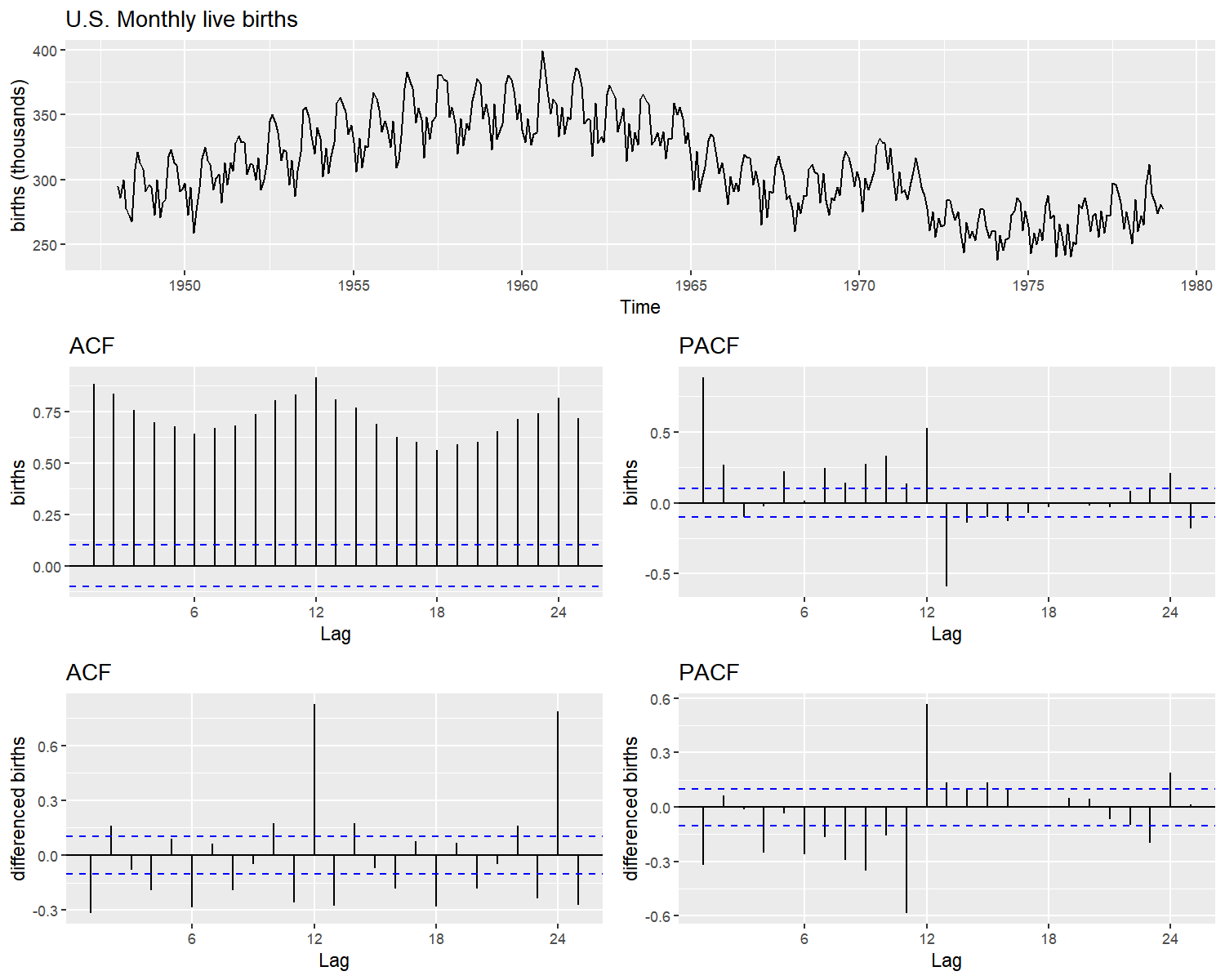
Figure 1: Monthly live birth U.S.A

For start, a seasonal ARIMA model could give a good fit to the data. Following Tsay (2010) recommendations for order selection using the auto-correlation functions, a p = 1, d = 1, q = 1 and for the seasonal part P = 1, D = 1, Q = 1. The model is defined in varstan as follows

R> model1 = Sarima(birth,order = c(1,1,1),seasonal = c(1,1,1)) R> model1

y   Sarima(1,1,1)(1,1,1)[12] 373 observations and 1 dimension Differences: 1 seasonal Differences: 1 Current observations: 360

Priors: Intercept: mu0   t (loc = 0 ,scl = 2.5 ,df = 6 )

Scale Parameter: sigma0   half_t (loc = 0 ,scl = 1 ,df = 7 )

ar[ 1 ]   normal (mu = 0 , sd = 0.5 ) ma[ 1 ]   normal (mu = 0 , sd = 0.5 )

Seasonal Parameters: sar[ 1 ]   normal (mu = 0 , sd = 0.5 ) sma[ 1 ]   normal (mu = 0 , sd = 0.5 ) NULL

The function Sarima generates a Seasonal ARIMA model ready to be fitted in Stan (Stan, Development. Team, 2017). As the model is printed, all the important information is shown: the model to be fit, the total observations of the data, the seasonal period, the current observations that can be used after differences, and a list of priors for all the model’s parameters. Using the information provided by the acf-plot in Figure 1 (middle right), the partial auto-correlations are not that strong, and a normal distribution for the auto-regressive coefficient (ar[1]) could explore values close to 1 or -1, causing the prior to be too informative. Instead beta distribution in $[-1,1]$ centered at zero, could be a more proper prior. With the functions set_prior() and get_prior() any change is automatically updated and checked.

R> model1 = set_prior(model = model1,dist = beta(2,2),par = "ar") R> get_prior(model = model1,par = "ar")

ar[ 1 ]   beta (form1 = 2 , form2 = 2 )

Now that the model and priors are defined, what follows is to fit the model using the varstan() function. One chain of 2,000 iterations and a warm-up of the first 1,000 chain’s values is simulated.

R> sfit1 = varstan(model = model1,chains = 1,iter = 2000,warmup = 1000) R> sfit1

y   Sarima(1,1,1)(1,1,1)[12] 373 observations and 1 dimension Differences: 1 seasonal Differences: 1 Current observations: 360

mean se 2.5mu0 0.0061 0.0020 0.0020 0.0101 3941.739 1.0028 sigma0 7.3612 0.0043 7.3528 7.3697 4001.665 1.0000 phi -0.2336 0.0014 -0.2362 -0.2309 3594.099 1.0007 theta 0.0692 0.0017 0.0658 0.0726 3808.853 1.0019 sphi -0.0351 0.0015 -0.0381 -0.0321 3376.811 1.0033 stheta 0.6188 0.0017 0.6153 0.6222 3427.074 1.0048 loglik -1232.2519 0.0325 -1232.3157 -1232.1882 3198.671 1.0033

Samples were drawn using sampling(NUTS). For each parameter, ess is the effective sample size, and Rhat is the potential scale reduction factor on split chains (at convergence, Rhat = 1).

All fitted models are varstan objects, these are S3 classes with the stanfit results provided by the rstan (Stan Development Team, 2020) package, and other useful elements that make the modeling process easier. After fitting the proposed model, a visual diagnostic of parameters, check residuals and fitted values using the plot methods. On figure 2 trace and posterior density plots are illustrated for all the model parameters.

R> plot(sfit1,type = "parameter")

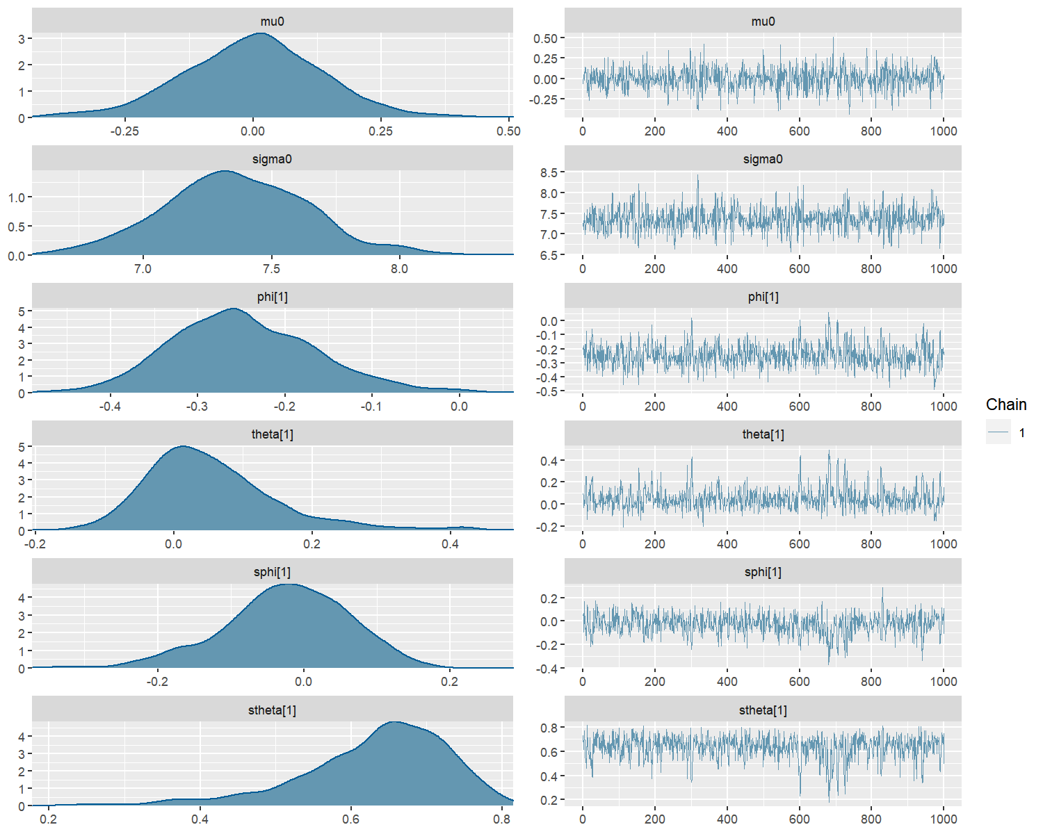
Figure 2: Trace and density plots for all the fitted parameters

In figure 2, all the chains appeared to be stationary, and the posteriors seems to have no multi-modal distributions. Indicating that all chains have mixed and converged. One useful way to assess models’ fit, is by the residuals ($e_{t}=Y_{t}-\widehat{Y}_{t}$). The package provides the posterior sample of every residual, but checking all of them is an exhausting task. An alternative, is checking the process generated by the residuals posterior estimate. A white noise behavior indicates a good model fit. The model’s residuals in figure 3, seems to follow a random noise, the auto-correlation in acf plots quickly falls to zero, indicating an acceptable model fit.

R> p1 = plot(sfit1,type = "residuals") R> p2 = plot(sfit1)

R> grid.arrange(p2,p1,ncol = 1)

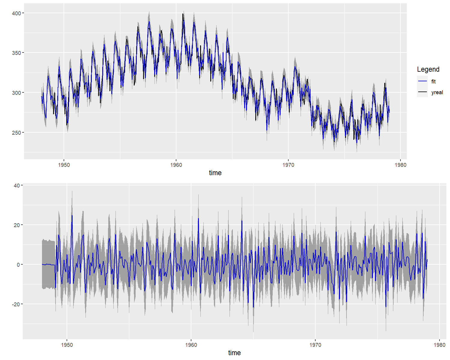
Figure 3: Posterior median residual plot

Because of the sinusoidal pattern that birth series (figure 1) presents, a dynamic Harmonic regression (A fourier transform with arima structure for errors) could also assess a good fit Kennedy (1992). To declare this model, varstan offers a similar declaration structure of forecast (Hyndman and Khandakar, 2008) package. A harmonic regression with 4 fourier terms and ARIMA(1,1,1) residuals is declared and fitted to the birth data.

R> model2 = Sarima(birth,order = c(1,1,1),xreg = fourier(birth,K = 2)) R> sfit2 = varstan(model = model2,chains = 1,iter = 2000,warmup = 1000) R> sfit2

y   Sarima(1,1,1).reg[4] 373 observations and 1 dimension Differences: 1, seasonal Differences: 0 Current observations: 372

mean se 2.5mu0 -0.0712 0.0068 -0.0846 -0.0578 939.6338 1.0032 sigma0 10.8085 0.0124 10.7841 10.8328 994.9722 1.0003 phi -0.2705 0.0019 -0.2742 -0.2668 1004.4136 1.0006 theta 0.6242 0.0015 0.6212 0.6272 921.6062 0.9992 breg.1 -21.6318 0.0407 -21.7116 -21.5520 965.9837 1.0006 breg.2 0.6619 0.0305 0.6021 0.7217 976.7075 1.0002 breg.3 4.7937 0.0207 4.7531 4.8344 1079.1161 1.0003 breg.4 -5.3570 0.0249 -5.4059 -5.3082 1099.4993 1.0005 loglik -1415.3887 0.0697 -1415.5252 -1415.2521 936.0271 1.0005

Samples were drawn using sampling(NUTS). For each parameter, ess is the effective sample size, and Rhat is the potential scale reduction factor on split chains (at convergence, Rhat = 1).

In this scenario both models suggest to be a good choice for birth series analysis. Even so, the harmonic regression fits more parameters. It is an obvious choice for birth’s sinusoidal behavior. As an example of model selection criteria, the bayes_factor in logarithmic scale, that compares the models’ marginal likelihoods is computed. Values above 6 (in logarithmic scale) provides good evidence for selecting the first model. And for birth data, the seasonal arima model (model1) is a better choice.

R> bayes_factor(x1 = sf1,x2 = sfit2,log = TRUE)

Iteration: 1 Iteration: 2 Iteration: 3 Iteration: 4 Iteration: 5 Iteration: 6 Iteration: 1 Iteration: 2 Iteration: 3 Iteration: 4 Iteration: 5 Iteration: 6 Estimated log Bayes factor in favor of model1 over model2: 199.13745

Now, a comparison of the selected model (model1 $\sim$ Sarima(1,1,1)(1,1,1)[12]) and the one given by the auto.sarima() function. For this purpose, a leave of one out cross validation loo() is used;, and both looic are compared with the loo_compare() function provided by the loo (Vehtari and Gabry, 2017) package.

R> sfit3 = auto.sarima(birth,chains = 1,iter = 4000) R> sfit3

y   Sarima(0,1,2)(1,1,1)[12] 373 observations and 1 dimension Differences: 1 seasonal Diferences: 1 Current observations: 360

mean se 2.5mu0 0.0080 0.0018 0.0045 0.0116 2050.372 0.9997 sigma0 7.3517 0.0060 7.3399 7.3634 1991.938 1.0008 theta.1 0.3642 0.0013 0.3616 0.3668 1978.174 1.0006 theta.2 0.1358 0.0011 0.1336 0.1379 2023.769 1.0004 sphi -0.2465 0.0016 -0.2496 -0.2433 2084.503 1.0005 stheta 0.3040 0.0017 0.3006 0.3073 2167.639 0.9995 loglik -1231.7452 0.0395 -1231.8225 -1231.6679 1789.987 1.0009

Samples were drawn using sampling(NUTS). For each parameter, ess is the effective sample size, and Rhat is the potential scale reduction factor on split chains (at convergence, Rhat = 1).

Different from model1, the selected one does not contemplate an auto-regressive component, and use 2 mean average components instead.Now what proceeds is to estimate the loo for both models:

R> loo1 = loo(sfit1) R> loo3 = loo(sfit3)

R> lc = loo::loo_compare(loo1,loo3) R> print(lc,simplify = FALSE)

elpd_diff se_diff elpd_loo se_elpd_loo p_loo se_p_loo looic se_looic model2 0.0 0.0 -1235.4 15.4 7.1 0.8 2470 30.8 model1 -0.8 5.8 -1236.2 15.6 7.8 0.9 2472 31.2

loo_compare() prints first the best model. In this example is the one provided by the auto.sarima() function, where its looic is 2 units below model1. This auto.sarima() function is useful as starting point. But the reader is encouraged to test more complex models and priors that adjust to the initial beliefs.

Conclusions

The paper gives a general overview of varstan package as a starting point of Bayesian time series analysis with structured models, and it offers a simple dynamic interface inspired in the classic functions provided by forecast, astsa, and var packages. The interface functions and prior flexibility that varstan offers, makes Bayesian analysis flexible as classic methods for structured linear time series models. The package’s goal is to provide a wide range of models with a prior selection flexibility. In a posterior version, non-linear models such as wackier GARCH variants, stochastic volatility, hidden Markov, state-space, and uni-variate Dynamic linear models will be included. Along with several improvements in the package’s functionality.

References

- Betancourt (2017) Betancourt M (2017). “A Conceptual Introduction to Hamiltonian Monte Carlo.” 1701.02434.
- Bierens (2006) Bierens HJ (2006). “Information Criteria and Model Selection.” Technical Report 3, Penssylvania State University, Pensylvania.
- Bollerslev (1986) Bollerslev T (1986). “Generalized autoregressive conditional heteroskedasticity.” Journal of Econometrics, 31(3), 307 – 327. ISSN 0304-4076. https://doi.org/10.1016/0304-4076(86)90063-1. URL http://www.sciencedirect.com/science/article/pii/0304407686900631.
- Box and Jenkins (1978) Box GEP, Jenkins G (1978). “Time series analysis: Forecasting and control. San Francisco: Holden-Day.” Biometrika, 65(2), 297–303. 10.1093/biomet/65.2.297. http://oup.prod.sis.lan/biomet/article-pdf/65/2/297/649058/65-2-297.pdf, URL https://doi.org/10.1093/biomet/65.2.297.
- Bürkner (2017) Bürkner PC (2017). “\pkgbrms: An \proglangR Package for Bayesian Multilevel Models Using \proglangStan.” Journal of Statistical Software, Articles, 80(1), 1–28. ISSN 1548-7660. 10.18637/jss.v080.i01. URL https://www.jstatsoft.org/v080/i01.
- Duane (1987) Duane S ea (1987). “Hybrid Monte Carlo.” Physics Letters B, 95(2), 216 – 222. ISSN 0370-2693. https://doi.org/10.1016/0370-2693(87)91197-X". URL http://www.sciencedirect.com/science/article/pii/037026938791197X.
- Engle (1982) Engle RF (1982). “Autoregressive Conditional Heteroscedasticity with Estimates of the Variance of United Kingdom Inflation.” Econometrica, 50(4), 987–1007. ISSN 00129682, 14680262. URL http://www.jstor.org/stable/1912773.
- Fonseca et al. (2019) Fonseca TCO, Cerqueira VS, Migon HS, Torres CAC (2019). “The effects of degrees of freedom estimation in the Asymmetric GARCH model with Student-t Innovations.” 1910.01398.
- Fonseca et al. (2008) Fonseca TCO, Ferreira MAR, Migon HS (2008). “Objective Bayesian analysis for the Student-t regression model.” Biometrika, 95(2), 325–333. ISSN 0006-3444. 10.1093/biomet/asn001. https://academic.oup.com/biomet/article-pdf/95/2/325/622763/asn001.pdf, URL https://doi.org/10.1093/biomet/asn001.
- Gabry and Mahr (2019) Gabry J, Mahr T (2019). “\pkgbayesplot: Plotting for Bayesian Models.” R package version 1.7.1, URL https://mc-stan.org/bayesplot.
- Gomez (1998) Gomez V (1998). “Automatic Model Identification in the Presence of Missing Observations and Outliers.”
- Goodrich et al. (2020) Goodrich B, Gabry J, Ali I, Brilleman S (2020). “\pkgrstanarm: Bayesian applied regression modeling via \proglangStan.” R package version 2.19.3, URL https://mc-stan.org/rstanarm.
- Gronau et al. (2017) Gronau QF, Sarafoglou A, Matzke D, Ly A, Boehm U, Marsman M, Leslie DS, Forster JJ, Wagenmakers EJ, Steingroever H (2017). “A Tutorial on Bridge Sampling.” 1703.05984.
- Gronau et al. (2020) Gronau QF, Singmann H, Wagenmakers EJ (2020). “\pkgbridgesampling: An \proglangR Package for Estimating Normalizing Constants.” Journal of Statistical Software, 92(10), 1–29. 10.18637/jss.v092.i10.
- Hannan and Rissanen (1982) Hannan EJ, Rissanen J (1982). “Recursive Estimation of Mixed Autoregressive-Moving Average Order.” Biometrika, 69(1), 81–94. ISSN 00063444. URL http://www.jstor.org/stable/2335856.
- Hoffman and Gelman (2014) Hoffman MD, Gelman A (2014). “The No-U-Turn Sampler: Adaptively Setting Path Lengths in Hamiltonian Monte Carlo.” Journal of Machine Learning Research, 15, 1593–1623. URL http://jmlr.org/papers/v15/hoffman14a.html.
- Hyndman et al. (2020) Hyndman R, Athanasopoulos G, Bergmeir C, Caceres G, Chhay L, O’Hara-Wild M, Petropoulos F, Razbash S, Wang E, Yasmeen F (2020). \pkgforecast: Forecasting functions for time series and linear models. R package version 8.12, URL http://pkg.robjhyndman.com/forecast.
- Hyndman and Khandakar (2008) Hyndman R, Khandakar Y (2008). “Automatic Time Series Forecasting: The \pkgforecast Package for \proglangR.” Journal of Statistical Software, Articles, 27(3), 1–22. ISSN 1548-7660. 10.18637/jss.v027.i03. URL https://www.jstatsoft.org/v027/i03.
- Kass and Raftery (1995) Kass RE, Raftery AE (1995). “Bayes Factors.” Journal of the American Statistical Association, 90(430), 773–795. ISSN 01621459. URL http://www.jstor.org/stable/2291091.
- Kennedy (1992) Kennedy P (1992). “Forecasting with dynamic regression models: Alan Pankratz, 1991, (John Wiley and Sons, New York), ISBN 0-471-61528-5, [UK pound]47.50.” International Journal of Forecasting, 8(4), 647–648. URL https://EconPapers.repec.org/RePEc:eee:intfor:v:8:y:1992:i:4:p:647-648.
- Lewandowski et al. (2009) Lewandowski D, Kurowicka D, Joe H (2009). “Generating random correlation matrices based on vines and extended onion method.” Journal of Multivariate Analysis, 100(9), 1989 – 2001. ISSN 0047-259X. https://doi.org/10.1016/j.jmva.2009.04.008. URL http://www.sciencedirect.com/science/article/pii/S0047259X09000876.
- Migon et al. (2014) Migon H, Gamerman D, Louzada F (2014). Statistical inference. An integrated approach. Chapman and Hall CRC Texts in Statistical Science. ISBN 9781439878804.
- Natarajan and Kass (2000) Natarajan R, Kass RE (2000). “Reference Bayesian Methods for Generalized Linear Mixed Models.” Journal of the American Statistical Association, 95(449), 227–237. 10.1080/01621459.2000.10473916. https://www.tandfonline.com/doi/pdf/10.1080/01621459.2000.10473916, URL https://www.tandfonline.com/doi/abs/10.1080/01621459.2000.10473916.
- \proglangR Core Team (2017) \proglangR Core Team (2017). \proglangR: A Language and Environment for Statistical Computing. \proglangR Foundation for Statistical Computing, Vienna, Austria. URL https://www.R-project.org/.
- Shumway and Stoffer (2010) Shumway R, Stoffer D (2010). Time Series Analysis and Its Applications: With R Examples. Springer Texts in Statistics. Springer New York. ISBN 9781441978646. URL https://books.google.es/books?id=dbS5IQ8P5gYC.
- Spiegelhalter et al. (2002) Spiegelhalter DJ, Best NG, Carlin BP, Van Der Linde A (2002). “Bayesian measures of model complexity and fit.” Journal of the Royal Statistical Society: Series B (Statistical Methodology), 64(4), 583–639. 10.1111/1467-9868.00353. https://rss.onlinelibrary.wiley.com/doi/pdf/10.1111/1467-9868.00353, URL https://rss.onlinelibrary.wiley.com/doi/abs/10.1111/1467-9868.00353.
- Stan, Development. Team (2017) Stan, Development Team (2017). “\proglangStan: A \proglangC++ Library for Probability and Sampling, Version 2.16.0.” URL http://mc-stan.org/.
- Stan Development Team (2020) Stan Development Team (2020). “\pkgRStan: the \proglangR interface to \proglangStan.” R package version 2.19.3, URL http://mc-stan.org/.
- Stoffer (2019) Stoffer D (2019). “\pkgastsa: Applied Statistical Time Series Analysis.” R package version 1.9, URL https://CRAN.R-project.org/package=astsa.
- Tsay (2010) Tsay RS (2010). Analysis of Financial Time Series. Second edi edition. Wiley-Interscience, Chicago. ISBN 978-0470414354. 10.1002/0471264105. arXiv:1011.1669v3.
- Vehtari et al. (2016) Vehtari A, Gelman A, Gabry J (2016). “Practical Bayesian model evaluation using leave-one-out cross-validation and WAIC.” Statistics and Computing, 27(5), 1413–1432. ISSN 1573-1375. 10.1007/s11222-016-9696-4. URL http://dx.doi.org/10.1007/s11222-016-9696-4.
- Vehtari and Gabry (2017) Vehtari A Gelman A, Gabry J (2017). “\pkgloo: Efficient Leave-One-Out Cross-Validation and WAIC for Bayesian Models. \proglangR Package.” URL https://github.com/jgabry/loo.
- Watanabe (2010) Watanabe S (2010). “Asymptotic Equivalence of Bayes Cross Validation and Widely Applicable Information Criterion in Singular Learning Theory.” Journal of Machine Learning Research, 11. URL http://www.jmlr.org/papers/volume11/watanabe10a/watanabe10a.pdf.
- Wuertz et al. (2020) Wuertz D, Setz T, Chalabi Y, Boudt C, Chausse P, Miklovac M (2020). \pkgfGarch: Rmetrics - Autoregressive Conditional Heteroskedastic Modelling. \proglangR package version 3042.83.2, URL https://CRAN.R-project.org/package=fGarch.