Sound Context Classification Basing on Join Learning Model and Multi-Spectrogram Features

Abstract

In this paper, we present a deep learning framework applied for Acoustic Scene Classification (ASC), the task of classifying scene contexts from environmental input sounds. An ASC system generally comprises of two main steps, referred to as front-end feature extraction and back-end classification. In the first step, an extractor is used to extract low-level features from raw audio signals. Next, the discriminative features extracted are fed into and classified by a classifier,reporting accuracy results. Aim to develop a robust framework applied for ASC, we address exited issues of both the front-end and back-end components in an ASC system, thus present three main contributions: Firstly, we carry out a comprehensive analysis of spectrogram representation extracted from sound scene input, thus propose the best multi-spectrogram combinations. In terms of back-end classification, we propose a novel join learning architecture using parallel convolutional recurrent networks, which is effective to learn spatial features and temporal sequences of spectrogram input. Finally, good experimental results obtained over benchmark datasets of IEEE AASP Challenge on Detection and Classification of Acoustic Scenes and Events (DCASE) 2016 Task 1, 2017 Task 1, 2018 Task 1A & 1B, LITIS Rouen prove our proposed framework general and robust for ASC task.

I Introduction

Acoustic Scene Classification (ASC), which aims to identify a sound scene context, vitally contributes to a variety of real-life applications ranging from security [1], surveillance [2] and context-aware consumer services [3, 4, 5]. Although ASC research is very close to Automatic Speech Recognition (ASR) and Speaker Recognition System (SRS) due to exploring audio signals, ASC currently presents various and different challenges. Firstly, there are a wide range of acoustic events in real-world environments, and these occur in different ways. Some sound events constitute natural auditory scenes that presents an acoustic mixture signal. For instance, bird sounds and the sounds of leaves, grass, or trees blowing in the wind clearly indicate certain context like in a park or on a field. However, it is more difficult to handle some sound events that are not context specific such as engine, or talking. This kind of context causes a confusion for even human (only listening) to recognize exactly in a street, on a transportation such as car, bus or tube or in a station. Indeed, experimental results in  [6] indicates that a proposed ASC system configured by Mel Frequency Cepstral Coefficients (MFCCs)-Hidden Markov Model (HMM) significantly outperformed human ability for recognizing everyday acoustic. Secondly, if sound events are considered as signal that mixed in diverse scenes as noise, there are different levels of signal-to-noise ratio (SNR) due to environmental conditions, distance of recording devices and so on. Moreover, these sounds exist across a wide range of frequency bands. Some occupy narrow frequency bands, while some spread over wide bands, and many sounds have frequency bands that overlap each other. Finally, natural sounds in ASC research do not follow any structure, unlike a speech signal.

To deal with these challenges, the state-of-the-art systems tend to make use of multi-input features. In particular, systems approaching frame-based features make effort to combine frequency and temporal features to maximize the chance of correct feature representation. For instance, MFCCs [7], one of most used frquency features, is combined with a wide range of temporal features such as loudness, average short-time energy, sub-band energy, zero-crossing rate, spectral flux, or spectral centroid in [8, 9, 10]. Similarly, an effective combination of MFCCs with a variety of features such as perceptual linear prediction (PLP) coefficients, power nomalised cepstral coefficients (PNCC), robust compressive gamma-chirp filter-bank cepstral coefficients (RCGCC) or subspace projection cepstral coefficients (SPPCC) was proposed in [11] that helps to achieve the top-three system in DCASE 2016 challenge. As usual, ASC systems approaching frame-based feature representation use traditional machine learning models for back-end classification, such as Hidden Markov Model (HMM) [6], Support Vector Machine (SVM) [12, 13], and Gaussian Mixture Model (GMM) [14].

Inspire that frame-based representation may not capture enough information, two-dimensional spectrograms as a more effective way for low-level feature representation have been exploited by the state-of-the-art ASC systems. In particular, spectrograms such as short term Fourier transform (STFT) [7], log-Mel [15, 16], MFCC [17], constant-Q transform (CQT) [18], and Gammatone spectrograms (GAM) [19, 20] are the most frequent low-level feature used. To further enrich input features, multiple spectrograms are widely approached. For instances, log-Mel is combined with a different types of spectrograms such as Mel-based nearest neighbour filter (NNF) spectrogram [21, 22], CQT [23], or two spectrograms such as MFCC and GAM in [19, 24]. Furthermore, the idea of generating multi-spectrogram input is also based on combinations of information from channels of recording devices. This idea has been proved its efficiency when Yuma et al. [25] did experiments to explore the average and difference of two channels, separated harmonic and percussive spectrograms from each channel, consequently achieved the top-one score in DCASE 2018 Task 1A challenge. Approach both frame-based and spectrogram representation, combined features such as MFCC+i-Vector or log-Mel+x-Vector were proposed in [26] and [23], respectively. To explore two-dimensional spectrogram representation, ASC systems usually deploy complicated classification models, mainly coming from deep learning techniques. For examples, Yang et al. [27] proposed a complicated CNN-based architecture called the Xception network. This is inspired by the fact that a deep learning network trained by a wide range of feature scales and over separated channels can result in a very powerful model. Besides, Truc et al. [21] applied a parallel CNNs to learn from two types of spectrogram (log-Mel and NNF). Next, the two outputs of the CNNs are concatenated to generate high-performed features that were thus explored by an DNN and achieve the highest accuracy rate in DCASE 2018 Task 1B challenge. Approach Recurrent Neural Network (RNN) based architecture, Zang et al. [28, 29, 30] provided a deep analysis of the application of Long Short-Term Memory (LSTM) for ASC. Other examples prove effective in exploiting RNN-based networks for ASC were published by Huy et al. [20, 31, 32]. Instead of using LSTM, Huy et al. proposed using Gate Recurrent Unit (GRU-based) based architecture [31]. Then they further improved the model by applying an attention scheme [20] or combining with a CNN-based architecture [32]. Compare to frame-based approach, ASC systems using spectrogram representation outperform and show more robust [19, 31, 32].

As the analysis of the-state-of-the-art ASC systems, we adopt the second trend that uses spectrogram representation for low-level feature input and explore deep learning model architecture for classification. In particular, we mainly contribute:

• Although spectrogram-based ASC systems explore multi-spectrogram input features to deal with ASC challenges, none of research has analysed and indicated the most effective combination of spectrograms. In this paper, we, therefore, provide a comprehensive analysis on spectrograms by conducting experiments on five common types of spectrograms, comprising of Short-time Fourier Transform (STFT), log-Mel, Mel Frequency Ceptral Coefficient (MFCC), Constant Q Transform (CQT), and Gammatone filter (GAM). To do this, we firstly introduce a C-DNN-based deep learning model, likely VGG-9 [33]. Consequently, we evaluate individual spectrograms on C-DNN network proposed, thus indicate the most effective combination of spectrograms due to late fusion of individual spectrogram accuracy.

• Next, we improve the C-DNN model by adding a parallel C-RNN based architecture to efficiently learn the structure of temporal sequences of spectrograms. By using a parallel CNN and C-RNN networks, we create a join learning architecture that is very useful to deploy the two-dimensional spectrogram input.

• To evaluate ASC systems, researches normally did experiments on one dataset [9, 11] . Some proposed to evaluate on two datasets [34, 15]. This may not conclude ASC systems proposed general or powerful. We, therefore, conduct extensive experiments, evaluating our proposed systems over five ASC datasets of DCASE 2016 Task 1, DCASE 2017 Task 1, DCASE 2018 Task 1A & 1B, and Litis Rouen published recently. Good results obtained from experiments on various datasets showing different category number, recording time, and wide range of real-life environments strongly prove the proposed system general and robust.

II Dataset and Setting

Our experiments are conducted over a variety of published ASC datasets, comprising of LITIS Rouen [35] and IEEE AASP Challenge on Detection and Classification of Acoustic Scenes and Events (DCASE) 2016 Task 1 [36] , 2017 Task 1  [17] , 2018 Task 1A & 1B [37].

LITIS Rouen dataset was recorded at a sample rate of 22050 Hz with 3026 segments, each presents 30-s duration. This dataset contains totally 25.51 recording hours for 19 urban scene categories, showing unbalanced data. Following the mandated settings, the dataset is separated and organised for 20-fold cross validation, reporting the final classification accuracy by averaging over the 20 testing folds.

DCASE 2016 Task 1 and DCASE 2017 Task 1 similarly present 15 categories and were recorded at 44.1 kHz. While each segment in DCASE 2016 is 30 s, 10-s duration is presented in DCASE 2017. Noticeably, DCASE 2017 reuses all DCASE 2016 and adds new data recorded. Obey the recommended setting, we train our proposed system on development set (Dev.) and evaluate on the evaluation set (Eva.). As regards DCASE 2018 Task 1A, it was recorded at 44.8 kHz, spanning 10 categories and used one recording device namely A. DCASE 2018 Task 1B reuses all data from DCASE 2018 Task 1A, and adds more data recorded by two different devices, namely B and C. Noticeably, the total recording time conducted on device B and C are much less than device A (denoted as DCASE 2018 Task 1A), reporting totally 4 hours on B&C compared to 24 hours in device A. As a result, DCASE 2018 Task 1B dataset involves issues of mismatched recording devices and unbalanced data in terms of recording devices. Therefore, DCASE 2018 Task 1B challenge only compare systems’ results on device B&C with less recording time. As DCASE 2018 Task 1A and 1B have not released labels of evaluation set, we separate development set into two sub-sets, namely Training and Test sets for training and testing processes respectively. While DCASE 2016 Task 1 and DCASE 2017 Task 1 are balanced, little unbalanced data is shown in DCASE 2018 Task 1A and 1B.

III High-level architecture

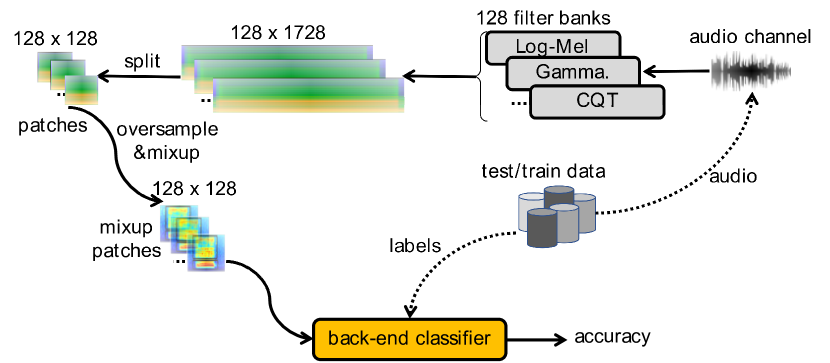
Figure 1: High-level architecture of our ASC system.

Our proposed deep learning framework applied for ASC, in general, is described in Figure 1. As Figure 1 shown, the framework is separated into low-level feature extraction (the upper part) and back-end classification (the lower part). In particular, the draw audio from the Channel 1 is firstly transformed into spectrogram representation, using 128 filter banks. The entire spectrogram is thus split into non-overlapped image patches of $128\times 128$. To deal with unbalanced data issue, we apply two data augmentation techniques on the image patches. Firstly, we randomly oversample image patches which belong in categories with less audio segments. Next, the mixup data augmentation [38] is applied, thus generate new image patches. Let’s consider two original image patches as $\mathbf{X_{1}}$, $\mathbf{X_{2}}$ and expected labels as $\mathbf{y_{1}}$, $\mathbf{y_{2}}$, new image patches are generated as below equations:

$$\mathbf{X_{mp1}}=\mathbf{X_{1}}*\gamma+\mathbf{X_{2}}*(1-\gamma)$$ (1)

$$\mathbf{X_{mp2}}=\mathbf{X_{1}}*(1-\gamma)+\mathbf{X_{2}}*\gamma$$ (2)

$$\mathbf{y_{mp1}}=\mathbf{y_{1}}*\gamma+\mathbf{y_{2}}*(1-\gamma)$$ (3)

$$\mathbf{y_{mp2}}=\mathbf{y_{1}}*(1-\gamma)+\mathbf{y_{2}}*\gamma$$ (4)

where $\gamma$ is random coefficient from both unit and beta distribution, $\mathbf{X_{mp1}}$, $\mathbf{X_{mp2}}$ and $\mathbf{y_{mp1}}$, $\mathbf{y_{mp2}}$ are new image patches and labels generated, respectively. Eventually, the mixup patches are fed into a back-end classifier, report the classification accuracy.

IV An analysis of spectrogram features

By using the high-level architecture mentioned above, we evaluate five individual spectrograms (STFT, log-Mel, MFCC, GAM, and CQT), thus indicate which kind of spectrograms and their combinations is the most influencing on our system’s performance. To evaluate the individual spectrograms, we firstly proposed a C-DNN based network referred to as the back-end classifier. Next, we create five systems, each reuse the high-level framework architecture mentioned with one type of spectrogram and C-DNN architecture for classification. Noting that we use same setting with window size=1290, hop size=256, frequency minimum$f_{min}$=10 Hz, and filter bank number=128 to generate same-size spectrograms. The results of five systems over DCASE 2018 Task 1B dataset are analysed and compare to the DCASE baseline. Inspire that each spectrogram contain discriminative and complementary features, we fuse the individual systems’ accuracy results, thus indicate which combination of spectrograms is effective to improve the performance.

IV-A C-DNN architecture proposed for back-end classification

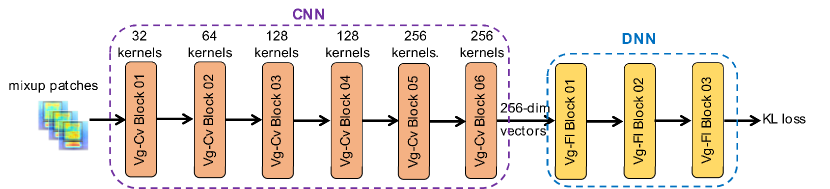
Figure 2: Block-level architecture of C-DNN network.

TABLE I: Network layers used in C-DNN architecture.

	Blocks	Layers	Outptut shape
	Input		$128{\times}128{\times}1$
	Vg-Cv Block 01	Bn - Cv [$9\times 9$] - ReLu - Bn - Ap [$2\times 2$] - Dr (10%)	$64{\times}64{\times}32$
	Vg-Cv Block 02	Cv [$7\times 7$] - ReLu - Bn - Ap [$2\times 2$] - Dr (15%)	$32{\times}32{\times}64$
CNN	Vg-Cv Block 03	Cv [$5\times 5$] - ReLu - Bn - Dr (20%)	$32{\times}32{\times}128$
Architecture	Vg-Cv Block 04	Cv [$5\times 5$] - ReLu - Bn - Ap [$2\times 2$] - Dr (20%)	$16{\times}16{\times}128$
	Vg-Cv Block 05	Cv [$3\times 3$] - ReLu - Bn - Dr (25%)	$16{\times}16{\times}256$
	Vg-Cv Block 06	Cv [$3\times 3$] - ReLu - Bn - Gap - Dr (25%)	$256$
	Vg-Fl Block 01	Fl - ReLu - Dr (30%)	$512$
DNN	Vg-Fl Block 02	Fl - ReLu - Dr (30%)	$1024$
Architecture	Vg-Fl Block 03	Fl - Softmax	10

In order to evaluate individual and multiple spectrograms, we proposed a C-DNN network architecture as described in Figure 2 and Table I. As Figure 2 shown, C-DNN architecture comprises of CNN and DNN parts in order. CNN part is described by 6 Vg-Cv blocks, performed by Batchnorm (Bn), Convolutional (Cv[kernel size]), Rectified linear unit (ReLu), Dropout (Dr(Percentage dropped)), Average Pooling (Ap), Global Average Pooling (Gap) layers as showed in the top of Table I. Meanwhile, DNN part in Figure 2 is configured by three Vg-Fl blocks with Fully-connect (Fl), ReLu, Dropout (Dr(Percentage dropped)), and Softmax layers, as described in the bottom of Table I. It can be seen that CNN part helps to map input image patches to condensed and discriminative vectors, referred to as high-level features. Each high-level feature vector presents 256 dimensions due to the number of kernels used in the final convolutional layer in Vg-Cv block 06. Next, DNN part explores the high-level features, thus classifies into 10 categories (the category number in DCASE 2018 Task 1B dataset evaluated) and reports the classification accuracy.

IV-B Spectrogram representation and their combinations proposed

To propose spectrogram combinations, formulas of individual spectrograms are firstly presented below:

Short-Time Fourier Transform (STFT): The first STFT spectrogram evaluated applies Fourier Transform to extract Frequency content of local section of input signal over short time duration. Let consider $\mathbf{s}$($n$) as digital audio signal with length of $N$ , a pixel value at central frequency $f$ and time frame $t$ of STFT spectrogram $\mathbf{STFT}[F,T]$ is computed as:

$$\mathbf{STFT}[f,t]=\sum_{n=0}^{N-1}\mathbf{s}[n].\mathbf{w}[t]e^{-j2{\pi}fn}$$ (5)

where $\mathbf{w}$[$t$] is a window function, typically Hamming. While time resolution ($T$) of STFT spectrogram is set by window side and hope size, the frequency resolution ($F$) equals to the number of central frequencies set to 2048. The frequency resolution, eventually, re-scales into 128 that is same as other spectrograms.

log-Mel: To generate log-Mel spectrogram, draw audio signal is firstly transformed into STFT spectrogram recently mentioned. Next, a Mel filter bank, which simulates the overall frequency selectivity of the human auditory system using the frequency warping $F_{mel}=2595.log(1+{F}/{700})$ [7], is applied to generate a Mel spectrogram $\mathbf{MEL}[F_{mel},T]$ (noting that frequency resolution ($F_{mel}$) is the Mel filter number set to 128). Eventually, logarithmic scaling is applied to obtain the log-Mel spectrogram. Let consider $\mathbf{COE}[F_{mel},F]$ as matrix storing coefficients of Mel filters, log-Mel spectrogram likely a matrix is computed by:

$$\mathbf{log{-}Mel}[F_{mel},T] {}={} log\mathbf{COE}[F_{mel},F]$$ (6)

$$.\mathbf{STFT}[F,T]$$

Mel Frequency Cepstral Coefficient (MFCC): From log-Mel spectrogram, Discrete Cosine Transform (DCT) is used to extract a sequence of uncorrelated coefficients crossing frequency dimension, reducing log-Mel frequency resolution into smaller space. A pixel value $\mathbf{DCT}[f_{dct},t_{dct}]$ of DCT matrix $\mathbf{DCT}[F_{dct},T_{dct}]$, where $F_{dct}$ and $T_{dct}$ are frequency and time resolutions, is computed by:

$$\mathbf{DCT}[f_{dct},t_{dct}] {}={} \left(\frac{2}{F_{mel}}\right)^{\frac{1}{2}}.\left(\frac{2}{T}\right)^{\frac{1}{2}}.\sum_{f_{mel}=0}^{F_{mel}-1}.\sum_{t=0}^{T-1}$$ (7)

$$\Lambda(f_{mel}).cos\left[\frac{{\pi}f_{dct}}{F_{mel}}(2f_{mel}+1)\right]$$

$$.\Lambda(t).cos\left[\frac{{\pi}t_{dct}}{T}(2t+1)\right]$$

$$.\mathbf{log{-}Mel}[f_{mel},t]$$

where

$$\Lambda(x)=\begin{cases}\frac{1}{\sqrt{2}}&\text{if }x=0\\ 1&\text{otherwise}\end{cases}$$ (8)

$T$ and $F_{mel}$ are time and frequency resolution of log-Mel spectrogram.

Next, delta coefficients per time frame showing difference of DCT coefficients over time are computed, shown in Equation. (9).

$$\mathbf{DELTA}[F_{dct},t] {}={} \frac{1}{2}(\mathbf{DCT}[F_{dct},t-1]$$ (9)

$$-\mathbf{DCT}[F_{dct},t+1])\$$

Eventually, $\mathbf{DELTA}[F_{dct},T_{dct}]$ is concatenated with DCT spectrogram $\mathbf{DCT}[F_{dct},T_{dct}]$ across frequency dimension to generate MFCC spectrogram as expression $\mathbf{MFCC}[F_{mfcc},T_{dct}]$ (noting that MFCC frequency resolution ($F_{mfcc}$) doubles frequency resolution of DCT ($F_{dct}$) and equals to 128, and $T_{dct}$ is set to equal to $T$ resolution of log-Mel spectrogram).

Constant Q transform (CQT): This spectrogram applies a bank of filters corresponding to tonal spacing, where each filter is equivalent to a subdivision of an octave, with central frequencies given by:

$$f_{k}=(2^{\frac{1}{b}})^{k}.f_{min}~{}~{}~{}for~{}~{}1\leq k\leq K$$ (10)

where $f_{k}$ denotes the frequency of $k$th spectral component, $f_{min}$ is minimum frequency set to 10 Hz, $b$ is the number of filters per octave as 24, and $K$ is frequency resolution of CQT, which is 128. As the name suggest, the $Q$ value, is the ratio of central frequency to bandwidth, is constant computed as:

$$Q=\frac{f_{k}}{\Delta f_{k}}=\frac{f_{k}}{f_{k+1}-f_{k}}=\left(2^{\frac{1}{b}}-1\right)^{-1}$$ (11)

Like STFT, CQT spectrogram is extracted using Fourier-based transformation, described as Equation (12) :

$$\mathbf{CQT}[f_{k},t]=\frac{1}{N(k)}.\sum_{n=0}^{N(k)-1}\mathbf{s}[n].\mathbf{w}[k,n-t].e^{-i2\pi\frac{nQ}{N(k)}}$$ (12)

where:

$$N(k)=Q.\frac{f{s}}{f_{k}}$$ (13)

$$\mathbf{w}[k,n]=\alpha+(1-\alpha).cos\frac{2{\pi}n}{N(k)-1}$$ (14)

$f{s}$ is sample rate of digital input signal $\mathbf{s}[n]$, $\mathbf{w}[k,n]$ is window function with $\alpha$ set to 0.54. To generate STFT, log-Mel, MFCC, and CQT, we use a popular audio toolbox, namely Librosa [39].

Gammatone (GAM): Gammatone filters are designed to model the frequency-selective cochlea activation response of the human inner ear [40], in which filter output simulates the frequency response of the basilar membrane. The impulse response is given by:

$$g(t)=t^{P-1}e^{-2lt\pi}cos(2ft\pi+\theta)$$ (15)

where $t$ is time, $P$ is the filter order, $\theta$ is the phase of the carrier, $l$ is filter bandwidth, and $f$ is central frequency. The filter bank was then formulated as ERB scale [41] as:

$$ERB=24.7(4.37.10^{-3}f+1)$$ (16)

To quickly generate Gamma spectrogram, we apply a toolbox developed by Ellis et al. [42], namely Gammatone-like spectrogram. Firstly, audio signal is transformed into STFT spectra recently mentioned above. Next, gammatone weighting $\mathbf{COE}[F_{gam},F]$ is applied on STFT to obtain the Gamma spectrogram.

$$\mathbf{GAM}[F_{gam},T]=\mathbf{COE}[F_{gam},F].\mathbf{STFT}[F,T]$$ (17)

where $F_{gam}$ resolution of GAM spectrogram is Gammatone filter number of 128.

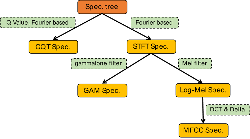
Figure 3: Constructed spectrogram tree basing on difference of central frequencies and auditory models applied.

TABLE II: Spectrogram combinations proposed.

Group of	Combinations of
Two spectrograms	CQT+STFT, CQT+GAM,
	CQT+log-Mel, CQT+MFCC
Three spectrograms	CQT+log-Mel+GAM,
	CQT+GAM+MFCC
Four spectrograms	CQT+GAM+STFT+MFCC,
	CQT+GAM+STFT+log-Mel
Five spectrograms	CQT+log-Mel+GAM+STFT+MFCC

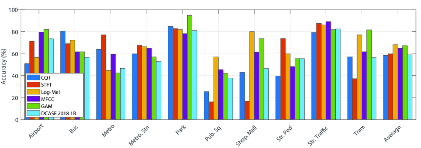
Figure 4: Category-wise performance comparison among spectrograms on device A - DCASE 2018 Task 1B.

As spectrogram formulas described, we construct a spectrogram tree as shown in Figure 3. Firstly, although both of CQT and STFT spectrograms are built on Fourier Transform theory, they extract different central frequencies. From the root tree, we therefore separate into two main branches of CQT and STFT. From the branch of STFT spectrogram, we continuously divide into log-Mel and GAM spectrograms due to applying different Mel and Gammatone filters, respectively. Eventually, MFCC is an extended branch from log-Mel due to extracting DCT and Delta from this spectrogram. It can be seen that five spectrograms proposed either extract different central frequencies or apply different auditory models. Therefore, each spectrogram may contain its own distinct and complimentary information. This inspires us to conduct experiments to indicate how individual spectrograms and their combinations affect to an ASC system’s performance. Based on the tree shown in Figure 3, we propose a variety of combinations as denoted in Table II. In particular, two-spectrogram combinations are inspired from two main branches from the root tree, each extracts specific central frequencies. Thus, we create groups of CQT+STFT, CQT+GAM, CQT+log-Mel, and CQT+MFCC. There are two third-spectrogram groups of CQT+GAM+log-Mel and CQT+GAM+MFCC evaluated, which inspires from exploring different central frequencies between CQT & STFT branches and different auditory models used among MFCC, log-Mel, and GAM. Inspire that applying auditory models on STFT may destroy discriminative features on this spectrogram and two spectrograms of MFCC, log-Mel may contain very similar features due to coming from same Mel filter banks, we propose two four-spectrogram combinations, which are CQT+GAM+STFT+MFCC and CQT+GAM+STFT+log-Mel. Eventually, the combination of all five spectrograms is also evaluated.

IV-C Late fusion strategy to evaluate spectrogram combinations

As the back-end classification works on smaller patches, the posterior probability of an entire spectrogram is computed by averaging of all patches’ posterior probabilities. Let us consider $\mathbf{P^{n}}=(\mathbf{p_{1}^{n},p_{2}^{n},...,p_{C}^{n}})$, with $C$ being the category number and the $n^{th}$ out of $N$ patches fed into learning model, as the probability of a test sound instance, then the mean classification probability is denoted as $\mathbf{\bar{p}}=(\bar{p}_{1},\bar{p}_{2},...,\bar{p}_{C})$ where,

$$\bar{p}_{c}=\frac{1}{N}\sum_{n=1}^{N}p_{c}^{n}~{}~{}~{}for~{}~{}1\leq n\leq N$$ (18)

and the predicted label $\hat{y}$ for an individual spectrogram evaluated is determined using:

$$\hat{y}=argmax(\bar{p}_{1},\bar{p}_{2},...,\bar{p}_{C})$$ (19)

To evaluate the combinations of spectrograms, we proposed a late fusion scheme, namely Mean fusion. In particular, we conduct experiments over individual spectrograms, thus obtain posterior probability of each spectrogram as $\mathbf{\bar{p_{s}}}=(\bar{p}_{s1},\bar{p}_{s2},...,\bar{p}_{sC})$ where $C$ is the category number and the $s^{th}$ out of $S$ spectrograms evaluated. Next, the posterior probability after late fusion $\mathbf{p_{f-mean}}=(p_{1},p_{2},...,p_{C})$ is obtained from by:

$$p_{c}=\frac{1}{S}\sum_{s=1}^{S}\bar{p}_{sc}~{}~{}~{}for~{}~{}1\leq s\leq S$$ (20)

Eventually, the predicted label $\hat{y}$ is determined by:

$$\hat{y}=argmax({p}_{1},{p}_{2},...,{p}_{C})$$ (21)

IV-D Hyperparameter setting and dataset used to evaluate

In this work, we adopt Tensorflow framework to build deep leaning models with learning rate of 0.0001, a batch size of 50, epoch number of 100, and Adam method [43] for learning rate optimization. As using mixup data augmentation, the labels are not one-hot format. Therefore, we use Kullback-Leibler (KL) divergence loss [44] instead of the standard cross-entropy loss as shown in Equation below:

$$Loss_{KL}(\theta)=\sum_{n=1}^{N}\mathbf{y}_{n}\log(\frac{\mathbf{y}_{n}}{\mathbf{\hat{y}}_{n}})+\frac{\lambda}{2}||\theta||_{2}^{2},$$ (22)

where $Loss_{KL}(\theta)$ is KL-loss function, $\theta$ describes the trainable parameters of the network trained, $\lambda$ denote the $\ell_{2}$-norm regularization coefficient experimentally set to 0.0001, $N$ is the batch size, $\mathbf{y_{c}}$ and $\mathbf{\hat{y}_{c}}$ are the ground-truth and the network recognized output, respectively. Noting that we use only DCASE 2018 Task 1B dataset to analyse individual spectrograms and their combinations proposed.

IV-E Performance comparison over spectrograms and their combinations

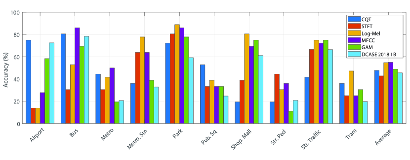
Figure 5: Category-wise performance comparison among spectrograms on device B&C - DCASE 2018 Task 1B.

At initial, we equally evaluate all of five individual spectrograms by feeding them into the C-DNN network, thus show category-wise performance comparison of device A and device B&C of DCASE 2018 Task 1B dataset. As obtained results on device A in Figure 4, log-Mel, GAM, and MFCC generally outperform STFT and CQT on most categories. As regards the average accuracy, log-Mel and GAM stand on the top, showing competitive results of 68.2% and 67.2%, respectively. Meanwhile, STFT and CQT show very low average scores compared with log-Mel and GAM, indicating a gap performance of nearly 10%. Noticeably, CQT spectrogram showed great performance in sound scenes belong to transportation such as Bus, Metro and Street Traffic.

Regarding performance on device B&C in Figure 5, obtained results show similar with top scores of log-Mel, GAM, and MFCC. Again, CQT spectrogram still shows good accuracy rate in related-transformation categories such as Bus, Metro and Tram.

In general, category-wise performance comparison of device A and device B&C indicate that spectrograms extracted from auditory models such as GAM, log-Mel and MFCC gain high performance. Compare these three spectrograms to the DCASE 2018 baseline as regards Task 1B challenge (only device B&C), they outperform the DCASE 2018 baseline over almost categories and show an improvement of 3.3%, 9.1%, and 9.4% respectively in terms of the average result.

Next, we conduct experiments on two-spectrogram combinations and present obtained results in Table III. As Table III shown, CQT+log-Mel achieves the greatest performance on both device A and B&C, improving by 4% and 6% respectively compared to only log-Mel (the top score of individual spectrogram). Compare CQT+log-Mel score to DCASE 2018 Task 1B baseline, it shows a significant improvement of 13.1% and 15.2% over device A and B&C, respectively.

TABLE III: Compare individual spectrograms and their combinations to DCASE 2018 Task 1B baseline with best results (%) in bold.

Spectrograms	A	B&C	A&B&C
DCASE baseline	58.9	45.6	52.2
Single spectrogram
MFCC	64.9	55.0	59.9
STFT	59.8	42.7	51.3
log-Mel	68.2	54.7	61.4
CQT	58.4	47.8	53.1
GAM	64.1	48.9	58.1
Two spectrograms
CQT+STFT	64.2	55.8	60.0
CQT+GAM	70.9	53.3	62.1
CQT+log-Mel	72.0	60.8	66.4
CQT+MFCC	69.8	58.9	64.4
Three spectrograms
CQT+GAM+log-Mel	74.1	62.5	68.3
CQT+GAM+MFCC	71.9	61.1	66.5
Four spectrograms
CQT+GAM+STFT+log-Mel	74.4	62.5	68.5
CQT+GAM+STFT+MFCC	72.7	60.3	66.5
All five spectrograms
CQT+GAM+STFT+log-Mel+MFCC	73.7	62.8	68.2

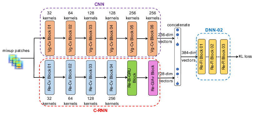
Figure 6: Joint learning network architecture.

TABLE IV: C-RNN network architecture.

Blocks	Layers	Output shape
	Input	$128{\times}128{\times}1$
Re-Cv Block 01	Bn - Cv [$4\times 1$] - ReLu - Bn - Ap [$2\times 1$] - Dr (10%)	$64{\times}128{\times}32$
Re-Cv Block 02	Cv [$4\times 1$] - ReLu - Bn - Ap [$2\times 1$] - Dr (15%)	$32{\times}128{\times}64$
Re-Cv Block 03	Cv [$4\times 1$] - ReLu - Bn - Ap [$2\times 1$] - Dr (20%)	$16{\times}128{\times}128$
Re-Cv Block 03	Cv [$4\times 1$] - ReLu - Bn - Ap [$16\times 1$] - Dr (20%)	$128{\times}256$
Re-Bi-GRU Block	Bi-GRU (128 hidden states, 30% dropout)	$128{\times}256$
Re-GlAv Block	Gap	$128$

As regards three-spectrogram combinations as shown in Table III, two groups of CQT+GAM+MFCC and CQT+log-Mel+GAM analysed show competitive results, reporting 71.9%, 61.1% and 74.1%, 62.5% for device A and B&C, respectively. It indicates that log-Mel and MFCC may contain very similar features.

The results on four-spectrogram combinations of CQT+GAM+STFT+log-Mel witness a minor increase of nearly 0.3% and 0.2% in terms of device A and overall respectively, compared to CQT+log-Mel+GAM, thank to the contribution of STFT. Meanwhile, adding STFT into CQT+GAM+MFCC only helps to improve the performance on device A a little, but makes a decrease of 0.8% on device B&C. As regards the result of all five spectrograms, it even has a downward trend in device A, leading to the a decrease of 0.7 %, compared to overall accuracy in the best four-spectrogram combination of CQT+GAM+STFT+log-Mel.

IV-F Discussion

Eventually, we summary all types of spectrogram combinations, and highlight which achieve the best scores on all three devices A&B&C. As results shown in Table III, there is a gradual increase in the accuracy rate when combination of spectrograms are applied. In particular, CQT+log-Mel achieves the best performance in two-spectrogram groups, with an increase of nearly 5% compared to the best single spectrogram log-Mel. By adding GAM into group of CQT+log-Mel, it helps to improve by 2% on average. However, a minor increase of 0.2% is observed in the performance of four-spectrogram combination CQT+GAM+STFT+log-Mel until there is no improvement from combination of all five spectrograms. It can be concluded that using multiple spectrograms is effective to improve the performance, thus far exceed the DCASE 2018 Task 1B baseline.

V Robust deep learning framework for ASC

V-A Join learning deep neural network architecture proposed.

As the analysis results on spectrogram, it can be seen that using multi-spectrogram input features is effective to improve the ASC system’s performance. To further enhance, we next make effort to improve the back-end classification, thus propose a join learning model, as described in Figure 6. As Figure 6 shown, we reuse the CNN part with six Vg-Cv blocks from the C-DNN architecture. These Convolutional blocks help to capture spatial features from spectrogram input, thus transform image patches into condensed and discriminative vectors with 256 dimension. Additionally, we add a parallel C-RNN architecture (the lower part of Figure 6) that is used to capture structures of temporal sequences from spectrogram input. As Table IV showing the C-RNN proposed, input patches of $128\times 128$ are fed into sub-blocks Cv, Bn, ReLu, Ap and Dr that are similar to those used in the CNN part. However, we adjust settings of these sub-blocks to allow the C-RNN network be able to learn time-sequential features. In particular, convolutional layers (Cv) with kernel size set to [$4\times 1$] are applied to learn the difference between frequency banks in each temporal frame. Next, average pooling layers (Ap [$2/16\times 1$]) is used to scale the frequency dimension of the spectrogram, but remain time resolution of 128. As a result, frequency dimension is scaled into 1, generating a sequence of 128-temporal frames after four Re-Cv blocks. Each temporal frame is represented by a 256-dimensional vector. Next the temporal sequence is fed into bi-GRU layer in Re-Bi-GRU Block which learns the temporal sequence structure from two directions. The output of Re-Bi-GRU Block is a matrix of $128\times 256$ with 128 temporal frames and 256 dimension each frame. Next, a Global Average Pooling layer in Re-GlAv block is applied on each temporal frame to get average results, generating a 128-dimensional vectors. Both output of C-RNN and CNN are thus concatenated, generate 384-dimensional vectors. Next, these vectors are fed into a DNN-02 architecture, as shown in Table V, configured by Fl, ReLu, Dr, and Softmax layers for classification. Noting that output layer number $C$ depends on specific ASC task due to various datasets evaluated.

TABLE V: DNN-02 network architecture.

Blocks	Layers	Output shape
	Input	$384$
Re-Fl Block 01	Fl - ReLu - Dr (30%)	$2048$
Re-Fl Block 02	Fl - ReLu - Dr (30%)	$1024$
Re-Fl Block 03	Fl - Softmax	$C$

V-B Hyperparameter setting for the framework proposed.

The join learning model proposed is built by Tensorflow framework and reused all hyper-parameter setting from C-DNN network experiments. To evaluate the effect of spectrograms, we conduct experiments on the best spectrogram combinations indicated in Table III in Section IV-E.

Additionally, we do further investigation of late fusion on accuracy. In particular, we compute more two fusion strategies, called Max and Prod fusions. Let us consider posterior probability of each spectrogram describes as $\mathbf{\bar{p_{s}}}=(\bar{p}_{s1},\bar{p}_{s2},...,\bar{p}_{sC})$ described in Equation (18), where $s$ is specific spectrogram and $C$ is the number of category classified. Next, the posterior probability of combination with Prod strategy $\mathbf{p_{f-prod}}=(p_{1},p_{2},...,p_{C})$ is obtained by,

$$p_{c}=\frac{1}{S}\prod_{s=1}^{S}\bar{p}_{sc}~{}~{}~{}for~{}~{}1\leq s\leq S$$ (23)

where $S$ is the number of spectrograms combined. The posterior probability of combination with MAX strategy $\mathbf{p_{f-max}}=(p_{1},p_{2},...,p_{C})$ is obtained by,

$$p_{c}=max(\bar{p}_{1c},\bar{p}_{2c},...,\bar{p}_{Sc})$$ (24)

Eventually, the predicted label $\hat{y}$ for either Max or Prod fusions is determined by Equation (21).

As regards ASC datasets evaluated, we conduct extensive experiments on five different datasets, comprising of Litis Rouen, DCASE 2016 Task 1A, DCASE 2017 Task 1A, and DCASE 2018 Task 1A and 1B. Thus, we compare our best results to the state-of-the-art systems.

V-C Performance comparison on DCASE 2018 Task 1B dataset

As results obtained in Table VI, adding the C-RNN architecture into C-DNN network to create the join learning model helps to improve the performance over both device A and B&C. Specially, the accuracy rate increases when more spectrograms are combined.

As regards late fusion methods suggested, Prod and Mean are very competitive and outperform Max fusion scheme in both C-DNN and join learning model proposed. Noticeably, join learning models with Prod fusion achieve the best scores for all kinds of spectrogram combinations in terms of B&C performance.

Compare to DCASE 2018 Task 1B baseline, join learning models proposed outperform DCASE baseline on both device A and B&C. In particular, the best score of 67.5% over devices B&C, which is obtained from combination of all spectrograms CQT+log-Mel+GAM+STFT+MFCC, significantly improves the DCASE baseline by 22%. It indicates that the strategy of multi-spectrogram input successfully solve the problem of mismatched devices raised in DCASE 2018 Task 1B challenge.

TABLE VI: Performance comparison (%) on DCASE 2018 Task 1B dataset with the highest scores in bold.

Architecture		Join Learning Model			C-DNN
Device A	Mean	Prod	Max	Mean	Prod	Max
CQT+log-Mel	72.4	72.1	70.9	72.0	73.0	70.1
CQT+log-Mel+GAM	74.9	74.5	73.4	74.1	74.7	72.3
CQT+log-Mel+GAM+STFT	76.2	76.5	73.6	74.4	74.9	71.5
CQT+log-Mel+GAM+STFT+MFCC	76.0	76.4	74.0	73.7	74.6	71.5
Devices B & C:	Mean	Prod	Max	Mean	Prod	Max
CQT+log-Mel	62.2	64.7	60.3	60.8	62.2	59.2
CQT+log-Mel+GAM	65.00	66.4	61.9	62.5	63.3	59.2
CQT+log-Mel+GAM+STFT	64.44	66.7	60.6	62.5	60.6	58.3
CQT+log-Mel+GAM+STFT+MFCC	65.3	67.5	64.7	62.8	61.9	58.1

TABLE VII: Comparison to state-of-the-art systems with best performance in bold (Upper part: top-ten DCASE challenges; Middle part: State-of-the-art papers; Low part: Our proposed systems using Prod late fusion strategy ).

D. 2018 Task 1B	Acc.	D. 2018 Task 1A	Acc.	D. 2017 Task 1	Acc.	D. 2016 Task 1	Acc.	LITIS Roune	Acc.
(Dev. set)	(%)	(Dev. set)	(%)	(Eva. set)	(%)	(Eva. set)	(%)	(20-fold Ave.)	(%)
Baseline [37]	45.6	Baseline [37]	59.7	Baseline [36]	74.8	Baseline [45]	77.2
Li [34]	51.7	Li [46]	72.9	Zhao [47]	70.0	Wei [48]	84.1	Bisot [49]	93.4
Tchorz [50]	53.9	Jung [26]	73.5	Jung [51]	70.6	Bae [52]	84.1	Ye [53]	96.0
Kong [54]	57.5	Wang [55]	73.6	Karol [56]	70.6	Kim [57]	85.4	Huy [24]	96.4
Wang [58]	57.5	Christian [59]	74.7	Ivan [60]	71.7	Takahasi [61]	85.6	Yin [62]	96.4
Waldekar [63]	57.8	Zhang [64]	75.3	Park [65]	72.6	Elizalde [66]	85.9	Huy [19]	96.6
Zhao [15]	63.3	Li [34]	76.1	Lehner [67]	73.8	Valenti [68]	86.2	Ye [69]	97.1
Truc [21]	63.6	Dang [70]	76.7	Hyder [71]	74.1	Marchi [9]	86.4	Huy [32]	97.8
		Octave [72]	78.4	Zhengh [73]	77.7	Park [11]	87.2	Zhang [30]	97.9
		Yang [27]	79.8	Han [74]	80.4	Bisot [75]	87.7	Zhang [28]	98.1
		Golubkov [76]	80.1	Mun [77]	83.3	Hamid [78]	89.7	Huy [31]	98.7
Zhao [15]	63.3	Bai [79]	66.1	Zhao [80]	64.0	Mun [81]	86.3
Truc [22]	64.7	Gao [82]	69.6	Yang [83]	69.3	Li [84]	88.1
Truc [85]	66.1	Zhao [15]	72.6	Waldekar [63]	69.9	Hyder [86]	88.5
Yang [87]	67.8	Phaye [16]	74.1	Wu [88]	75.4	Song [89]	89.5
		Heo [90]	77.4	Chen [91]	77.1	Yin [62]	91.0
log-Mel	58.6	log-Mel	68.0	log-Mel	60.3	log-Mel	80.7	log-Mel	97.9
log-Mel+CQT	64.7	log-Mel+CQT	70.4	log-Mel+CQT	65.8	log-Mel+CQT	89.2	log-Mel+CQT	99.0
log-Mel+CQT+GAM	66.4	log-Mel+CQT+GAM	73.8	log-Mel+CQT+GAM	67.3	log-Mel+CQT+GAM	88.9	log-Mel+CQT+GAM	99.0
log-Mel+CQT+	66.7	log-Mel+CQT+	77.3	log-Mel+CQT+	66.7	log-Mel+CQT+	88.7	log-Mel+CQT+	99.1
GAM+STFT		GAM+STFT		GAM+STFT		GAM+STFT		GAM+STFT
log-Mel+CQT+	67.5	log-Mel+CQT+	77.8	log-Mel+CQT+	67.0	log-Mel+CQT+	88.2	log-Mel+CQT+	99.1
GAM+STFT+MFCC		GAM+STFT+MFCC		GAM+STFT+MFCC		GAM+STFT+MFCC		GAM+STFT+MFCC

V-D Performance comparison to the-state-of-the-art systems

We continue to evaluate our best proposed systems on various datasets, thus make a comparison to the state-of-the-art at time of writing. As detail presented in Table VII, we achieve the highest accuracy of 99.1% in LITIS Roune dataset. Our performance in DCASE 2016 is 89.2%, which lies in second position on this challenge table, and is ranked in the top-three of the state-of-the art systems. However, in DCASE 2017, we are out of top-ten performance in this challenge, with the figure of 67.3%. As regards DCASE 2018 Task 1A dataset, the accuracy of 77.8% obtained ranks in top four and exceed all state-of-the art systems. Next, we again show our robustness in terms of dealing with mismatched devices issue in DCASE 2018 Task 1B. We achieve 67.5% in accuracy rate, outperform systems in DCASE challenge and very competitive to the top-one score in terms of state-of-the-art papers. It should be noted that there are inconsistencies between the reported results in the DCASE 2018 technical reports and those published in DCASE 2018 challenge website . The accuracy shown in Tables VII, therefore, are collected from the original sources of technical reports.

VI Conclusion

This paper has presented a robust framework applying for ASC task. In front-end feature extraction, the idea of providing a comprehensive analysis of low-level spectrogram representation from draw audio signals able to figure out the effective types of individual spectrograms and their combinations. As regards back-end classification, our novel join learning network based on parallel convolutional recurrent architecture has facilitated learning both spatial and temporal structural features of spectrograms. By approaching multi-spectrogram input and the join learning network, we achieve very competitive results compared to the state-of-the-art systems on various ASC datasets of LITIS Rouen and DCASE challenges in three consecutive years 2016, 2017 and 2018.

References

- [1] Pawel Zwan, “Automatic sound recognition for security purposes,” in Audio Engineering Society Convention 124. Audio Engineering Society, 2008.
- [2] Xavier Valero and Francesc Alías, “Gammatone wavelet features for sound classification in surveillance applications,” in Proc.EUSIPCO. IEEE, 2012, pp. 1658–1662.
- [3] Bill N Schilit, Norman Adams, Roy Want, et al., Context-aware computing applications, Xerox Corporation, Palo Alto Research Center, 1994.
- [4] Toni Heittola, Annamaria Mesaros, Antti Eronen, and Tuomas Virtanen, “Context-dependent sound event detection,” EURASIP Journal on Audio, Speech, and Music Processing, vol. 2013, no. 1, pp. 1, 2013.
- [5] Yangsheng Xu, Wen J Li, and Ka Keung Caramon Lee, Intelligent wearable interfaces, Wiley Online Library, 2008.
- [6] Ling Ma, Dan J Smith, and Ben P Milner, “Context awareness using environmental noise classification,” in Eighth European Conference on Speech Communication and Technology, 2003.
- [7] Ian Vince McLoughlin, Speech and audio processing: a MATLAB-based approach, Cambridge University Press, 2016.
- [8] Erik Marchi, Dario Tonelli, Xinzhou Xu, Fabien Ringeval, Jun Deng, Stefano Squartini, and Björn Schuller, “Pairwise decomposition with deep neural networks and multiscale kernel subspace learning for acoustic scene classification,” in Proc. DCASE, 2016, pp. 65–69.
- [9] Erik Marchi, Dario Tonelli, Xinzhou Xu, Fabien Ringeval, Jun Deng, and B Schuller, “The up system for the 2016 dcase challenge using deep recurrent neural network and multiscale kernel subspace learning,” Proc. DCASE, 2016.
- [10] Anastasios Vafeiadis, Dimitrios Kalatzis, Konstantinos Votis, Dimitrios Giakoumis, Dimitrios Tzovaras, Liming Chen, and Raouf Hamzaoui, “Acoustic scene classification: From a hybrid classifier to deep learning,” 2017.
- [11] Sangwook Park, Seongkyu Mun, Younglo Lee, and Hanseok Ko, “Score fusion of classification systems for acoustic scene classification,” Proc. DCASE, 2016.
- [12] Jürgen T Geiger, Mohamed Anouar Lakhal, Björn Schuller, and Gerhard Rigoll, “Learning new acoustic events in an hmm-based system using map adaptation,” in Twelfth Annual Conference of the International Speech Communication Association, 2011.
- [13] Jürgen T Geiger, Björn Schuller, and Gerhard Rigoll, “Large-scale audio feature extraction and svm for acoustic scene classification,” in Proc. WASPAA. IEEE, 2013, pp. 1–4.
- [14] Lode Vuegen, BVD Broeck, Peter Karsmakers, Jort Florent Gemmeke, Bart Vanrumste, and HV Hamme, “An mfcc-gmm approach for event detection and classification,” in Proc. WASPAA, 2013, pp. 1–3.
- [15] Zhao Ren, Qiuqiang Kong, Jing Han, Mark D Plumbley, and Björn W Schuller, “Attention-based atrous convolutional neural networks: Visualisation and understanding perspectives of acoustic scenes,” in Proc. ICASSP. IEEE, 2019, pp. 56–60.
- [16] Sai Samarth R Phaye, Emmanouil Benetos, and Ye Wang, “Subspectralnet–using sub-spectrogram based convolutional neural networks for acoustic scene classification,” in Proc. ICASSP. IEEE, 2019, pp. 825–829.
- [17] Annamaria Mesaros, Toni Heittola, Aleksandr Diment, Benjamin Elizalde, Ankit Shah, Emmanuel Vincent, Bhiksha Raj, and Tuomas Virtanen, “Dcase 2017 challenge setup: Tasks, datasets and baseline system,” 2017.
- [18] Thomas Lidy and Alexander Schindler, “Cqt-based convolutional neural networks for audio scene classification,” in Proc. DCASE, 2016, vol. 90, pp. 1032–1048.
- [19] Huy Phan, Lars Hertel, Marco Maass, Philipp Koch, Radoslaw Mazur, and Alfred Mertins, “Improved audio scene classification based on label-tree embeddings and convolutional neural networks,” IEEE/ACM Transactions on Audio, Speech, and Language Processing, vol. 25, no. 6, pp. 1278–1290, 2017.
- [20] Huy Phan, Philipp Koch, Fabrice Katzberg, Marco Maass, Radoslaw Mazur, and Alfred Mertins, “Audio scene classification with deep recurrent neural networks,” arXiv preprint arXiv:1703.04770, 2017.
- [21] Truc Nguyen and Franz Pernkopf, “Acoustic scene classification using a convolutional neural network ensemble and nearest neighbor filters,” in Proc. DCASE, 2018.
- [22] Truc Nguyen and Franz Pernkopf, “Acoustic scene classification with mismatched recording devices using mixture of experts layer,” in 2019 IEEE International Conference on Multimedia and Expo (ICME). IEEE, 2019, pp. 1666–1671.
- [23] Hossein Zeinali, Lukas Burget, and Jan Cernocky, “Convolutional neural networks and x-vector embedding for dcase2018 acoustic scene classification challenge,” arXiv preprint arXiv:1810.04273, 2018.
- [24] Huy Phan, Lars Hertel, Marco Maass, Philipp Koch, and Alfred Mertins, “Label tree embeddings for acoustic scene classification,” in Proceedings of the 24th ACM international conference on Multimedia. ACM, 2016, pp. 486–490.
- [25] Yuma Sakashita and Masaki Aono, “Acoustic scene classification by ensemble of spectrograms based on adaptive temporal divisions,” Proc. DCASE, 2018.
- [26] Jee-weon Jung, Hee-soo Heo, Hye-jin Shim, and Hajin Yu, “Dnn based multi-level features ensemble for acoustic scene classification,” Tech. Rep., DCASE 2018 Challenge, 2018.
- [27] Liping Yang, Xinxing Chen, and Lianjie Tao, “Acoustic scene classification using multi-scale features,” in Workshop on DCASE, 2018.
- [28] Teng Zhang, Kailai Zhang, and Ji Wu, “Temporal transformer networks for acoustic scene classification.,” in Interspeech, 2018, pp. 1349–1353.
- [29] Teng Zhang, Kailai Zhang, and Ji Wu, “Data independent sequence augmentation method for acoustic scene classification.,” in Interspeech, 2018, pp. 3289–3293.
- [30] Teng Zhang, Kailai Zhang, and Ji Wu, “Multi-modal attention mechanisms in lstm and its application to acoustic scene classification.,” in Interspeech, 2018, pp. 3328–3332.
- [31] Huy Phan, Oliver Y Chén, Lam Pham, Philipp Koch, Maarten De Vos, Ian McLoughlin, and Alfred Mertins, “Spatio-temporal attention pooling for audio scene classification,” arXiv preprint arXiv:1904.03543, 2019.
- [32] Huy Phan, Oliver Y Chén, Philipp Koch, Lam Pham, Ian McLoughlin, Alfred Mertins, and Maarten De Vos, “Beyond equal-length snippets: How long is sufficient to recognize an audio scene?,” arXiv preprint arXiv:1811.01095, 2018.
- [33] Clément Gousseau, “Vgg cnn for urban sound tagging,” Tech. Rep., DCASE2019 Challenge, Tech. Rep, 2019.
- [34] Zhitong Li, Liqiang Zhang, Shixuan Du, and Wei Liu, “Acoustic scene classification based on binaural deep scattering spectra with cnn and lstm,” in Proc. DCASE, 2018.
- [35] Alain Rakotomamonjy and Gilles Gasso, “Histogram of gradients of time–frequency representations for audio scene classification,” IEEE/ACM Transactions on Audio, Speech, and Language Processing, vol. 23, no. 1, pp. 142–153, 2014.
- [36] Annamaria Mesaros, Toni Heittola, and Tuomas Virtanen, “TUT database for acoustic scene classification and sound event detection,” in 24th European Signal Processing Conference 2016 (EUSIPCO 2016), Budapest, Hungary, 2016.
- [37] Annamaria Mesaros, Toni Heittola, and Tuomas Virtanen, “A multi-device dataset for urban acoustic scene classification,” in Proc.DCASE, November 2018, pp. 9–13.
- [38] Justin Salamon and Juan Pablo Bello, “Deep convolutional neural networks and data augmentation for environmental sound classification,” IEEE Signal Processing Letters, vol. 24, no. 3, pp. 279–283, 2017.
- [39] McFee, Brian, Raffel Colin, Liang Dawen, Daniel. PW.Ellis, McVicar Matt, Battenberg Eric, and Nieto Oriol, “librosa: Audio and music signal analysis in python,” in Proceedings of The 14th Python in Science Conference, 2015, pp. 18–25.
- [40] Roy D Patterson, “Auditory filters and excitation patterns as representations of frequency resolution,” Frequency selectivity in hearing, 1986.
- [41] Brian R Glasberg and Brian CJ Moore, “Derivation of auditory filter shapes from notched-noise data,” Hearing research, vol. 47, no. 1-2, pp. 103–138, 1990.
- [42] Daniel PW Ellis, “Gammatone-like spectrograms,” web resource: http://www. ee. columbia. edu/dpwe/resources/matlab/gammatonegram, 2009.
- [43] Diederik P Kingma and Jimmy Ba, “Adam: A method for stochastic optimization,” arXiv preprint arXiv:1412.6980, 2014.
- [44] Solomon Kullback and Richard A Leibler, “On information and sufficiency,” The annals of mathematical statistics, vol. 22, no. 1, pp. 79–86, 1951.
- [45] A. Mesaros, T. Heittola, E. Benetos, P. Foster, M. Lagrange, T. Virtanen, and M. D. Plumbley, “Detection and classification of acoustic scenes and events: Outcome of the DCASE 2016 challenge,” IEEE/ACM Transactions on Audio, Speech, and Language Processing, vol. 26, no. 2, pp. 379–393, Feb 2018.
- [46] YangXiong Li, Xianku Li, and Yuhan Zhang, “The seie-scut systems for challenge on dcase 2018: Deep learning techniques for audio representation and classification,” Proc. DCASE, 2018.
- [47] Shengkui Zhao, Thi Ngoc Tho Nguyen, Woon-Seng Gan, and Douglas L Jones, “Adsc submission for dcase 2017: Acoustic scene classification using deep residual convolutional neural networks,” DCASE2017 Challenge, Tech. Rep., 2017.
- [48] Juncheng Li Dai Wei, Phuong Pham, Samarjit Das, and Shuhui Qu, “Acoustic scene recognition with deep neural networks (dcase challenge 2016),” Robert Bosch Research and Technology Center, vol. 3, 2016.
- [49] Victor Bisot, Slim Essid, and Gaël Richard, “Hog and subband power distribution image features for acoustic scene classification,” in 2015 23rd European Signal Processing Conference (EUSIPCO). IEEE, 2015, pp. 719–723.
- [50] Jürgen Tchorz and Mönkhofer Weg, “Combination of amplitude modulation spectrogram features and mfccs for acoustic scene classification,” Tech. Rep., DCASE2018 Challenge, Tech. Rep, 2018.
- [51] Jee-Weon Jung, Hee-Soo Heo, IH Yang, Sung-Hyun Yoon, Hye-Jin Shim, and Ha-Jin Yu, “Dnn-based audio scene classification for dcase 2017: dual input features, balancing cost, and stochastic data duplication,” System, vol. 4, no. 5, 2017.
- [52] Soo Hyun Bae, Inkyu Choi, and Nam Soo Kim, “Acoustic scene classification using parallel combination of lstm and cnn,” in Proc. DCASE, 2016, pp. 11–15.
- [53] Jiaxing Ye, Takumi Kobayashi, Masahiro Murakawa, and Tetsuya Higuchi, “Acoustic scene classification based on sound textures and events,” in Proceedings of the 23rd ACM international conference on Multimedia, 2015, pp. 1291–1294.
- [54] Qiuqiang Kong, Turab Iqbal, Yong Xu, Wenwu Wang, and Mark D Plumbley, “Dcase 2018 challenge surrey cross-task convolutional neural network baseline,” arXiv preprint arXiv:1808.00773, 2018.
- [55] Jiahua Wang, “Dcase 2018 task 1a: Acoustic scene classification by bi-lstm-cnn-net multichannel fusion,” .
- [56] Karol J Piczak, “The details that matter: Frequency resolution of spectrograms in acoustic scene classification,” Proc. DCASE, pp. 103–107, 2017.
- [57] Jaehun Kim and Kyogu Lee, “Empirical study on ensemble method of deep neural networks for acoustic scene classification,” Proc. DCASE, 2016.
- [58] Jun Wang and Shengchen Li, “Self-attention mechanism based system for dcase2018 challenge task1 and task4,” in Proc. DCASE Challenge, 2018, pp. 1–5.
- [59] Christian Roletscheck, Tobias Watzka, Andreas Seiderer, Dominik Schiller, and Elisabeth André, “Using an evolutionary approach to explore convolutional neural networks for acoustic scene classification,” Proc. DCASE, vol. 2018, pp. 158–162, 2018.
- [60] Ivan Kukanov, Ville Hautamäki, and Kong Aik Lee, “Recurrent neural network and maximal figure of merit for acoustic event detection,” Proc. DCASE, 2017.
- [61] Gen Takahashi, Takeshi Yamada, Shoji Makino, and Nobutaka Ono, “Acoustic scene classification using deep neural network and frame-concatenated acoustic feature,” Proc. DCASE, 2016.
- [62] Yifang Yin, Rajiv Ratn Shah, and Roger Zimmermann, “Learning and fusing multimodal deep features for acoustic scene categorization,” in Proceedings of the 26th ACM international conference on Multimedia, 2018, pp. 1892–1900.
- [63] Shefali Waldekar and Goutam Saha, “Wavelet-based audio features for acoustic scene classification,” Tech. Rep., DCASE2018 Challenge, 2018.
- [64] Liwen Zhang and Jiqing Han, “Acoustic scene classification using multi-layered temporal pooling based on deep convolutional neural network,” Proc. DCASE, 2018.
- [65] Sangwook Park, Seongkyu Mun, Younglo Lee, and Hanseok Ko, “Acoustic scene classification based on convolutional neural network using double image features,” in Proc. DCASE, 2017, pp. 1–5.
- [66] Benjamin Elizalde, Anurag Kumar, Ankit Shah, Rohan Badlani, Emmanuel Vincent, Bhiksha Raj, and Ian Lane, “Experiments on the dcase challenge 2016: Acoustic scene classification and sound event detection in real life recording,” arXiv preprint arXiv:1607.06706, 2016.
- [67] Bernhard Lehner, Hamid Eghbal-Zadeh, Matthias Dorfer, Filip Korzeniowski, Khaled Koutini, and Gerhard Widmer, “Classifying short acoustic scenes with i-vectors and cnns: Challenges and optimisations for the 2017 dcase asc task,” Proc. DCASE, 2017.
- [68] Michele Valenti, Aleksandr Diment, Giambattista Parascandolo, Stefano Squartini, and Tuomas Virtanen, “Dcase 2016 acoustic scene classification using convolutional neural networks,” in Proc. Workshop Detection Classif. Acoust. Scenes Events, 2016, pp. 95–99.
- [69] Jiaxing Ye, Takumi Kobayashi, Nobuyuki Toyama, Hiroshi Tsuda, and Masahiro Murakawa, “Acoustic scene classification using efficient summary statistics and multiple spectro-temporal descriptor fusion,” Applied Sciences, vol. 8, no. 8, pp. 1363, 2018.
- [70] An Dang, Toan Vu, and Jia-Ching Wang, “Acoustic scene classification using ensemble of convnets,” Tech. Rep., Tech. Rep., DCASE2018 Challenge, 2018.
- [71] Rakib Hyder, Shabnam Ghaffarzadegan, Zhe Feng, and Taufiq Hasan, “Buet bosch consortium (b2c) acoustic scene classification systems for dcase 2017,” Proc. DCASE, 2017.
- [72] Octave Mariotti, Matthieu Cord, and Olivier Schwander, “Exploring deep vision models for acoustic scene classification,” Proc. DCASE, pp. 103–107, 2018.
- [73] Zheng Weiping, Yi Jiantao, Xing Xiaotao, Liu Xiangtao, and Peng Shaohu, “Acoustic scene classification using deep convolutional neural network and multiple spectrograms fusion,” Proc. DCASE, 2017.
- [74] Yoonchang Han, Jeongsoo Park, and Kyogu Lee, “Convolutional neural networks with binaural representations and background subtraction for acoustic scene classification,” Proc. DCASE, pp. 1–5, 2017.
- [75] Victor Bisot, Romain Serizel, Slim Essid, and Gael Richard, “Supervised nonnegative matrix factorization for acoustic scene classification,” Proc. DCASE, pp. 62–69, 2016.
- [76] Alexander Golubkov and Alexander Lavrentyev, “Acoustic scene classification using convolutional neural networks and different channels representations and its fusion,” Technical report, DCASE2018 Challenge, 2018.
- [77] Seongkyu Mun, Sangwook Park, David K Han, and Hanseok Ko, “Generative adversarial network based acoustic scene training set augmentation and selection using svm hyper-plane,” Proc. DCASE, pp. 93–97, 2017.
- [78] Hamid Eghbal-Zadeh, Bernhard Lehner, Matthias Dorfer, and Gerhard Widmer, “Cp-jku submissions for dcase-2016: A hybrid approach using binaural i-vectors and deep convolutional neural networks,” Proc. DCASE, 2016.
- [79] Xue Bai, Jun Du, Zi-Rui Wang, and Chin-Hui Lee, “A hybrid approach to acoustic scene classification based on universal acoustic models,” Proc. Interspeech 2019, pp. 3619–3623, 2019.
- [80] Zhao Ren, Kun Qian, Yebin Wang, Zixing Zhang, Vedhas Pandit, Alice Baird, and Bjorn Schuller, “Deep scalogram representations for acoustic scene classification,” IEEE/CAA Journal of Automatica Sinica, vol. 5, no. 3, pp. 662–669, 2018.
- [81] Seongkyu Mun, Suwon Shon, Wooil Kim, David K Han, and Hanseok Ko, “Deep neural network based learning and transferring mid-level audio features for acoustic scene classification,” in Proc. ICASSP. IEEE, 2017, pp. 796–800.
- [82] Liang Gao, Haibo Mi, Boqing Zhu, Dawei Feng, Yicong Li, and Yuxing Peng, “An adversarial feature distillation method for audio classification,” IEEE Access, vol. 7, pp. 105319–105330, 2019.
- [83] Yuhong Yang, Huiyu Zhang, Weiping Tu, Haojun Ai, Linjun Cai, Ruimin Hu, and Fei Xiang, “Kullback–leibler divergence frequency warping scale for acoustic scene classification using convolutional neural network,” in Proc. ICASSP. IEEE, 2019, pp. 840–844.
- [84] Juncheng Li, Wei Dai, Florian Metze, Shuhui Qu, and Samarjit Das, “A comparison of deep learning methods for environmental sound detection,” in Proc. ICASSP. IEEE, 2017, pp. 126–130.
- [85] Truc Nguyen and Franz Pernkopf, “Acoustic scene classification with mismatched recording devices using mixture of experts layer,” in 2019 IEEE International Conference on Multimedia and Expo (ICME). IEEE, 2019, pp. 1666–1671.
- [86] Rakib Hyder, Shabnam Ghaffarzadegan, Zhe Feng, John HL Hansen, and Taufiq Hasan, “Acoustic scene classification using a cnn-supervector system trained with auditory and spectrogram image features.,” in Interspeech, 2017, pp. 3073–3077.
- [87] Liping Yang, Lianjie Tao, Xinxing Chen, and Xiaohua Gu, “Multi-scale semantic feature fusion and data augmentation for acoustic scene classification,” Applied Acoustics, vol. 163, pp. 107238, 2020.
- [88] Yuzhong Wu and Tan Lee, “Enhancing sound texture in cnn-based acoustic scene classification,” in Proc. ICASSP. IEEE, 2019, pp. 815–819.
- [89] Hongwei Song, Jiqing Han, and Shiwen Deng, “A compact and discriminative feature based on auditory summary statistics for acoustic scene classification,” arXiv preprint arXiv:1904.05243, 2019.
- [90] Hee-Soo Heo, Jee-weon Jung, Hye-jin Shim, and Ha-Jin Yu, “Acoustic scene classification using teacher-student learning with soft-labels,” arXiv preprint arXiv:1904.10135, 2019.
- [91] Hangting Chen, Pengyuan Zhang, and Yonghong Yan, “An audio scene classification framework with embedded filters and a dct-based temporal module,” in Proc. ICASSP, 2019, pp. 835–839.