Active Imitation Learning with Noisy Guidance

Abstract

Imitation learning algorithms provide state-of-the-art results on many structured prediction tasks by learning near-optimal search policies. Such algorithms assume training-time access to an expert that can provide the optimal action at any queried state; unfortunately, the number of such queries is often prohibitive, frequently rendering these approaches impractical. To combat this query complexity, we consider an active learning setting in which the learning algorithm has additional access to a much cheaper noisy heuristic that provides noisy guidance. Our algorithm, LeaQI, learns a difference classifier that predicts when the expert is likely to disagree with the heuristic, and queries the expert only when necessary. We apply LeaQI to three sequence labeling tasks, demonstrating significantly fewer queries to the expert and comparable (or better) accuracies over a passive approach.

1 Introduction

Structured prediction methods learn models to map inputs to complex outputs with internal dependencies, typically requiring a substantial amount of expert-labeled data. To minimize annotation cost, we focus on a setting in which an expert provides labels for pieces of the input, rather than the complete input (e.g., labeling at the level of words, not sentences). A natural starting point for this is imitation learning-based “learning to search” approaches to structured prediction (Daumé et al., 2009; Ross et al., 2011; Bengio et al., 2015; Leblond et al., 2018). In imitation learning, training proceeds by incrementally producing structured outputs on piece at a time and, at every step, asking the expert “what would you do here?” and learning to mimic that choice. This interactive model comes at a substantial cost: the expert demonstrator must be continuously available and must be able to answer a potentially large number of queries.

We reduce this annotation cost by only asking an expert for labels that are truly needed; our algorithm, Learning to Query for Imitation (LeaQI, /"li:,tSi:/) achieves this by capitalizing on two factors. First, as is typical in active learning (see § 2), LeaQI only asks the expert for a label when it is uncertain. Second, LeaQI assumes access to a noisy heuristic labeling function (for instance, a rule-based model, dictionary, or inexpert annotator) that can provide low-quality labels. LeaQI operates by always asking this heuristic for a label, and only querying the expert when it thinks the expert is likely to disagree with this label. It trains, simultaneously, a difference classifier  (Zhang and Chaudhuri, 2015) that predicts disagreements between the expert and the heuristic (see Figure 1).

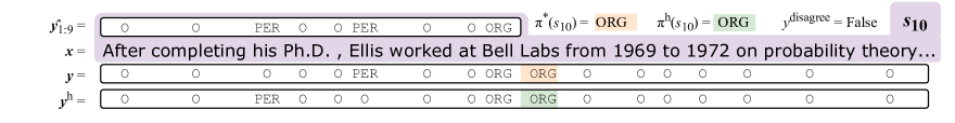
Figure 1: A named entity recognition example (from the Wikipedia page for Clarence Ellis). ${\boldsymbol{x}}$ is the input sentence and ${\boldsymbol{y}}$ is the (unobserved) ground truth. The predictor $\pi$ operates left-to-right and, in this example, is currently at state $s_{10}$ to tag the $10$th word; the state $s_{10}$ (highlighted in purple) combines ${\boldsymbol{x}}$ with $\hat{\boldsymbol{y}}_{1:9}$. The heuristic makes two errors at $t=4$ and $t=6$. The heuristic label at $t=10$ is $y^{h}_{10}=$ORG. Under Hamming loss, the cost at $t=10$ is minimized for $a=\texttt{ORG}$, which is therefore the expert action (if it were queried). The label that would be provided for $s_{10}$ to the difference classifier is $0$ because the two policies agree.

The challenge in learning the difference classifier is that it must learn based on one-sided feedback: if it predicts that the expert is likely to agree with the heuristic, the expert is not queried and the classifier cannot learn that it was wrong. We address this one-sided feedback problem using the Apple Tasting framework (Helmbold et al., 2000), in which errors (in predicting which apples are tasty) are only observed when a query is made (an apple is tasted). Learning in this way particularly important in the general case where the heuristic is likely not just to have high variance with respect to the expert, but is also statistically biased.

Experimentally (§ 4.5), we consider three structured prediction settings, each using a different type of heuristic feedback. We apply LeaQI to: English named entity recognition where the heuristic is a rule-based recognizer using gazetteers (Khashabi et al., 2018); English scientific keyphrase extraction, where the heuristic is an unsupervised method (Florescu and Caragea, 2017); and Greek part-of-speech tagging, where the heuristic is a small dictionary compiled from the training data (Zesch et al., 2008; Haghighi and Klein, 2006). In all three settings, the expert is a simulated human annotator. We train LeaQI on all three tasks using fixed BERT (Devlin et al., 2019) features, training only the final layer (because we are in the regime of small labeled data). The goal in all three settings is to minimize the number of words the expert annotator must label. In all settings, we’re able to establish the efficacy of LeaQI, showing that it can indeed provide significant label savings over using the expert alone and over several baselines and ablations that establish the importance of both the difference classifier and the Apple Tasting paradigm.

2 Background and Related Work

We review first the use of imitation learning for structured prediction, then online active learning, and finally applications of active learning to structured prediction and imitation learning problems.

2.1 Learning to Search

The learning to search approach to structured prediction casts the joint prediction problem of producing a complex output as a sequence of smaller classification problems (Ratnaparkhi, 1996; Collins and Roark, 2004; Daumé et al., 2009). For instance, in the named entity recognition example from Figure 1, an input sentence ${\boldsymbol{x}}$ is labeled one word at a time, left-to-right. At the depicted state ($s_{10}$), the model has labeled the first nine words and must next label the tenth word. Learning to search approaches assume access to an oracle policy $\pi^{\star}$, which provides the optimal label at every position.

In (interactive) imitation learning, we aim to imitate the behavior of the expert policy, $\pi^{\star}$, which provides the true labels. The learning to search view allows us to cast structured prediction as a (degenerate) imitation learning task, where states are (input, prefix) pairs, actions are operations on the output, and the horizon $T$ is the length of the sequence. States are denoted $s\in\mathcal{S}$, actions are denoted $a\in[K]$, where $[K]=\{1,\dots,K\}$, and the policy class is denoted $\Pi\subseteq[K]^{\mathcal{S}}$. The goal in learning is to find a policy $\pi\in\Pi$ with small loss on the distribution of states that it, itself, visits.

A popular imitation learning algorithm, DAgger (Ross et al., 2011), is summarized in Alg 1. In each iteration, DAgger executes a mixture policy and, at each visited state, queries the expert’s action. This produces a classification example, where the input is the state and the label is the expert’s action. At the end of each iteration, the learned policy is updated by training it on the accumulation of all generated data so far. DAgger is effective in practice and enjoys appealing theoretical properties; for instance, if the number of iterations $N$ is $\tilde{O}(T^{2}\log(1/\delta))$ then with probability at least $1-\delta$, the generalization error of the learned policy is $O(1/T)$ (Ross et al., 2011, Theorem 4.2).

Algorithm 1 $\text{DAgger}(\Pi,N,\langle\beta_{i}\rangle_{i=0}^{N},\pi^{\star})$

1:  initialize dataset $D=\{\}$

2:  initialize policy $\hat{\pi}_{1}$ to any policy in $\Pi$

3:  for $i=1\dots N$ do

4:     $\triangleright$ stochastic mixture policy

5:     Let $\pi_{i}=\beta_{i}\pi^{\star}+(1-\beta_{i})\hat{\pi}_{i}$

6:     Generate a $T$-step trajectory using $\pi_{i}$

7:     Accumulate data $D\leftarrow D\cup\{(s,\pi^{\star}(s))\}$ for all $s$ in those trajectories

8:     Train classifier $\hat{\pi}_{i+1}\in\Pi$ on $D$

9:  end for

10:  return  best (or random) $\hat{\pi}_{i}$

2.2 Active Learning

Active learning has been considered since at least the 1980s often under the name “selective sampling” (Rendell, 1986; Atlas et al., 1990). In agnostic online active learning for classification, a learner operates in rounds (e.g. Balcan et al., 2006; Beygelzimer et al., 2009, 2010). At each round, the learning algorithm is presented an example ${\boldsymbol{x}}$ and must predict a label; the learner must decide whether to query the true label. An effective margin-based approach for online active learning is provided by Cesa-Bianchi et al. (2006) for linear models. Their algorithm defines a sampling probability $\rho=b/(b+z)$, where $z$ is the margin on the current example, and $b>0$ is a hyperparameter that controls the aggressiveness of sampling. With probability $\rho$, the algorithm requests the label and performs a perceptron-style update.

Our approach is inspired by zhang2015active setting, where two labelers are available: a free weak labeler and an expensive strong labeler. Their algorithm minimizes queries to the strong labeler, by learning a difference classifier that predicts, for each example, whether the weak and strong labelers are likely to disagree. Their algorithm trains this difference classifier using an example-weighting strategy to ensure that its Type II error is kept small, establishing statistical consistency, and bounding its sample complexity.

This type of learning from one-sided feedback falls in the general framework of partial-monitoring games, a framework for sequential decision making with imperfect feedback. Apple Tasting is a type of partial-monitoring game (Littlestone and Warmuth, 1989), where, at each round, a learner is presented with an example ${\boldsymbol{x}}$ and must predict a label $\hat{y}\in\{-1,+1\}$. After this prediction, the true label is revealed only if the learner predicts $+1$. This framework has been applied in several settings, such as spam filtering and document classification with minority class distributions (Sculley, 2007). Sculley (2007) also conducts a through comparison of two methods that can be used to address the one-side feedback problem: label-efficient online learning (Cesa-Bianchi et al., 2006) and margin-based learning (Vapnik, 1982).

2.3 Active Imitation & Structured Prediction

In the context of structured prediction for natural language processing, active learning has been considered both for requesting full structured outputs (e.g. Thompson et al., 1999; Culotta and McCallum, 2005; Hachey et al., 2005) and for requesting only pieces of outputs (e.g. Ringger et al., 2007; Bloodgood and Callison-Burch, 2010). For sequence labeling tasks, Haertel et al. (2008) found that labeling effort depends both on the number of words labeled (which we model), plus a fixed cost for reading (which we do not).

In the context of imitation learning, active approaches have also been considered for at least three decades, often called “learning with an external critic” and “learning by watching” (Whitehead, 1991). More recently, Judah et al. (2012) describe RAIL, an active learning-for-imitation-learning algorithm akin to our ActiveDAgger baseline, but which in principle would operate with any underlying i.i.d. active learning algorithm (not just our specific choice of uncertainty sampling).

3 Our Approach: LeaQI

Our goal is to learn a structured prediction model with minimal human expert supervision, effectively by combining human annotation with a noisy heuristic. We present LeaQI to achieve this. As a concrete example, return to Figure 1: at $s_{10}$, $\pi$ must predict the label of the tenth word. If $\pi$ is confident in its own prediction, LeaQI can avoid any query, similar to traditional active learning. If $\pi$ is not confident, then LeaQI considers the label suggested by a noisy heuristic (here: ORG). LeaQI predicts whether the true expert label is likely to disagree with the noisy heuristic. Here, it predicts no disagreement and avoids querying the expert.

Algorithm 2 $\text{{LeaQI}}(\Pi,\mathcal{H},N,\pi^{\star},\pi^{\text{h}},b)$

1:  initialize dataset $D=\{\}$

2:  initialize policy $\pi_{1}$ to any policy in $\Pi$

3:  initialize difference dataset $S=\{\}$

4:  initialize difference classifier $h_{1}(s)=1~{}(\forall s)$

5:  for $i=1\dots N$ do

6:     Receive input sentence ${\boldsymbol{x}}$

7:     $\triangleright$ generate a $T$-step trajectory using $\pi_{i}$

8:     Generate output $\hat{\boldsymbol{y}}$ using $\pi_{i}$

9:     for each $s$ in $\hat{\boldsymbol{y}}$ do

10:        $\triangleright$ draw bernouilli random variable

11:        $Z_{i}\sim{\rm Bern}\left(\frac{b}{b+\textrm{certainty}(\pi_{i},s)}\right)$; see § 3.3

12:        if  $Z_{i}$ = 1 then

13:           $\triangleright$ set difference classifier prediction

14:           $\hat{d}_{i}=h_{i}(s)$

15:           if AppleTaste($s$, $\pi^{\text{h}}(s)$, $\hat{d}_{i}$) then

16:              $\triangleright$ predict agree query heuristic

17:              $D\leftarrow D\cup\left\{~{}\left(s,\pi^{\text{h}}(s)\right)~{}\right\}$

18:           else

19:              $\triangleright$ predict disagree query expert

20:              $D\leftarrow D\cup\left\{~{}\left(s,\pi^{\star}(s)\right)~{}\right\}$

21:              $d_{i}=\mathbbm{1}\big{[}\pi^{\star}(s)=\pi^{\text{h}}(s)\big{]}$

22:              $S\leftarrow S\cup\big{\{}~{}\big{(}s,\pi^{\text{h}}(s),\hat{d}_{i},d_{i}\big{)}~{}\big{\}}$

23:           end if

24:        end if

25:     end for

26:     Train policy $\pi_{i+1}\in\Pi$ on $D$

27:     Train difference classifier $h_{i+1}\in\mathcal{H}$ on $S$ to minimize Type II errors (see § 3.2)

28:  end for

29:  return  best (or random) $\pi_{i}$

3.1 Learning to Query for Imitation

Our algorithm, LeaQI, is specified in Alg 2. As input, LeaQI takes a policy class $\Pi$, a hypothesis class $\mathcal{H}$ for the difference classifier (assumed to be symmetric and to contain the “constant one” function), a number of episodes $N$, an expert policy $\pi^{\star}$, a heuristic policy $\pi^{\text{h}}$, and a confidence parameter $b>0$. The general structure of LeaQI follows that of DAgger, but with three key differences:

1. roll-in (7) is according to the learned policy (not mixed with the expert, as that would require additional expert queries),

2. actions are queried only if the current policy is uncertain at $s$ (12), and

3. the expert $\pi^{\star}$ is only queried if it is predicted to disagree with the heuristic $\pi^{\text{h}}$ at $s$ by the difference classifier, or if apple tasting method switches the difference classifier label (15; see § 3.2).

In particular, at each state visited by $\pi_{i}$, LeaQI estimates $z$, the certainty of $\pi_{i}$’s prediction at that state (see § 3.3). A sampling probability $\rho$ is set to $b/(b+z)$ where $z$ is the certainty, and so if the model is very uncertain then $\rho$ tends to zero, following (Cesa-Bianchi et al., 2006). With probability $\rho$, LeaQI will collect some label.

When a label is collected (12), the difference classifier $h_{i}$ is queried on state $s$ to predict if $\pi^{\star}$ and $\pi^{\text{h}}$ are likely to disagree on the correct action. (Recall that $h_{1}$ always predicts disagreement per 4.) The difference classifier’s prediction, $\hat{d}_{i}$, is passed to an apple tasting method in 15. Intuitively, most apple tasting procedures (including the one we use, STAP; see § 3.2) return $\hat{d}_{i}$, unless the difference classifier is making many Type II errors, in which case it may return $\lnot\hat{d}_{i}$.

Algorithm 3 $\text{AppleTaste\_STAP}(S,a^{\text{h}}_{i},\hat{d}_{i})$

1:  $\triangleright$ count examples that are action $a^{\text{h}}_{i}$

2:  let $t=\sum_{(\_,a,\_,\_)\in S}\mathbbm{1}[a^{\text{h}}_{i}=a]$

3:  $\triangleright$ count mistakes made on action $a^{\text{h}}_{i}$

4:  let $m=\sum_{(\_,a,\hat{d},d)\in S}\mathbbm{1}[\hat{d}\neq d\land a^{\text{h}}_{i}=a]$

5:  $w=$ $\frac{t}{|S|}$  $\triangleright$ percentage of time $a^{\text{h}}_{i}$ was seen

6:  if $w$ < 1 then

7:     $\triangleright$ skew distribution

8:     draw $r\sim\textit{Beta}(1-w,1)$

9:  else

10:     draw $r\sim\textit{Unifomm}(0,1)$

11:  end if

12:  return  $(d=1)\land(r\leq\sqrt{(m+1)/t})$

A target action is set to $\pi^{\text{h}}(s)$ if the apple tasting algorithm returns “agree” (17), and the expert $\pi^{\star}$ is only queried if disagreement is predicted (20). The state and target action (either heuristic or expert) are then added to the training data. Finally, if the expert was queried, then a new item is added to the difference dataset, consisting of the state, the heuristic action on that state, the difference classifier’s prediction, and the ground truth for the difference classifier whose input is $s$ and whose label is whether the expert and heuristic actually disagree. Finally, $\pi_{i+1}$ is trained on the accumulated action data, and $h_{i+1}$ is trained on the difference dataset (details in § 3.3).

There are several things to note about LeaQI:

1. If the current policy is already very certain, a expert annotator is never queried.

2. If a label is queried, the expert is queried only if the difference classifier predicts disagreement with the heuristic, or the apple tasting procedure flips the difference classifier prediction.

3. Due to apple tasting, most errors the difference classifier makes will cause it to query the expert unnecessarily; this is the “safe” type of error (increasing sample complexity but not harming accuracy), versus a Type II error (which leads to biased labels).

4. The difference classifier is only trained on states where the policy is uncertain, which is exactly the distribution on which it is run.

3.2 Apple Tasting for One-Sided Learning

The difference classifier $h\in\mathcal{H}$ must be trained (line 27) based on one-sided feedback (it only observes errors when it predicts “disagree“) to minimize Type II errors (it should only very rarely predict “agree” when the truth is “disagree”). This helps keep the labeled data for the learned policies unbiased. The main challenge here is that the feedback to the difference classifier is one-sided: that is, if it predicts “disagree” then it gets to see the truth, but if it predicts “agree” it never finds out if it was wrong. We use one of (Helmbold et al., 2000)’s algorithms, STAP (see Alg 3), which works by random sampling from apples that are predicted to not be tasted and tasting them anyway (line 12). Formally, STAP tastes apples that are predicted to be bad with probability $\sqrt{(m+1)/t}$, where $m$ is the number of mistakes, and $t$ is the number of apples tasted so far.

We adapt Apple Tasting algorithm STAP to our setting for controlling the number of Type II errors made by the difference classifier as follows. First, because some heuristic actions are much more common than others, we run a separate apple tasting scheme per heuristic action (in the sense that we count the number of error on this heuristic action rather than globally). Second, when there is significant action imbalance we find it necessary to skew the distribution from STAP more in favor of querying. We achieve this by sampling from a Beta distribution (generalizing the uniform), whose mean is shifted toward zero for more frequent heuristic actions. This increases the chance that Apple Tasting will have on finding bad apples error for each action (thereby keeping the false positive rate low for predicting disagreement).

3.3 Measuring Policy Certainty

In step 11, LeaQI must estimate the certainty of $\pi_{i}$ on $s$. Following Cesa-Bianchi et al. (2006), we implement this using a margin-based criteria. To achieve this, we consider $\pi$ as a function that maps actions to scores and then chooses the action with largest score. The certainty measure is then the difference in scores between the highest and second highest scoring actions:

$$\text{certainty}(\pi,s) =\max_{a}\pi(s,a)-\max_{a^{\prime}\neq a}\pi(s,a^{\prime})$$

3.4 Analysis

Theoretically, the main result for LeaQI is an interpretation of the main DAgger result(s). Formally, let $d_{\pi}$ denote the distribution of states visited by $\pi$, $C(s,a)\in[0,1]$ be the immediate cost of performing action $a$ in state $s$, $C_{\pi}(s)=\mathbb{E}_{a\sim\pi(s)}C(s,a)$, and the total expected cost of $\pi$ to be $J(\pi)=T\mathbb{E}_{s\sim d_{\pi}}C_{\pi}(s)$, where $T$ is the length of trajectories. $C$ is not available to a learner in an imitation setting; instead the algorithm observes an expert and minimizes a surrogate loss $\ell(s,\pi)$ (e.g., $\ell$ may be zero/one loss between $\pi$ and $\pi^{\star}$). We assume $\ell$ is strongly convex and bounded in $[0,1]$ over $\Pi$.

Given this setup assumptions, let $\epsilon_{\text{pol-approx}}=\min_{\pi\in\Pi}\frac{1}{N}\sum_{i=1}^{N}\mathbb{E}_{s\sim d_{\pi_{i}}}\ell(s,\pi)$ be the true loss of the best policy in hindsight, let $\epsilon_{\text{dc-approx}}=\min_{h\in\mathcal{H}}\frac{1}{N}\sum_{i=1}^{N}\mathbb{E}_{s\sim d_{\pi_{i}}}\textit{err}(s,h,\pi^{\star}(s)\neq\pi^{\text{h}}(s))$ be the true error of the best difference classifier in hindsight, and assuming that the regret of the policy learner is bounded by $\textit{reg}_{\text{pol}}(N)$ after $N$ steps, Ross et al. (2011) shows the following:

Theorem 1 (Thm 4.3 of Ross et al. (2011)).

After $N$ episodes each of length $T$, under the assumptions above, with probability at least $1-\delta$ there exists a policy $\pi\in\pi_{1:N}$ such that:

$$\mathbb{E}_{s\sim d_{\pi}}\ell(s,\pi)\leq$$

$$\quad\epsilon_{\text{pol-approx}}+\textit{reg}_{\text{pol}}(N)+\sqrt{(2/N)\log(1/\delta)}$$

Task	Named Entity Recognition	Keyphrase Extraction	Part of Speech Tagging
Language	English (en)	English (en)	Modern Greek (el)
Dataset	CoNLL’03 (Tjong Kim Sang and De Meulder, 2003)	SemEval 2017 Task 10 (Augenstein et al., 2017)	Universal Dependencies Nivre (2018)
# Ex	$14,987$	$2,809$	$1,662$
Avg. Len	$14.5$	$26.3$	$25.5$
# Actions	$5$	$2$	$17$
Metric	Entity F-score	Keyphrase F-score	Per-tag accuracy
Features	English BERT (Devlin et al., 2019)	SciBERT (Beltagy et al., 2019)	M-BERT (Devlin et al., 2019)
Heuristic	String matching against an offline gazeteer of entities from Khashabi et al. (2018)	Output from an unsupervised keyphrase extraction model Florescu and Caragea (2017)	Dictionary from Wiktionary, similar to Zesch et al. (2008) and Haghighi and Klein (2006)
Heur Quality	P $88\%$, R $27\%$, F $41\%$	P $20\%$, R $44\%$, F $27\%$	$10\%$ coverage, $67\%$ acc

Table 1: An overview of the three tasks considered in experiments.

This holds regardless of how $\pi_{1:N}$ are trained (26). The question of how well LeaQI performs becomes a question of how well the combination of uncertainty-based sampling and the difference classifier learn. So long as those do a good job on their individual classification tasks, DAgger guarantees that the policy will do a good job. This is formalized below, where $Q^{\star}(s,a)$ is the best possible cumulative cost (measured by $C$) starting in state $s$ and taking action $a$:

Theorem 2 (Theorem 2.2 of Ross et al. (2011)).

Let $u$ be such that $Q^{\star}(s,a)-Q^{\star}(s,\pi^{\star}(s))\leq u$ for all $a$ and all $s$ with $d_{\pi}(s)>0$; then for some $\pi\in\pi_{1:N}$, as $N\rightarrow\infty$:

$$J(\pi) \leq J(\pi^{\star})+uT\epsilon_{\text{pol-approx}}$$

Here, $u$ captures the most long-term impact a single decision can have; for example, for average Hamming loss, it is straightforward to see that $u=\frac{1}{T}$ because any single mistake can increase the number of mistakes by at most $1$. For precision, recall and F-score, $u$ can be as large as one in the (rare) case that a single decision switches from one true positive to no true positives.

4 Experiments

The primary research questions we aim to answer experimentally are:

1. Does uncertainty-based active learning achieve lower query complexity than passive learning in the learning to search settings?

2. Does learning a difference classifier improve query efficiency over active learning alone?

3. Does Apple Tasting successfully handle the problem of learning from one-sided feedback?

4. Is the approach robust to cases where the noisy heuristic is uncorrelated with the expert?

5. Is casting the heuristic as a policy more effective than using its output as features?

To answer these questions, we conduct experiments on three tasks (see Table 1): English named entity recognition, English scientific keyphrase extraction, and low-resource part of speech tagging on Modern Greek (el), selected as a low-resource setting.

4.1 Algorithms and Baselines

In order to address the research questions above, we compare LeaQI to several baselines. The baselines below compare our approach to previous methods:

DAgger.

Passive DAgger (Alg 1)

ActiveDAgger.

An active variant of DAgger that asks for labels only when uncertain. (This is equivalent to LeaQI, but with neither the difference classifier nor apple tasting.)

DAgger+Feat.

DAgger with the heuristic policy’s output appended as an input feature.

ActiveDAgger+Feat.

ActiveDAgger with the heuristic policy as a feature.

The next set of comparisons are explicit ablations:

LeaQI+NoAT

LeaQI with no apple tasting.

LeaQI+NoisyHeur.

LeaQI, but where the heuristic returns a label uniformly at random.

The baselines and LeaQI share a linear relationship. DAgger is the baseline algorithm used by all algorithms described above but it is very query inefficient with respect to an expert annotator. ActiveDAgger introduces active learning to make DAgger more query efficient; the delta to the previous addresses Q1. LeaQI+NoAT introduces the difference classifier; the delta addresses Q2. LeaQI adds apple tasting to deal with one-sided learning; the delta addresses Q3. Finally, LeaQI+NoisyHeur. (vs LeaQI) addresses Q4 and the +Feat variants address Q5.

4.2 Data and Representation

For named entity recognition, we use training, validation, and test data from CoNLL’03 (Tjong Kim Sang and De Meulder, 2003), consisting of IO tags instead of BIO tags (the “B” tag is almost never used in this dataset, so we never attempt to predict it) over four entity types: Person, Organization, Location, and Miscellaneous. For part of speech tagging, we use training and test data from modern Greek portion of the Universal Dependencies (UD) treebanks (Nivre, 2018), consisting of 17 universal tags. For keyphrase extraction, we use training, validation, and test data from SemEval 2017 Task 10 (Augenstein et al., 2017), consisting of IO tags (we use one “I” tag for all three keyphrase types).

In all tasks, we implement both the policy and difference classifier by fine-tuning the last layer of a BERT embedding representation (Devlin et al., 2019). More specifically, for a sentence of length $T$, $w_{1},\dots,w_{T}$, we first compute BERT embeddings for each word, ${\boldsymbol{x}}_{1},\dots,{\boldsymbol{x}}_{T}$ using the appropriate BERT model: English BERT and M-BERT for named entity and part-of-speech, respectively, and SciBERT (Beltagy et al., 2019) for keyphrase extraction. We then represent the state at position $t$ by concatenating the word embedding at that position with a one-hot representation of the previous action: $s_{t}=[{\boldsymbol{w}}_{t};\text{onehot}(a_{t-1})]$. This feature representation is used both for learning the labeling policy and also learning the difference classifier.

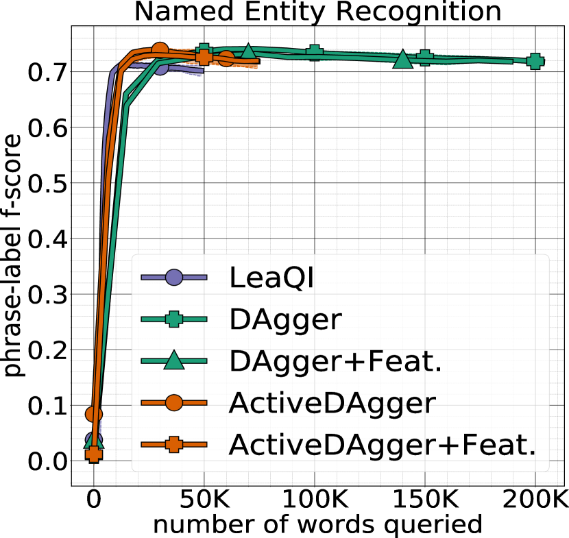
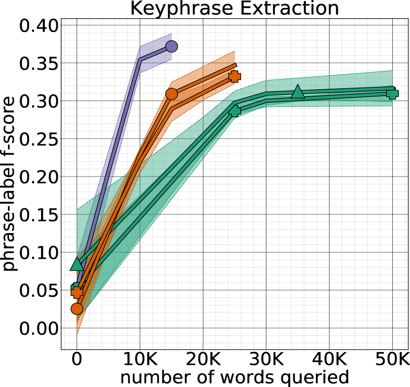
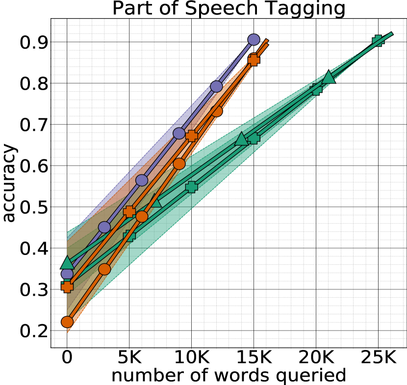
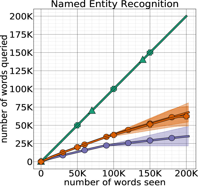
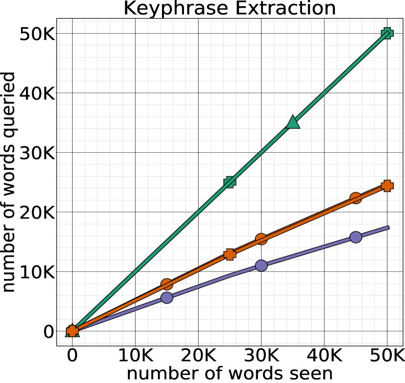
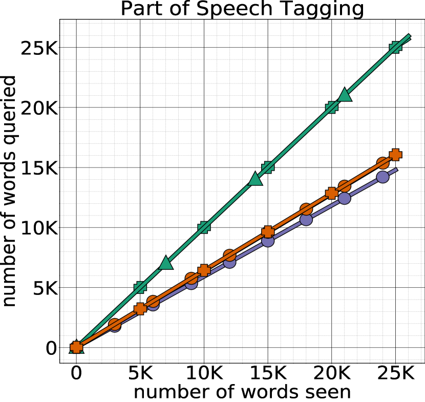
Figure 2: Empirical evaluation on three tasks: (left) named entity recognition, (middle) keyphrase extraction and (right) part of speech tagging. The top rows shows performance (f-score or accuracy) with respect to the number of queries to the expert. The bottom row shows the number of queries as a function of the number of words seen.

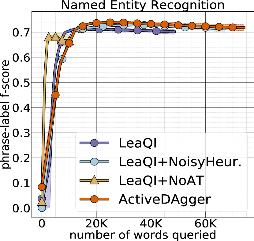
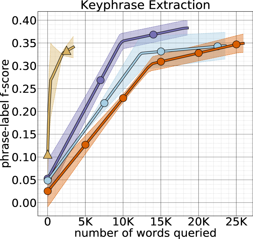
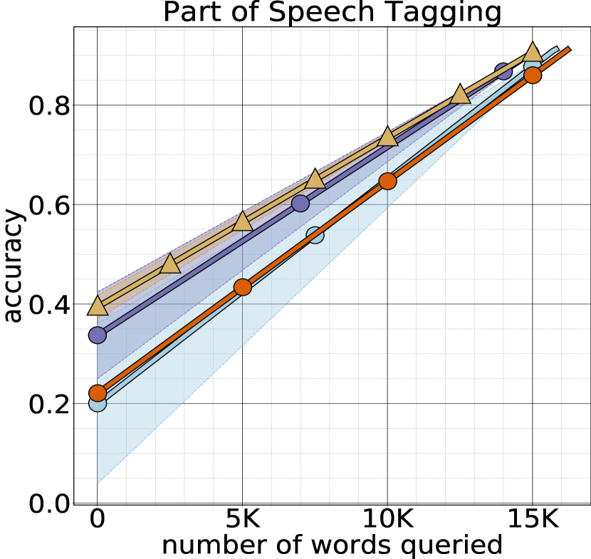
Figure 3: Ablation results on (left) named entity recognition, (middle) keyphrase extraction and (right) part of speech tagging. In addition to LeaQI and DAgger (copied from Figure 2), these graphs also show LeaQI+NoAT (apple tasting disabled), and LeaQI+NoisyHeur. (a heuristic that produces labels uniformly at random).

4.3 Expert Policy and Heuristics

In all experiments, the expert $\pi^{\star}$ is a simulated human annotator who annotates one word at a time. The expert returns the optimal action for the relevant evaluation metric (F-score for named entity recognition and keyphrase extraction, and accuracy for part-of-speech tagging). We take the annotation cost to be the total number of words labeled.

The heuristic we implement for named entity recognition is a high-precision gazeteer-based string matching approach. We construct this by taking a gazeteer from Wikipedia using the CogComp framework (Khashabi et al., 2018), and use FlashText (Singh, 2017) to label the dataset. This heuristic achieves a precision of $0.88$, recall of $0.27$ and F-score of $0.41$ on the training data.

The keyphrase extraction heuristic is the output of an “unsupervised keyphrase extraction” approach (Florescu and Caragea, 2017). This system is a graph-based approach that constructs word-level graphs incorporating positions of all word occurrences information; then using PageRank to score the words and phrases. This heuristic achieves a precision of $0.20$, recall of $0.44$ and F-score of $0.27$ on the training data.

The part of speech tagging heuristic is based on a small dictionary compiled from Wiktionary. Following Haghighi and Klein (2006) and Zesch et al. (2008), we extract this dictionary using Wiktionary as follows: for word $w$ in our training data, we find the part-of-speech $y$ by querying Wiktionary. If $w$ is in Wikitionary, we convert the Wikitionary part of speech tag to a Universal Dependencies tag (see § A.1), and if word $w$ is not in Wiktionary, we use a default label of “X”. Furthermore, if word $w$ has multiple parts of speech, we select the first part of speech tag in the list. The label “X” is chosen $90\%$ of the time. For the remaining $10\%$, the heuristic achieves an accuracy of $0.67$ on the training data.

4.4 Experimental Setup

Our experimental setup is online active learning. We make a single pass over a dataset, and the goal is to achieve an accurate system as quickly as possible. We measure performance (accuracy or F-score) after every $1000$ words ($\approx 50$ sentences) on heldout test data, and produce error bars by averaging across three runs and reporting standard deviations.

Hyperparameters for DAgger are optimized using grid-search on the named entity recognition training data and evaluated on development data. We then fix DAgger hyperparameters for all other experiments and models. The difference classifier hyperparameters are subsequently optimized in the same manner. We fix the difference classifier hyperparameters for all other experiments.

4.5 Experimental Results

The main results are shown in the top two rows of Figure 2; ablations of LeaQI are shown in Figure 3. In Figure 2, the top row shows traditional learning curves (performance vs number of queries), and the bottom row shows the number of queries made to the expert as a function of the total number of words seen.

Active vs Passive (Q1).

In all cases, we see that the active strategies improve on the passive strategies; this difference is largest in keyphrase extraction, middling for part of speech tagging, and small for NER. While not surprising given previous successes of active learning, this confirms that it is also a useful approach in our setting. As expected, the active algorithms query far less than the passive approaches, and LeaQI queries the least.

Heuristic as Features vs Policy (Q5).

We see that while adding the heuristic’s output as a feature can be modestly useful, it is not uniformly useful and, at least for keyphrase extraction and part of speech tagging, it is not as effective as LeaQI. For named entity recognition, it is not effective at all, but this is also a case where all algorithms perform essentially the same. Indeed, here, LeaQI learns quickly with few queries, but never quite reaches the performance of ActiveDAgger. This is likely due to the difference classifier becoming overly confident too quickly, especially on the “O” label, given the (relatively well known) oddness in mismatch between development data and test data on this dataset.

Difference Classifier Efficacy (Q2).

Turning to the ablations (Figure 3), we can address Q2 by comparing the ActiveDAgger curve to the LeaQI+NoAT curve. Here, we see that on NER and keyphrase extraction, adding the difference classifier without adding apple tasting results in a far worse model: it learns very quickly but plateaus much lower than the best results. The exception is part of speech tagging, where apple tasting does not seem necessary (but also does not hurt). Overall, this essentially shows that without controlling Type II errors, the difference classifier on it’s own does not fulfill its goals.

Apple Tasting Efficacy (Q3).

Also considering the ablation study, we can compare LeaQI+NoAT with LeaQI. In the case of part of speech tagging, there is little difference: using apple tasting to combat issues of learning from one sided feedback neither helps nor hurts performance. However, for both named entity recognition and keyphrase extraction, removing apple tasting leads to faster learning, but substantially lower final performance (accuracy or f-score). This is somewhat expected: without apple tasting, the training data that the policy sees is likely to be highly biased, and so it gets stuck in a low accuracy regime.

Robustness to Poor Heuristic (Q4).

We compare LeaQI+NoisyHeur to ActiveDAgger. Because the heuristic here is useless, the main hope is that it does not degrade performance below ActiveDAgger. Indeed, that is what we see in all three cases: the difference classifier is able to learn quite quickly to essentially ignore the heuristic and only rely on the expert.

5 Discussion and Limitations

In this paper, we considered the problem of reducing the number of queries to an expert labeler for structured prediction problems. We took an imitation learning approach and developed an algorithm, LeaQI, which leverages a source that has low-quality labels: a heuristic policy that is suboptimal but free. To use this heuristic as a policy, we learn a difference classifier that effectively tells LeaQI when it is safe to treat the heuristic’s action as if it were optimal. We showed empirically—across Named Entity Recognition, Keyphrase Extraction and Part of Speech Tagging tasks—that the active learning approach improves significantly on passive learning, and that leveraging a difference classifier improves on that.

1. In some settings, learning a difference classifier may be as hard or harder than learning the structured predictor; for instance if the task is binary sequence labeling (e.g., word segmentation), minimizing its usefulness.

2. The true labeling cost is likely more complicated than simply the number of individual actions queried to the expert.

Despite these limitations, we hope that LeaQI provides a useful (and relatively simple) bridge that can enable using rule-based systems, heuristics, and unsupervised models as building blocks for more complex supervised learning systems. This is particularly attractive in settings where we have very strong rule-based systems, ones which often outperform the best statistical systems, like coreference resolution (Lee et al., 2011), information extraction (Riloff and Wiebe, 2003), and morphological segmentation and analysis (Smit et al., 2014).

Supplementary Material For:
Active Imitation Learing with Noisy Guidance

Appendix A Experimental Details:

A.1 Wiktionary to Universal Dependencies

POS Tag Source	Greek, Modern (el) Wiktionary	Universal Dependencies
	adjective	ADJ
	adposition	ADP
	preposition	ADP
	adverb	ADV
	auxiliary	AU
	coordinating conjunction	CCONJ
	determiner	DET
	interjection	INTJ
	noun	NOUN
	numeral	NUM
	particle	PART
	pronoun	PRON
	proper noun	pROPN
	punctuation	PUNCT
	subordinating conjunction	SCONJ
	symbol	SYM
	verb	VERB
	other	X
	article	DET
	conjunction	PART

Table 2: Conversion between Greek, Modern (el) Wiktionary POS tags and Universal Dependencies POS tags.

A.2 Hyperparameters

Here we provide a table of all of hyperparameters we considered for LeaQI and baselines models. (see section 4.4)

Table 3: Hyperparameters

Hyperparameter	Values Considered	Final Value
Policy Learning rate	$10^{-3},10^{-4},10^{-5},10^{-6},5.5\cdot 10^{-6},10^{-6}$	$10^{-6}$
Difference Classifier Learning rate $h$	$10^{-1},10^{-2},10^{-3},10^{-4}$	$10^{-2}$
Confidence parameter (b)	$5.0\cdot 10^{-1},10\cdot 10^{-1},15\cdot 10^{-1}$	$5.0\cdot 10^{-1}$

A.3 Ablation Study Difference Classifier Learning Rate

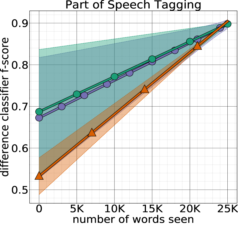
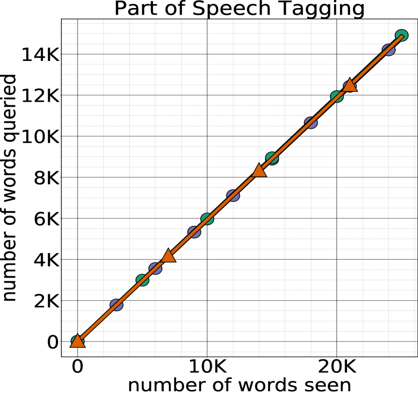
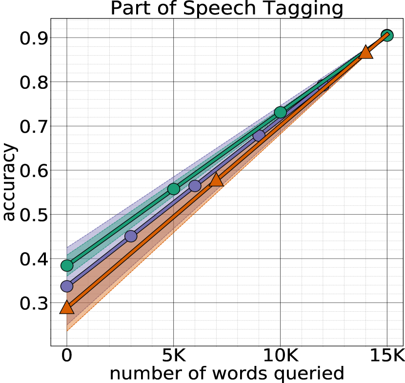
Figure 4: (top-row) English keyphrase extraction and (bottom-row) low-resource language part of speech tagging on Greek, Modern (el). We show the performance of using different learning for the difference classifier $h$. These plots indicate that their is small difference in performance depending on the difference classifier learning rate.

A.4 Ablation Study Confidence Parameter: $b$

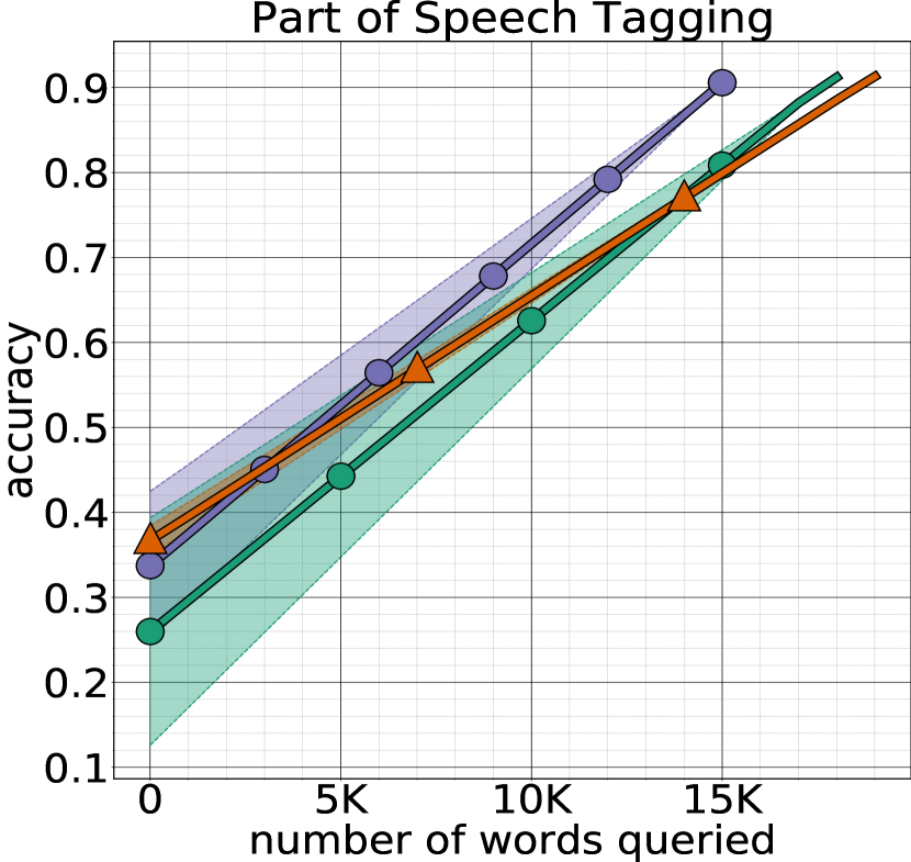
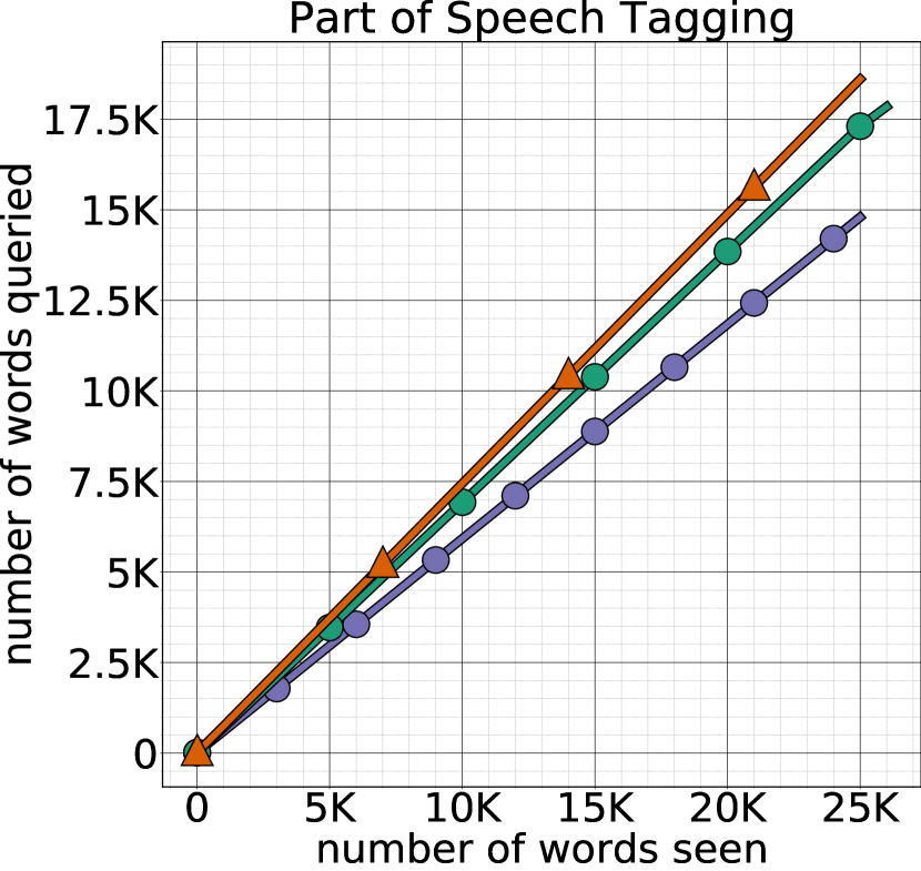
Figure 5: (top-row) English keyphrase extraction and (bottom-row) low-resource language part of speech tagging on Greek, Modern (el). We show the performance of using difference confidence parameters $b$. These plots indicate that our model is robust to difference confidence parameters.

References

- Atlas et al. (1990) Les E Atlas, David A Cohn, and Richard E Ladner. 1990. Training connectionist networks with queries and selective sampling. In NeurIPS.
- Augenstein et al. (2017) Isabelle Augenstein, Mrinal Das, Sebastian Riedel, Lakshmi Vikraman, and Andrew McCallum. 2017. Semeval 2017 task 10: Scienceie - extracting keyphrases and relations from scientific publications. In Proceedings of the 11th International Workshop on Semantic Evaluation (SemEval-2017).
- Balcan et al. (2006) Nina Balcan, Alina Beygelzimer, and John Langford. 2006. Agnostic active learning. In ICML.
- Beltagy et al. (2019) Iz Beltagy, Kyle Lo, and Arman Cohan. 2019. Scibert: Pretrained language model for scientific text. In EMNLP.
- Bengio et al. (2015) Samy Bengio, Oriol Vinyals, Navdeep Jaitly, and Noam Shazeer. 2015. Scheduled sampling for sequence prediction with recurrent neural networks. In NeurIPS.
- Beygelzimer et al. (2009) Alina Beygelzimer, Sanjoy Dasgupta, , and John Langford. 2009. Importance weighted active learning. In ICML.
- Beygelzimer et al. (2010) Alina Beygelzimer, Daniel Hsu, John Langford, and Tong Zhang. 2010. Agnostic active learning without constraints. In NeurIPS.
- Bloodgood and Callison-Burch (2010) Michael Bloodgood and Chris Callison-Burch. 2010. Bucking the trend: Large-scale cost-focused active learning for statistical machine translation. In ACL.
- Cesa-Bianchi et al. (2006) Nicolò Cesa-Bianchi, Claudio Gentile, and Luca Zaniboni. 2006. Worst-case analysis ofselective sampling for linear classification. JMLR.
- Collins and Roark (2004) Michael Collins and Brian Roark. 2004. Incremental parsing with the perceptron algorithm. In ACL.
- Culotta and McCallum (2005) Aron Culotta and Andrew McCallum. 2005. Reducing labeling effort for structured prediction tasks. In AAAI.
- Daumé et al. (2009) Hal Daumé, III, John Langford, and Daniel Marcu. 2009. Search-based structured prediction. Machine Learning Journal.
- Devlin et al. (2019) Jacob Devlin, Ming-Wei Chang, Kenton Lee, and Kristina Toutanova. 2019. BERT: Pre-training of deep bidirectional transformers for language understanding. In NAACL.
- Florescu and Caragea (2017) Corina Florescu and Cornelia Caragea. 2017. PositionRank: An unsupervised approach to keyphrase extraction from scholarly documents. In ACL.
- Hachey et al. (2005) Ben Hachey, Beatrice Alex, and Markus Becker. 2005. Investigating the effects of selective sampling on the annotation task. In CoNLL.
- Haertel et al. (2008) Robbie Haertel, Eric K. Ringger, Kevin D. Seppi, James L. Carroll, and Peter McClanahan. 2008. Assessing the costs of sampling methods in active learning for annotation. In ACL.
- Haghighi and Klein (2006) Aria Haghighi and Dan Klein. 2006. Prototype-driven learning for sequence models.
- Helmbold et al. (2000) David P. Helmbold, Nicholas Littlestone, and Philip M. Long. 2000. Apple tasting. Information and Computation.
- Judah et al. (2012) Kshitij Judah, Alan Paul Fern, and Thomas Glenn Dietterich. 2012. Active imitation learning via reduction to iid active learning. In AAAI.
- Khashabi et al. (2018) Daniel Khashabi, Mark Sammons, Ben Zhou, Tom Redman, Christos Christodoulopoulos, Vivek Srikumar, Nicholas Rizzolo, Lev Ratinov, Guanheng Luo, Quang Do, Chen-Tse Tsai, Subhro Roy, Stephen Mayhew, Zhili Feng, John Wieting, Xiaodong Yu, Yangqiu Song, Shashank Gupta, Shyam Upadhyay, Naveen Arivazhagan, Qiang Ning, Shaoshi Ling, and Dan Roth. 2018. CogCompNLP: Your swiss army knife for NLP. In LREC.
- Leblond et al. (2018) Rémi Leblond, Jean-Baptiste Alayrac, Anton Osokin, and Simon Lacoste-Julien. 2018. SEARNN: Training RNNs with global-local losses. In ICLR.
- Lee et al. (2011) Heeyoung Lee, Yves Peirsman, Angel Chang, Nathanael Chambers, Mihai Surdeanu, and Dan Jurafsky. 2011. Stanford’s multi-pass sieve coreference resolution system at the conll-2011 shared task. In Proceedings of the Fifteenth Conference on Computational Natural Language Learning: Shared Task.
- Littlestone and Warmuth (1989) N. Littlestone and M. K. Warmuth. 1989. The weighted majority algorithm. In Proceedings of the 30th Annual Symposium on Foundations of Computer Science.
- Nivre (2018) Joakim et. al Nivre. 2018. Universal dependencies v2.5. LINDAT/CLARIN digital library at the Institute of Formal and Applied Linguistics, Charles University.
- Ratnaparkhi (1996) Adwait Ratnaparkhi. 1996. A maximum entropy model for part-of-speech tagging. In EMNLP.
- Rendell (1986) Larry Rendell. 1986. A general framework for induction and a study of selective induction. Machine Learning Journal.
- Riloff and Wiebe (2003) Ellen Riloff and Janyce Wiebe. 2003. Learning extraction patterns for subjective expressions. In EMNLP.
- Ringger et al. (2007) Eric Ringger, Peter McClanahan, Robbie Haertel, George Busby, Marc Carmen, James Carroll, Kevin Seppi, and Deryle Lonsdale. 2007. Active learning for part-of-speech tagging: Accelerating corpus annotation. In Proceedings of the Linguistic Annotation Workshop.
- Ross et al. (2011) Stéphane Ross, Geoff J. Gordon, and J. Andrew Bagnell. 2011. A reduction of imitation learning and structured prediction to no-regret online learning. In AI-Stats.
- Sculley (2007) David Sculley. 2007. Practical learning from one-sided feedback. In KDD.
- Singh (2017) Vikash Singh. 2017. Replace or retrieve keywords in documents at scale. CoRR, abs/1711.00046.
- Smit et al. (2014) Peter Smit, Sami Virpioja, Stig-Arne Grönroos, and Mikko Kurimo. 2014. Morfessor 2.0: Toolkit for statistical morphological segmentation. In EACL.
- Thompson et al. (1999) Cynthia A. Thompson, Mary Elaine Califf, and Raymond J. Mooney. 1999. Active learning for natural language parsing and information extraction. In ICML.
- Tjong Kim Sang and De Meulder (2003) Erik F. Tjong Kim Sang and Fien De Meulder. 2003. Introduction to the CoNLL-2003 shared task: Language-independent named entity recognition. In NAACL/HLT.
- Vapnik (1982) Vladimir Vapnik. 1982. Estimation of Dependences Based on Empirical Data: Springer Series in Statistics (Springer Series in Statistics). Springer-Verlag, Berlin, Heidelberg.
- Whitehead (1991) Steven Whitehead. 1991. A study of cooperative mechanisms for faster reinforcement learning. Technical report, University of Rochester.
- Zesch et al. (2008) Torsten Zesch, Christof Müller, and Iryna Gurevych. 2008. Extracting lexical semantic knowledge from Wikipedia and Wiktionary. In LREC.
- Zhang and Chaudhuri (2015) Chicheng Zhang and Kamalika Chaudhuri. 2015. Active learning from weak and strong labelers. In NeurIPS.