Relaxation of the collective magnetization of a dense 3D array of interacting dipolar S=3 atoms

Abstract

We report on measurements of the dynamics of the collective spin length (total magnetization) and spin populations in an almost unit filled lattice system comprising about $10^{4}$ spin $S=3$ chromium atoms, under the effect of dipolar interactions. The observed spin population dynamics is unaffected by the use of a spin echo, and fully consistent with numerical simulations of the $S=3$ XXZ spin model. On the contrary, the observed spin length decays slower than in simulations, and surprisingly reaches a small but nonzero asymptotic value within the longest timescale. Our findings show that spin coherences are sensitive probes to systematic effects affecting quantum many-body behavior that cannot be diagnosed by merely measuring spin populations.

Synthetic atom-based materials are emerging as unique quantum laboratories for the exploration of collective behaviors in interacting many-body systemsGross and Bloch (2017). In particular both electric and magnetic dipolar gases featuring long range spin-spin interactions are opening great opportunities for the exploration of quantum magnetism in regimes inaccessible to gases interacting via purely contact interactions Bohn et al. (2017).

While electric dipolar interactions are fundamentally stronger and have led to important breakthroughs as demonstrated by recent experiments using KRb molecules in 3D lattices Yan et al. (2013) and Rydberg atoms in bulk gases Signoles et al. (2019) as well as in optical tweezers arrays Bernien et al. (2017); Browaeys and Lahaye (2020); de Léséleuc et al. (2019); Schauß et al. (2015, 2012); Keesling et al. (2019), magnetic quantum dipoles offer complementary unique opportunities for quantum simulations. For example, they provide the possibility to trap low entropy and dense macroscopic arrays of $S>1/2$ atoms in close to unit filled 3D optical lattice potentials where truly collective many-body behavior manifests itself. Under these conditions it is possible to study spin models with large spins Lahaye et al. (2009); de Paz et al. (2013, 2016) which cost exponentially more resources to classically simulate Hallgren et al. (2013) than conventional $S=1/2$ models of magnetism. These capabilities have started to be explored in experiments working both with bosonic chromium and fermionic erbium atoms in 3D lattices de Paz et al. (2013, 2016); Lepoutre et al. (2019); Fersterer et al. (2019); Patscheider et al. (2020), which have observed already signatures of rich many-body dynamics including quantum thermalization and the buildup of many-body correlations. However, so far all the information has only been extracted from measurements of spin populations without direct access to quantum coherences, which contain key signatures of the underlying quantum dynamics Yan et al. (2013); Signoles et al. (2019).

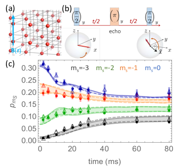
Figure 1: (a) The experimental system consists of a 3D array of dipolar Cr atoms, with a spatially varying magnetic field $B({\bf r})$. (b) Experimental RF sequence: Cr atoms are initialized in the $m_{s}=-3$ spin state and rotated by the first $\pi/2$ pulse to align with the $x$ direction; the 2nd $\pi/2$ pulse is used to measure the spin length. Due to magnetic noise the collective spin length makes an angle $\phi$ with respect to Ox when this second pulse is imparted. We impart or not an echo pulse using an additional $\pi$ pulse at half the evolution time $t/2$. (c) Time-evolution of the fractional populations $p_{m_{s}}$ of 4 $m_{s}$ spin components, with and without spin echo (full circles and empty triangles respectively). Each data point corresponds to the average of 10 realizations. Error bars correspond to statistical uncertainties. The solid (dashed) lines show the numerical results obtained with GDTWA for spin dynamics with (without) spin echo, for a lattice with unit filling and $B_{Q}/h=-4$ Hz. From bottom to top: $m_{s}=-3$ (black),$m_{s}=-2$ (green), $m_{s}=-1$ (orange), $m_{s}=0$ (blue). The colored bands in the GDTWA calculations account for a $5\%$ experimental error in the first pulse area.

Here we make a step forward and report time-resolved measurements of the spin coherence and also populations of a many-body strongly interacting spin $S=3$ dipolar gas of ⁵²Cr atoms in a deep 3D lattice. The spin coherence is extracted by measurements of the collective transverse magnetization of the gas, ${J_{\bot}}$, via Ramsey spectroscopy. Since the longitudinal magnetization remains zero at all times, the measurement of the transverse magnetization can also be seen as a measurement of the total magnetization (or the collective spin length) of the ensemble. The system is initially prepared in a far-from-equilibrium spin coherent state with maximal transverse magnetization ${J_{\bot}}=SN$, which is let to evolve due to magnetic dipolar couplings. Our experimental protocol includes a spin-echo pulse at the middle of the dynamics to reduce the effect of magnetic field inhomogeneities on the transverse magnetization dynamics.

In agreement with previous results Lepoutre et al. (2019); Fersterer et al. (2019); Patscheider et al. (2020), we find that the spin population dynamics is well captured by a semiclassical method, referred to as the generalized discrete truncated Wigner approximation (GDTWA), based on a discrete Monte Carlo sampling in phase space Zhu et al. (2019); Schachenmayer et al. (2015). In addition, we find that spin dynamics is barely affected by the spin echo. However, we observe that the observed transverse magnetization not only decays at a slower rate than the one expected from a pure spin XXZ model but also saturates at a non-zero value, behavior that is inconsistent with numerical expectations. We attribute the difference to effects not included in the pure spin model such as tunneling induced by lattice heating. We provide toy model simulations that support this claim. Our observations highlight the relevance of quantum coherence to characterize many-body phenomena.

Our experimental platform differs from previous studies on the transverse magnetization of ensembles of dipolar particles Yan et al. (2013); Signoles et al. (2019) in that it consists of a high density ordered array of S=3 spin particles. It is obtained by loading a ⁵²Cr BEC in a 3D optical lattice deep into the Mott regime. We obtain typically $N_{S}=10^{4}$ atoms close to unit filling (see Lepoutre et al. (2019) for details). Initially the sample is prepared in a spin coherent state, with all spins in the maximally stretched state $m_{S}=-3$ and aligned with the external magnetic field B. Spin dynamics is triggered by aligning all spins at $t=0$ along a direction orthogonal to B, by the use of a resonant RF pulse (See Fig. 1). We measure the dynamical evolution of the seven spin populations $N_{m_{S}}$ in the basis set by the external magnetic field through Stern-Gerlach separation. We also probe the collective spin length (total magnetization) $\mathbf{J}=\sum_{i=1}^{N_{S}}\mathbf{S}_{i}$ which has a norm $\left|\left|\mathbf{J}\right|\right|=\sqrt{\left<J_{x}\right>^{2}+\left<J_{y}\right>^{2}+\left<J_{z}\right>^{2}}$ ranging from $0$ to $3N_{S}$. The maximal value is reached for the maximally polarized state, e.g. the initial spin state. In the following we will use normalized quantities: $\mathbf{j}=\mathbf{J}/N_{S}$ and $\ell=\left|\left|\mathbf{j}\right|\right|$.

To measure $\ell$ we use a Ramsey protocol, in which a second $\pi/2$ rotation is imparted just before population measurements (See Fig. 1). In the rotating frame (turning around $z$ at the RF frequency), RF pulses ensure rotation of the spins around an axis called $y$. After the first $\pi/2$ pulse, $\mathbf{j}_{t=0}\propto\hat{x}$. During the spin dynamics, fluctuations of the external magnetic field make $\mathbf{j}$ rotate in the $xy$ plane. We denote $\phi(t)$ the angle between $\mathbf{j}$ and $\hat{x}$ and use it to define a new basis $XYz$ where $\mathbf{j}\parallel\hat{X}$ i.e. $\ell=<\hat{j}_{X}>$. Since the second $\pi/2$ pulse again rotates spins around $y$, the normalized magnetization measured by the Stern and Gerlach protocol, denoted as $M_{z}$, corresponds to a measurement of $\hat{j}_{x}=\cos\left(\phi\right)\hat{j}_{X}-\sin\left(\phi\right)\hat{j}_{Y}$ after a Ramsey sequence. Since $\phi(t)$ is different trial to trial, this random phase generates a net dephasing which is useful to extract the net spin length.

If one can neglect tunneling, the prepared ensemble of $N_{S}$ coupled spins, which are pinned at the individual sites of a 3D lattice, evolve under a pure spin model. In the presence of an external magnetic $B$ field strong enough to generate Zeeman splittings larger than nearest-neighbor dipolar interactions, the dynamics is described by the following XXZ spin model de Paz et al. (2013):

$$\hat{H}_{\rm dd}=\sum_{i>j}^{N_{S}}V_{ij}\left[\hat{S}_{i}^{z}\hat{S}_{j}^{z}-\frac{1}{2}\left(\hat{S}_{i}^{x}\hat{S}_{j}^{x}+\hat{S}_{i}^{y}\hat{S}_{j}^{y}\right)\right]$$ (1)

$V_{i,j}=\frac{\mu_{0}(g\mu_{B})^{2}}{4\pi}\left(\frac{1-3\cos^{2}\theta_{i,j}}{r_{i,j}^{3}}\right)$, with $\mu_{0}$ the magnetic permeability of vacuum, $g\simeq 2$ the Landé factor, and $\mu_{B}$ the Bohr magneton. The sum runs over all pairs of particles ($i$,$j$). $r_{i,j}$ is the distance between atoms, $\theta_{i,j}$ the angle between their inter-atomic axis and the external magnetic field assumed to be along the $z$ axis, and ${\bf{\hat{S}}}_{i}=\{\hat{S}_{i}^{x},\hat{S}_{i}^{y},\hat{S}_{i}^{z}\}$ are spin-3 angular momentum operators, associated with atom $i$ som . For an ensemble of dipolar spins, the normalized spin length $\ell$ decreases as a result of interactions, which at short time follows the form:

$$\ell(t)=3-\frac{81t^{2}V_{\rm{eff}}^{2}}{16\hbar^{2}},$$ (2)

where $V_{\rm{eff}}/h=\sqrt{1/N_{S}\times\sum_{i\neq j}^{N_{S}}V_{ij}^{2}}/h\simeq 6$ Hz for a unit-filled lattice in our experiment. This leads to a typical timescale $\tau_{\rm dd}\simeq 20$ ms for $\ell$ to reach 0. This is a pure quantum effect since a mean-field ansatz predicts no decay Kawaguchi et al. (2007); Lepoutre et al. (2018, 2019). We note that similar dipolar induced magnetization decay and evidence of the build up of multiple-spin coherences has been reported in NMR systems where nevertheless the system starts in a highly mixed state Cho et al. (2005).

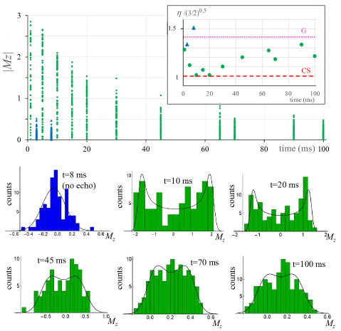
Figure 2: Measurement of the distribution of the normalized magnetization $M_{z}$ following a Ramsey sequence. Each time corresponds to 60 to 100 realizations. Top: Absolute values of $M_{z}$ are plotted for different spin dynamics durations; blue triangles and green circles correspond to experiments without and with spin echo respectively. Inset: The parameter $\eta$ (see text) is evaluated from the corresponding $M_{z}$ distributions. The horizontal lines show the expected value for respectively the PD of a classical spin (dashed, red), and the Gaussian PD (dotted, purple). Bottom: Histograms of the $M_{z}$ distributions are shown together with the PD used to fit them (solid line); see text.

In addition to $\hat{H}_{\rm dd}$, atoms experience a tensor light shift $\hat{H}_{Q}=\sum_{i}B_{\rm Q}({\hat{S}}_{i}^{z})^{2}$. For a non interacting gas this leads to a periodic evolution of $\ell$, with a time scale $\tau_{q}=\frac{h}{4|B_{\rm Q}|}\approx 50$ ms to reach zero for typical $|B_{\rm Q}|/h\approx 5$ Hz in our experiment. This one-body term has to be taken into account in simulations. At short time, it leads to a replacement of $V_{\rm{eff}}\rightarrow V_{\rm eff}\sqrt{1+40B_{Q}^{2}/27V_{\rm eff}^{2}}$ in Eq. 2, thus making the decay of $\ell$ even faster.

Furthermore, magnetic field inhomogeneities described by gradients for the Larmor frequency, $\omega_{\rm L,i}=g\mu_{B}/\hbar\left(B_{0}+\vec{b}.\vec{r_{i}}\right)$, lead to another term in the Hamiltonian, ${\hat{H}}_{B}=\sum_{i}\hbar\omega_{\rm L,i}({\hat{S}}_{i}^{z})$, which generates dephasing and leads to a damping of $\ell$. The damping timescale is $\tau_{b}=\frac{h}{2g\mu_{B}bR}\simeq 3$ ms with $R\simeq 5$ $\mu$m the typical size of the sample, which is shorter than $\tau_{\rm dd}$. In order to compensate for this dephasing, we implement a spin-echo technique, in which spins are rotated by $\pi$ in the middle of the dynamics (see Fig. 1).

One question that naturally arises is whether the spin echo changes as well the evolution of the populations $p_{m_{S}}$ of the different spin components. As shown in Fig. 1, the observed spin dynamics is roughly identical with and without the echo, which is confirmed by GDTWA numerical simulations using the experimental gradient of (10.5$\pm 1$) Gauss.m^-1. This behavior is consistent with a short time perturbative analysis, which predicts that magnetic field gradients only enter at quartic order in the population dynamics, i.e. $p_{m_{S}}(t)-p_{m_{S}}(0)\propto\frac{t^{4}}{N_{S}}[15\sum_{i=1}^{N_{S}}(\sum_{j\neq i}^{N_{S}}V_{ij}(\omega_{Li}-\omega_{Lj}))^{2}-27\sum_{i,j\neq i}^{N_{S}}(\omega_{Li}-\omega_{Lj})^{2}V_{ij}^{2}]$ while dipolar effects enter at second order $\propto t^{2}V_{\rm eff}^{2}$  som .

Our raw experimental results for the measurement of the spin length are shown in Fig. 2 (top). Without a spin echo, a fast damping of the magnetization is observed, in a timescale consistent with $\tau_{b}$. There is here a striking difference with our previous measurements in a bulk BEC Lepoutre et al. (2018), where a gap due to spin-dependent interactions prevents the reduction of magnetization. When a spin echo is applied, the raw data show that $\ell$ decays with a significantly longer timescale, compatible with $\tau_{dd}$. Note nevertheless that given that $\hat{H}_{dd}$ does not commute with $\hat{H}_{B}$ the utility of a spin-echo to protect the decay of $\ell$, is parameter and geometry dependent Solaro et al. (2016).

To obtain a quantitative estimate of $\ell$ as a function of time, we have investigated the probability distributions (PD) associated with the data. Figure 2 shows that a mostly Gaussian PD is obtained for experiments without echo. On the contrary, data with spin-echo only show a Gaussian-like shape at long times. At short time PDs of a totally different kind are obtained, with a maximum of the probability for large values of $|M_{z}|$. To account for this observation, we introduce the probability distribution of a classical spin (CS) of norm $\ell$. Such PD is obtained by differentiating the projection $M_{z}=\ell\cos(\phi)$, thus obtaining the number $dN$ of realization of $M_{z}$:

$$\frac{dN}{dM_{z}}_{CS}=\frac{1}{\pi l}\frac{1}{\sqrt{1-\frac{M_{z}^{2}}{l^{2}}}}$$ (3)

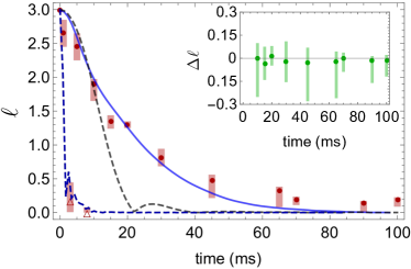
Figure 3: Values of the spin length $\ell$ derived by fitting the distributions of the magnetization $M_{z}$ after the Ramsey sequence. Error bars represent the 68 $\%$ confidence interval, and are detailed in som . Filled circles and empty triangles are measurements with and without the spin echo pulse, respectively. The black dashed line shows the numerical results with the spin echo pulse applied, obtained with GDTWA for the same lattice configuration as in Fig. 1. The blue dashed line shows the dynamics without the spin echo, obtained from the gaussian TWA simulations som . The blue solid line corresponds to GDTWA simulations effectively accounting for atomic motion in the lattice, with $B_{Q}/h=-2$Hz. Inset: difference between the two experimental determinations of $\ell$, comparing the results of the fit of the experimental probability distributions to Eq. (5). Error bars correspond to the quadratic average of the standard deviations associated with either methods.

In order to characterize the observed PDs, we evaluate from the data the square-root of the kurtosis $\eta=\frac{\sqrt{M_{4}}}{M_{2}}$ with $M_{n}=\int PD(x)x^{n}dx$: $\eta=\sqrt{\frac{3}{2}}$ for the PD of eq.(3), and $\eta=\sqrt{3}$ for a Gaussian PD, $\frac{dN}{dM_{z}}_{G}=\frac{1}{\sqrt{\pi}\sigma}\exp\left(-\frac{M_{z}^{2}}{\sigma^{2}}\right)$. The experimental values of $\eta$ are shown in Fig. 2 . Data without echo show a good agreement with a Gaussian PD. For data with a spin-echo, the value of $\eta$ is in good agreement with the classical value for $t_{f}\simeq 5-30$ ms, and it gradually approaches a gaussian value for $t>60$ ms. This first qualitative analysis shows trends for the measured PDs. In order to get numerical values of $\ell$ we have used a convolution of the two PDs described above to fit the data, as shown in Fig. 2; this method assumes that a total dephasing has occurred, which requires $t\geq 10$ ms in our experiment (for $t=1,5$ ms we use another analysis, see som ).

The corresponding results of $\ell$ for each time $t$ are shown in Fig.  3. As expected, without applying the echo pulse $\ell$ decays rapidly; the actual damping rate depends on the system size and lattice geometry. On the other hand, the measured data of $\ell$ after applying the echo pulse reveal an exponential damping of the collective spin towards a small but not zero value, $\ell(t)\simeq(3-\ell_{0})\exp(-t/\tau_{e})+\ell_{0}$, with $\ell_{0}=0.15$ and $\tau_{e}=22$ ms. This contrasts with the glassy dynamics observed in $e.g.$ Signoles et al. (2019).

In order to model the dynamics of $\ell$ in the absence of the echo pulse, it is crucial to appropriately account for the actual sample geometry in experiment and to capture the effects of inhomogeneities. For this purpose, we implement a gaussian TWA approach in our numerical calculation (blue dashed line in Fig. 3) som , which allows for efficiently simulating systems with $N_{s}\sim 10^{4}$, much larger than the size previously investigated Lepoutre et al. (2019). When the echo pulse is applied, we first use GDTWA simulations using the same parameters as those used in Fig. 1. We explicitly insert a $\pi$ rotation around the $y$ axis at half of the evolution time som . While the GDTWA captures the populations dynamics at all times (see Fig. 1), it is only able to reproduce the spin length measurements at $t\leq 10$ ms (black dashed line in Fig. 3). Interestingly, the spin length dynamically evolves for $t>30$ ms whereas the population dynamics and pure spin model numerical simulations have then essentially reached a plateau. This indicates that measuring the collective spin length constitutes a more sensitive probe than simply monitoring spin dynamics.

While tunneling in the lowest band (where atoms are initially loaded) is too slow to explain the discrepancy between the spin-length data and the GDTWA simulations, one possibility could be that phase noise in the lattice could promote particles to higher bands, where tunneling is non-negligible. This type of heating processes was for example also reported with KRb molecules Chotia et al. (2012). To model this possible scenario we performed numerical simulations assuming frozen atoms but relaxing the requirement to be pinned in the regular grid imposed by the lattice potential while keeping the same average density som . This emulates the idea that during a tunneling process on average an atom can be in between two adjacent lattice sites. The calculated dynamics of spin population resulting from this toy model is consistent with the experimental measurements som . The result for $\ell$ is shown with a solid line in Fig. 3: the agreement with the experimental data is much better than the one obtained with GDTWA (black dashed line); however, our toy model predicts a zero relaxation value of the spin length within the experimental time range investigated, in contrast with the experimental observations.

In order to confirm our measurements of $\ell$, we performed a noise analysis of the components of the collective spin. Whether we apply the final $\pi/2$ pulse (Ramsey experiment, labelled R) or not (experiment labelled noR), we measure $\hat{j}_{x}$, or $\hat{j}_{z}$. Taking into account the randomness of $\phi$ Lücke et al. (2014) and a technical noise on the measurements, one obtains the following expressions for the variance of $M_{z}$ when averaging over many realizations:

$$\rm{Var}(M_{z})_{\rm{R}} = \frac{\ell^{2}}{2}+\frac{\rm{Var}(\hat{j}_{X})+\rm{Var}(\hat{j}_{Y})}{2}+\sigma_{\rm{exp}}^{2}\equiv\left<j_{x}^{2}\right>_{\rm{exp}}$$

$$\rm{Var}(M_{z})_{\rm{noR}} = \frac{3}{2N_{s}}+\sigma_{\rm{exp}}^{2}\equiv\left<j_{z}^{2}\right>_{\rm{exp}}$$ (4)

To derive Eq.(4) we add a technical noise (with an associated standard deviation $\sigma_{\rm{exp}}$) to the theoretical expectations. Since our main source of technical noise corresponds to an insufficient signal to noise ratio in the absorption images, measurements of $\hat{j}_{z}$ and $\hat{j}_{x}$ are affected by the same technical noise. Since $\left[\hat{H}_{\rm dd},\hat{J}_{z}\right]=0$, the theoretically expected $\left<\hat{j}_{z}^{2}\right>$ remains equal to its value at $t=0$, i.e. to the standard quantum noise (SQN) $\frac{3}{2N_{s}}$.

Therefore measurements of standard deviations without Ramsey pulse ($\sqrt{\left<j_{z}^{2}\right>_{\rm{exp}}}$) brings a benchmark of the technical noise: our data show that we obtain about $3$ times the SQN for $t=0$, and that the ratio to SQN increases as a function of time som . We therefore can consider that $\left<j_{z}^{2}\right>_{\rm{exp}}\simeq\sigma_{\rm{exp}}^{2}$. The technical noise can be compared with the values predicted by our simulations for the quantum noise of $\hat{j}_{x}$ som : we get $\sigma_{\rm{exp,min}}^{2}>4\times\frac{\rm{Var}(\hat{j}_{X})+\rm{Var}(\hat{j}_{Y})}{2}_{\rm{max}}\simeq\frac{32}{N_{s}}$. We therefore assume that $\left<j_{x}^{2}\right>_{\rm{exp}}\simeq\frac{\ell^{2}}{2}+\sigma_{\rm{exp}}^{2}$, so that:

$$\left<j_{x}^{2}\right>_{\rm{exp}}\simeq\frac{\ell^{2}}{2}+\left<j_{z}^{2}\right>_{\rm{exp}}$$ (5)

Therefore, a signature of a non-zero $\ell$ is that $\left<j_{x}^{2}\right>_{\rm{exp}}$ is larger than the technical noise. This provides a simple measurement of $\ell$ complementary to the method described above, provided that a complete dephasing happens (for $t\geq 10$ ms in our case). The two methods are in good agreement, as shown in the inset of Fig. 3 .

In conclusion, our experiment demonstrates the remarkably different effects of a spin echo on the dynamics of a strongly interacting quantum system for spin population and spin magnetization. Notably, our measurements show that the decay of the transverse magnetization in our experiment is slower than expected, and approaches a small but finite value at long times. This surprising observation indicates that our experiment cannot be fully described by a spin model of frozen particles, a finding that could not be previously deduced from the measurements on population dynamics. This illustrates how measurements of spin coherences provide valuable information on quantum many-body systems that are crucial to benchmarking experiments as quantum simulators. Our work also paves a way towards further investigations using spin coherences to probe quantum many-body phenomena in $S>1/2$ dipolar systems.

I Supplemental Material

I.1 Extensive data: Standard deviations

We show in Fig 4 standard deviations normalized to the standard quantum limit (SQL) $\sqrt{\frac{3}{2N}}$. The experimental values $(\left<j_{x}^{2}\right>_{\rm{exp}}^{1/2}$ normalized to SQL are plotted for all times where total dephasing has occurred (see below). We plot as well our measured values of $(\left<j_{z}^{2}\right>_{\rm{exp}}^{1/2}$ normalized to SQL. During the data taking, we could minimize the technical noise by optimizing the intensity of the probe laser used for absorption imaging; this optimized intensity was used for data at long times, $t=70,90,100$ ms. For these three values of $t$ we measured both $j_{x}$ and $j_{z}$; we measured as well $j_{z}$ for $t=0$ ms, which corresponds to our minimal noise value, but still larger than SQL. We plot as well the normalized standard deviation obtained by our convolution fit analysis (which is the parameter $\sigma_{G}$ below); the good agreement between this standard deviation and the experimental one of $j_{z}$ shows the consistency of our analysis. Data corresponding to $10\leq t\leq 65$ ms are affected by a larger technical noise, hence the discontinuity appearing between $t=65$ and $t=70$ ms.

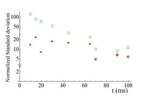
Figure 4: Normalized standard deviations to the standard quantum limit: experimental values for $j_{x}$ (open squares) and $j_{z}$ (open circles); and standard deviation $\sigma_{G}$ of the Gaussian derived from the convolution fit of the $M_{z}$ histograms (full diamonds).

I.2 Estimate of $\ell$ at short time and extended data

As explained in the main article, measurements of $\ell$ are based on two methods, which both require that a full dephasing has occurred, $i.e.$ that the angle $\phi$ between $\mathbf{j}$ and $\hat{x}$ (see main article) uniformly spans $\left[-\pi,+\pi\right]$. For data at short time dephasing has not taken place yet, which leads to non symmetric histograms (for $t=1$ ms and $t=5$ ms).

We show in Fig 5 some additional histograms of the $M_{z}$ distributions not shown in the main article, with the PD used to fit them when it is relevant: as explained above for $t=1$ ms and $t=5$ ms non total dephasing prevents to fit the data.

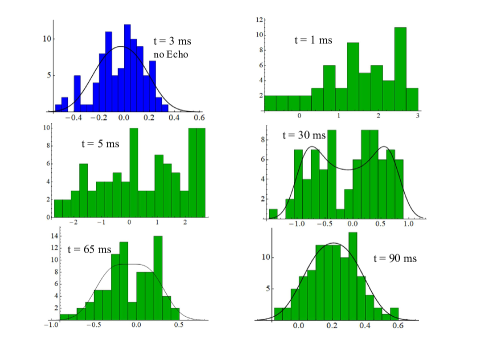
Figure 5: Additional histograms of the $M_{z}$ distributions not shown in the main article, with the PD used to fit them when they are relevant.

We explain here how we evaluate the value of $\ell$ for these two short time values. We assume a classical spin, with a random dephasing angle $\phi$ ranging in the interval $-\frac{\Delta_{\phi}}{2}<\phi<\frac{\Delta_{\phi}}{2}$. Assuming a uniform distribution within this interval, we generate ensembles of values of $\ell\cos(\phi)$ with $N_{\rm{exp}}$ terms, where $N_{\rm{exp}}$ is the number of values of $M_{z}$ in the experimental data. We then look for the value of $\Delta_{\phi}$ and $\ell$ which lead to the same mean value and standard deviation as the ones of the experimental data: this provides our estimate of the central value of $\ell$, $\ell_{c}$. To roughly estimate the error bars, we assume $2\ell_{c}-M_{z\rm{max}}\leq\ell\leq M_{z\rm{max}}$, with $M_{z\rm{max}}$ the maximal experimental value of $M_{z}$: this very likely overestimates the error bar, as for all values of $t\geq 10$ ms the value of $M_{z\rm{max}}$ is beyond error bars on $\ell$. We obtain in addition an estimate of the way the dephasing $\Delta_{\phi}$ grows in the experiment (see Fig 6).

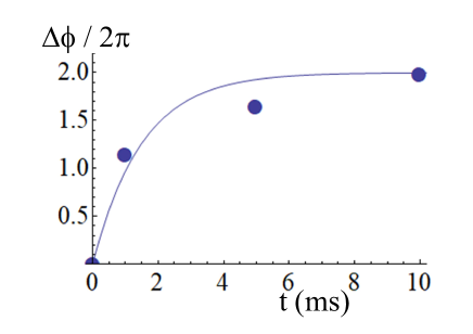
Figure 6: Estimate of the growth of the dephasing $\Delta_{\phi}$ with time in the experiment. The full line is an exponential to guide the eye.

I.3 Error bars on $\ell$

We now describe the way error bars are evaluated for data at $t\geq 10$ ms, when full dephasing has occurred. As explained in the main text, we estimate $\ell$ from two methods.

We start with the method using fit of the experimental Probability Distributions (PDs). We search for the PD which has the same second and fourth moments as the experimental data; these are denoted respectively by $M_{2,\rm{exp}}$ and $M_{4,\rm{exp}}$. This distribution results from a convolution of a Gaussian (characterized by its standard deviation $\sigma_{G}$) and a Classical Spin distribution (characterized by the spin length $\ell_{0}$). The central value of $\ell$ is given by $\ell_{0}$. We use 50 $\%$ sub-sampling of the experimental data to estimate uncertainties on $M_{2,\rm{exp}}$ and $M_{4,\rm{exp}}$. We then vary the values of $M_{2}$ and $M_{4}$ in the intervals provided by the sub-sampling analysis, and obtain from convoluted PDs our estimate of $\ell_{min}$ and $\ell_{max}$, respectively the minimal and maximal value of $\ell$. We assume that the interval $[\ell_{min};\ell_{max}]$ defines the two-standard-deviations confidence interval for $\ell$.

We also performed the following analysis to better ascertain the non-zero value of $\ell$ at long times. For that we generate numerically large number of samples with a Gaussian statistics, with the same number of values of $M_{z}$ (noted $N_{exp}$), the same mean value and standard deviation $\sqrt{M_{2}}$ as the ones of the experimental sample. We then obtain a list of values of the parameter $\eta=\frac{\sqrt{M_{4}}}{M_{2}}$ (see main text) with a mean value close to $\sqrt{3}$, and a standard deviation $\sigma_{eta}$. It gives us an estimate of the probability that the experimental sample is compatible with a pure Gaussian PD. For example at $t=70$ ms, we obtain $\eta_{exp}=1.45$ for the experimental $M_{z}$ data, and $\sigma_{eta}=0.12$ ($N_{exp}=106$). Using this analysis, the probability that the experimental PD is compatible with a pure Gaussian is given by $\int_{-\infty}^{-(\sqrt{3}-\eta_{exp})/\sigma_{\eta}}\frac{1}{\sqrt{(}\pi)}\exp(-x^{2})dx=0.01$. We find this probability to be $0.27$ for $t=90$ ms, and $0.03$ for $t=100$ ms. Since a Gaussian distribution is necessarily obtained for $\ell=0$ (assuming a negligible quantum noise), our analysis can exclude $\ell=0$ with a very high confidence for $t=70,100$ ms (while $\ell=0$ cannot be fully excluded at 90 ms).

We now turn to the determination of $\ell$ by the second method described in the article, see eq.(5). For $t=70,90,100$ ms we simply apply the formula with measured values of $\left<j_{x}^{2}\right>_{\rm{exp}}$ and $\left<j_{z}^{2}\right>_{\rm{exp}}$ (see Fig 4). For $5\leq t\leq 65$, we take for $\left<j_{z}^{2}\right>_{\rm{exp}}$ the variance of the data with no echo at $t=8$ ms: the corresponding probability distribution being very close to a Gaussian, we assume that its variance corresponds to the technical noise. As for error bars for this second method, uncertainties on $\left<j_{x}^{2}\right>_{\rm{exp}}$ and $\left<j_{z}^{2}\right>_{\rm{exp}}$ are evaluated through sub-sampling, which yields standard deviation on these quantities to be about $5\%$.

I.4 Theoretical model

We describe the experimental system with the Hamiltonian

$$\hat{H}=\sum_{\bf r}B({\bf r})\hat{S}^{z}_{\bf r}+B_{Q}\sum_{\bf r}(\hat{S}^{z}_{\bf r})^{2}$$

$$+\frac{V({\bf r},{\bf r}^{\prime})}{2}\sum_{{\bf r}\neq{\bf r}^{\prime}}[\hat{S}^{z}_{\bf r}\hat{S}^{z}_{{\bf r}^{\prime}}-\frac{1}{2}(\hat{S}^{x}_{\bf r}\hat{S}^{x}_{{\bf r}^{\prime}}+\hat{S}^{y}_{\bf r}\hat{S}^{y}_{{\bf r}^{\prime}})]$$ (6)

where ${\bf r}$ denotes the coordinates of the lattice sites, and $\hat{S}^{x,y,z}_{\bf r}$ are spin-3 angular momentum operators acting on atoms located at ${\bf r}$ . For atoms frozen at discrete lattice sites, ${\bf r}=i_{x}d_{x}\hat{x}+i_{y}d_{y}\hat{y}+i_{z}d_{z}\hat{z}$ for the ${\bf i}$th atom. Here $d_{x,y,z}$ are lattice constants along the different directions. $V({\bf r},{\bf r}^{\prime})$ denotes the dipolar interactions between two atoms located at ${\bf r}$ and ${\bf r}^{\prime}$, and its explicit form is given in the main text between arbitrary ${\bf i}$ and ${\bf j}$ atoms. $B(\bf r)={\bf b}\cdot{\bf r}$ accounts for the inhomogeneous magnetic fields in the experiment.

To obtain the spin dynamics accounting for actual experimental conditions, we utilized the GDTWA approach introduced in Ref. Zhu et al. (2019) to numerically solve the time evolution under Eq. (6). For the case where an echo pulse is applied, we first numerically evolve the system under $\hat{H}$ for $t/2$, then implement a $\pi$ rotation around the $y$ axis, and evolve the system under $\hat{H}$ for another $t/2$ afterwards, to find the resulting dynamics at time $t$. Namely, the whole time evolution operator is $\hat{\mathcal{U}}_{\rm echo}(t,0)=e^{-i\hat{H}t/2\hbar}e^{-i\pi\hat{S}^{y}}e^{-i\hat{H}t/2\hbar}$, with $\hat{S}^{y}=\sum_{\bf r}\hat{S}_{\bf r}^{y}$. In Fig. 1 of the main text, we first simulated the population dynamics of the different spin components $p_{m_{s}}(t)$ for a unit-filled lattice with $(L_{x},L_{y},L_{z})$ number of sites along $(x,y,z)$ directions, using experimental values of $d_{x,y,z}$ and ${\bf b}$, for both the cases with and without a spin echo pulse. Since $d_{y}\approx 2d_{z}\approx 2d_{x}$, we used $(L_{x},L_{y},L_{z})=(14,7,14)$ in our calculation. The resulting dynamics shows a convergence for such system sizes. Since $B_{Q}$ is not exactly known in experiment, it was chosen as a fitting parameter bounded by experimental estimation of $|B_{Q}|/h\leq 6$Hz. It was held fixed when comparing the echo and no echo cases. We find a good agreement between the numerics and experimental data, with small differences between the two cases.

As mentioned in the main text, a useful way to understand this behavior is to examine the short-time quantum dynamics. Utilizing the series expansion of the evolution operator $\hat{\mathcal{U}}=e^{-i\hat{H}t}=\sum_{k}\frac{(-i)^{k}t^{k}}{k!}\hat{H}^{k}$, we can express $p_{ms}(t)$ in different powers of $t$. We find that even without the echo pulse, the leading contribution to the population change $\delta(p_{ms})=p_{ms}(t)-p_{ms}(0)$ comes from interactions. To provide an explicit description of the dynamics, here we focus on the change for $m_{s}=0$, for which the leading contribution is

$$\delta(p_{0}) \propto-\frac{135t^{2}}{128}V_{\rm eff}^{2}$$ (7)

and is not affected by the inhomogeneity ${\bf b}$. The effect of ${\bf b}$ shows up in the dynamics at later time as

$$\delta(p_{0})=\Gamma\frac{5t^{4}}{256N}$$ (8)

with $\Gamma=15\sum_{{\bf r}}[\sum_{{\bf r}^{\prime}\neq{\bf r}}V({\bf r},{\bf r}^{\prime})({\bf b}\cdot({\bf r}-{\bf r}^{\prime})]^{2}-27\sum_{{\bf r},{\bf r}^{\prime}\neq{\bf r}}({\bf b}\cdot({\bf r}-{\bf r}^{\prime}))^{2}V({\bf r},{\bf r}^{\prime})^{2}$. Similar effects also apply to other $m_{s}$ states and we refer the interested readers to Ref. Lepoutre et al. (2019) for relevant details. In contrast, the dynamics of $\ell$ is much more sensitive to the echo pulse and the lattice configuration.

When a spin echo pulse is absent, the dynamics of $\ell$ is dominated by single-particle processes and depends on the lattice configuration and atomic density distribution. For a lattice fully filled with atoms frozen at discrete lattice sites, it can be described as:

$$\frac{\ell(t)}{24}=\frac{\cos^{5}(B_{Q}t/\hbar)}{\gamma_{x}\gamma_{y}\gamma_{z}t^{3}}|\sin(\frac{\gamma_{x}t}{2})\sin(\frac{\gamma_{y}t}{2})\sin(\frac{\gamma_{z}t}{2})|$$ (9)

where $\gamma_{x,y,z}=b_{x,y,z}L_{x,y,z}/\hbar$. It is straightforward to estimate from Eq. (9) that under typical experimental conditions, $\ell$ already decays significantly within $5$ms. In comparison, when a spin echo pulse is applied, up to second order in time we find

$$\ell(t) = 3-\frac{3t^{2}}{16\hbar^{2}}(40B_{Q}^{2}+27V_{\rm eff}^{2})+O(t^{3})$$ (10)

which shows that the effect of ${\bf b}$ is removed as a result of the echo pulse at second order in $t$. In this case the decay of $\ell$ mainly comes from dipolar interactions and happens at a rate much slower than the one without echo. It is worth to note that while for Ising interactions, such as those between dressed Rydberg atoms Mukherjee et al. (2016), spin echo technique can completely cancel the effect of inhomogneous field ${\bf b}$, for dipolar interactions, there is a small residual effect due to the noncommutativity between different terms in Eq. (6), which can show up at longer times.

Since as indicated by Eq. (9) the dynamics of $\ell$ without a spin echo strongly depends on the lattice size, in the numerical calculation, we use a large lattice that is closer to real experimental conditions, where atoms populate a shell of outer radius $r_{\rm out}\approx 23d$ and inner radius $r_{\rm in}\approx 18d$, with $d=266$nm the smallest lattice spacing Lepoutre et al. (2019). At unit-filling, this volume includes $N\approx 10^{4}$ atoms, which is much larger than the system size investigated before Lepoutre et al. (2019). Although the quantum many-body dynamics for such a large system can still be simulated with our GDTWA approach, we find an alternative approach can significantly reduce the computational cost while capturing the collective spin dynamics in this case. In the alternative approach, we use a Gaussian sampling of three spin-variables $\sum_{\bf r}\langle\hat{S}^{x,y,z}_{\bf r}\rangle$ which neglects intra-spin correlations as described in Ref. Zhu et al. (2019). While this approach does not correctly account for the effect of $B_{Q}$, for this case without the echo pulse the effect of $B_{Q}$ is much weaker compared to the effect of inhomogeneities, and the time evolution of $\ell$ can nevertheless be well captured. The result is plotted in Fig. 3 by the blue dashed line, which agrees well with experimental data. We note that throughout this work, the gaussian TWA approach is only used for solving the time evolution of $\ell$ in the absence of an echo pulse, while all other simulations are performed with GDTWA.

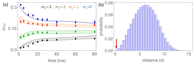
Figure 7: (a) Dynamics of spin population calculated with GDTWA (lines) using the same model and parameters as for the blue solid line in Fig. 3. Different colors represent dynamics for different spin components: $m_{s}=-3$, $m_{s}=-2$, $m_{s}=-1$, $m_{s}=0$ from bottom to top. Color bands account for imperfection in the first pulse as in Fig. 1. (b) Distribution of inter-particle spacing in the GDTWA simulation, in the units of $d$. The leftmost bin (indicated by the red arrow) shows the fraction of atoms with distance closer than $r_{\rm cutoff}$, which is very small. Practically, in the GDTWA simulation all distances smaller than $r_{\rm cutoff}$ are set to be equal to $r_{\rm cutoff}$. This is partially motivated by the intuition that the contact interaction between Cr atoms under the experimental condition is very strong ($\sim$kHz Fersterer et al. (2019)) and thus prevents two atoms from being very close. Besides, since this fraction is tiny, except for small differences on the short-time scale ($\sim\hbar/18V_{0}\sim 5$ms, where $V_{0}=\frac{\mu_{0}(g\mu_{B})^{2}}{4\pi d^{3}}$), the overall dynamics should remain similar for different choices of $r_{\rm cutoff}\leq d$. The atom number used in the simulation is $N=200$, which gives an overall density of $N/(L_{x}L_{y}L_{z})\approx 0.6$.

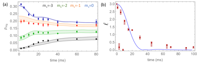
Figure 8: Dynamics of spin population (a) and spin length (b) calculated with GDTWA (lines) for a regular lattice similar to the one in Fig. 1 (c) but with nonunity filling. To compare with the model accounting for atomic motion, the filling fraction is chosen to be $60\%$, close to the density used in Fig. 7. Lines in (a) plot dynamics for $m_{s}=-3$, $m_{s}=-2$, $m_{s}=-1$, $m_{s}=0$ from bottom to top. Color bands account for imperfection in the first pulse as in Fig. 1. A value $B_{Q}/h=-3$Hz is used for best describing the experimental spin dynamics $p_{m_{s}}$.

For the case with an echo pulse applied, the spin dynamics is insensitive to the magnetic field gradients and thus does not strongly depend on the lattice size when the filling is unity. However, the theoretically calculated dynamics only captures the short-time dynamics well while shows significantly faster decay than experimental measurement at longer times [Fig. 3 black dashed line], where heating and tunneling effects becomes important. Although there is not an efficient way to exactly solve the quantum dynamics fully accounting for these effects and for sufficiently large system size, we investigate the spin dynamics including these effects in a phenomenological way. Instead of using a spin model where all atoms are frozen at discrete lattice sites, we allow a continuous random uniform distribution of ${\bf r}$ in a lattice of size $(L_{x},L_{y},L_{z})$, while keeping atoms at least $r_{\rm cutoff}=0.5d$ away from each other [see Fig. 7 caption]. Both the evolution of spin population [Fig7(a)] and $\ell$ [solid line in Fig. 3] obtained with this model capture well the experimental observations.

The spin dynamics can slow down due to non-unit filling of the lattice, which also introduces disorder in the spin couplings, as was the case in Ref. Yan et al. (2013). In our experiment numerical simulations performed at lower filling fractions with frozen particles indicate lower filling is not the cause of the observed slower contrast dynamics in the experiment. To further illustrate this, in Fig. 8 we calculate the spin dynamics for a partially filled lattice, with atoms frozen at discrete sites. While the spin population evolves in a similar way as in Fig. 7 and still describes experimental data, the calculated $\ell(t)$ significantly deviates from the experimental dynamics.

In Fig. 9, we plot the numerically calculated probability distribution of the normalized magnetization for the toy model that accounts for heating and tunneling by allowing particles to be at continuous locations within the array. Our theoretical model also well describe the measured probability distributions (see FiG. 2 main text).

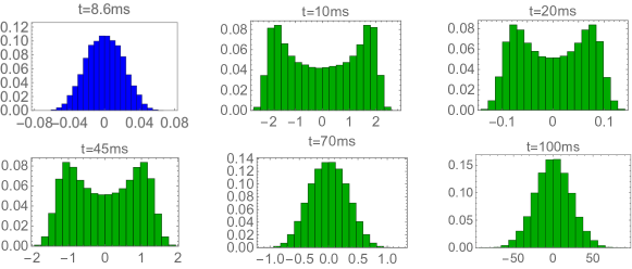
Figure 9: Probability distributions of the normalized magnetization for the cases without (blue) and with (green) an echo pulse, obtained with the model and parameters used in Fig. 3 for the blue dashed and solid lines, respectively.

To further provide information on the quantum noise generated by strong interactions during the time evolution, in Fig. 10, we use GDTWA to calculate the variance of collective spin projections, ${\rm Var({\hat{j}}_{X})}$ for a unit-filled lattice, as used for Fig. 1(c).

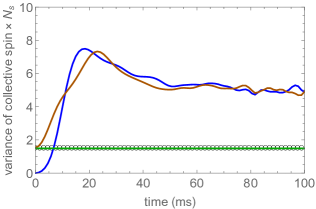
Figure 10: Variance of collective spin projections, ${\rm Var({\hat{j}}_{X})}$ (blue solid line), ${\rm Var({\hat{j}}_{Y})}$ (brown solid line), and ${\rm Var({\hat{j}}_{z})}$ (green solid line), each multiplied by $N_{s}$. The results are obtained from GDTWA simulations for a unit-filled lattice with the same geometry as for Fig. 1(c), and with $B_{Q}/h=-5$Hz. The empty circles show the standard quantum noise $3/2$ for $S=3$ atoms.