Network-to-Network Translation with
Conditional Invertible Neural Networks

Abstract

Given the ever-increasing computational costs of modern machine learning models, we need to find new ways to reuse such expert models and thus tap into the resources that have been invested in their creation. Recent work suggests that the power of these massive models is captured by the representations they learn. Therefore, we seek a model that can relate between different existing representations and propose to solve this task with a conditionally invertible network. This network demonstrates its capability by (i) providing generic transfer between diverse domains, (ii) enabling controlled content synthesis by allowing modification in other domains, and (iii) facilitating diagnosis of existing representations by translating them into interpretable domains such as images. Our domain transfer network can translate between fixed representations without having to learn or finetune them. This allows users to utilize various existing domain-specific expert models from the literature that had been trained with extensive computational resources. Experiments on diverse conditional image synthesis tasks, competitive image modification results and experiments on image-to-image and text-to-image generation demonstrate the generic applicability of our approach. For example, we translate between BERT and BigGAN, state-of-the-art text and image models to provide text-to-image generation, which neither of both experts can perform on their own.

1 Introduction

One of the key features of intelligence is the ability to combine and transfer information between diverse domains and modalities [12, 73, 65, 68, 61]. In contrast, artificial intelligence research has made great progress in learning powerful representations for individual domains [28, 71, 19, 69, 15, 5] that can even achieve superhuman performance on confined tasks such as traffic sign recognition [10, 11], image classification [29] or question answering [15]. However, learning representations for different domains that also allow a domain-to-domain transfer of information between them is significantly more challenging [2]: There is a trade-off between the expressiveness of individual domain representations and their compatibility to another to support transfer. While for limited training data multimodal learning has successfully trained representations for different domains together [66, 74], the overall most powerful domain-specific representations typically result from training huge models specifically for individual challenging domains using massive amounts of training data and computational resources, e.g. [19, 69, 5].

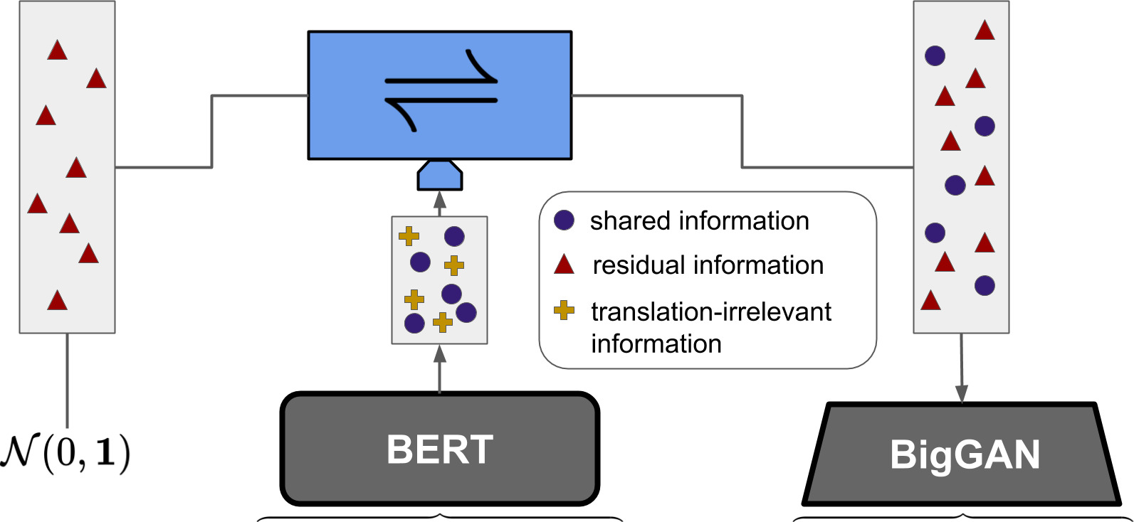
			source domain	target domain
			A blue bird sitting on top of a field
			A yellow bird is perched on a branch
A park bench sitting in the middle of a park			A couple of zebras are standing in a field
A pizza sitting on top of a white plate			A school bus parked in a parking lot

Figure 1: BERT [15] to BigGAN [4] transfer: Our approach enables translation between fixed off-the-shelve expert models such as BERT and BigGAN without having to modify or finetune them.

With the dawn of even more massive models like the recently introduced GPT-3 [5], where training on only a single domain already demands most of the available resources, we must find new, creative ways to make use of these powerful models, which none but the largest institutions can afford to train and experiment with, and thereby utilize the huge amount of resources and knowledge which are distilled into the model’s representations—in other words, we have to find ways to cope with "The Bitter Lesson" [67].

Consequently, we seek a model for generic domain-to-domain transfer between arbitrary fixed representations that come from highly complex, off-the-shelf, state-of-the-art models and we learn a domain translation that does not alter or retrain the individual representations but retains the full capabilities of original expert models. This stands in contrast to current influential domain transfer approaches [41, 51, 83] that require learning or finetuning existing domain representations to facilitate transfer between them.

Since different domains are typically not isomorphic to another, i.e. translations between them are not uniquely determined, the domain translation between fixed domain representations requires learning the corresponding ambiguities. For example, there are many images which correspond to the same textual description and vice versa. To faithfully translate between domains, we employ a conditional invertible neural network (cINN) that also explicitly captures these transfer uncertainties. The INN conditionally learns a unique translation of one domain representation together with its complementary residual onto another. This generic network-to-network translation between arbitrary models can efficiently transfer between diverse state-of-the-art models such as transformer-based natural language model BERT [15] and a BigGAN [4] for image synthesis to achieve competitive text-to-image translation, see Fig. 1.

To summarize, our contributions are as follows: We (i) provide a generic approach that allows to translate between fixed off-the-shelf model representations, (ii) learns the inherent ambiguity of the domain translation, which facilitates content creation and model diagnostics, and (iii) enables compelling performance on various different domain transfer problems. We (iv) make transfer between domains and datasets computationally affordable, since our method does not require any gradient computations on the expert models but can directly utilize existing representations.

2 Related Work

The majority of approaches for deep-learning-based domain-to-domain translation are based on generative models and therefore rely on Variational Autoencoders (VAEs) [37, 58], Generative Adversarial Networks (GANs) [27], autoregressive models [70], or normalizing flows [50] obtained with invertible neural networks (INNs) [16, 17]. Generative models transform samples from a simple base distribution, mainly a standard normal or a uniform distribution, to a complex target distribution, e.g. the distribution of (a subset of) natural images.

Sampling the base distribution then leads to the generation of novel content. Recent works [76, 22] also utilize INNs to transform the latent distribution of an autoencoder to the base distribution. A simple structure of the base distribution allows rudimentary control over the generative process in the form of vector arithmetic applied to samples [53, 56, 62, 26], but more generally, providing control over the generated content is formulated as conditional image synthesis. In its most basic form, conditional image synthesis is achieved by generative models which, in addition to a sample from the base distribution, take class labels [47, 36] or attributes [30] into account. More complex conditioning information are considered in [82, 55], where textual descriptions provide more fine-grained control over the generative process. A wide range of approaches can be characterized as image-to-image translations where both the generated content and the conditioning information is given by images. Examples for conditioning images include grayscale images [84], low resolution images [38], edge images [33], segmentation maps [51, 7] or heatmaps of keypoints [23, 43]. Many of these approaches build upon [33], which introduced a unified approach for image-to-image translation. We take this unification one step further and provide an approach for a wide range of conditional content creation, including class labels, attributes, text and images as conditioning. In the case of image conditioning, our approach can be trained either with aligned image pairs as in [33, 7, 51] or with unaligned image pairs as in [87, 39, 9, 32, 21].

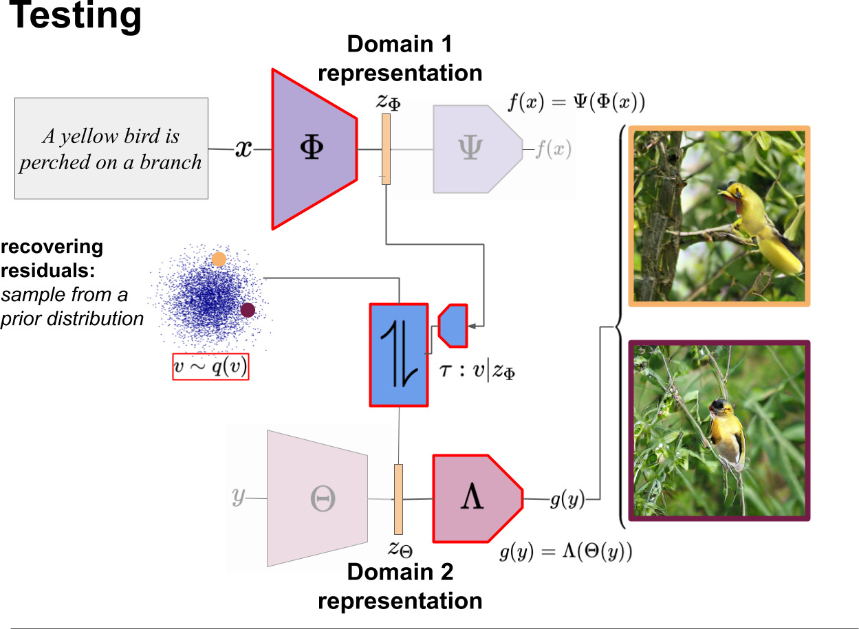
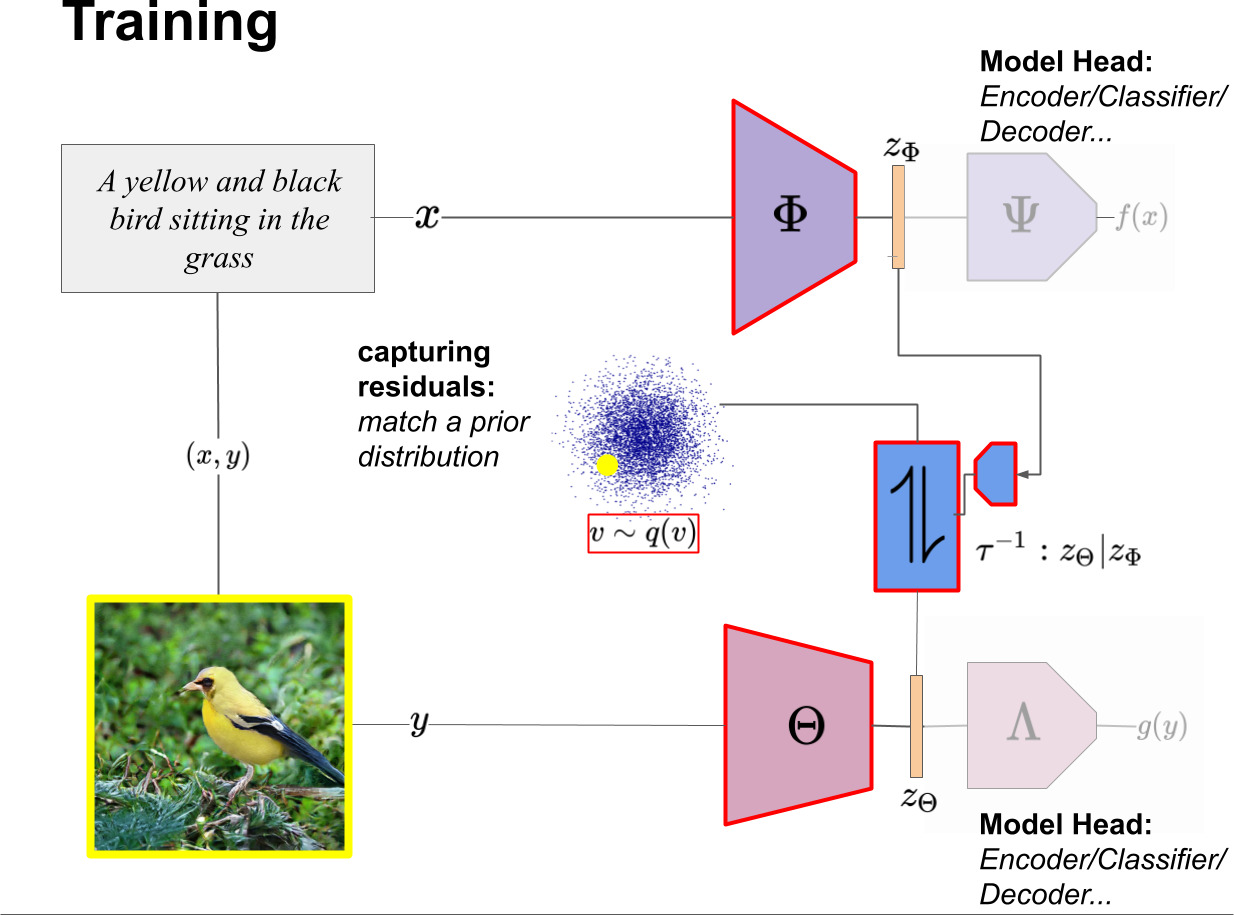
Figure 2: Proposed architecture. We provide post-hoc model fusion for two given deep networks $f=\Phi\circ\Psi$ and $g=\Theta\circ\Lambda$ which live on arbitrary domains $\mathcal{D}_{x}$ and $\mathcal{D}_{y}$. For deep representations $z_{\Phi}=\Phi(x)$ and $z_{\Theta}=\Theta(y)$, a conditional INN $\tau$ learns to transfer between them by modelling the ambiguities w.r.t. the translation as an explicit residual, enabling transfer between given off-the-shelf models and their respective domains.

While many works on generative models focus on relatively simple datasets containing little variations, e.g. CelebA [42] containing only aligned images of faces, [4, 19] demonstrated the possibility to apply these models to large-scale datasets such as ImageNet [14]. However, such experiments require a computational effort which is typically far out of reach for individuals. Moreover, the need to retrain large models for experimentation hinders rapid prototyping of new ideas and thus slows down progress. Making use of pre-trained neural networks can significantly reduce the computational budget and training time. For discriminative tasks, the ability to effectively reuse pre-trained neural networks has long been recognized [54, 18, 80]. For generative tasks, however, there are less works that aim to reuse pre-trained networks efficiently. Features obtained from pre-trained classifier networks are used to derive style and content losses for style transfer algorithms [24], and they have been demonstrated to measure perceptual similarity between images significantly better than pixelwise distances [44, 85]. [81, 45] find images which maximally activate neurons of pre-trained networks and [60] shows that improved synthesis results are obtained with adversarially robust classifiers. Instead of directly searching over images, [49] uses a pre-trained generator network of [20], where it was used to reconstruct images from feature representations. However, these approaches are limited to neuron activation problems, rely on per-example optimization problems, which makes synthesis slow, and do not take into account the probabilistic nature of the conditional synthesis task, where a single conditioning corresponds to multiple outputs. To address this, [48] learns an autoregressive model conditioned on specific layers of pre-trained models and [63] a GAN based decoder conditioned on a feature pyramid of a pre-trained classifier. In contrast, our approach efficiently utilizes pre-trained models, both for conditioning as well as for image-synthesis, such that their combination provides new generative capabilities for content creation through conditional sampling, without requiring the pre-trained models to be aware of these emerging capabilities.

3 Approach

Our goal is to learn relationships and transfer between representations of different domains obtained from off-the-shelf models, see Fig. 2. To be generally applicable to complex state-of-the-art representations, we only assume the availability of already trained models, but no practical access to their training procedure due to their complexity [15] or missing components (e.g. a discriminator, which was not released for [19]). Let $\mathcal{D}_{x}$ and $\mathcal{D}_{y}$ be two domains we want to transfer between. Moreover, $f(x)$ denotes an expert model that has been trained to map $x\in\mathcal{D}_{x}$ onto desired outputs, e.g. class labels in case of classification tasks, or synthesized images for generative image models. To solve its task, a neural network $f$ has learned a latent representation $z_{\Phi}=\Phi(x)$ of domain $\mathcal{D}_{x}$ in some intermediate layer, so that subsequent layers $\Psi$ can then solve the task as $f(x)=\Psi(\Phi(x))$. For $y\in\mathcal{D}_{y}$ let $g(y)=\Lambda(\Theta(y))$ be another, totally different model that provides a feature representation vector $z_{\Theta}=\Theta(y)$.

In general, we cannot expect a translation from $x$ to $y$ to be unique, since two arbitrary domains and their representations are not necessarily isomorphic. For example, a textual description $x$ of an image $y$ usually leaves many details open and the same holds in the opposite direction, since many different textual descriptions are conceivable for the same image by focusing on different aspects. This implies a non-unique mapping from $z_{\Phi}$ to $z_{\Theta}$. Moreover, much of the power of model $f$ trained for a specific task stems from its ability to ignore task-irrelevant properties of $x$. The invariances of $z_{\Phi}$ with respect to $z_{\Theta}$ further increase the ambiguity of the domain translation. Obtaining a plausible $z_{\Theta}$ for a given $z_{\Phi}$ is therefore best described probabilistically as sampling from $p(z_{\Theta}|z_{\Phi})$. Our goal is to model this process with a translation function $\tau$. Thus, we must introduce a residual $v$, such that for a given $z_{\Phi}$, $v$ uniquely determines $z_{\Theta}$ resulting in the translation function $\tau$:

$$z_{\Theta}=\tau(v|z_{\Phi})$$ (1)

Learning a Domain Translation $\tau$:

How can we estimate $v$? $v$ must capture all information of $z_{\Theta}$ not represented in $z_{\Phi}$, but no information that is already represented in $z_{\Phi}$. Hence, to infer $v$, we must take into account both $z_{\Theta}$, to extract information, and $z_{\Phi}$, to discard information. The unique determination of $z_{\Theta}$ from $v$ for a given $z_{\Phi}$ implies the existence of the inverse of $\tau$, when considered as a function of $v$. Thus for every $z_{\Phi}$, the inverse $\tau^{-1}(\cdot|z_{\Phi})$ of $\tau(\cdot|z_{\Phi})$ exists,

$$v=\tau^{-1}(z_{\Theta}|z_{\Phi}).$$ (2)

This structure of $\tau$ is most naturally represented by a conditionally invertible neural network (cINN), for which $\tau^{-1}$ can be explicitly computed, and which we build from affine coupling [17], actnorm [35] and shuffling layers, see Sec. G.1. It then remains to derive a learning task which ensures that information of $z_{\Phi}$ is discarded in $v$. To formalize this goal, we consider training pairs $\{(x,y)\}\subset\mathcal{D}_{x}\times\mathcal{D}_{y}$ and their corresponding features $\{(z_{\Phi},z_{\Theta})\}$ as samples from their joint distribution $p(z_{\Phi},z_{\Theta})$. $v$ can then be considered as a random variable via the process

$$v=\tau^{-1}(z_{\Theta}|z_{\Phi}),\quad\text{with }z_{\Phi},z_{\Theta}\sim p(z_{\Phi},z_{\Theta}).$$ (3)

Then $v$ discards all information of $z_{\Phi}$ if $v$ and $z_{\Phi}$ are independent. To achieve this independence, we minimize the distance between the distribution $p(v|z_{\Phi})$ induced by $\tau$ via Eq.  (3) and some prior distribution $q(v)$. The latter can be chosen arbitrarily as long as it is independent of $z_{\Phi}$, its density can be evaluated and samples can be drawn. In practice we use a standard normal distribution. Using the invertibility of $\tau$, we can then explicitly calculate the Kullback-Leibler divergence between $p(v|z_{\Phi})$ and $q(v)$ averaged over $z_{\Phi}$ (see Sec. B for the derivation):

$$\mathbb{E}_{z_{\Phi}}\operatorname{KL}(p(v|z_{\Phi})|q(v))= \mathbb{E}_{z_{\Theta},z_{\Phi}}\left\{-\log q(\tau^{-1}(z_{\Theta}|z_{\Phi}))-|\det J_{\tau^{-1}}(z_{\Theta}|z_{\Phi})|\right\}-H(z_{\Theta}|z_{\Phi}).$$ (4)

Here, $\det J_{\tau^{-1}}$ denotes the determinant of the Jacobian of $\tau^{-1}$ and $H$ is the (constant) data entropy. If $\tau$ minimizes Eq. (4), we have $p(v|z_{\Phi})=q(v)$, such that the desired independence is achieved. Moreover, we can now simply achieve the original goal of sampling from $p(z_{\Theta}|z_{\Phi})$ by translating from $z_{\Phi}$ to $z_{\Theta}=\tau(v|z_{\Phi})$ with $v$ sampled from $q(v)$, which properly models the inherent ambiguity.

Interpretation as Information Bottleneck:

One of the main goals of minimizing Eq. (4) is the independence of $v$ and $z_{\Phi}$. While it is clear that this independence is achieved by a minimizer, Eq. (4) is also an upper bound on the mutual information $I(v,z_{\Phi})$ between $v$ and $z_{\Phi}$. Thus, its minimization works directly towards the goal of independence. Indeed, following [1], we have

$$I(v,z_{\Phi})=\int_{v,z_{\Phi}}p(v,z_{\Phi})\log\frac{p(v,z_{\Phi})}{p(v)p(z_{\Phi})}=\int_{v,z_{\Phi}}p(v,z_{\Phi})\log p(v|z_{\Phi})-\int_{v}p(v)\log p(v)$$ (5)

Positivity of the KL divergence implies $\int p(v)\log p(v)\geq\int p(v)\log q(v)$, such that

$$I(v,z_{\Phi})\leq\int_{v,z_{\Phi}}p(v,z_{\Phi})\log\frac{p(v|z_{\Phi})}{q(v)}=\mathbb{E}_{z}{}_{\Phi}\operatorname{KL}(p(v|z_{\Phi})|q(v))=\text{Eq.~{}\eqref{eq:loss}}$$ (6)

In contrast to the deep variational information bottleneck [1], our use of a cINN has the advantage that it does not require the hyperparameter $\beta$ to balance the independence of $v$ and $z_{\Phi}$ against their ability to reconstruct $z_{\Theta}$. The cINN guarantees perfect reconstruction abilities of $z_{\Theta}$ due to its invertible architecture and it thus suffices to minimize $I(v,z_{\Phi})$ on its own.

Domain Transfer Between Fixed Models:

At inference time, we obtain translated samples $z_{\Theta}$ for given $z_{\Phi}$ by sampling from the residual space $v$ given $z_{\Phi}$ and then applying $\tau$,

$$z_{\Theta}\sim p(z_{\Theta}|z_{\Phi})\quad\iff\quad v\sim q(v),\;z_{\Theta}=\tau(v|z_{\Phi}).$$ (7)

After training our domain translator, transfer between $\mathcal{D}_{x}$ and $\mathcal{D}_{y}$ is thus achieved by the following steps: (i) sample $x$ from $p(x)$, (ii) encode $x$ into the latent space $z_{\Phi}=\Phi(x)$ of expert model $f$, (iii) sample a residual $v$ from the prior $q(v)$, (iv) conditionally transform $z_{\Theta}=\tau(v|z_{\Phi})$, and (v) decode $z_{\Theta}$ into the domain $\mathcal{D}_{y}$ of the second expert model: $y=\Lambda(z_{\Theta})$.

Note that this approach has multiple advantages: (i) hidden representations usually have lower dimensionality than $x$, which makes transfer between arbitrary complex domains affordable, (ii) the cINN $\tau$ can be trained by minimizing the negative log-likelihood, independent of the domains $\mathcal{D}_{x}$ and $\mathcal{D}_{y}$, and (iii) the approach does not require to take any gradients w.r.t. the expert models $f$ and $g$.

4 Experiments

We investigate the wide applicability of our approach by performing experiments with multiple domains, datasets and models: (1) text-to-image translation by combination of BigGAN and BERT, (2) exploration of the reusability of a fixed autoencoder combined with multiple models including a ResNet-50 classifier and a DeepLabV2 [6] segmentation model for various image-to-image translation tasks and diagnostic insights into the respective models, and (3) comparison to existing methods for image modification and applications in exemplar-guided and unpaired image translation tasks. As our method does not require gradients w.r.t. the models $f$ and $g$, training of the cINN can be conducted on a single Titan X GPU.

Table 1: Inception and FID scores for BERT-to-BigGAN transfer on captions from COCO-stuff. Our approach is on-par with the current state of the art but does not require training of a text-encoder and image-decoder.

	our	SD-GAN [79]	AttnGAN [78]	StackGAN [82]	DM-GAN [88]	MirrorGAN [52]	HDGAN [86]
IS $\uparrow$	$\mathbf{34.7\pm 0.3}$	$\mathbf{35.7\pm 0.5}$	$25.9\pm 0.5$	$8.5\pm 0.1$	$30.5\pm 0.6$	$26.5\pm 0.4$	$11.9\pm 0.2$
FID $\downarrow$	$\mathbf{30.63}$	-	$35.49$	-	$32.64$	-	-

4.1 Translation to BigGAN

This section is dedicated to the task of using a popular but computationally expensive to train expert model as an image generator: BigGAN [4], achieving state-of-the-art FID scores [31] on the ImageNet dataset. As most GAN frameworks in general and BigGAN in particular do not include an explicit encoder into a latent space, we aim to provide an encoding from an arbitrary domain by using an appropriate expert model $f$. Aiming at the reusability of a fixed BigGAN $g$, and given the hidden representation $z_{\Phi}=\Phi(x)$ of the expert model $f=\Psi\circ\Phi$, we want to find a mapping between $z_{\Phi}$ and the latent space $z_{\Theta}$ of BigGAN’s generator $\Lambda$, where, in accordance with Fig. 2, $\Theta\equiv\mathbb{1}$ and $g=\Lambda$. Technical details regarding the training of our cINN can be found in Sec. G.2.

BERT-to-BigGAN Translation:

The emergence of transformer-based networks [72] has led to an immense leap in the field of natural language processing, where a popular model is the so-called BERT model. Here, we make use of a variant of the original model, which modifies BERT such that it produces a latent space in which input sentences can be compared for similarity via the cosine-distance measure [57]. We aim to combine this representational power with the synthesis capabilities of BigGAN and thus train our model $\tau$ to map from the language representations $z_{\Phi}=\Phi(x)$ into the latent space $z_{\Theta}$ of BigGAN’s generator as described above; hence $f=\Phi$ and $\Psi=\mathbb{1}$. During training, access to textual descriptions is obtained by using a captioning model as in [77], trained on the COCO [40] dataset. In a nutshell, at training time, we sample $z_{\Theta}$, produce a corresponding image $\Lambda(z_{\Theta})$, utilize [77] to produce a text-caption $x$ describing the image and subsequently produce a sentence representation $z_{\Phi}=\Phi(x)$ which we use to minimize the overall objective Eq. (4). Results can be found in Fig. 1 and Tab. 1. Our model captures both fine-grained and coarse descriptions (e.g. blue bird vs. yellow bird; school bus vs. pizza) and is able to synthesize images with highly different content, based on given textual inputs $x$. Although not being trained on the COCO images, Tab. 1 shows that our model is highly competitive and on-par with the state-of-the art in terms of Inception [59] and FID [31] scores where available.

4.2 Repurposing a single target generator for different source domain models

Here, we train the cINN $\tau$ conditioned on hidden representations of networks such as classifiers and segmentation models, and thereby show that standard classifiers on arbitrary source domains can drive the same generator to create content by transfer. Refering to Fig. 2, this means that $f$ is represented by a classifier/segmentation model, whereas $\Lambda$ is a decoder of an autoencoder that is pretrained on a dataset of interest. Furthermore, we evaluate the ability of our approach to combine a single, powerful domain expert (the autoencoder) with different source models to solve a variety of image-to-image translation tasks.

$\Phi(x)$	transferred $y=\Lambda(\tau(v|\Phi(x)))$

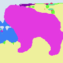
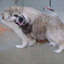
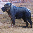
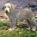
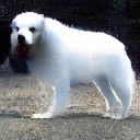
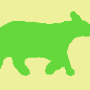
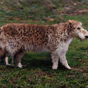
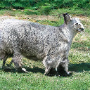
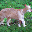
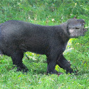
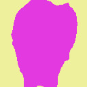
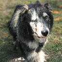
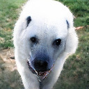
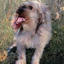
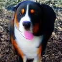
(a) Argmaxed logits of segmentation expert.

$\Phi(x)$	transferred $y=\Lambda(\tau(v|\Phi(x)))$

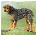
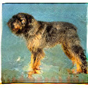
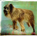
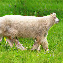
(b) Logits of segmentation expert.

input $x$ transferred $y=\Lambda(\tau(v|\Phi(x)))$

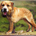
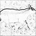
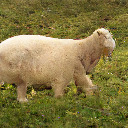
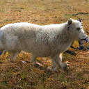
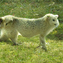
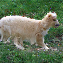
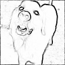
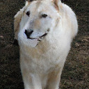
(c) Edge-to-Image using stylized ResNet classifier.

input $x$	transferred $y=\Lambda(\tau(v|\Phi(x)))$

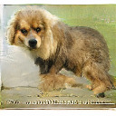
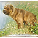
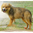
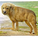
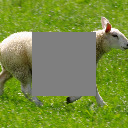
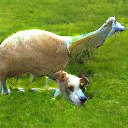
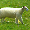
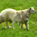
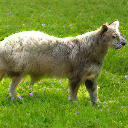
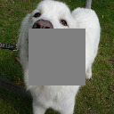
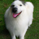
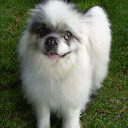
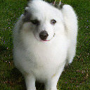
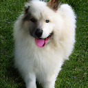
(d) Inpainting using vanilla ResNet classifier.

Figure 3: Different Image-to-Image translation tasks solved with a single AE $g$ and different experts $f$.

The autoencoder is trained on a combination of all carnivorous animal classes in ImageNet and images of the AwA2 dataset [75], split into 211306 training images and 10000 testing images, which we call the Animals dataset. The details regarding architecture and training of this autoencoder are provided in Sec. F.

Image-to-Image Translation:

In Fig. 3, we investigate the translation from different source domain models $\Phi$ onto the same generator $\Lambda$ using our cINN $\tau$. In Fig. 2(a), $f$ is a segmentation network trained on COCOStuff, and $\Phi=f$, i.e. $z_{\Phi}$ is given by the final segmentation output of the network. This case corresponds to a translation from segmentation masks to images and we observe that our approach can successfully fuse the segmentation model with the autoencoder to obtain a wide variety of generated image samples corresponding to a given segmentation mask. Fig. 2(b) uses the same segmentation network for $f$, but this time, $\Phi$ are the logit predictions of the network (visualized by a projection to RGB values). The diversity of generated samples is greatly reduced compared to Fig. 2(a), which indicates that logits still contain a lot of information which are not strictly required for segmentation, e.g. the color of animals. This shows how different layers of an expert can be selected to obtain more control over the synthesis process.

In Fig. 2(c), we consider the task of translating edge images to natural images. Here, $x$ is obtained through the Sobel filter, and we choose a ResNet pretrained for image classification on stylized ImageNet as a domain expert for edge images, as it has shown sensitivity to shapes [25]. This combination of $\Phi$ and $\Lambda$ through $\tau$ enables edge-to-image translation. Fig. 2(d) shows an image inpainting task, where $x$ is a masked image. In this case, large portions of the shape are missing from the image but the unmasked regions contain texture patches. This makes a ResNet pretrained for image classification on ImageNet a suitable domain expert due to its texture bias. The samples demonstrate that textures are indeed faithfully preserved.

Furthermore, we can employ the same approach for generative superresolution. Fig. 4 shows the resulting transfer when using our method for combining two autoencoders, which are trained on different scales. More precisely, $f$ is an autoencoder trained on images of size $32\times 32$, while $g$ is an autoencoder of $256\times 256$ images. The samples show that the model captures the ambiguities w.r.t. this translation and thereby enables efficient superresolution.

$16\times 16$	to $256\times 256$ Animalfaces	$32\times 32$	to $256\times 256$ CelebA-HQ/FFHQ

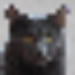
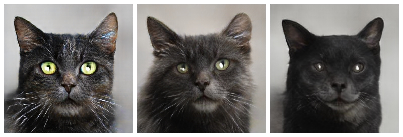
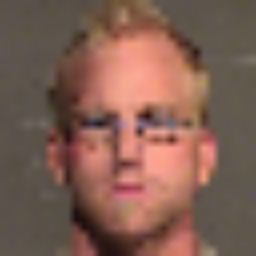
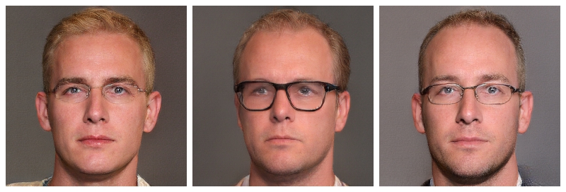
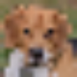
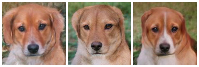
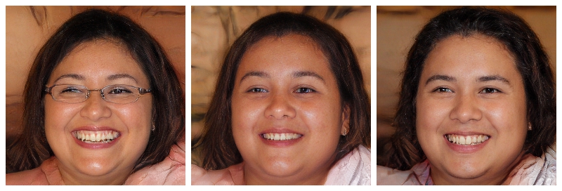
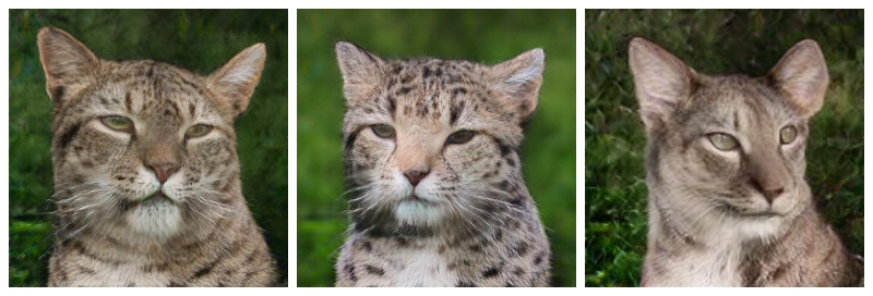
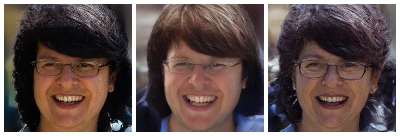
Figure 4: Superresolution with Network-to-Network Translation. Here, we use our cINN to combine two autoencoders $f$ and $g$ to generatively combine two autoencoders living on image scales $32\times 32$ and $256\times 256$.

Model Diagnosis:

$x$	early layer: $\Lambda(z_{\Theta})$	middle layer: $\Lambda(z_{\Theta})$	last layer of $f$: $\Lambda(z_{\Theta})$

Figure 5: Translating different layers of an expert model $f$ to the representation of an autoencoder $g$ reveals the learned invariances of $f$ and thus provides diagnostic insights. Here, $f$ is a segmentation model, while $g$ is the same AE as in Sec. 4.2. For $z_{\Phi}=\Phi(x)$, obtained from different layers of $f$, we sample $z_{\Theta}$ as in Eq. (7) and synthesize corresponding images $\Lambda(z_{\Theta})$.

Besides being applicable for content creation, our approach to recovering the invariances of $f$ can also serve as a diagnostic tool for model interpretation. By comparing the generated samples $y=\Lambda(z_{\Theta})$ (see Eq. (7)) conditioned on representations $z_{\Phi}=\Phi(x)$ extracted from different layers of $f$, we see how the invariances increase with increasing layer depth and can thereby visualize what the model has learned to ignore. Using the same segmentation model $f$ and autoencoder $g$ as described above, we visualize the invariances and model representations for different layers on the Animals and a web-scraped Landscapes dataset. For the latter, Fig. 5 demonstrates how the model $f$ has learned to discard information in later layers; e.g. the variance in the synthesized outputs increases (such as different lightings or colors for the same scene). The corresponding experiment on the Animals dataset is presented in Sec. E. There, we also study the importance of faithfully modeling ambiguities of the translation by replacing the cINN with an MLP, which in contrast to the cINN fails to translate deep representations.

Note that all results in Fig. 3 and Fig. 5, 3(a) were obtained by combining a single, generic autoencoder $g$, which has no capabilities to process inputs of $\mathcal{D}_{x}$ on its own, and different domain experts $f$, which possess no generative capabilities at all. These results demonstrate the feasibility of solving a wide-range of image-to-image tasks through the fusion of pre-existing, task-agnostic experts on image domains $\mathcal{D}_{x},\mathcal{D}_{y}$. Moreover, choosing different layers of the expert $f$ provides additional, fine-grained control over the generation process.

4.3 Evaluating image modification capabilities of our generic approach

input	method	hair	glasses	gender		input	method	beard	age	smiling
	our						our
	[8]						[8]
	our						our
	[8]						[8]
FID	our	15.18	37.32	16.38		FID	our	12.02	10.77	9.57
	[8]	20.94	41.27	20.04			[8]	19.88	21.77	14.47

Figure 6: We directly consider attribute vectors for $z_{\Phi}$ to perform attribute modifications. We show both qualitative comparisons to [8], obtained by changing a single attribute of the input, as well as quantiative comparisons of FID scores, obtained after flipping a single attribute for all images of the test set. The results demonstrate the value of reusing a powerful, generic autoencoder (AE) $g$ and repurposing it via our approach for a specific task, such as attribute modification, instead of learning an AE and the modification task simultaneously.

Attribute Modification:

To compare our generic approach against task-specific approaches, we compare its ability for attribute modification on face images to those of [8]. We train the same autoencoder $g$ as in the previous section on CelebA [42], and directly use attribute vectors as $z_{\Phi}$. For an input image $y$ with attributes $z_{\Phi}$, we synthesize versions with modified attributes $z_{\Phi}^{*}$. In each column of Fig. 6, we flip the binary entry of the corresponding attribute to obtain $z_{\Phi}^{*}$. To obtain the modified image, we first compute $z_{\Theta}=\Theta(y)$ and use its corresponding attribute vector $z_{\Phi}$ to obtain its attribute invariant representation $v=\tau^{-1}(z_{\Theta}|z_{\Phi})$. We then mix it again with the modified attribute vector to obtain $z_{\Theta}^{*}=\tau(v|z_{\Phi}^{*})$, which can be readily decoded to the modified image $y^{*}=\Lambda(z_{\Theta}^{*})$.

Qualitative results in Fig. 6 demonstrate successful modification of attributes. In comparison to [8], our approach produces more coherent changes, e.g. changing gender causes changes in hair length and changes in the beard attribute have no effect on female faces. This demonstrates the advantage of fusing attribute information on a low-dimensional representation of a generic autoencoder. Overall, our approach produces images of higher quality, as demonstrated by the FID scores [31] in Fig. 6. Note that FID-scores are calculated w.r.t. the complete dataset, explaining the high FID scores for attribute glasses, where images consistently possess a large black area.

Exemplar-Guided Translation:

$\Phi(x)$    exemplar $y$

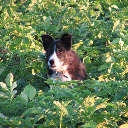
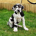
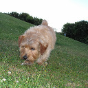
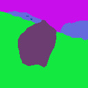
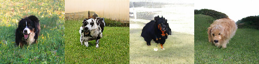
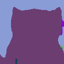
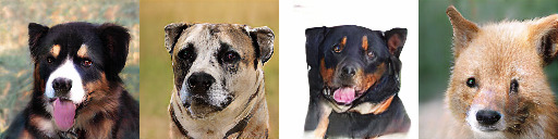
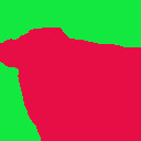
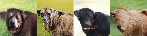
(a) Exemplar-guided image-to-image translation.

$\Phi(x)$    exemplar $y$

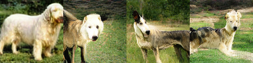
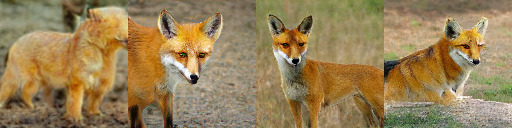
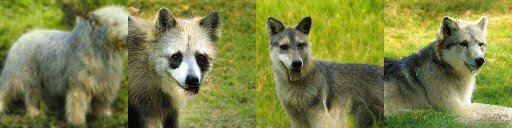
(b) Unsupervised shape and appearance disentangling.

Figure 7: In (a), a segmentation representation $\Phi(x)$ is translated under the guidance of the residual $v=\tau^{-1}(\Theta(y)|\Phi(y))$ obtained from exemplar $y$. In (b), $\Phi$ is the same as $\Theta$, but applied after a spatial deformation of its input such that $\tau$ learns to extract a shape representation into $v$, which then controls the target shape.

Another common image modification task is exemplar-guided image-to-image translation [51], where the semantic content and spatial location is determined via a label map and the style via an exemplar image. To approach this task, we utilize the same segmentation model and autoencoder as in Sec. 4.2. As before, we use the last layer of the segmentation model to represent semantic content and location. For a given exemplar $y$, we can then extract its residual $v=\tau^{-1}(\Theta(y)|\Phi(y))$ and the segmentation representation $z_{\Phi}=\Phi(x)$ of another image $x$. Due to the independence of $v$ and $z_{\Phi}$, we can now transfer $z_{\Phi}$ under the guidance of $v$ to a recombined $z_{\Theta}^{*}=\tau(v|z_{\Phi})$ which is readily decoded to an image $y^{*}=\Lambda(z_{\Theta}^{*})$ as shown in Fig. 3(a).

Unsupervised Disentangling of Shape and Appearance:

Our approach also allows for an unsupervised variant of the previous task, as shown in Fig. 3(b). Here, we use a random spatial deformation $d$ (see Sec. C) to define $\Phi=\Theta\circ d$. Thus, $z_{\Phi}$ and $z_{\Theta}$ share the same appearance but differ in pose, which is distilled into $v$. For exemplar guided synthesis, the roles of $x$ and $y$ are now swapped.

Unpaired Image Translation:

Fig. 8 demonstrates results of our approach applied to unpaired image-to-image translation. Here, we use the same setup as for attribute modification, but train various cINN models for unpaired transfer between the following datasets: CelebA and AnimalFaces-HQ [9], FFHQ and CelebA-HQ [34], Anime [3] to CelebA-HQ/FFHQ and Oil Portraits to CelebA-HQ/FFHQ. Details regarding the training procedure can be found in the Sec. D.

5 Conclusion

This paper has addressed the problem of generic domain transfer between arbitrary fixed off-the-shelf domain models. We have proposed a conditionally invertible domain translation network that faithfully transfers between existing domain representations without altering them. Consequently, there is no need for costly or potentially even infeasible retraining or finetuning of existing domain representations. The approach is (i) flexible: Our cINN for translation as well as its optimization procedure are independent from the individual domains and, thus, provide plug-and-play capabilities by allowing to plug in arbitrary existing domain representations; (ii) powerful: Enabling the use of pretrained expert domain representations outsources the domain specific learning task to these models. Our model can thus focus on the translation alone which leads to improvements over previous approaches; (iii) convenient and affordable: Users can now utilize powerful, pretrained models such as BERT and BigGAN for new tasks they were not designed for, with just a single GPU instead of the vast multi-GPU resources required for training such domain models. Future applications include transfer between diverse domains such as speech, music or brain signals.

Oil-Portrait to Photography	Anime to Photography	FFHQ to CelebA-HQ	FFHQ to AFHQ

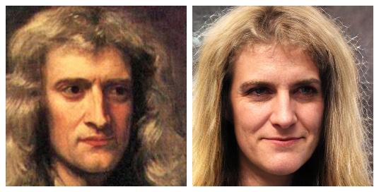
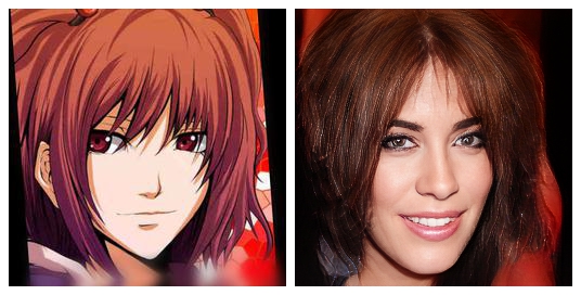
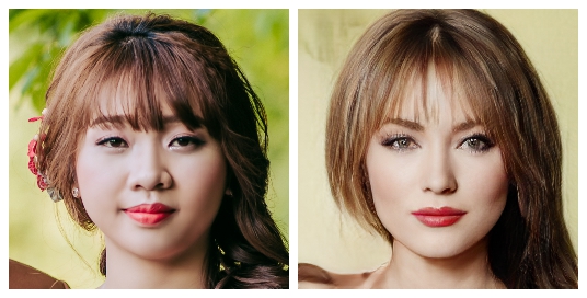
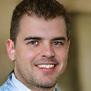
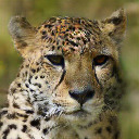
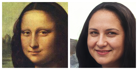
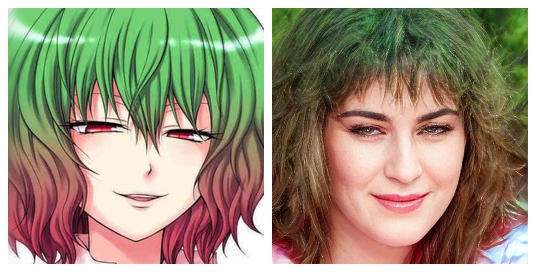
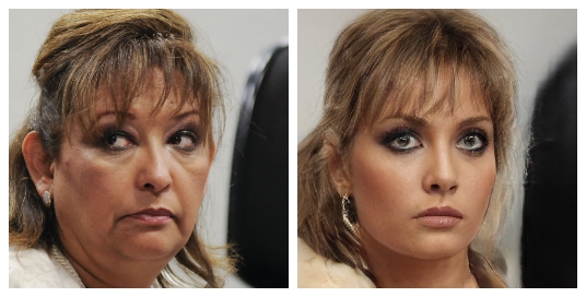
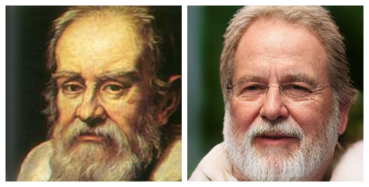
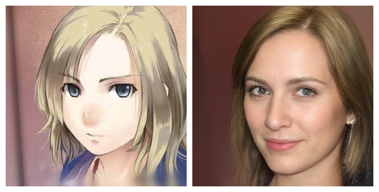
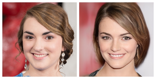
Figure 8: Unpaired Transfer: Bringing oil portraits and animes to live by projecting them onto the FFHQ dataset (column 1 and 2, respectively). Column 3 visualizes the more subtle differences introduced when translating between different datasets of human faces such as FFHQ and CelebA-HQ. Column 4 shows a translation between the more diverse modalities of human and animal faces. See also Sec. 4.3 and D.

Broader Impact

Environmental and Economic Aspects:

Single training runs of large scale models have a large environmental footprint due to the massive computational requirements. It is therefore unreasonable to repeat this effort for every new application. Instead we allow to reuse powerful models, leading to significant reductions in computational demands.

Boosting serendipity:

New (scientific) knowledge arises where seemingly unrelated entities are brought together to study their relationship (cf. the ’double projection’ proposed by Heinrich Wölfflin a century ago for art history and other image disciplines to easily contextualize diverse imagery of different cultures). Allowing to efficiently connect expert models for diverse data and problems, thus promises to provide the basis for new directions of future research.

Interdisciplinary research:

One of the main stumbling blocks for interdisciplinary research (e.g. vision and language) is to bring together expert models for widely different domains. State-of-the-art models are typically developed in and for the individual disciplines. Being able to efficiently combine these disciplinary expert models to solve interdisciplinary problems promises to be an enabling factor for more effective cross-disciplinary research.

Social equality:

Training state-of-the art models is typically so costly that only wealthy institutions can afford their transfer and application to different input domains or other subsequent research that would require to retrain them. Computationally efficient transfer of existing models with no need for costly retraining therefore increases the opportunities for economically weaker institutions and countries to have research programs in this field.

Increasing applicability and impact of research output:

Large scale research is often funded by public resources and thus there is a responsibility to make results accessible to the public. While pretrained models are often shared publicly, the scope in which they can be applied is significantly widened by our approach.

Content creation and manipulation:

Domain transfer applied to controlled image synthesis and modification has wide applicability in the creative industry and beyond. However, it can also be misused for forgery and manipulation.

Overview

This appendix provides supplementary material for our work Network-to-Network Translation with cINNs. Firstly, in Sec. A, we discuss and compare computational requirements and resulting costs of our model to other approaches, e.g. BigGAN. Next, in Sec. B, we provide a derivation of the training objective (see Eq.(4)). Its interpretation as an information bottleneck allows for unsupervised disentangling of shape and appearance, which is demonstrated in Sec. C and Fig. S1. Sec. D then provides additional examples (Fig. S2) and technical details for the unpaired image translation as presented in Fig. 8 (Sec. 4.3). Subsequently, we continue with an ablation study in Sec. E, where we analyze the performance of our approach by replacing the conditional invertible neural network with a multilayer perceptron. Next, Sec. F presents the architecture and training procedure of our reusable autoencoder model $g$, which we used to obtain the results shown in Fig. 3, 5, 3(a), 3(b), S1, S4, S5 and S6. Finally, Sec. G provides details on (i) the architecture of the cINN and (ii) the translation from BERT to BigGAN, c.f. Sec. 4.1.

Appendix A Computational Cost and Energy Consumption

In Tab. 11 we compare computational costs of our cINN to those of BERT, BigGAN and FUNIT. The Table shows that, once strong domain experts are available, they can be repurposed by our approach in a time-, energy- and cost-effective way. With training costs of our cINN being two orders of magnitude smaller than the training costs of the domain experts, the latter are amortized over all the new tasks that can be solved by recombining experts with our approach.

Model	Time [days]	Hardware	Energy [kWh]	Cost [EUR]	$CO_{2}$ [kg]
our cINN	$\mathbf{\leq 1}$	1 NVIDIA Titan X	14.4	3.11	4.26
BigGAN [4]	15	8 NVIDIA V100	1260.0	272.16	372.96
FUNIT [41]	14	8 NVIDIA V100	1176.0	254.02	348.10
BERT [15]	10.3	8 NVIDIA V100	865.2	186.88	256.10

Table S0: Comparison of computational costs for a single training run of different models. Energy consumption of a Titan X is based on the recommended system power (0.6 kW) by NVIDIA, and energy consumption of eight V100 on the power (3.5 kW) of a NVIDIA DGX-1 system. Costs are based on the average price of 0.216 EUR per kWh in the EU, and CO2 emissions on the average emissions of 0.296 kg CO2 per kWh in the EU.

Appendix B Training Objective

Derivation of Eq. (4):

For a given $z_{\Phi}$, we use a change of variables, $v=\tau^{-1}(z_{\Theta}|z_{\Phi})$, to express the KL divergence with an integral over $z_{\Theta}$:

$$\operatorname{KL}(p(v|z_{\Phi})|q(v)) =\int_{v}p(v|z_{\Phi})\log\frac{p(v|z_{\Phi})}{q(v)}$$ (8)

$$=\int_{z_{\Theta}}p(\tau^{-1}(z_{\Theta}|z_{\Phi})|z_{\Phi})|\det J_{\tau^{-1}}(z_{\Theta}|z_{\Phi})|\log\frac{p(\tau^{-1}(z_{\Theta}|z_{\Phi})|z_{\Phi})}{q(\tau^{-1}(z_{\Theta}|z_{\Phi}))}$$ (9)

By definition of $v$ in Eq. (3), the invertibility of $\tau$ allows us to express the conditional probability density function $p(v|z_{\Phi})$ of $v$ in terms of the conditional probability density function $p(z_{\Theta}|z_{\Phi})$ of $z_{\Theta}$:

$$p(v|z_{\Phi})=p(\tau(v|z_{\Phi})|z_{\Phi})|\det J_{\tau}(v|z_{\Phi})|$$ (10)

For $v=\tau^{-1}(z_{\Theta}|z_{\Phi})$, the inverse function theorem then implies

$$p(\tau^{-1}(z_{\Theta}|z_{\Phi})|z_{\Phi})=p(z_{\Theta}|z_{\Phi})|\det J_{\tau^{-1}}(z_{\Theta}|z_{\Phi})|^{-1}$$ (11)

Using Eq. (11) in Eq. (9) gives

$$\operatorname{KL}(p(v|z_{\Phi})|q(v)) =\int_{z_{\Theta}}p(z_{\Theta}|z_{\Phi})\log\frac{p(z_{\Theta}|z_{\Phi})}{q(\tau^{-1}(z_{\Theta}|z_{\Phi}))|\det J_{\tau^{-1}}(z_{\Theta}|z_{\Phi})|}$$ (12)

$$=\mathbb{E}_{z_{\Theta}}\left\{-\log q(\tau^{-1}(z_{\Theta}|z_{\Phi}))-\log|\det J_{\tau^{-1}}(z_{\Theta}|z_{\Phi})|+\log p(z_{\Theta}|z_{\Phi})\right\}$$ (13)

Taking the expectation over $z_{\Phi}$ results in Eq. (4).

Appendix C Unsupervised Disentangling of Shape and Appearance

$x$      $y$

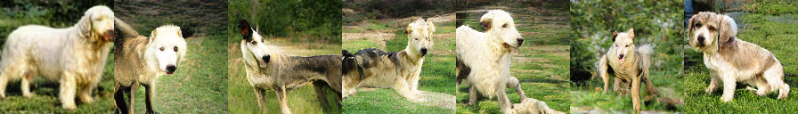
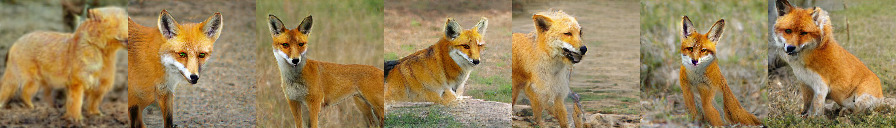
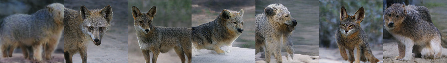
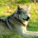
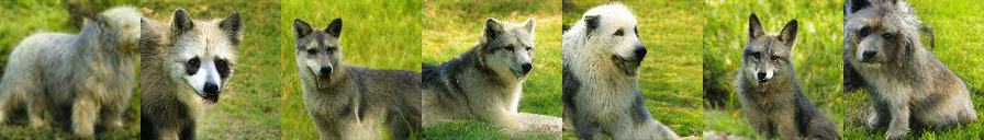
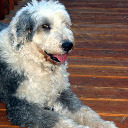
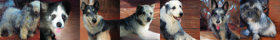
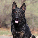
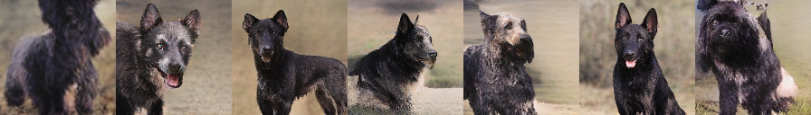
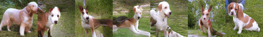
Figure S1: Unsupervised disentangling of shape and appearance. Training our approach on synthetically deformed images, $\tau$ learns to extract a disentangled shape representation $v$ from $y$, which can be recombined with arbitrary appearances obtained from $x$. See also Sec. C.

Unsupervised disentangling of shape and appearance aims to recombine shape, i.e. the underlying spatial structure, from one image with the appearance, i.e. the style, of another image. In contrast to Unpaired Image-to-Image translation of Sec. D, training data does not come partitioned into a discrete set of different image domains, and in contrast to Exemplar-Guided Translation of Sec. 4.3, the task assumes that no shape expert, e.g. a segmentation model, is available. To handle this setting, we use the encoder $\Theta$ of the autoencoder trained on Animals also for $\Phi$, but always apply a spatial deformation to its inputs. Thus, the pairs $(x,y)$ are given by $(d(y),y)$, where $y$ are the original images from the Animals dataset and $d$ is a random combination of horizontal flipping, a thin-plate-spline transformation and cropping. The translation task then consists of the translation of deformed encodings $z_{\Phi}=\Phi(d(y))\coloneqq\Theta(d(y))$ to the original encoding $z_{\Theta}=\Theta(y)$. After training, we apply our translation network to original images without the transformation $d$. For two images $x$ and $y$, we obtain a shape representation of $y$ from its residual $v=\tau^{-1}(\Theta(y)|\Theta(y))$ and recombine it with the appearance of $x$ to obtain $y^{*}=\Lambda(\tau(v|\Theta(x)))$.

in
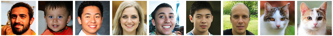
out
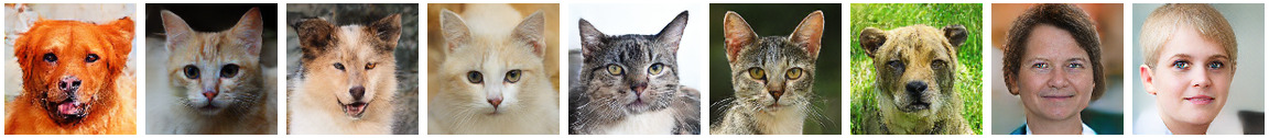
in
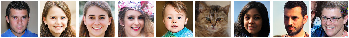
out

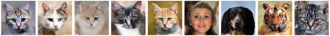
Figure S2: Additional examples for unpaired translation between human and animal faces as in Fig. 8. Our approach naturally provides translations in both directions (see Sec. D). Inputs are randomly choosen test examples from either the human or the animal data and translated to the respective other one.

photography
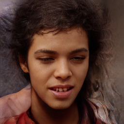
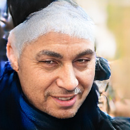
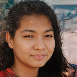
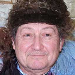
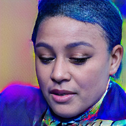
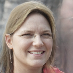
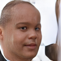
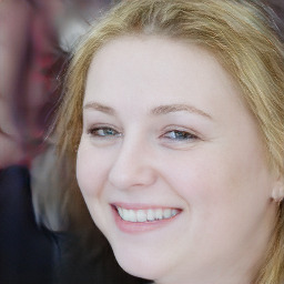
oil portrait
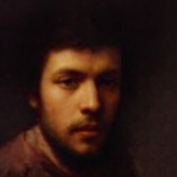
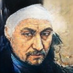
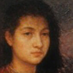
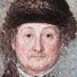
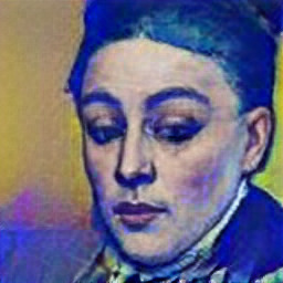
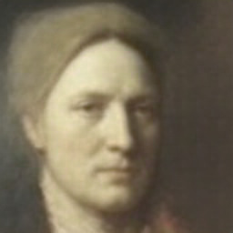
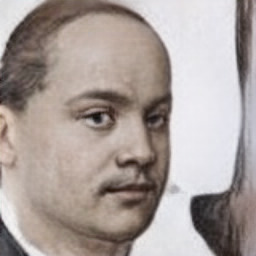
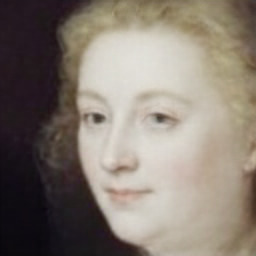
photography
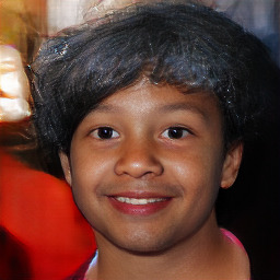
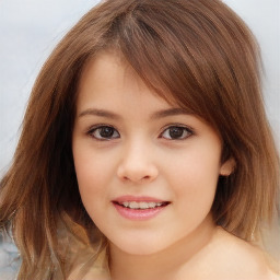
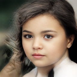
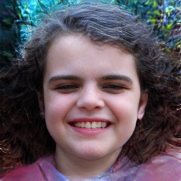
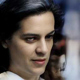
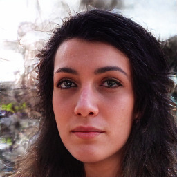
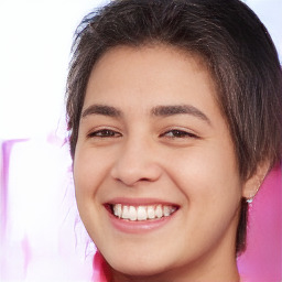
anime

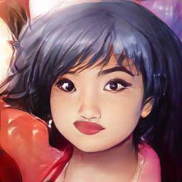
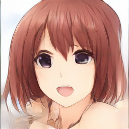
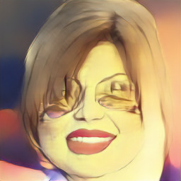
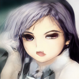
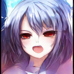
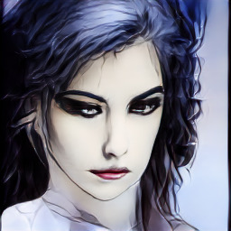
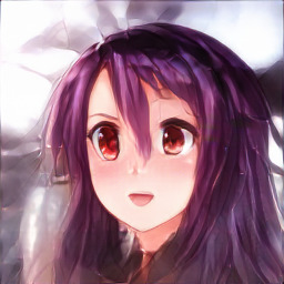
Figure S3: Additional examples for unpaired translation of Oil Portraits to FFHQ/CelebA-HQ and Anime to FFHQ/CelebA-HQ. Here, we show samples where the same $v$ is projected onto the respective dataset.

The results in Fig. S1 demonstrate that our translation network succesfully learns a shape representation $v$, which is independent of the appearance and can thus be recombined with arbitrary appearances, see Eq. (6). Being able to operate completely unsupervised demonstrates the generality of our approach.

Appendix D Unpaired Image Translation

Unpaired Image-to-Image translation considers the case where only unpaired training data is available. Following [87], let $Y^{0}=\{y^{0}_{i}\}_{i=1}^{N}$ be a source set, and $Y^{1}=\{y^{1}_{j}\}_{j=1}^{M}$ a target set. The goal is then to learn a translation from source set to target set, with no information provided as to which $y^{0}_{i}$ matches which $y^{1}_{j}$. We formulate this task as a translation from a set indicator $x\coloneqq z_{\Phi}\in\{0,1\}$ to an output $y$, such that for $z_{\Phi}=0$, $y$ belongs to the source set $Y^{0}$, and for $z_{\Phi}=1$, $y$ belongs to the target set. Thus, in the case of unpaired image translation, the domains are given by $\mathcal{D}_{x}=\{0,1\}$ and $\mathcal{D}_{y}=Y^{0}\cup Y^{1}$, with training pairs $\{(0,y^{0}_{i})|i=0,\dots,N\}\cup\{(1,y^{1}_{j})|j=0,\dots,M\}$. Because the residual $v$ is independent of $z_{\Phi}$, it captures precisely the commonalities between source and target set and therefore establishes meaningful correspondences between them. To translate $y^{0}_{i}$, we first obtain its residual $v=\tau^{-1}(\Theta(y^{0}_{i})|0)$, and then decode it as an element of the target set $y^{*}=\Lambda(\tau(v|1))$. Note that the autoencoder $g=\Lambda\circ\Theta$ is always trained on the combined domain $\mathcal{D}_{y}=Y^{0}\cup Y^{1}$, i.e. a combination of the two datasets of interest.

Additional examples for unpaired translation as in Fig. 8 can be found in Fig. S2. One can see that the viewpoint of a face is preserved upon translation, which demonstrates that $v$ learns semantic correspondences between the pose of faces from different dataset modalities, without any paired data between them. The same holds for the samples in Fig. S3, where the same $v$ is projected onto different domains $\mathcal{D}_{x}$.

Appendix E Ablation Study: Replacing our cINN with an MLP

$x$	method	early layer: $\Lambda(z_{\Theta})$	middle layer: $\Lambda(z_{\Theta})$	last layer of $f$: $\Lambda(z_{\Theta})$
	our
	MLP
	our
	MLP
	our
	MLP
	our
	MLP
	our
	MLP
FID	our	$34.0\pm 0.1$	$23.4\pm 0.7$	$27.6\pm 0.1$
	MLP	$24.2$	$25.6$	$264.0$

Figure S4: Model diagnosis compared to a MLP for the translation. Synthesized samples and FID scores demonstrate that a direct translation with a multilayer perceptron (MLP) does not capture the ambiguities of the translation process and can thus only produce a mean image. In contrast, our cINN correctly captures the variability and produces coherent outputs.

To illustrate the importance of the cINN to model ambiguities of the translation, we demonstrate the effect of replacing our cINN with a (deterministic) multilayer perceptron (MLP) in Fig. S4. The MLP consists of two parts: (i) an embedding part as in Tab. 2(b) and (ii) the architecture of a fully-connected network which was recently used for neural scene rendering [46]. We perform the same model diagnosis experiment as in Fig. 5, but applied to the Animals dataset. For early layers, the translation contains almost no ambiguity and can be handled successfully by both the cINN and the MLP. For a deeper layer of the used segmentation model $f$, the translation has moderate ambiguities, as $f$’s invariances w.r.t. to the input increase. This is not accurately reflected by the multilayer perceptron, because it does not model the space of these invariances. Finally, for the last layer of $f$, the MLP predicts the mean over all possible translation outputs which, due to its large ambiguities, does not result in a meaningful translation anymore, whereas our cINN still samples coherent translation outputs. FID scores in Tab. S4 further validate this behavior for the whole test set.

Appendix F Architecture and Training of the Autoencoder $g$

$\Phi(x)$    exemplar $y$

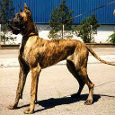
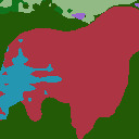
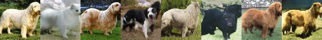
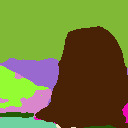
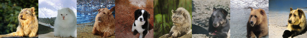
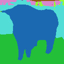
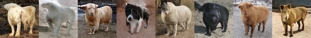
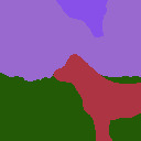
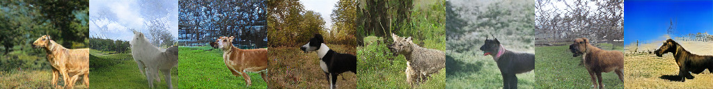
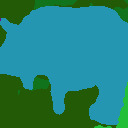
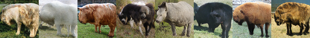
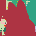
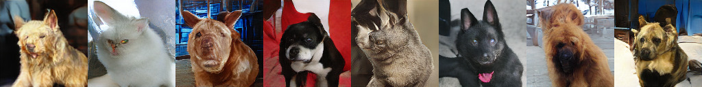
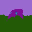
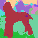
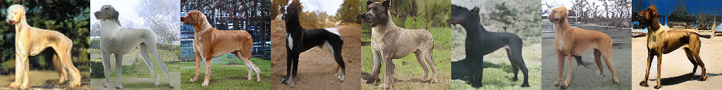
Figure S5: Additional examples for exemplar-guided image-to-image translation as in Fig. 3(a).

$\Phi(x)$	translating $\Phi(x)$ onto target domain of AE $g$ with different samples $v\sim q(v)$

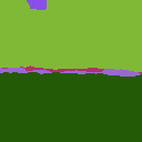
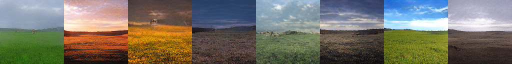
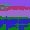
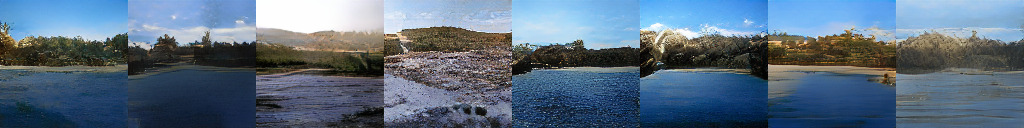
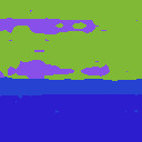
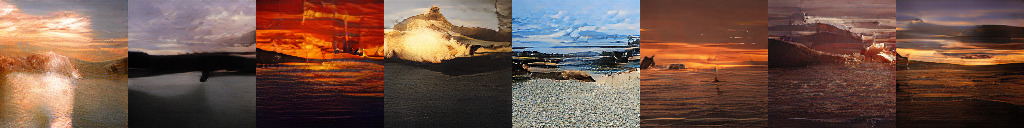
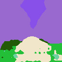
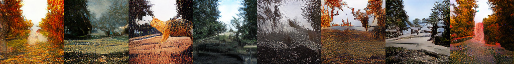
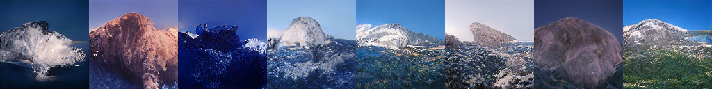
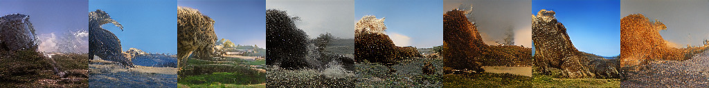
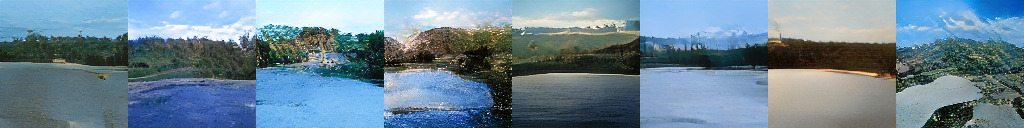
Figure S6: Additional Landscape samples, obtained by translation of the argmaxed logits (i.e. the segmentation output) of the segmentation model from Sec. 4.2, 4.3 into the space of our autoencoder $g$, see Sec. 4.2, 4.3. The synthesized examples demonstrate that our approach is able to generate diverse and realistic images from a given label map or through a segmentation model.

All experiments in Sec. 4.2, the exemplar-guided image-to-image translation in Sec. 4.3 as well as the additional results in Fig. S5 and Fig. S6 were conducted using the same (i.e. same weights and architecture) autoencoder $g$, thereby demonstrating how a single model can be re-used for multiple purposes within our framework.
For the autoencoder, we use a ResNet-101 [29] architecture as encoder $\Theta$, and the BigGAN architecture as the decoder $\Lambda$, see Tab. S1. As we do not use class information, we feed the latent code $z_{\Theta}$ of the encoder into a a fully-connected layer and use its softmax-activated output as a replacement for the one-hot class vector used in BigGAN. The encoder predicts mean $\Theta(y)_{\mu}$ and diagonal covariance $\Theta(y)_{\sigma^{2}}$ of a Gaussian distribution and we use the reparameterization trick to obtain samples $z_{\Theta}=\Theta(y)_{\mu}+\operatorname{diag}(\Theta(y)_{\sigma^{2}})\epsilon$ of the latent code, where $\epsilon\sim\mathcal{N}(0,\mathbb{1})$. For the reconstruction loss $\|\cdot\|$, we use a perceptual loss based on features of a pretrained VGG-16 network [64], and, following [13], include a learnable, scalar output variance $\gamma$. Additionally, we use the PatchGAN discriminator $\mathcal{D}$ from [33] for improved image quality. Hence, given the autoencoder loss

$$\mathcal{L}_{VAE}(\Theta,\Lambda,\gamma)=\mathbb{E}_{\begin{subarray}{l}y\sim p(y)\\ \epsilon\sim\mathcal{N}(0,\mathbb{1})\end{subarray}} \bigg{[}\frac{1}{\gamma}\|y-\Lambda(\Theta_{\mu}(y)+\sqrt{\operatorname{diag}(\Theta_{\sigma^{2}}(y))}\;\epsilon)\|+\log\gamma$$

$$+\operatorname{KL}\big{(}\mathcal{N}\left(z_{\Theta}|\Theta_{\mu}(y),\operatorname{diag}(\Theta_{\sigma^{2}}(y)\big{)}\|\mathcal{N}(0,\mathbb{1})\right)\bigg{]},$$ (14)

and the GAN-loss

$$\mathcal{L}_{GAN}(g,\mathcal{D})=\mathbb{E}_{\begin{subarray}{l}y\sim p(y)\\ \epsilon\sim\mathcal{N}(0,\mathbb{1})\end{subarray}}\left[\log\mathcal{D}(y)+\log\left(1-\Lambda\Big{(}\Theta_{\mu}(y)+\sqrt{\operatorname{diag}(\Theta_{\sigma^{2}}(y))}\;\epsilon\Big{)}\right)\right],$$ (15)

the total objective for the training of $g=\{\Theta,\Lambda,\gamma\}$ reads:

$$\{\Theta^{*},\Lambda^{*},\gamma^{*}\}=\arg\min_{\Theta,\Lambda,\gamma}\max_{\mathcal{D}}\left[\mathcal{L}_{VAE}(\Theta,\Lambda,\gamma)+\lambda\mathcal{L}_{GAN}(\{\Theta,\Lambda,\gamma\},\mathcal{D})\right].$$ (16)

This is similar to the improved image metric suggested in [20], but in contrast to their work, we use an adaptive weight $\lambda$, computed by the ratio of the gradients of the decoder $\Lambda$ w.r.t. its last layer $\Lambda_{L}$:

$$\lambda=\frac{\|\nabla_{\Lambda_{L}}(\mathcal{L}_{rec})\|}{\|\nabla_{\Lambda_{L}}(\mathcal{L}_{GAN})\|+\delta}$$ (17)

where the reconstruction loss $\mathcal{L}_{rec}$ is given as (c.f. Eq. (14)):

$$\mathcal{L}_{rec}=\mathbb{E}_{\begin{subarray}{l}y\sim p(y)\\ \epsilon\sim\mathcal{N}(0,\mathbb{1})\end{subarray}}\bigg{[}\frac{1}{\gamma}\|y-\Lambda(\Theta_{\mu}(y)+\sqrt{\operatorname{diag}(\Theta_{\sigma^{2}}(y))}\;\epsilon)\|+\log\gamma\bigg{]},$$ (18)

and a small $\delta$ is added for numerical stability.

RGB image $x\in\mathbb{R}^{128\times 128\times 3}$

Conv down $\to\mathbb{R}^{64\times 64\times 64}$

Norm, ReLU, MaxPool $\to\mathbb{R}^{32\times 32\times 64}$

$3\times$ BottleNeck $\to\mathbb{R}^{32\times 32\times 256}$

$4\times$ BottleNeck down $\to\mathbb{R}^{16\times 16\times 512}$

$23\times$ BottleNeck down $\to\mathbb{R}^{8\times 8\times 1024}$

$3\times$ BottleNeck down $\to\mathbb{R}^{4\times 4\times 2048}$

AvgPool, FC $\mapsto(\mu,\sigma^{2})\in\mathbb{R}^{128}\times\mathbb{R}^{128}$

(a) Encoder based on Resnet-101.

$\bar{z}\in\mathbb{R}^{128}\sim\mathcal{N}(\mu,\operatorname{diag}(\sigma^{2}))$

$3\times$ (FC, LReLU) $\to\mathbb{R}^{256}$

FC, Softmax $\to\mathbb{R}^{1000}$

Embed $\mapsto h\in\mathbb{R}^{128}$

FC($\bar{z}$) $\to\mathbb{R}^{4\times 4\times 16\cdot 96}$

ResBlock($\bar{z}$,$h$) up $\to\mathbb{R}^{8\times 8\times 16\cdot 96}$

ResBlock($\bar{z}$,$h$) up $\to\mathbb{R}^{16\times 16\times 8\cdot 96}$

ResBlock($\bar{z}$,$h$) up $\to\mathbb{R}^{32\times 32\times 4\cdot 96}$

ResBlock($\bar{z}$,$h$) up $\to\mathbb{R}^{64\times 64\times 2\cdot 96}$

Non-Local Block $\to\mathbb{R}^{64\times 64\times 2\cdot 96}$

ResBlock($\bar{z}$,$h$) up $\to\mathbb{R}^{64\times 64\times 96}$

Norm, ReLU, Conv up $\to\mathbb{R}^{128\times 128\times 3}$

Tanh $\mapsto\bar{x}\in\mathbb{R}^{128\times 128\times 3}$

(b) Decoder based on BigGAN.

Table S1: Autoencoder architecture for the CelebA and Animals datasets at resolution $128\times 128$.

Appendix G Implementation Details

G.1 Architecture of the conditional INN

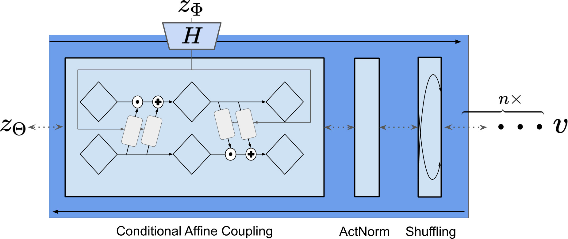
Figure S7: A single (conditionally) invertible block used to build our cINN. We build the cINN from $n=20$ of these blocks for all of our experiments.

input $z\in\mathbb{R}^{d}$

(FC, LReLU) $\rightarrow\mathbb{R}^{8\cdot d}$

$2\times$ (FC, LReLU) $\rightarrow\mathbb{R}^{8\cdot d}$

(FC, LReLU) $\rightarrow\mathbb{R}^{d}$

(a) Basic fully connected architecture.

input $y\in\mathbb{R}^{c\times h\times w}$

$n\times$ Conv down, ActNorm, LReLU

$\rightarrow\mathbb{R}^{64\cdot n\times h/2^{n}\times w/2^{n}}$

Flatten, FC $\rightarrow\mathbb{R}^{d}$

(b) Embedding module $H$, see Eq. (19).

Table S2: (a): Architecture of the subnetworks $s_{\theta}$ and $t_{\theta}$ used to build the normalizing flow described in Sec. 3, G.1. Leaky ReLU (LReLU) uses a slope parameter $\alpha=0.01$. For the cINN from Sec. 4.1, $d=268$, while for Sec. 4.2 and Sec. 4.3, $d=128$. (b) Architecture of the embedding module $H$, which is used to pre-process arbitrarily sized conditioning information $y$ via $h=H(y)$. Here, $n$ denotes the number of downsampling steps. If the conditioning $y$ does not have spatial dimensionality, we replace the whole network by a simple feedforward-architecture as in Tab. 2(a).

In our implementation, the conditional invertible neural network (cINN) consists of a sequence of INN-blocks as shown in Fig. S7, and a non-invertible embedding module $H$ which provides the conditioning information. Each INN-block is build from (i) an alternating affine coupling layer [17], (ii) an activation normalization (actnorm) layer [35], and (iii) a fixed permutation layer, which effectively mixes the components of the network’s input. Given an input $z\in\mathbb{R}^{D}$ and additional conditioning information $y$, we pre-process the latter with a neural network $H$ as

$$h=H(y),$$ (19)

and a single conditional affine coupling layer splits $z$ into two parts $z_{1:d}$, $z_{d+1:D}$ and computes

$$z_{1:d},z_{d+1:D} =\text{{split}}(z)$$ (20)

$$z^{\prime} =\text{{concat}}\Big{(}z_{1:d},s_{\theta}([z_{1:d};h])\odot z_{d+1:D}+t_{\theta}([z_{1:d};h])\Big{)}$$ (21)

where $s_{\theta}$ and $t_{\theta}$ are implemented as simple feedforward neural networks, which process the concatenated input $[z_{i:j},h]$ (see Tab. 2(a)). The alternating coupling layer ensures mixing for all components of $z$:

$$z^{\prime\prime} =\text{{concat}}\Big{(}s_{\theta}([z^{\prime}_{d+1:D};h])\odot z_{1:d}+t_{\theta}([z^{\prime}_{d+1:D};h]),z^{\prime}_{d+1:D}\Big{)}.$$ (22)

We implement the embedding module $H$ as a simple (convolutional) neural network, see Tab. 2(b) for details regarding its architecture. Note that $H$ does not need to be invertible as it soley processes conditioning information. Hence, given some $h=H(y)$, the network $\tau$ is conditionally invertible. Usually, we train with a batch size of 10-25, which requires 4-12 GB VRAM and converges in less than a day.

G.2 Training Details for Bert-to-BigGAN Translation

source domain $x$	target domain $y$			source domain $x$	target domain $y$
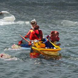
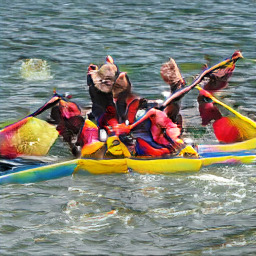
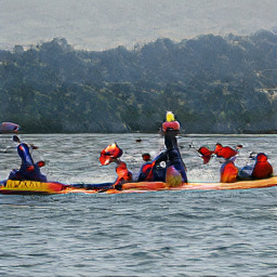
Two people on a paddle boat in the water				A close up of a plant with broccoli
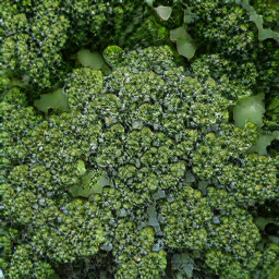
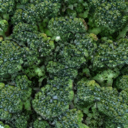
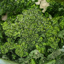
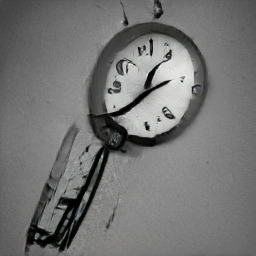
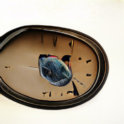
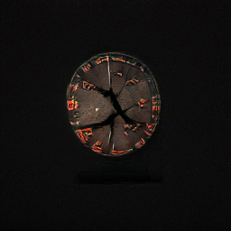
A close up of a clock on a wall				A fighter jet flying through a cloudy sky
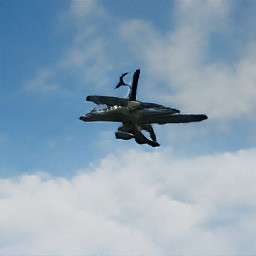
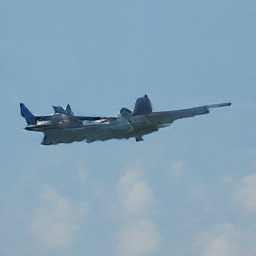
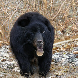
A black bear is walking through the woods				A glass of wine sitting on a table
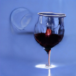
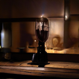
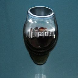
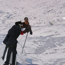
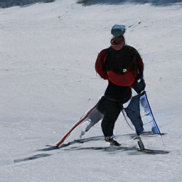
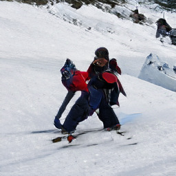
A man riding skis down a snow covered slope				A wooden chair sitting in front of a chair
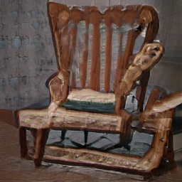
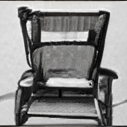
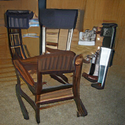
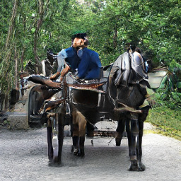
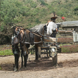
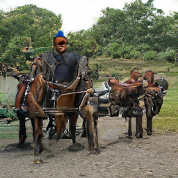
A group of horses pulling a carriage down a dirt				A car parked in front of a building

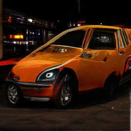
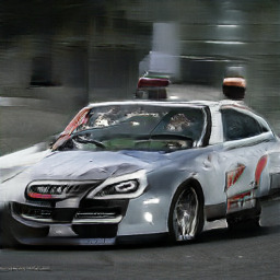
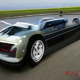
Figure S8: BERT [15] to BigGAN [4] transfer: Additional examples, which demonstrate high diversity in synthesized outputs.

Training our approach to translate between a model’s $f$ representation $z_{\Phi}=\Phi(x)$ and BigGAN’s latent space $z_{\Theta}$ requires to dequantize the discrete class labels $c$ that BigGAN is trained with. To do so, we consider the stacked vector

$$z_{\Theta}^{\prime}=\left[\tilde{z},Wc\right],$$ (23)

consisting of $\tilde{z}\sim\mathcal{N}(0,\mathbb{1})$, $\tilde{z}\in\mathbb{R}^{140}$, sampled from a multivariate normal distribution and $c\in\{0,1\}^{K}$, a one-hot vector specifying an ImageNet class ($K=1000$ classes in total). The matrix $W$, a part of the generator $\Lambda$, maps the one-hot vector $c$ to $h\in\mathbb{R}^{128}$, i.e. $h=Wc$, such that $z_{\Theta}^{\prime}$ in Eq. (23) corresponds to a synthesized image, given a pretrained generator of BigGAN. However, as $c$ contains discrete labels, we have to avoid collapse of $\tau$ onto a single dimension of $h$ during training. To this end, we pass the vector $h$ through a small, fully connected variational autoencoder (described in Tab. S3) and replace $h$ by its stochastic reconstruction $\hat{h}$, which effectively performs dequantization, such that:

$$z_{\Theta}=\left[\tilde{z},\hat{h}\right],\quad\text{with}\;z_{\Theta}\in\mathbb{R}^{268}.$$ (24)

Training of $\tau$ is then conducted by sampling $z_{\Theta}$ as in Eq. (24) and minimizing the objective described in Eq. (4), i.e. finding a mapping $\tau$ that conditionally maps $z_{\Phi}$ and the corresponding ambiguities $v\sim\mathcal{N}(0,\mathbb{1})$ to $g$’s representations $z_{\Theta}$. Additional results obtained when using this approach to conditionally translate BERT’s representation $z_{\Phi}$ into the latent space of BigGAN (see also Sec. 4.1) can be found in Fig. S8.

Embedding $h\in\mathbb{R}^{128}$

$3\times$ (FC, LReLU) $\rightarrow\mathbb{R}^{4096}$

(FC, LReLU) $\rightarrow\mathbb{R}^{128}$

$\mu,\sigma^{2}$: for each:

$3\times$ (FC, LReLU) $\rightarrow\mathbb{R}^{4096}$

(FC, LReLU) $\rightarrow\mathbb{R}^{128}$

$h\in\mathbb{R}^{128}\sim\mathcal{N}(\mu,\operatorname{diag}(\sigma^{2}))$

$4\times$ (FC, LReLU) $\rightarrow\mathbb{R}^{4096}$

(FC, LReLU) $\rightarrow\mathbb{R}^{128}$

Table S3: Training a cINN on synthetic BigGAN data requires to dequantize the discrete class information which is used as conditioning information for the decoder. To this end, we make use of a variational autoencoder as described in Sec. G.2, which provides a stochastic reconstruction of its input $h$. For Leaky ReLU, we use a slope parameter of $\alpha=0.01$.

References

- [1] Alexander A. Alemi, Ian Fischer, Joshua V. Dillon, and Kevin Murphy. Deep Variational Information Bottleneck. In 5th International Conference on Learning Representations, ICLR, 2017.
- [2] Tadas Baltrusaitis, Chaitanya Ahuja, and Louis-Philippe Morency. Multimodal Machine Learning: A Survey and Taxonomy. IEEE Transactions on Pattern Analysis and Machine Intelligence, 2019.
- [3] Gwern Branwen, Anonymous, and Danbooru Community. Danbooru2019 portraits: A large-scale anime head illustration dataset. https://www.gwern.net/Crops#danbooru2019-portraits, March 2019.
- [4] Andrew Brock, Jeff Donahue, and Karen Simonyan. Large Scale GAN Training for High Fidelity Natural Image Synthesis. In 7th International Conference on Learning Representations, ICLR, 2019.
- [5] Tom B. Brown, Benjamin Mann, Nick Ryder, Melanie Subbiah, Jared Kaplan, Prafulla Dhariwal, Arvind Neelakantan, Pranav Shyam, Girish Sastry, Amanda Askell, Sandhini Agarwal, Ariel Herbert-Voss, Gretchen Krueger, Tom Henighan, Rewon Child, Aditya Ramesh, Daniel M. Ziegler, Jeffrey Wu, Clemens Winter, Christopher Hesse, Mark Chen, Eric Sigler, Mateusz Litwin, Scott Gray, Benjamin Chess, Jack Clark, Christopher Berner, Sam McCandlish, Alec Radford, Ilya Sutskever, and Dario Amodei. Language Models are Few-Shot Learners. arXiv preprint arXiv:2005.14165, 2020.
- [6] Liang-Chieh Chen, G. Papandreou, I. Kokkinos, Kevin Murphy, and A. Yuille. DeepLab: Semantic Image Segmentation with Deep Convolutional Nets, Atrous Convolution, and Fully Connected CRFs. IEEE Transactions on Pattern Analysis and Machine Intelligence, 2018.
- [7] Qifeng Chen and Vladlen Koltun. Photographic Image Synthesis with Cascaded Refinement Networks. In IEEE International Conference on Computer Vision, ICCV, 2017.
- [8] Yunjey Choi, Minje Choi, Munyoung Kim, Jung-Woo Ha, Sunghun Kim, and Jaegul Choo. StarGAN: Unified Generative Adversarial Networks for Multi-Domain Image-to-Image Translation. In Proceedings of the IEEE Conference on Computer Vision and Pattern Recognition, 2018.
- [9] Yunjey Choi, Youngjung Uh, Jaejun Yoo, and Jung-Woo Ha. StarGAN v2: Diverse Image Synthesis for Multiple Domains. In 2020 IEEE/CVF Conference on Computer Vision and Pattern Recognition, CVPR, 2020.
- [10] Dan C. Ciresan, Ueli Meier, Jonathan Masci, and Jürgen Schmidhuber. A Committee of Neural Networks for Traffic Sign Classification. In The 2011 International Joint Conference on Neural Networks, IJCNN, 2011.
- [11] Dan C. Ciresan, Ueli Meier, Jonathan Masci, and Jürgen Schmidhuber. Multi-column deep neural network for traffic sign classification. Neural Networks, 2012.
- [12] Francis Crick and Christof Koch. Towards a Neurobiological Theory of Consciousness. Seminars in the Neurosciences, 1990.
- [13] Bin Dai and David P. Wipf. Diagnosing and enhancing VAE models. In 7th International Conference on Learning Representations, ICLR, 2019.
- [14] Jia Deng, Wei Dong, Richard Socher, Li-Jia Li, Kai Li, and Li Fei-Fei. Imagenet: A large-scale hierarchical image database. In 2009 IEEE Computer Society Conference on Computer Vision and Pattern Recognition CVPR, 2009.
- [15] Jacob Devlin, Ming-Wei Chang, Kenton Lee, and Kristina Toutanova. BERT: Pre-training of Deep Bidirectional Transformers for Language Understanding. In Proceedings of the 2019 Conference of the North American Chapter of the Association for Computational Linguistics: Human Language Technologies, NAACL-HLT, 2019.
- [16] Laurent Dinh, David Krueger, and Yoshua Bengio. NICE: Non-linear Independent Components Estimation. In 3rd International Conference on Learning Representations, ICLR Workshop Track Proceedings, 2015.
- [17] Laurent Dinh, Jascha Sohl-Dickstein, and Samy Bengio. Density estimation using Real NVP. In 5th International Conference on Learning Representations, ICLR, 2017.
- [18] Jeff Donahue, Yangqing Jia, Oriol Vinyals, Judy Hoffman, Ning Zhang, Eric Tzeng, and Trevor Darrell. DeCAF: A Deep Convolutional Activation Feature for Generic Visual Recognition. In Proceedings of the 31th International Conference on Machine Learning, ICML, 2014.
- [19] Jeff Donahue and Karen Simonyan. Large Scale Adversarial Representation Learning. In Advances in Neural Information Processing Systems 32: Annual Conference on Neural Information Processing Systems, NeurIPS, 2019.
- [20] Alexey Dosovitskiy and Thomas Brox. Generating Images with Perceptual Similarity Metrics based on Deep Networks. In Advances in Neural Information Processing Systems 29: Annual Conference on Neural Information Processing Systems, NeurIPS, 2016.
- [21] Patrick Esser, Johannes Haux, and Björn Ommer. Unsupervised Robust Disentangling of Latent Characteristics for Image Synthesis. In 2019 IEEE/CVF International Conference on Computer Vision, ICCV, 2019.
- [22] Patrick Esser, Robin Rombach, and Björn Ommer. A Disentangling Invertible Interpretation Network for Explaining Latent Representations. In 2020 IEEE/CVF Conference on Computer Vision and Pattern Recognition, CVPR, 2020.
- [23] Patrick Esser, Ekaterina Sutter, and Björn Ommer. A variational u-net for conditional appearance and shape generation. In 2018 IEEE Conference on Computer Vision and Pattern Recognition, CVPR, 2018.
- [24] Leon Gatys, Alexander Ecker, and Matthias Bethge. A Neural Algorithm of Artistic Style. Journal of Vision, 2016.
- [25] Robert Geirhos, Patricia Rubisch, Claudio Michaelis, Matthias Bethge, Felix A. Wichmann, and Wieland Brendel. ImageNet-trained CNNs are biased towards texture; increasing shape bias improves accuracy and robustness. In 7th International Conference on Learning Representations, ICLR, 2019.
- [26] Lore Goetschalckx, Alex Andonian, Aude Oliva, and Phillip Isola. GANalyze: Toward Visual Definitions of Cognitive Image Properties. In 2019 IEEE/CVF International Conference on Computer Vision, ICCV, 2019.
- [27] Ian J. Goodfellow, Jean Pouget-Abadie, Mehdi Mirza, Bing Xu, David Warde-Farley, Sherjil Ozair, Aaron C. Courville, and Yoshua Bengio. Generative Adversarial Nets. In Advances in Neural Information Processing Systems 27: Annual Conference on Neural Information Processing Systems, NeurIPS, 2014.
- [28] Tengda Han, Weidi Xie, and Andrew Zisserman. Video Representation Learning by Dense Predictive Coding. 2019 IEEE/CVF International Conference on Computer Vision Workshop (ICCVW), 2019.
- [29] Kaiming He, Xiangyu Zhang, Shaoqing Ren, and Jian Sun. Deep residual learning for image recognition. In 2016 IEEE Conference on Computer Vision and Pattern Recognition, CVPR, 2016.
- [30] Zhenliang He, Wangmeng Zuo, Meina Kan, Shiguang Shan, and Xilin Chen. Attgan: Facial attribute editing by only changing what you want. IEEE Transactions on Image Processing, 2019.
- [31] Martin Heusel, Hubert Ramsauer, Thomas Unterthiner, Bernhard Nessler, and Sepp Hochreiter. GANs Trained by a Two Time-Scale Update Rule Converge to a Local Nash Equilibrium. In Advances in Neural Information Processing Systems 30: Annual Conference on Neural Information Processing Systems, NeurIPS, 2017.
- [32] Xun Huang, Ming-Yu Liu, Serge Belongie, and Jan Kautz. Multimodal Unsupervised Image-to-Image Translation. Lecture Notes in Computer Science, 2018.
- [33] Phillip Isola, Jun-Yan Zhu, Tinghui Zhou, and Alexei A. Efros. Image-to-Image Translation with Conditional Adversarial Networks. In 2017 IEEE Conference on Computer Vision and Pattern Recognition, CVPR, 2017.
- [34] Tero Karras, Timo Aila, Samuli Laine, and Jaakko Lehtinen. Progressive Growing of GANs for Improved Quality, Stability, and Variation, 2018.
- [35] Diederik P. Kingma and Prafulla Dhariwal. Glow: Generative Flow with Invertible 1x1 Convolutions. In Advances in Neural Information Processing Systems 31: Annual Conference on Neural Information Processing Systems 2018, NeurIPS, 2018.
- [36] Diederik P. Kingma, Shakir Mohamed, Danilo Jimenez Rezende, and Max Welling. Semi-supervised Learning with Deep Generative Models. In Advances in Neural Information Processing Systems 27: Annual Conference on Neural Information Processing Systems, NeurIPS, 2014.
- [37] Diederik P. Kingma and Max Welling. Auto-Encoding Variational Bayes. In 2nd International Conference on Learning Representations, ICLR, 2014.
- [38] Christian Ledig, Lucas Theis, Ferenc Huszar, Jose Caballero, Andrew Cunningham, Alejandro Acosta, Andrew P. Aitken, Alykhan Tejani, Johannes Totz, Zehan Wang, and Wenzhe Shi. Photo-Realistic Single Image Super-Resolution Using a Generative Adversarial Network. In 2017 IEEE Conference on Computer Vision and Pattern Recognition, CVPR, 2017.
- [39] Hsin-Ying Lee, Hung-Yu Tseng, Jia-Bin Huang, Maneesh Singh, and Ming-Hsuan Yang. Diverse Image-to-Image Translation via Disentangled Representations. Lecture Notes in Computer Science, 2018.
- [40] Tsung-Yi Lin, Michael Maire, Serge J. Belongie, James Hays, Pietro Perona, Deva Ramanan, Piotr Dollár, and C. Lawrence Zitnick. Microsoft COCO: Common Objects in Context. In Computer Vision - ECCV 2014 - 13th European Conference, 2014.
- [41] Ming-Yu Liu, Xun Huang, Arun Mallya, Tero Karras, Timo Aila, Jaakko Lehtinen, and Jan Kautz. Few-Shot Unsupervised Image-to-Image Translation. In 2019 IEEE/CVF International Conference on Computer Vision, ICCV, 2019.
- [42] Ziwei Liu, Ping Luo, Xiaogang Wang, and Xiaoou Tang. Deep Learning Face Attributes in the Wild. In 2015 IEEE International Conference on Computer Vision, ICCV, 2015.
- [43] Liqian Ma, Qianru Sun, Stamatios Georgoulis, Luc Van Gool, Bernt Schiele, and Mario Fritz. Disentangled person image generation. In 2018 IEEE Conference on Computer Vision and Pattern Recognition (CVPR), 2018.
- [44] Aravindh Mahendran and Andrea Vedaldi. Understanding deep image representations by inverting them. In IEEE Conference on Computer Vision and Pattern Recognition, CVPR, 2015.
- [45] Aravindh Mahendran and Andrea Vedaldi. Visualizing deep convolutional neural networks using natural pre-images. International Journal of Computer Vision, IJCV, 2016.
- [46] Ben Mildenhall, Pratul P Srinivasan, Matthew Tancik, Jonathan T Barron, Ravi Ramamoorthi, and Ren Ng. NeRF: Representing Scenes as Neural Radiance Fields for View Synthesis. In Proceedings of the European Conference on Computer Vision (ECCV), 2020.
- [47] Mehdi Mirza and Simon Osindero. Conditional Generative Adversarial Nets. CoRR, abs/1411.1784, 2014.
- [48] Charlie Nash, Nate Kushman, and Christopher K. I. Williams. Inverting Supervised Representations with Autoregressive Neural Density Models. In The 22nd International Conference on Artificial Intelligence and Statistics, AISTATS, 2019.
- [49] Anh Mai Nguyen, Alexey Dosovitskiy, Jason Yosinski, Thomas Brox, and Jeff Clune. Synthesizing the preferred inputs for neurons in neural networks via deep generator networks. In Advances in Neural Information Processing Systems 29: Annual Conference on Neural Information Processing Systems, NeurIPS, 2016.
- [50] George Papamakarios, Eric T. Nalisnick, Danilo Jimenez Rezende, Shakir Mohamed, and Balaji Lakshminarayanan. Normalizing Flows for Probabilistic Modeling and Inference. CoRR, 2019.
- [51] Taesung Park, Ming-Yu Liu, Ting-Chun Wang, and Jun-Yan Zhu. Semantic Image Synthesis with Spatially-Adaptive Normalization. In Proceedings of the IEEE Conference on Computer Vision and Pattern Recognition, CVPR, 2019.
- [52] Tingting Qiao, Jing Zhang, Duanqing Xu, and Dacheng Tao. Mirrorgan: Learning Text-to-Image Generation by Redescription. In Proceedings of the IEEE Conference on Computer Vision and Pattern Recognition, CVPR, 2019.
- [53] Alec Radford, Luke Metz, and Soumith Chintala. Unsupervised Representation Learning with Deep Convolutional Generative Adversarial Networks. In 4th International Conference on Learning Representations, ICLR, 2016.
- [54] Ali Sharif Razavian, Hossein Azizpour, Josephine Sullivan, and Stefan Carlsson. CNN Features Off-the-Shelf: An Astounding Baseline for Recognition. 2014 IEEE Conference on Computer Vision and Pattern Recognition Workshops, 2014.
- [55] Scott E. Reed, Zeynep Akata, Xinchen Yan, Lajanugen Logeswaran, Bernt Schiele, and Honglak Lee. Generative adversarial text to image synthesis. In Proceedings of the 33nd International Conference on Machine Learning, ICML, 2016.
- [56] Scott E. Reed, Yi Zhang, Yuting Zhang, and Honglak Lee. Deep Visual Analogy-Making. In Advances in Neural Information Processing Systems 28, NeurIPS. 2015.
- [57] Nils Reimers and Iryna Gurevych. Sentence-BERT: Sentence Embeddings using Siamese BERT-Networks. In Proceedings of the 2019 Conference on Empirical Methods in Natural Language Processing, 2019.
- [58] Danilo Jimenez Rezende, Shakir Mohamed, and Daan Wierstra. Stochastic backpropagation and approximate inference in deep generative models. In Proceedings of the 31st International Conference on International Conference on Machine Learning, ICML, 2014.
- [59] Tim Salimans, Ian Goodfellow, Wojciech Zaremba, Vicki Cheung, Alec Radford, and Xi Chen. Improved Techniques for Training GANs. In Advances in Neural Information Processing Systems, NeurIPS, 2016.
- [60] Shibani Santurkar, Andrew Ilyas, Dimitris Tsipras, Logan Engstrom, Brandon Tran, and Aleksander Madry. Image Synthesis with a Single (Robust) Classifier. In Advances in Neural Information Processing Systems 32: Annual Conference on Neural Information Processing Systems, NeurIPS, 2019.
- [61] Kiley Seymour, Colin WG Clifford, Nikos K Logothetis, and Andreas Bartels. The coding of color, motion, and their conjunction in the human visual cortex. Current Biology, 2009.
- [62] Yujun Shen, Jinjin Gu, Xiaoou Tang, and Bolei Zhou. Interpreting the Latent Space of GANs for Semantic Face Editing. In 2020 IEEE/CVF Conference on Computer Vision and Pattern Recognition, CVPR, 2020.
- [63] Assaf Shocher, Yossi Gandelsman, Inbar Mosseri, Michal Yarom, Michal Irani, William T. Freeman, and Tali Dekel. Semantic Pyramid for Image Generation. In 2020 IEEE/CVF Conference on Computer Vision and Pattern Recognition, CVPR, 2020.
- [64] Karen Simonyan and Andrew Zisserman. Very Deep Convolutional Networks for Large-Scale Image Recognition. In 3rd International Conference on Learning Representations, ICLR, 2015.
- [65] Wolf Singer. Consciousness and the binding problem. Annals of the New York Academy of Sciences, 2001.
- [66] Nitish Srivastava and Russ R. Salakhutdinov. Multimodal Learning with Deep Boltzmann Machines. In Advances in Neural Information Processing Systems, NeurIPS, 2012.
- [67] Richard Sutton. The Bitter Lesson, Blog Entry, 2019 (accessed October, 2020). http://www.incompleteideas.net/IncIdeas/BitterLesson.html.
- [68] Anne Treisman. The binding problem. Current opinion in neurobiology, 1996.
- [69] Aäron van den Oord, Sander Dieleman, Heiga Zen, Karen Simonyan, Oriol Vinyals, Alex Graves, Nal Kalchbrenner, Andrew W. Senior, and Koray Kavukcuoglu. WaveNet: A Generative Model for Raw Audio. In The 9th ISCA Speech Synthesis Workshop, 2016.
- [70] Aäron van den Oord, Nal Kalchbrenner, Lasse Espeholt, Koray Kavukcuoglu, Oriol Vinyals, and Alex Graves. Conditional Image Generation with PixelCNN Decoders. In Advances in Neural Information Processing Systems 29: Annual Conference on Neural Information Processing Systems, NeurIPS, 2016.
- [71] Aäron van den Oord, Yazhe Li, and Oriol Vinyals. Representation Learning with Contrastive Predictive Coding. CoRR, 2018.
- [72] Ashish Vaswani, Noam Shazeer, Niki Parmar, Jakob Uszkoreit, Llion Jones, Aidan N. Gomez, Lukasz Kaiser, and Illia Polosukhin. Attention is All you Need. In Advances in Neural Information Processing Systems 30: Annual Conference on Neural Information Processing Systems, NeurIPS, 2017.
- [73] Christoph Von der Malsburg. Binding in models of perception and brain function. Current opinion in neurobiology, 1995.
- [74] Daixin Wang, Peng Cui, Mingdong Ou, and Wenwu Zhu. Deep multimodal hashing with orthogonal regularization. In Twenty-Fourth International Joint Conference on Artificial Intelligence, 2015.
- [75] Yongqin Xian, Christoph H. Lampert, Bernt Schiele, and Zeynep Akata. Zero-Shot Learning - A Comprehensive Evaluation of the Good, the Bad and the Ugly. IEEE Trans. Pattern Anal. Mach. Intell., TPAMI, 2019.
- [76] Zhisheng Xiao, Qing Yan, Yi-an Chen, and Yali Amit. Generative Latent Flow: A Framework for Non-adversarial Image Generation. CoRR, 2019.
- [77] Kelvin Xu, Jimmy Ba, Ryan Kiros, Kyunghyun Cho, Aaron C. Courville, Ruslan Salakhutdinov, Richard S. Zemel, and Yoshua Bengio. Show, Attend and Tell: Neural Image Caption Generation with Visual Attention. In Proceedings of the 32nd International Conference on Machine Learning, ICML, 2015.
- [78] Tao Xu, Pengchuan Zhang, Qiuyuan Huang, Han Zhang, Zhe Gan, Xiaolei Huang, and Xiaodong He. AttnGAN: Fine-Grained Text to Image Generation With Attentional Generative Adversarial Networks. In 2018 IEEE Conference on Computer Vision and Pattern Recognition, CVPR, 2018.
- [79] Guojun Yin, Bin Liu, Lu Sheng, Nenghai Yu, Xiaogang Wang, and Jing Shao. Semantics disentangling for text-to-image generation. In Proceedings of the IEEE Conference on Computer Vision and Pattern Recognition, CVPR, 2019.
- [80] Jason Yosinski, Jeff Clune, Yoshua Bengio, and Hod Lipson. How transferable are features in deep neural networks? In Advances in Neural Information Processing Systems 27: Annual Conference on Neural Information Processing Systems, NeurIPS, 2014.
- [81] Jason Yosinski, Jeff Clune, Anh Mai Nguyen, Thomas J. Fuchs, and Hod Lipson. Understanding Neural Networks Through Deep Visualization. CoRR, 2015.
- [82] Han Zhang, Tao Xu, and Hongsheng Li. StackGAN: Text to Photo-Realistic Image Synthesis with Stacked Generative Adversarial Networks. In IEEE International Conference on Computer Vision, ICCV, 2017.
- [83] Pan Zhang, Bo Zhang, Dong Chen, Lu Yuan, and Fang Wen. Cross-Domain Correspondence Learning for Exemplar-Based Image Translation. In 2020 IEEE/CVF Conference on Computer Vision and Pattern Recognition, CVPR, 2020.
- [84] Richard Zhang, Phillip Isola, and Alexei A. Efros. Colorful Image Colorization. In Computer Vision - ECCV 2016 - 14th European Conference, 2016.
- [85] Richard Zhang, Phillip Isola, Alexei A Efros, Eli Shechtman, and Oliver Wang. The unreasonable effectiveness of deep features as a perceptual metric. In Proceedings of the IEEE Conference on Computer Vision and Pattern Recognition, CVPR, 2018.
- [86] Zizhao Zhang, Yuanpu Xie, and Lin Yang. Photographic text-to-image synthesis with a hierarchically-nested adversarial network. In Proceedings of the IEEE Conference on Computer Vision and Pattern Recognition, CVPR, 2018.
- [87] Jun-Yan Zhu, Taesung Park, Phillip Isola, and Alexei A. Efros. Unpaired Image-to-Image Translation Using Cycle-Consistent Adversarial Networks. 2017 IEEE International Conference on Computer Vision, ICCV, 2017.
- [88] Minfeng Zhu, Pingbo Pan, Wei Chen, and Yi Yang. Dm-gan: Dynamic memory generative adversarial networks for text-to-image synthesis. In Proceedings of the IEEE Conference on Computer Vision and Pattern Recognition, CVPR, 2019.