Meta Clustering for Collaborative Learning

Meta Clustering for Collaborative Learning

Abstract

In collaborative learning, learners coordinate to enhance each of their learning performances. From the perspective of any learner, a critical challenge is to filter out unqualified collaborators. We propose a framework named meta clustering to address the challenge. Unlike the classical problem of clustering data points, meta clustering categorizes learners. Assuming each learner performs a supervised regression on a standalone local dataset, we propose a Select-Exchange-Cluster (SEC) method to classify the learners by their underlying supervised functions. We theoretically show that the SEC can cluster learners into accurate collaboration sets. Empirical studies corroborate the theoretical analysis and demonstrate that SEC can be computationally efficient, robust against learner heterogeneity, and effective in enhancing single-learner performance. Also, we show how the proposed approach may be used to enhance data fairness. Supplementary materials for this article are available online.

Keywords: Distributed computing; Data Integration; Fairness; Meta clustering; Regression.

1 Introduction

Collaborative learning has been an increasingly important area that aims to build a higher-level, simpler, and more accurate global model by combining various sources. The data from each source can be regarded as a sub-dataset of an overarching dataset. These sub-datasets are usually heterogeneous and stored in decentralized locations for various reasons. For example, each sub-dataset is from a unique research activity with domain-specific features, data are too large to be stored in one location, or the data privacy concern entails separate access to sub-datasets. Suppose each sub-dataset is handled by a learner. A natural way to improve the modeling performance is to integrate these learners to leverage the distributed computing resources and enlarged sample size.

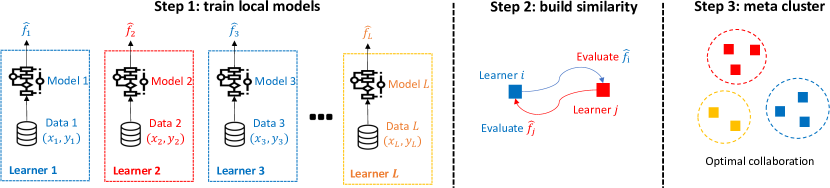
Figure 1: Illustration of meta clustering for learners/datasets, based on supervised relationships.

The general question of “how to collaborate” has led to several recent research on collaborative learning, which we will elaborate in Section 1.1. This paper aims to answer the following question: Whom to collaborate with? Selecting collaborators is crucial when not all learners are qualified, such as learners with incapable models or irrelevant sub-datasets. In particular, we suppose each sub-dataset is of a supervised nature, consisting of predictor-response pairs $(\bm{X},Y)$. A learner tends to collaborate with those whose data exhibit the same or similar underlying $\bm{X}$-$Y$ relationship. To that end, we propose to study the problem of clustering for supervised relationships. The idea is that sub-datasets exhibiting similar function relationships (between $\bm{X}$ and $Y$) should fall into the same cluster. An alternative view of such clustering is categorizing sub-datasets into fewer meta-datasets, offering better learning quality without inducing many estimation biases. As such, we name the problem “meta clustering.” Unlike the classical learning problem of data-level clustering, our goal here is to cluster datasets instead of single data points. In this framework, learners should collaborate with those in the same cluster. We focus on the regression scenario, where each sub-dataset can be modeled by $f(\bm{X})=E(Y|\bm{X})$ for some function $f$, and sub-datasets in the same cluster share the same (latent) function $f$. We propose a computationally efficient algorithm for meta clustering, consisting of three steps: select, exchange, and cluster. Figure 1 illustrates the main idea of the proposed method. In summary, we first train local models for each learner and select the best model. Then, each pair of learners exchange their already-learned best models. We then calculate the similarity between each pair of two learners by evaluating one’s model on the other’s dataset. Finally, spectral clustering is performed based on the similarity matrix.

The contribution of our work is three-fold. First, we propose to study the problem of clustering for datasets based on the underlying supervision relationships. The problem of meta clustering naturally fits the emerging need for robust collaborations in adversarial learning scenarios. We propose a general approach named Select-Exchange-Cluster (SEC). Second, the proposed SEC method is both computationally efficient and theoretically guaranteed. We show that when the sample size of each sub-dataset is sufficiently large, the sub-datasets with the same generating function can be accurately categorized into the same cluster. Moreover, the number of clusters does not need to be specified in advance, and it can be appropriately identified in a data-driven manner. Third, we can use the proposed method in general supervised regression tasks that involve non-linear and nonparametric learning models. It can be used for various learning tasks even if learners are not sure about the existence of latent functions. For example, we show its use to significantly enhance the prediction performance under data fairness constraints, where a reduction of approximated 50% prediction error is achieved without using any sensitive variable.

1.1 Related work

We briefly describe the connection between meta clustering and existing research.

Collaborative learning. When data are stored across distributed clients such as edge devices, directly sharing local datasets compromises data privacy. Federated learning (Konecny et al., 2016; McMahan et al., 2017; Ding et al., 2022) is a popular collaborative learning framework that aims to train a global model on distributed datasets without sharing local data. The main idea is to exchange model parameters updated from local data and iteratively update the globally trained model (assuming the same model for all clients). More general federated learning frameworks beyond exchanging parameters have been recently developed (Diao et al., 2021b, c). Our proposed meta clustering framework may serve as a preliminary analysis tool for selecting “qualified” collaborators before applying any federated learning algorithm. Assisted learning (Xian et al., 2020; Diao et al., 2021a, 2022) is another recently developed collaborative learning framework for decentralized organizations, where any organization being assisted or assisting others does not share its local data, model, or learning objective. In assisted learning, data variables held by participants are often distinct and assumed to be linked by a non-private identifier. In contrast, our paper focuses on the scenario where participants have the same variables, but the supervised relationships are possibly heterogeneous.

Data Integration. Data integration aims to improve statistical performance by sharing model parameters or combining datasets. Many methods have been proposed in this research direction. For example, Tang and Song (2016) developed a fused lasso approach to learn parameter heterogeneity in linear models on different datasets. Li and Li (2018) proposed an integrative method of linear discriminant analysis (LDA) for multi-type data, which was shown to improve classification accuracy over the performance on a single dataset. Jensen et al. (2007) proposed a Bayesian hierarchical model in a variable selection framework that integrates three types of data in gene regulatory networks: gene expression, ChIP binding, and promoter sequence. Yang et al. (2019) studied the problem of integrating regression data from different sources by pooling data for centralized learning. They proposed an objective function that estimates regression coefficients by penalizing pairwise differences between coefficients of the same covariate to identify heterogeneous and homogeneous coefficients automatically. Hector and Song (2020b) proposed a method for joint integrative analysis of multiple data sources with correlated vector outcomes under a distributed quadratic inference function framework. They assume the clustering of data sources is known. In that regard, our approach may be used as a preliminary step before applying their method when the underlying clustering structure is unknown.

In comparison with most data integration methods where statistical models are specified in each sub-dataset, our proposed meta clustering framework is model-free in the sense that it allows each learner to use different local models without sharing the form of those models. For example, one learner can use a linear model to fit a sub-dataset, while another can use a random forest. The proposed SEC algorithm only exchanges the predicted values for clustering without exchanging the parameters or the models. It is worth noting that with our meta clustering, a learner considers a binary decision whether to collaborate with another learner or not. A similar setup was also considered by Zhou et al. (2021), where the authors proposed the notion of model linkage selection for learners who share parameters of common interest. Alternatively, a learner may use a soft decision-based collaboration with others. In that direction, Shen et al. (2020) developed an approach that summarizes inference results from other learners as confidence density functions and then combines them using a weighting scheme. Tan et al. (2021) proposed a tree-based ensemble approach that integrates the prediction results from other learners as feature variables.

Divide-and-conquer. Divide-and-conquer in the context of distributed learning often refers to the procedure that partitions a large dataset into sub-datasets and then combines results (e.g., p-values, coefficients) obtained from each sub-dataset. For example, Zhang et al. (2015) proposed a method that randomly partitions the dataset into sub-datasets and fits a kernel ridge regression estimator in each sub-dataset. A simple average of local predictors is used as the global estimator, achieving minimax optimal convergence rates. Mackey et al. (2015) proposed the Divide-Factor-Combine (DFC) framework for noisy matrix factorization, which improves the scalability and enjoys estimation guarantees. Fan et al. (2019) proposed a distributed Principle Component Analysis (PCA) algorithm for data stored across multiple locations, which performs similarly to the PCA estimator based on the whole dataset. Different assumptions of the distributed sub-datasets were also investigated, such as independent cross-sectional data (Xie et al., 2011), independent sources/studies (Claggett et al., 2014; Battey et al., 2015), network meta-analysis (Yang et al., 2014), high-dimensional correlated data (Hector and Song, 2020a), and multi-measurements data from different experiments (Gao and Carroll, 2017).

The primary goal of divide-and-conquer is to reduce computational costs via parallel computing across sub-datasets. One learner may or may not have access to all the sub-datasets. In our framework, each learner can only access its local sub-dataset. Also, divide-and-conquer methods assume the underlying relationship between the response and the predictors for each sub-dataset is the same, so combining results from all the sub-datasets is reasonable. However, the datasets in distributed storage may be heterogeneous in distributions. Identifying the potential clustering of the subs-datasets is important for bias reduction and robust modeling. For divide-and-conquer methods, meta clustering can be applied to analyze whether there are potential cluster structures on the whole dataset. If there exist cluster structures, a random splitting in divide-and-conquer may lead to a modeling bias.

The remainder of the paper is outlined below. We describe the meta clustering problem in Section 2 and propose our method, together with its theoretical properties, in Section 3. In Section 4, we demonstrated a potential use of the method in fairness learning scenarios. In Sections 5 and 6, we show the performance of our method through more experimental studies. The proofs are included in the supplementary material.

2 Problem

Suppose the dataset $\mathcal{D}:=\{\mathcal{D}_{i}\}_{i=1}^{L}$ is the union of $L$ sub-datasets. For example, $\mathcal{D}_{i}$ can represent the sub-dataset stored in the $i$-th location/server, the sub-dataset from the $i$-th study in a meta-analysis, or the sub-dataset from the $i$-th patient in the same research project. We assume each sub-dataset $\mathcal{D}_{i}$ is handled by a learner $l_{i}$ who considers a set of available methods $\mathcal{M}_{i}=\mathcal{M}^{p}_{i}\cup\mathcal{M}^{non}_{i}$ for data analysis. Here $\mathcal{M}^{p}_{i}$ ($\mathcal{M}^{non}_{i}$) denotes the parametric (nonparametric) models in $\mathcal{M}_{i}$. Briefly speaking, we assume a parametric model (e.g., a linear regression model) has a better convergence rate than a nonparametric one (e.g., a decision tree), and the latter is consistent in estimation. More detailed assumptions are included in the supplementary document. The notions of parametric and nonparametric are made only for technical convenience. It is practically hard to distinguish them with finite samples, even in linear models. We refer to (Ding et al., 2018) for more discussions on this. Parallel computing can be regarded as a particular case when all sub-datasets use the same learner. Throughout the paper, we will use lowercase letters (e.g., $x$, $\bm{x}$, $a_{n}$) to denote observed data or constants, uppercase letters to denote random variables or vectors (e.g., $X$, $\bm{X}$), typewriter uppercase letters (e.g., $\mathtt{A}$) to represent matrices, and calligraphy uppercase letters (e.g., $\mathcal{A}$) to represent sets.

Suppose the sub-dataset $\mathcal{D}_{i}$ consists of $n_{i}$ independent data points, denoted by $\mathcal{D}_{i}=\{(y_{i,j},\bm{x}_{i,j}):y_{i,j}\in\mathbb{R},\bm{x}_{i,j}\in\mathbb{R}^{p}\}_{j=1}^{n_{i}}$, from the underlying model $Y_{i}=f_{i}(\bm{X}_{i})+{\varepsilon}_{i},$ where $\bm{X}_{1},\ldots,\bm{X}_{L}$ are independent $p$-dimensional random variables with a distribution function $P_{\bm{X}}(\cdot)$, and the noise ${\varepsilon}_{i}\sim\mathcal{N}(0,\sigma_{i}^{2})$ is independent of $\bm{X}_{i}$. Moreover, for any $i_{1},i_{2}\in\{1,\ldots,L\}$, ${\varepsilon}_{i_{1}}$ is independent of $\bm{X}_{i_{2}}$. We suppose the $L$ sub-datasets consist of the same $p$ predictors.

Let $n:=n_{1}+\cdots+n_{L}$ denote the overall sample size. Throughout the paper, we assume there are $K$ (fixed but unknown) data generating functions, namely $f_{i}\in\mathcal{F}=\{f^{(1)},\ldots,f^{(K)}\}$ for $i=1,\ldots,L$. Let $||\cdot||$ denote the Euclidean norm. Define the $L_{2}$ norm $\lVert f\rVert_{2}=\sqrt{\int f(\bm{x})^{2}P_{\bm{X}}(d\bm{x})}$ and the $L_{\infty}$ norm $||f||_{\infty}=\textrm{ess}\sup|f|=\inf\{c\geq 0:|f(\bm{X})|\leq c\ \textrm{a.s.}\}$. We say two underlying models $f^{(i)}$ and $f^{(j)}$ are different if $||f^{(i)}-f^{(j)}||_{\infty}>0$.

Our goal is to accurately cluster the $L$ sub-datasets into $K$ clusters, where the underlying regression functions corresponding to the sub-datasets in the same cluster are similar.

3 Method

The intuition of our method is that if two sub-datasets are from the same or similar data generating function, a modeling procedure should produce similar results on the two sub-datasets. We propose the following three-step method named Select-Exchange-Cluster (SEC), where learners communicate with their estimated regression functions.

Step 1 [Select]: Each learner uses its own sub-dataset to learn a model from a set of candidate methods $\mathcal{M}_{i}$. Suppose each learner conducts the half-half cross-validation to perform model selection. In particular, learner $l_{i}$ splits the data $D_{i}$ into two parts $\mathcal{D}_{i,1}$ and $\mathcal{D}_{i,2}$ of equal size $n_{i,1}=n_{i,2}=n_{i}/2$ (assuming an even $n_{i}$ for simplicity). The learner applies each candidate method $\delta\in\mathcal{M}_{i}$ to the training set $\mathcal{D}_{i,1}$ and obtains the corresponding estimator $\hat{\delta}_{n_{i,1}}$. For learner $l_{i}$, denote the best method $\delta_{i}$ as the one that minimizes the mean squared error (MSE) on the test set $\mathcal{D}_{i,2}$ , namely

$$\delta_{i}=\operatorname*{arg\,min}_{\delta\in\mathcal{M}_{i}}\sum_{(y,\bm{x})\in\mathcal{D}_{i,2}}\bigl{(}y-\hat{\delta}_{n_{i,1}}(\bm{x})\bigr{)}^{2}/n_{i,2}.$$ (1)

The “best” method $\delta_{i}$ is then applied to the whole data $\mathcal{D}_{i}$ to estimate the underlying function $f_{i}$. Denote the resulting estimated function as $\hat{f}_{{i}}$ and its fitted mean squared error as $\hat{e}_{i}:=\sum_{(y,\bm{x})\in\mathcal{D}_{i}}\bigl{(}y-\hat{f}_{{i}}(\bm{x})\bigr{)}^{2}/n_{i}.$ To summarize, for each learner $l_{i}$, we have the non-shared data $\mathcal{D}_{i}$ and the sharable information $\{\delta_{i},\hat{f}_{{i}},\hat{e}_{i}\}$.

Step 2 [Exchange]: For any two learners, they exchange the sharable information $\{\delta_{i},\hat{f}_{{i}},\hat{e}_{i}\}$. In particular, denote $v_{ij}$ as the dissimilarity between any two learners $(l_{i},l_{j})$, $i\neq j$. We apply the $i$-th learner’s best estimator $\hat{f}_{{i}}$ to the $j$-th learner’s dataset $\mathcal{D}_{j}$ and obtain its prediction loss $\hat{e}_{i\rightarrow j}:=n_{j}^{-1}\sum_{(y,\bm{x})\in\mathcal{D}_{j}}\bigl{(}y-\hat{f}_{{i}}(\bm{x})\bigr{)}^{2},$ where the subscript $i\rightarrow j$ denotes the information flow from $l_{i}$ to $l_{j}$. Similarly, we apply $\hat{f}_{{j}}$ to the dataset $\mathcal{D}_{i}$ and obtain the prediction loss $\hat{e}_{j\rightarrow i}$. The dissimilarity $v_{ij}$ is then defined as the difference between their best estimators:

$$v_{ij}=|\hat{e}_{i\rightarrow j}-\hat{e}_{j}|+|\hat{e}_{j\rightarrow i}-\hat{e}_{i}|,$$ (2)

where $v_{ij}=v_{ji}$ for any $i\neq j$. When $i=j$, the self-dissimilarity of a learner $l_{i}$ is $v_{ii}:=0$.

Step 3 [Cluster]: Based on the dissimilarity $v_{ij}$, a similarity matrix is constructed, which is used to cluster the $L$ learners. In particular, we calculate a symmetric matrix $\mathtt{S}$ whose $(i,j)$-th component is $\mathtt{S}_{ij}:=\exp(-av_{ij})$. Here, $a$ is a tuning parameter for computational convenience. For example, when $\min_{i,j}v_{ij}$ is large and $a=1$, $\mathtt{S}_{ij}$’s can be negligibly small for all $(i,j)$ and thus become not distinguishable by the computer (due to its limited precision). Let $\mathcal{P}=\{1,\ldots,L\}$ denote the set of labels of the $L$ learners. For a given $K$, we will find a collection of sets $\{\mathcal{S}_{i}\}_{i=1}^{K}$ that forms a partition of $\mathcal{P}$. The partition is obtained by applying a spectral clustering algorithm to the matrix $\mathtt{S}$ and dividing the $L$ learners into $K$ groups. For completeness, we summarize the clustering step (Step 3) in Algorithm 1.

Input: Number of learners $L$, learners/datasets {$\mathcal{D}_{i}\}_{i=1}^{L}$, the number of clusters $K$ (optional).

Output: The number of clusters $K$ (if not given), and the cluster labels $c_{i}\in\{1,\ldots,K\},i=1,\ldots,L$.

1. Calculate the similarity matrix $\mathtt{S}\in\mathbb{R}_{+}^{L\times L}$, where each $\mathtt{S}_{ij}=\exp(-av_{ij})$ and $v_{ij}$ is given by (2).

2. If $K$ is given, conduct the spectral clustering:

   1. Calculate the Laplacian $\mathtt{L}_{\mathtt{S}}$ of $\mathtt{S}$: $\mathtt{L}_{\mathtt{S}}=\mathtt{D}^{-1/2}\mathtt{S}\mathtt{D}^{-1/2}$, where $\mathtt{D}:=\text{diag}(\sum_{j=1}^{L}\mathtt{S}_{1j},\ldots,\sum_{j=1}^{L}\mathtt{S}_{Lj})$.

   2. Compute the $K$ largest eigenvectors of $\mathtt{L}_{\mathtt{S}}$: $\bm{u}_{1},\ldots,\bm{u}_{K}$. Denote $\mathtt{U}=[\bm{u}_{1},\ldots,\bm{u}_{K}]\in\mathbb{R}^{L\times K}$.

   3. Standardize each row of $\mathtt{U}$ to have unit $\ell_{2}$ norm. Denote the standardized matrix as $\mathtt{U}_{*}$.

   4. Apply k-means clustering to the rows of $\mathtt{U}_{*}$ into $K$ clusters, and record the labels $c_{i},i=1,\ldots,L$.

3. If $K$ is not given:

   1. Sort the eigenvalues of $\mathtt{S}$ from small to large and determine $K$ (Remark 2).

   2. Go back to Step 2.

Algorithm 1 Pseudocode for the Step 3 of SEC algorithm

Remark 1 (Spectral clustering).

There are different variants of spectral clustering in the literature. Due to technical convenience, we build on the work of (Ng et al., 2002). We will show that the spectral clustering algorithm based on the constructed similarity matrix can guarantee desirable performance.

Remark 2 (Selection of $K$).

When $K$ is unknown, we may add a penalty term $K\cdot\lambda_{n}$ in to the $k$-means clustering in Step 2(d) of Algorithm 1 to minimize

$$\sum_{t=1}^{K}\sum_{i,j\in\mathcal{S}_{t}}\frac{1}{2|\mathcal{S}_{t}|}||\mathbf{u}_{(i)}-\mathbf{u}_{(j)}||^{2}+K\cdot\lambda_{n}$$ (3)

over all possible partitions of $\mathcal{P}$ and a grid of values of $K$. Here, $\mathbf{u}_{(i)}$ denotes the $i$-th row of $\mathtt{U}_{*}$ defined in Algorithm 1. The minimization problem (3) is equivalent to comparing the within-cluster distance over a grid of $K$ values. We suggest $\lambda_{n}=O(\max(n^{-1},u^{4}_{n}))$, where $u_{n}$ is an upper bound of the convergence rates of non-parametric estimators (elaborated in the supplementary document). In practice, picking an appropriate penalty term may be complex because of the known convergence rates of nonparametric methods in Step 1. An alternative approach we suggest is using the gap statistics (Tibshirani et al., 2001) that searches for the so-called “elbow point” in the curve of the sum of within-cluster mean-squared errors (namely the first term in (3)) against different $K$’s. We will also show in the supplementary document that an adequately chosen penalty can select the correct $K$ with a high probability.

Remark 3 (Future prediction).

The clustering results may also be used for downstream collaborative learning methods, where a learner only interacts with others in the same cluster. Though prediction is not the main focus of this paper, we discuss two use cases to perform prediction based on the clustering results from SEC. For any particular learner $l_{i}$, suppose it belongs to the cluster $\mathcal{S}_{t}$. In the first case, the sub-datasets cannot be pooled due to communication bandwidths or privacy regulations. To collaborate, other learners in the same cluster may transmit their learned models $\hat{f}_{n_{j}}$ ($j\in\mathcal{S}_{t},j\neq i$) to the learner $l_{i}$. Then, to predict for a future observation $\bm{x}$, the learner $l_{i}$ uses the weighted average of the fitted models from learners in the same cluster, e.g.,

$$\sum_{i\in\mathcal{S}_{t}}\frac{n_{i}}{\sum_{j\in\mathcal{S}_{t}}n_{j}}\hat{f}_{{i}}(\bm{x}),$$ (4)

where the weights are proportional to the sample size. In this way, the above case does not require direct data-sharing among learners. It is worth mentioning that the weights in $\eqref{eq:futurepred}$ may not be optimal for a statistical gain of prediction accuracy. We include further discussions on the statistical gain in the supplementary material. The second use case is when the sub-datasets are allowed to be pooled. Then, the learner $l_{i}$ pools all the sub-datasets in a cluster $\mathcal{S}_{t}$ and fits one model to make future predictions. In this case, the learner $i$ directly obtains a larger sample and thus tends to learn a better model. Nevertheless, this case requires the learners to share data, which may violate the purpose of collaborative learning.

The following theorem shows that the SEC can accurately identify the correct clusters when the overall sample size goes to infinity. Its proof is included in the supplementary document.

Theorem 4.

Under some assumptions (elaborated in the supplementary document), the labels $c_{1},\ldots,c_{L}$ produced by SEC satisfy $c_{i}=c_{j}$ if and only if $f_{i}=f_{j}$, for any $i,j$, with probability going to one as $n\rightarrow\infty$.

Remark 5 (Data independence).

The clustering accuracy in the theorem may no longer hold if the independence of $y_{ij}$’s breaks down. For longitudinal settings, for example, we may assume additional conditions on $y_{ij}$ (e.g., a $\alpha$-mixing sequence) for the proof to hold. We leave the more sophisticated analysis for dependent data as future work.

4 Application to Data Fairness

One promising application of the proposed method is to enhance data fairness. Biases inherent in data collection and techniques based on these data will not address (sometimes even worsen) the inequity for disadvantaged groups. In recent years, there have been many works to define fairness, discover unfairness, and apply algorithms to promote fairness. For example, based on the maximum likelihood principle, Kamishima et al. (2011) proposed a prejudice remover regularizer (based on the mutual information between response and sensitive variables) for classification models. Hardt et al. (2016) proposed a criterion called equal opportunity (or equalized odds) for a particular sensitive variable and demonstrated how to adjust a predictor to alleviate discrimination. Zafar et al. (2017) devised a notion called positive rate disparity and proposed a method to reduce disparities in mistreatment and treatment. Verma and Rubin (2018) compared the differences among 20 fairness definitions for classification problems.

We consider a linear regression setting where the sensitive variable is independent of other variables. In particular, we generate a dataset $\mathcal{D}$ that consists of 50 sub-datasets $\{\mathcal{D}_{i}\}_{i=1}^{50}$, each with size $n_{i}=50$ from the linear model: $Y_{i}=X_{1i}+2X_{2i}-2X_{3i}+2X_{4i}+bR_{i}+\epsilon_{i}$, where $(X_{1i},X_{2i},X_{3i},X_{4i})\sim\mathcal{N}(0,\mathtt{I}_{4})$ are the non-sensitive variables, $\epsilon_{i}\sim\mathcal{N}(0,1)$ is the random noise, and $R_{i}$ is the sensitive variable that may induce unfairness if it were known. We consider different scales of the coefficient of the sensitive variable, $b\in\{0.01,0.5,1,2,3,4,5,6,20\}$. The sensitive variable $R_{i}$ is generated from a standard normal $\mathcal{N}(0,1)$ distribution and is set to be fixed for each given $i$. Using a fixed value as a sensitive variable is reasonable for data fairness problems where multiple measurements exist for the same subject. For example, if $\mathcal{D}$ represents longitudinal data and each sub-dataset represents a person, then the subject-specific sensitive variable (e.g., gender, race, age, home location) is fixed for each person. We set $R_{i}$ as a continuous variable in this example. We split the dataset into a training set of 30 sub-datasets (e.g., $\{\mathcal{D}_{i}\}_{i=1}^{30}$) and a test set of 20 sub-datasets (e.g., $\{\mathcal{D}_{i}\}_{i=31}^{50}$). For each learner in the test set, we further split it into two parts of the same size (e.g., $\mathcal{D}_{i}=\mathcal{D}_{i}^{1}\cup\mathcal{D}_{i}^{2}$). The splitting is because we need extra data points to cluster the learners in the test set. Then, the dataset $\mathcal{D}$ is reorganized into the following three sets: the training set $\{\mathcal{D}_{i}\}_{i=1}^{30}$, the test set $\{\mathcal{D}_{i}^{1}\}_{i=31}^{50}$, and the validation set $\{\mathcal{D}_{i}^{2}\}_{i=31}^{50}$.The random data splitting is repeated 100 times.

For the training set, in the existence of a sensitive variable, we consider three methods of building a model: Oracle, Fairness, SEC-Fairness. The Oracle method directly builds a linear regression model from the training set using the sensitive variable (namely without considering fairness constraints), which is expected to have the best predictive performance. The Fairness method builds a linear regression model on the training set without using the sensitive variable since using the sensitive variable is not allowed or even available in the modeling procedure. The SEC-Fairness method finds potential groupings among the sub-datasets in the training set before building models without the sensitive variable. In particular, it first uses the SEC algorithm on the training set to cluster these $30$ learners $\{\mathcal{D}_{i}\}_{i=1}^{30}$ into groups. Then, it uses the similarity between a learner and a cluster to identify which cluster (identified from the training set) each of these $20$ learners in the test set belongs to. To measure the similarity between a learner $l_{i}$ and a cluster, we use the sum of the similarities between $l_{i}$ with each learner in that cluster. Then, the learner $l_{i}$ belongs to a cluster if its similarity to the cluster is larger than any other cluster. In the SEC algorithm, for simplicity, each learner $l_{i}$ considers two candidate modeling methods: Random Forest (Breiman, 2001) (RF) and linear regression (LR), namely $\mathcal{M}_{i}=\{\textrm{RF},\textrm{LR}\}$ in the “select” step.

	SEC-Fairness		Fairness	Oracle
$b$	MSE	$\hat{K}$	MSE	MSE
0.01	1.03 (0.005)	1 (0)	1.03 (0.005)	1.03 (0.005)
0.5	1.12 (0.007)	2.25 (0.59)	1.20 (0.007)	1.03 (0.005)
1	1.41 (0.02)	2.65 (0.59)	2.04 (0.03)	0.92 (0.005)
2	1.96 (0.04)	2.64 (0.48)	5.19 (0.09)	1.06 (0.005)
3	4.31 (0.22)	2.77 (0.44)	12.55 (0.27)	0.96 (0.005)
4	4.79 (0.28)	2.86 (0.37)	15.16 (0.36)	1.00 (0.005)
5	4.21 (0.12)	2.97 (0.17)	18.89 (0.36)	0.99 (0.005)
6	12.03 (0.60)	2.81 (0.39)	50.58 (1.04)	1.06 (0.004)
20	80.47 (4.90)	2.91 (0.29)	438.64 (9.38)	1.07 (0.006)

Table 1: Predictive performances of the three methods for the data fairness example. (The values in the parentheses are the standard error of the averaged MSE and the standard deviation of the estimated number of clusters $\hat{K}$ respectively over $100$ replications.)

For the validation set, we evaluate the predictive performances of the models by the mean square error (MSE), which are presented in Table 1. As shown in the table, when the importance (coefficient $b$) of the sensitive variable is high, the SEC-Fairness reduces the MSE of Fairness by about 50% overall. One possible reason is as follows. The linear relationship between $y$ and the variables $\{X_{1},\ldots,X_{4}\}$ only differs in the intercept per learner. The similarity between two learners, as in the SEC algorithm, will be small if the difference between their sensitive variables $|R_{i}-R_{j}|$ is large. It is then more likely that SEC divides those with similar values of the sensitive variable into the same cluster. It is worth mentioning that the SEC-fairness method satisfies the fairness constraint since it does not utilize the sensitive variable at all, and the non-sensitive variables used for clustering are independent of the sensitive variable.

The Oracle method, as expected, is very stable in MSE (around 1) over different values of $b$. When $b$ is large, SEC-Fairness is comparable to the oracle method, though it performs better than the Fairness method. One reason is that the estimated number of clusters $\hat{K}$ is in the interval $[2,3]$. In this example, we select $\hat{K}$ by the gap statistic. We note that there exists no “true” value of $K$ since every learner/sub-dataset has a unique sensitive value. In the case $b=20$, we have $\hat{K}=2.91$. But if we force $\hat{K}=10$ in the SEC algorithm, the MSE performance of SEC-Fairness is much improved. One reason that the gap statistic selects a small $\hat{K}$ is that it chooses the value of $K$ that most reduces the gap compared with $K-1$ instead of selecting $K$ that achieves the global minimum. Consequently, the gap statistic tends to select $\hat{K}$ as 3 or 4 in this example. An alternative way to estimate $K$ is cross-validation. Specifically, we can split each sub-dataset into a training set and a test set. Then, on the collection of the test sets, we can compare the MSE performance based on a list of $K$’s and select the most appropriate $K$. The cross-validation splitting ratio for each sub-dataset will likely affect the selection of $K$. We recommend using half-half splitting for each sub-dataset. Because the sample size $n_{i}$, the modeling methods $\mathcal{M}_{i}$, and the existence of data heterogeneity are different across learners, it will be nontrivial and interesting to study how to decide the splitting ratios of cross-validation. We leave that as future work and refer interested readers to (Ding et al., 2018; Zhang et al., 2022) for related discussions on cross-validation.

5 Simulated Data Experiments

In this section, we present two simulation settings. Each example is repeated $100$ times. From a theoretical view, no standardization of the data is required since only the function relationship between $Y$ and $\bm{X}$ matters. So one cluster may contain two sub-datasets/learners whose responses or predictors are not on the same scale. However, the nonparametric method usually requires compact support, which may cause some computational issues. In the experiments, we standardize $\bm{x}$ and $y$ in each sub-dataset/learner.

5.1 Simulation 1: clustering accuracy

This example is to demonstrate the clustering accuracy of our method. A clustering result is accurate if the number of clusters is accurately identified, and each learner’s label matches the underlying truth (up to a permutation). Suppose there are $20$ learners, $\{l_{i}\}_{i=1}^{20}$, each with a sub-dataset $D_{i}$ containing $n_{i}=50$ observations and $p=5,10,20$ predictors. The data of the first ten learners are generated from the underlying model $Y=f_{1}(\bm{X})+{\varepsilon}_{1}=\bm{\beta}_{1}^{{\mathrm{\scriptscriptstyle T}}}\bm{X}+{\varepsilon}_{1}$, where $\bm{X}\sim\mathcal{N}(0,\mathtt{I}_{p})$, ${\varepsilon}_{1}\sim\mathcal{N}(0,\sigma^{2})$, and $\bm{\beta}_{1}\in\mathbb{R}^{p}$. The data of the remaining 10 learners are generated from $Y=f_{2}(\bm{X})+{\varepsilon}_{2}=\bm{\beta}_{2}^{{\mathrm{\scriptscriptstyle T}}}\bm{X}+{\varepsilon}_{2}$, with ${\varepsilon}_{2}\sim\mathcal{N}(0,\sigma^{2})$, and $\bm{\beta}_{2}\in\mathbb{R}^{p}$. We randomly generate $\bm{\beta}_{1}$ and $\bm{\beta}_{2}$ from the standard Gaussian distribution (both $\bm{\beta}_{1}$ and $\bm{\beta}_{2}$ are set as fixed in each replicated experiment such that $\bm{\beta}_{1}\neq\bm{\beta}_{2}$). The signal-to-noise ratio (SNR) is defined by $\mathbb{E}(\|\bm{\beta}\|^{2})/\mathbb{E}({\varepsilon}^{2})$, which reduces to $p^{2}/\sigma^{2}$ in this case. We set the SNR level to be one of the following: $2^{0},\ldots,2^{7}$, and the corresponding noise level $\sigma^{2}=p^{2}/\textnormal{SNR}$ falls into the range of $25/128$ to $400$. In the SEC algorithm, let each learner consider two candidate methods: LASSO (Tibshirani, 1996), with built-in half-half cross-validation to select the tuning parameter, and Random Forest, with 50 trees and depth 3. We apply the SEC algorithm to cluster the 20 sub-datasets. The averaged clustering accuracy over $100$ replications is presented in Figure 2. We can see that the clustering accuracy increases as the SNR increases. Also, for a fixed SNR, a smaller $p$ tends to lead to better clustering accuracy. It is mainly because a less parsimonious model suffers from more estimation variance given the same amount of data. We also see that for a fixed $p$, the accuracy curve tends to be flat when SNR is larger than $2^{5}$, showing the SEC algorithm’s robustness against high noise levels. In Figure 3, we also present the result of a replication of the simulation with $p=5$ and SNR$=2^{4}$, with clustering accuracy near $100\%$. The eigenvalues used to apply the gap statistic are plotted in Figure 3(a). The eigenvectors in the spectral clustering algorithm are shown in Figure 3(b).

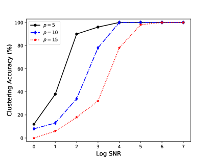
Figure 2: Clustering accuracy of the SEC algorithm for Simulation 1.

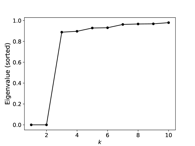
(a) Eigenvalues used to determine the gap statistic and number of clusters.

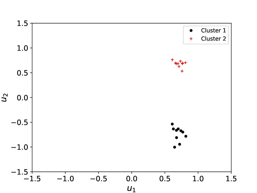
(b) Eigenvectors of the learners, indicated by the underlying true labels.

Figure 3: An illustration of the clustering results for Simulation 1, based on a realization with $p=5$, SNR=$2^{4}$.

5.2 Simulation 2: robustness against candidate models

In this example, we demonstrate that our method is robust against candidate models in the cross-validation part of the “select” step. Suppose there are $20$ learners, $\{l_{i}\}_{i=1}^{20}$, each with a sub-dataset $D_{i}$ containing $n_{i}=100$ observations and $p=500$ predictors. We use the following two benchmark datasets described in (Friedman, 1991; Breiman, 1996). The sub-datasets of the first ten learners are generated from $Y=f_{1}(\bm{X})+{\varepsilon}_{1}=\sqrt{X_{1}^{2}+(X_{2}X_{3}-1/(X_{2}X_{4}))^{2}}+{\varepsilon}_{1},$ and the sub-datasets of the remaining ten learners are generated from $Y=f_{2}(\bm{X})+{\varepsilon}_{2}=\arctan(X_{2}X_{3}-1/(X_{2}X_{4})/X_{1}+{\varepsilon}_{2},$ where $X_{1}\sim U(0,100)$, $X_{2}\sim U(40\pi,560\pi)$, $X_{3}\sim U(0,1)$, $X_{4}\sim U(1,11)$, and ${\varepsilon}_{1},{\varepsilon}_{2}\sim\mathcal{N}(0,0.01)$ are independent. The remaining 496 predictors $\{X_{5},\ldots,X_{500}\}$ follow a standard multivariate gaussian distribution $\mathcal{N}(0,\mathtt{I}_{496})$.

For each learner, we consider the candidate methods: Random Forest (RF), k-nearest neighbors (KNN), Support Vector Regression (SVR) (Drucker et al., 1997), Neural Network (NN), Gradient Boosting (Friedman, 2001) (GB), LASSO, Least Angler Regression (Efron et al., 2004)(LARS), Elastic Net(Zou and Hastie, 2005) (EN), Ridge Regression (Ridge). To show the robustness of our procedure against the number of candidate models and against the types of candidate models, we consider four different choices of $\mathcal{M}_{i}$: {RF, KNN, SVR, NN, GB, LASSO, LARS, EN, Ridge}, $\{\textrm{RF},\textrm{KNN},\textrm{SVR},\textrm{GB},\textrm{LASSO},\allowbreak\textrm{LARS},\textrm{EN}\}$, $\{\textrm{RF, KNN, GB, LASSO, LARS}\}$, $\{\textrm{RF, GB, LASSO}\}$, and $\{\textrm{GB}\}$. The results are presented in Table 2. The clustering accuracy is stable over different choices of $\mathcal{M}_{i}$. We can see the robustness of our method against both the number of candidate models and the type of candidate models.

$|\mathcal{M}{}_{i}|$	Proportion being selected	Accuracy	$\hat{K}$	Collaboration	No collaboration
	(GB, RF, LASSO)			MSE	MSE
1	(1, 0, 0)	66.0	2	0.100(0.0056)	0.133(0.0038)
3	(0.56, 0.11, 0.33)	74.0	2	0.095(0.0053)	0.131(0.0042)
5	(0.56, 0.10, 0.34)	58.0	2	0.087(0.0049)	0.125(0.0044)
7	(0.57, 0.11,0.32)	70.0	2	0.096(0.0056)	0.134(0.0051)
9	(0.57, 0.10, 0.33)	64.0	2	0.060(0.0018)	0.112(0.0034)

Table 2: Prediction performance with collaboration and without collaboration, under various sets of candidate methods (rows). The column “Proportion being selected” is the proportion of each method being selected as the best method. The column “Accuracy” is the clustering accuracy of the SEC algorithm. The standard error of the averaged MSE over $100$ replications is reported in parentheses. The $\hat{K}$ denotes the estimated number of clusters.

Without loss of generality, we focus on the first learner $l_{1}$ to evaluate whether the SEC algorithm improves prediction accuracy. We generate a test set $\mathcal{D}_{\textrm{test}}=\{(y_{i}^{\textrm{test}},\bm{x}_{i}^{\textrm{test}})\}^{100}_{i=1}$ generated from the model $Y=f_{1}(\bm{X})+{\varepsilon}_{1}$. We consider two modeling methods: No collaboration and Collaboration. The “Collaboration” method first applies the SEC algorithm and identifies learners in the same cluster as $l_{1}$. Then, we obtain the prediction for the test set $\mathcal{D}_{\textrm{test}}$ based on the simple average of the estimated predictors from those learners, as described in the formula (4). The “No Collaboration” method simply fits $l_{1}$’s favored method on its own sub-dataset $\mathcal{D}_{1}$ and applies the estimator on the test set $\mathcal{D}_{\textrm{test}}$ to make predictions. The mean squared errors of the above two methods’ predictions are also shown in Table 2. Overall, “Collaboration” has a smaller MSE than “No Collaboration.” For $|\mathcal{M}_{i}|=1$, a right-sided t-test of the MSE’s of “No Collaboration” to that of “Collaboration” produces a p-value of $2.1\times 10^{-6}$. We also observe significantly small p-values for other cases of $|\mathcal{M}_{i}|$. When the number of candidate models in $\mathcal{M}_{i}$ is larger, the MSE of the “Collaboration” method is smaller. The above is because more candidate models in the cross-validation part of the “select” step enable us to understand better the function relationship between the response and the predictors so that the similarity matrix can better capture the true underlying clusters. The prediction accuracy of the two methods is also stable across different choices of $\mathcal{M}_{i}$, in terms of both the size of $\mathcal{M}_{i}$, $|\mathcal{M}_{i}|$ and the methods in $\mathcal{M}_{i}$.

6 Real Data Applications

In this section, we apply the SEC algorithm in two real data examples.

6.1 Application 1: CT Image Data

We investigate the CT Image dataset in (Graf et al., 2011) that consists of $53500$ CT slices and $385$ variables. These $53500$ CT slices are obtained from $97$ CT scans, where $74$ patients ($43$ male and $31$ female) took at most a thorax scan and a neck scan. The response variable is the relative location of the CT slice on the axial axis. The relative location of the CT slice on the axial axis is critical for registering CT scans in a body atlas (Graf et al., 2011), which enables the comparison of different CT scans. This dataset has a natural sub-dataset structure since many CT slices are from the same CT scan that can be treated as a sub-dataset.

We divide the dataset into $97$ sub-dataset/learners, each containing all the CT slices from a single CT scan. Our goal is to find any potential clustering structure (and the corresponding variable) that improves both scientific understanding and predictive performance. We randomly divide these $97$ learners into two parts: the training set ($64$ learners) and the test set ($33$ learners). Similar to the data fairness example, for each of the $33$ learners in the test set, we divide the sub-dataset into two sets of equal size.

For the training set, we consider three methods: “clustering (pooled)”, “clustering (unpooled)”, and “no clustering”. The “no clustering” method directly trains a Random Forest model on the training set. The “clustering (pooled)” method first applies the SEC algorithm to classify the learner in the training set into clusters, with $\mathcal{M}_{i}=\{\textrm{RF},\textrm{LASSO}\}$ for $i=1,\ldots,64$. Then it trains a Random Forest model separately in each identified cluster (with all the within-cluster sub-datasets pooled). In contrast, the “clustering (unpooled)” does not pool the sub-datasets in the cluster but trains a Random Forest in each sub-dataset. For sub-datasets/learners in the validation set, the ‘no clustering’ method directly applies the trained random forest model to all the learners and obtains the overall mean squared error. The “clustering (pooled)” method first determines to cluster each learner belongs to and then applies the cluster-level trained random forest model. In contrast, the “clustering (unpooled)” method applied a weighted average as in equation (4). We repeat the data splitting $100$ times and summarize the results in Table 3. The results show that both options (unpooled and pooled) can significantly outperform that of the “no clustering” method. A right-sided paired t-test that compares the MSE of “clustering (unpooled)” and “clustering (pooled)” with that of “no clustering” produces p-values of $1.43\times 10^{-13}$ and $1.77\times 10^{-14}$, respectively. The “clustering (unpooled)” improves the MSE by 31$\%$ than “no clustering”, and the “clustering (unpooled)” has a slightly worse MSE compared with “clustering (pooled)”. This demonstrates the promising performance of collaborative learning even without pooling data.

	Clustering (pooled)	Clustering (unpooled)	No Clustering
MSE	94.09 (4.18)	103.07(3.79)	150.52 (2.10)
$\hat{K}$	2 (6 times) and 3 (94 times)		N/A

Table 3: Results for the CT Image Data. The value in the parenthesis is the standard error of the averaged MSE over $100$ replications, and $\hat{K}$ denotes the estimated clusters.

We also looked for a scientific understanding of the identified clusters on the training set. So we investigated possible variables related to the cluster structure discovered by the SEC. Unfortunately, either the gender of the patient or whether the CT scan is from the thorax or neck is not available in the dataset (Graf et al., 2011). However, this example does show the possibility of finding essential variables related to the cluster structure if further information is provided. Additionally, we can significantly improve the predictive performance without assessing any patient private information but the CT images themselves.

6.2 Application 2: Electrical Grid Stability Data

This example is to demonstrate the performance of the SEC algorithm when the data are under adversarial attacks. The Electrical Grid Stability Data (Arzamasov et al., 2018) consists of 10000 observations and $14$ variables. Among the $14$ variables, two variables describe the system stability: one is categorical (stable/unstable), and the other is continuous (a positive value means a linearly unstable system). We use the continuous variable as the response. The other $12$ variables are the input of the Decentral Smart Grid Control system.

We first divide the data into training set ($n_{1}=8000$) and the test set ($n_{2}=2000$). The training set is randomly divided into $50$ learners, each with $160$ observations. We may assume the data are stored in $50$ servers, and some servers get attacked by hackers. Let $d=0,1,\ldots,49$ denote the number of attacked learners. We set that the first $d$ out of $50$ learners are attacked. Each time a sub-dataset is “attacked,” we change the response variable to the negative of its original value. We also assume that the $50$th learner knows that its dataset is not attacked.

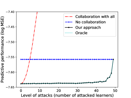
Figure 4: Prediction error (evaluated by MSE) as an increasing function of attack severity.

Under potential attacks, we consider four options of the 50th learner to perform data analysis, denoted as “Collaboration with all”, “No collaboration”, “Our approach”, and “Oracle”. The “Collaboration with all” option ignores the fact that some learners/sub-datasets are attacked and insist on collaborating with all the other learners. In the “No collaboration” option, a learner (say the 50th) trusts nobody but itself and uses its sub-dataset for learning. In the “Our approach” option, the 50 learners are clustered by SEC into “attacked” and “intact”. Then the learners classified as intact will collaborate. The “Oracle” option means that an oracle knows which learners are attacked and collaborates with those intact ones. In collaboration, we allow the learners to share datasets. In other words, once a learner identifies collaborators, the learner pools the data and fits a linear regression.

The trained linear model is then applied to the test set to evaluate its performance (MSE). We plot the predictive performance against the number of attacked learners in Figure 4. We only present part of the red curve since it explodes as the level of attacks increases. The value of the red curve increases from $-7.65$ to $-5.25$ when the number of attacked learners increases from $0$ to $49.$ As the proposed method accurately clusters all the intact learners, the performance curve of “Our approach” overlaps with that of “Oracle”. We also see that the predictive performance of “Our approach” decreases when the level of attack (meaning the number of the attacked learners) increases. In particular, the decrease becomes very sharp when the number of attacked learners is greater than $45$. One reason is that the linear model based on the information of one sub-dataset (with a sample size of $160$ and $12$ predictors) or two is enough to capture the underlying relationship. Indeed, the scale of MSE is very small ($10^{-4}$). So collaborating with more than five intact learners may not improve the prediction accuracy much compared with collaborating with only two intact learners.

The proposed SEC algorithm can be applied even though each learner can only access its own sub-dataset. Nevertheless, the SEC algorithm can be applied when each learner has access to all the sub-datasets. In such cases, we envision it as a pre-screening method to screen out contaminated sub-datasets, which improves modeling and prediction accuracy.

7 Conclusion

This paper proposed a framework of meta clustering for selecting “qualified” collaborators for collaborative learning. If two datasets exhibit a similar underlying relationship between the response and predictors, they fall in the same cluster. We developed a clustering algorithm named SEC to perform meta clustering efficiently. It only requires the exchange of fitted functions instead of raw data to evaluate the similarity among datasets. We showed promising applications of the framework to enhance data fairness, improve single-learner prediction accuracy, and discover potential grouping structures of a dataset.

Appendix

Appendix A Technical proofs

A.1 Notation

For a sequence of random variables $\{X_{n}\}$ and a deterministic sequence $\{a_{n}\}$, $n=1,2,\ldots$, we write $X_{n}\lesssim a_{n}$ if $X_{n}=O_{p}(a_{n})$. We write $X_{n}\gtrsim a_{n}$ if for any constant $\delta\in(0,1)$ there exists a $c_{\delta}>0$ such that $\liminf_{n\rightarrow\infty}\mathbb{P}(X_{n}\geq c_{\delta}a_{n})\geq 1-\delta$. If both $X_{n}\lesssim a_{n}$ and $X_{n}\gtrsim a_{n}$, we then write $X_{n}\sim a_{n}$.

An estimator $\{\hat{f}_{n}\}_{n=1}^{\infty}$ is said to converge in probability to $f$ at the rate $\{a_{n}\}$ if $\lVert\hat{f}_{n}-f\rVert_{2}\sim a_{n}$. We use the notation $\delta_{f}$ to denote the modeling method that corresponds to the data generating function $f$. For example, let $f(\bm{x})=x_{1}+x_{2}+x_{3}$ and then we can denote the linear regression of the response on the variables $\{x_{1},x_{2},x_{3}\}$ as $\delta_{f}$.

A.2 Assumptions

Assumption 1.

The number of learners $L$ is a fixed positive integer. For each $n_{i}$, $i=1,\ldots,L$, $n_{i}\sim n$ as $n\rightarrow\infty$ where $n=n_{1}+\cdots+n_{L}$.

Assumption 2.

For each $f_{i}$ and its estimator $\hat{\delta}_{i}\in\mathcal{M}_{i}$ from $\mathcal{D}_{i}$, $\exists\ M_{1}>0$ such that $||f_{i}(x)-\hat{f}_{i}(x)||_{\infty}<M_{1}$, $\forall\ n\geq 1$.

Assumption 3.

We assume that each learner uses at least one nonparametric modeling method: $\mathcal{M}^{non}_{i}\neq\emptyset$, $\forall\ i=1,\ldots,L$.

Assumption 4.

There exists sequences $\{\ell_{n}\}$ and $\{u_{n}\}$ such that

$$\sqrt{n}\min\{\ell_{n},u_{n}\}\rightarrow\infty\textrm{ as }n\rightarrow\infty.$$ (5)

$$\max\{\ell_{n},u_{n}\}\rightarrow 0\textrm{ as }n\rightarrow\infty,$$ (6)

and that for each $i=1,\ldots,L$, for any nonparametric estimator $\hat{f}_{n_{i}}\in\mathcal{M}^{non}_{i}$,

$$\ell_{n_{i}}\lesssim\lVert f_{i}-\hat{f}_{n_{i}}\rVert_{2}\lesssim u_{n_{i}}.$$ (7)

Moreover, for each $i=1,\ldots,L$, for any parametric estimator $\hat{f}_{n_{i}}=f_{\hat{\theta}_{n_{i}}}\in\mathcal{M}^{p}_{i}$,

$$\lVert f_{i}-\hat{f}_{n_{i}}\rVert_{2}\sim n_{i}^{-1/2}\qquad \textrm{ if }f_{i}\in\{f_{\theta}:\theta\in\Theta_{i}\}$$ (8)

$$\lVert f_{i}-\hat{f}_{n_{i}}\rVert_{2}\sim 1\qquad \textrm{ if }f_{i}\not\in\{f_{\theta}:\theta\in\Theta_{i}\}.$$ (9)

Assumption 5.

The difference between any two functions $\Delta f_{i,j}=f_{j}-f_{i}$ is bounded, i.e., $||\Delta f_{i,j}||_{\infty}<\infty$

Assumption 6.

The underlying functions $f^{(i)}$ are bounded, i.e., $||f^{(i)}||_{\infty}<\infty$.

Assumption 4 says that all the nonparametric methods will be consistent in estimating the underlying regression function (in the sense of $L_{2}$ distance). When the model class $\mathcal{M}^{p}$ includes the data generating regression function, namely the data generating model is parametric, the correct parametric models will converge to the truth at a parametric (which is the square root of sample size), faster than nonparametric rates. However, when $\mathcal{M}^{p}$ does not include the underlying regression function, then the estimation error will be bounded away from zero in probability. This assumption is very mild and common in regression analysis. More detailed discussions could be found in, e.g., (lu2019assessing) and the reference therein.

A.3 Proof of Theorem 4

To prove the theorem, we first prove the following three lemmas, which provide theoretical guarantees of the SEC algorithm’s three steps.

A.3.1 Step 1

In the following lemma we show that the cross-validation in Step 1 will select the correct one if the underlying function is parametric and specified in the candidate methods. Otherwise, nonparametric methods are favored.

Lemma 1.

Assume Assumptions 2, 3 and 4 hold. For each learner $l_{i}$, if the corresponding modeling method of the underlying data generating function is specified in the candidate models, namely $\delta_{f_{i}}\in\mathcal{M}_{i}^{p}$, then the $\delta_{f_{i}}$ will be selected by the cross-validation in step 1 with probability going to one as $n\rightarrow\infty$. Otherwise, there exists a method $\delta^{\prime}\in\mathcal{M}_{i}^{non}$ that minimizes the cross-validation error (equation (2) in the article).

Proof.

For any candidate modeling method $\delta\in\mathcal{M}_{i}$, denote its corresponding estimator as $\hat{\delta}_{n_{i}/2}$ where the subscript denotes that the estimator is obtained from the training set with sample size $n_{i}/2$. The cross-validation error of the method $\delta$ is

$$e(\hat{\delta}_{n_{i}/2}): =\frac{2}{n_{i}}\sum_{t=n_{i}/2+1}^{n_{i}}\bigl{(}f_{i}(\bm{x}_{t})+{\varepsilon}_{it}-\hat{\delta}_{n_{i}/2}(\bm{x}_{t})\bigr{)}^{2}$$

$$=\frac{2}{n_{i}}\sum_{t=n_{i}/2+1}^{n_{i}}\bigl{(}f_{i}(\bm{x}_{t})-\hat{\delta}_{n_{i}/2}(\bm{x}_{t})\bigr{)}^{2}+\frac{2}{n_{i}}\sum_{t=n_{i}/2+1}^{n_{i}}{\varepsilon}_{it}^{2}$$

$$\quad+\frac{4}{n_{i}}\sum_{t=n_{i}/2+1}^{n_{i}}\bigl{(}f_{i}(\bm{x}_{t})-\hat{\delta}_{n_{i}/2}(\bm{x}_{t})\bigr{)}{\varepsilon}_{it}.$$

For a sequence $\{X_{n}\}$ where each element has a finite variance, we have $X_{n}-E(X_{n})=O_{p}(\sqrt{\textrm{Var}(X_{n})})$. So we have $\frac{2}{n_{i}}\sum_{t=n_{i}/2+1}^{n_{i}}{\varepsilon}_{it}^{2}=\sigma_{i}^{2}+O_{p}(n_{i}^{-1/2})$. By Assumption 2, we have

$$\frac{4}{n_{i}}\sum_{t=n_{i}/2+1}^{n_{i}}\bigl{(}f_{i}(\bm{x}_{t})-\hat{\delta}_{n_{i}/2}(\bm{x}_{t})\bigr{)}{\varepsilon}_{it}=O_{p}(n_{i}^{-1/2})$$

and

$$\frac{2}{n_{i}}\sum_{t=n_{i}/2+1}^{n_{i}}\bigl{(}f_{i}(\bm{x}_{t})-\hat{\delta}_{n_{i}/2}(\bm{x}_{t})\bigr{)}^{2}=\lVert f-\hat{\delta}_{n_{i}/2}\rVert^{2}+O_{p}(n_{i}^{-1/2}).$$

Together with Assumption 4, we have $e(\hat{\delta}_{n_{i}/2})=\lVert f-\hat{\delta}_{n_{i}/2}\rVert^{2}+\sigma_{i}^{2}+O_{p}(n_{i}^{-1/2})\sim\sigma_{i}^{2}+O_{p}(\max\{n_{i}^{-1/2},u_{n_{i}}^{2}\})$.

If $f_{i}$ is a parametric model and the corresponding modeling method is contained in $\mathcal{M}_{i}^{p}$, then by Assumption 4,

$$\lVert f-\hat{\delta}_{n_{i}/2}\rVert^{2}+\sigma_{i}^{2}+O_{p}(n_{i}^{-1/2})\sim\sigma_{i}^{2}+O_{p}(n_{i}^{-1/2})$$

for a parametric $\hat{\delta}_{i}$ and

$$\lVert f-\hat{\delta}_{n_{i}/2}\rVert^{2}+\sigma_{i}^{2}+O_{p}(n_{i}^{-1/2})\sim\sigma_{i}^{2}+O_{p}(\max\{n_{i}^{-1/2},u_{n_{i}}^{2}\})$$

for a nonparametric $\hat{\delta}_{i}$. So if the $u_{n}\succ n^{-1/4}$, the selection process will pick the correct parametric model $\delta$.

If $f_{i}$ is a parametric model and the corresponding modeling method is not contained in $\mathcal{M}_{i}^{p}$, or $f_{i}$ is a nonparametric model, we have $\lVert f-\hat{\delta}_{n_{i}/2}\rVert^{2}+\sigma_{i}^{2}+O_{p}(n_{i}^{-1/2})\sim\sigma_{i}^{2}+1$ for parametric $\delta$ and $\sim\sigma_{i}^{2}+O_{p}(\max\{n_{i}^{-1/2},u_{n_{i}}^{2}\})$ for a nonparametric $\delta$. Thus, nonparametric models will be favored. ∎

A.3.2 Step 2

The following lemma states that the dissimilarity $v_{ij}$ constructed in the Exchange step has a well-separation property.

Lemma 2.

Assume Assumptions 2, 3, 4,and 5 hold. If $i,j$ are in the same cluster, namely $f_{i}=f_{j}$, we have $v_{ij}=o_{p}(1)$ as $n\rightarrow\infty$. Otherwise, we have $v_{ij}=||f_{i}-f_{j}||_{2}^{2}+||\Delta f_{i,j}||_{1}E||f_{j}-\hat{f}_{n_{i}}||_{1}+o_{p}(1)$, namely bounded away from 0 in probability.

Proof.

Suppose the fitted model $\hat{f}_{n_{i}}$ from learner $i$ is applied to data $\mathcal{D}_{j}$. Let $\mathbb{E}_{n_{j}}g=n_{j}^{-1}\sum_{t=1}^{n_{j}}g(\bm{x}_{t})$ be the empirical expectation for any measurable function $g(\cdot)$. Let $\Delta f_{i,j}=f_{j}-f_{i}$. Then the quadratic loss $\hat{e}_{i\rightarrow j}$ satisfies

$$\hat{e}_{i\rightarrow j} =\mathbb{E}_{n_{j}}\bigl{(}f_{j}-\hat{f}_{n_{i}}+{\varepsilon}_{j}\bigr{)}^{2}$$

$$=\mathbb{E}_{n_{j}}\bigl{(}\Delta f_{i,j}\bigr{)}^{2}+\mathbb{E}_{n_{j}}{\varepsilon}_{j}^{2}+\mathbb{E}_{n_{j}}\bigl{(}f_{i}-\hat{f}_{n_{i}}\bigr{)}^{2}+2\mathbb{E}_{n_{j}}\{\Delta f_{i,j}\bigl{(}f_{i}-\hat{f}_{n_{i}}\bigr{)}\}+2\mathbb{E}_{n_{j}}\bigl{(}f_{j}-\hat{f}_{n_{i}}\bigr{)}\cdot{\varepsilon}_{j}$$

$$\quad+2\mathbb{E}_{n_{j}}\Delta f_{i,j}\cdot{\varepsilon}_{j}.$$

By Assumptions 2 and 5, we have

$$2\mathbb{E}_{n_{j}}\{\Delta f_{i,j}\bigl{(}f_{i}-\hat{f}_{n_{i}}\bigr{)}\}+2\mathbb{E}_{n_{j}}\bigl{(}f_{j}-\hat{f}_{n_{i}}\bigr{)}\cdot{\varepsilon}_{j}+2\mathbb{E}_{n_{j}}\Delta f_{i,j}\cdot{\varepsilon}_{j}=||\Delta f_{i,j}||_{1}E||f_{j}-\hat{f}_{n_{i}}||_{1}+O_{p}(n_{j}^{-1/2}).$$

By Assumption 3, $\hat{f}_{j}$ is at least consistent in estimating $f_{j}$ at a nonparametric rate. Thus we have

$$\hat{e}_{i\rightarrow j}=||\Delta f_{i,j}||_{2}^{2}+\mathbb{E}_{n_{j}}{\varepsilon}_{j}^{2}+O_{p}(u_{n_{i}}^{2})+O_{p}(n_{j}^{-1/2}).$$ (10)

Similar arguments lead to

$$\hat{e}_{j}=\mathbb{E}_{n_{j}}{\varepsilon}_{j}^{2}+\Delta f_{i,j}E||f_{j}-\hat{f}_{n_{i}}||_{1}+O_{p}(u_{n_{j}}^{2})+O_{p}(n_{j}^{-1/2}).$$ (11)

Therefore, $\hat{e}_{i\rightarrow j}-\hat{e}_{j}=o_{p}(1)$ if $f_{i}=f_{j}$, and otherwise $v_{ij}=||f_{i}-f_{j}||_{2}^{2}+||\Delta f_{i,j}||_{1}E||f_{j}-\hat{f}_{n_{i}}||_{1}+o_{p}(1)$.

∎

Remark 6.

Theoretically speaking, when the sample size is large enough, any reasonable clustering algorithm works. We use the spectral clustering algorithm stated in Algorithm 1 for practical constraints such as sample size and data heterogeneity.

A.3.3 Step 3

We show in the following lemma that the spectral clustering algorithm can accurately identify the $K$ clusters when the sample size $n_{i}$ goes to infinity for each learner $l_{i}$.

Lemma 3.

Assume Assumptions A1-A4 in Appendix A.4 hold. Let $u_{j}^{(i)}$ denotes the $j$-th row of the $i$-th subgroup of $\mathtt{U}_{*}$ in the spectral clustering algorithm. There exist $K$ orthonormal vectors $r_{1},\ldots,r_{K}$ such that the rows of $\mathtt{U}_{*}$ satisfy

$$\frac{1}{n}\sum_{t=1}^{K}\sum_{j=1}^{|\mathcal{S}_{t}|}||u_{j}^{(t)}-r_{t}||_{2}^{2}\leq 4C(4+2\sqrt{K})^{2}\frac{\epsilon^{2}}{(\delta-\sqrt{2}\epsilon)^{2}},$$

for some positive constants $\epsilon,\delta,C$. In addition, when $K<\infty$ is unknown, if the penalty term satisfies that $O_{p}(\max\{n_{i}^{-1},u_{n_{i}}^{4}\})=o(\lambda_{n})$ and $\lambda_{n}=o(1)$, then $K$ can be identified with probability going to one.

Proof.

For notional convenience, the proof is deferred to Section A.4 in the Appendix. ∎

Remark 7.

In our meta learning framework, the above right-hand side is close to zero. To see this, we can take $\epsilon_{1},\epsilon_{2}\rightarrow 0$ and $\delta$ fixed, so $\frac{\epsilon^{2}}{(\delta-\sqrt{2}\epsilon)^{2}}\sim\epsilon^{2}=K(K-1)\epsilon_{1}+K\epsilon_{2}^{2}\rightarrow 0$ as the sample size $n_{i}\rightarrow\infty$ for any learner $i=1,\ldots,L$.

Remark 8.

The lemma indicates that the rows of $U_{*}$ will form tight clusters around $K$ orthogonal points based on the $K$ true clusters. Applying the k-means clustering to $\mathtt{U}_{*}$ will allow us to obtain accurate clusters.

A.3.4 Summary

We conclude the proof of Theorem 4 from Lemma 3.

A.4 Proof of Lemma 3

This lemma applies (Theorem 2, Ng et al., 2002). In the following, we show that the assumptions of (Theorem 2, Ng et al., 2002) are satisfied in our context.

Denote the similarity matrix as $\mathtt{S}=[\mathtt{S}_{ij}]_{n\times n}$ with $\mathtt{S}_{ij}$ representing the element in its $i$-th row and $j$-th column. Assume the learners are ordered based on the cluster they are in, so the elements in $\mathtt{S}$ can be rearranged, and we denote the rearranged matrix as

$$\left[\begin{array}[]{ccc}\mathtt{S}^{(11)}&\ldots&\mathtt{S}^{(1k)}\\ \vdots&\ddots&\vdots\\ \mathtt{S}^{(k1)}&\ldots&\mathtt{S}^{(kk)}\end{array}\right],$$

with $\mathtt{S}^{(tt)}$ denoting the similarity matrix between the learners that belong to the $t$-th cluster, $t=1,\ldots,K$. We state below the four assumptions and the resulting theorem in (Ng et al., 2002). Let $\mathcal{S}_{t}$ denote the $t$-th cluster and $|\mathcal{S}_{t}|$ denotes the cardinality of the $t$-th cluster.

Assumption A1. There exists $\delta>0$ such that $h_{t}^{2}/2\geq\delta$ for all $t=1,...,K$. Here,

$$h_{t}:=\min_{I\subseteq\{1,\ldots,|S_{t}|\}}\frac{\sum_{j\in I,k\notin I}\mathtt{S}_{jk}^{(tt)}}{\min\{\sum_{j\in I}d_{j},\sum_{k\notin I}d_{k}\}}$$

is defined as the Cheeger constant of the cluster $\mathcal{S}_{t}$, where $d_{j}:=\sum_{k}\mathtt{S}_{jk}^{(tt)}$ denotes the extent of the connectedness for point $j$ to other points in $\mathcal{S}_{t}$.

Assumption A2. There is some fixed $\epsilon_{1}>0$, so that for every $t_{1},t_{2}\in\{1,\ldots,K\}$ and $t_{1}\neq t_{2}$, we have that

$$\sum_{j\in\mathcal{S}_{t_{1}}}\sum_{k\in\mathcal{S}_{t_{2}}}\frac{\mathtt{S}_{jk}^{2}}{d_{j}d_{k}}\leq\epsilon_{1}.$$

Assumption A3. For some fixed $\epsilon_{2}>0$,for every $t=1,\ldots,K$ and $j\in\mathcal{S}_{t}$, we have

$$\frac{\sum_{k:k\notin\mathcal{S}_{t}}\mathtt{S}_{jk}}{d_{j}}\leq\epsilon_{2}(\sum_{k,l\in\mathcal{S}_{t}}\frac{\mathtt{S}_{kl}^{2}}{d_{k}d_{l}})^{-1/2}.$$

Assumption A4. There is some constant $C>0$ so that for every $t=1,\ldots,K$ and $j\in\mathcal{S}_{t}$, we have $d_{j}^{(t)}\geq\frac{\sum_{k=1}^{|\mathcal{S}_{t}|}d_{k}^{(t)}}{C|\mathcal{S}_{t}|}$.

Theorem 9.

(Theorem 2, Ng et al., 2002) Suppose that Assumptions A1-A4 hold. Set

$$\epsilon=\sqrt{K(K-1)\epsilon_{1}+K\epsilon_{2}^{2}}.$$

If $\delta>(2+\sqrt{2})\epsilon$, there exist $K$ orthonormal vectors $r_{1},\ldots,r_{K}$ such that the rows of $\mathtt{U}_{*}$ satisfy

$$\frac{1}{n}\sum_{t=1}^{K}\sum_{j=1}^{|\mathcal{S}_{t}|}||u_{j}^{(t)}-r_{t}||_{2}^{2}\leq 4C(4+2\sqrt{K})^{2}\frac{\epsilon^{2}}{(\delta-\sqrt{2}\epsilon)^{2}},$$

where $u_{j}^{(t)}$ denotes the $j$-th row of the $t$-th sub-block of $\mathtt{U}_{*}$.

Proof.

We only need to check the four assumptions. Assumption A1 is satisfied by $\mathtt{S}_{jk}^{(tt)}>0$ for $j\neq k$. To check Assumption A2, for any $j\in\mathcal{S}_{t_{1}},k\in\mathcal{S}_{t_{2}}$, we have $\mathtt{S}_{jk}=o_{p}(1)$ if $i_{1}\neq i_{2}$ and $\mathtt{S}_{jk}\sim 1$ if $i_{1}=i_{2}$. Since $K$ is fixed, we can find two positive constants $M_{1}$ and $M_{2}$ such that $M_{1}\leq\mathtt{S}_{jk}\leq M_{2}$ for any $j\in\mathcal{S}_{t_{1}},k\in\mathcal{S}_{t_{2}},t_{1}\neq t_{2}$. Thus, $d_{j}=\sum_{k}\mathtt{S}_{jk}^{(t_{1}t_{1})}\geq|\mathcal{S}_{t_{1}}|M_{1}$. When $t_{1}\neq t_{2}$, we have

$$\sum_{j\in\mathcal{S}_{t_{1}}}\sum_{k\in\mathcal{S}_{t_{2}}}\frac{\mathtt{S}_{jk}^{2}}{d_{j}d_{k}}\leq\sum_{j\in\mathcal{S}_{t_{1}}}\sum_{k\in\mathcal{S}_{t_{2}}}\frac{\mathtt{S}_{jk}^{2}}{|\mathcal{S}_{t_{1}}||\mathcal{S}_{t_{2}}|M_{1}^{2}}\leq\frac{(\max_{j\in\mathcal{S}_{t_{1}},k\in\mathcal{S}_{t_{2}}}\mathtt{S}_{jk})^{2}}{M_{1}^{2}}\sim(\frac{o_{p}(1)}{M_{1}})^{2}.$$

Hence we can find a fixed $\epsilon_{1}>0$ such that $(\max_{j\in\mathcal{S}_{t_{1}},k\in\mathcal{S}_{t_{2}}}\mathtt{S}_{jk})^{2}/M_{1}^{2}\leq\epsilon_{1}$. To check Assumption A3, when $t_{1}\neq t_{2}$, we have

$$\frac{\sum_{k:k\notin\mathcal{S}_{t_{1}}}\mathtt{S}_{jk}}{d_{j}}(\sum_{k,l\in\mathcal{S}_{t_{1}}}\frac{\mathtt{S}_{kl}^{2}}{d_{k}d_{l}})^{1/2} \leq\frac{(L-|\mathcal{S}_{t_{1}}|)\cdot\max\mathtt{S}_{jk}}{|\mathcal{S}_{t_{1}}|M_{1}}(\sum_{k,l\in\mathcal{S}_{t_{1}}}\frac{M_{2}^{2}}{|\mathcal{S}_{t_{1}}|^{2}M_{1}^{2}})^{1/2}$$

$$\leq\frac{(L-|\mathcal{S}_{t_{1}}|)\max\mathtt{S}_{jk}}{|\mathcal{S}_{t_{1}}|M_{1}}\frac{M_{2}}{M_{1}}$$

$$=\left(\max_{j\in\mathcal{S}_{t_{1}},k\in\mathcal{S}_{t_{2}}}\mathtt{S}_{jk}\right)\cdot(L/|\mathcal{S}_{t_{1}}|-1)\cdot\frac{M_{2}}{M_{1}^{2}}.$$

Since $L$ is fixed, we have $\left(\max_{j\in\mathcal{S}_{t_{1}},k\in\mathcal{S}_{t_{2}}}\mathtt{S}_{jk}\right)\cdot(L/|\mathcal{S}_{t_{1}}|-1)\cdot\frac{M_{2}}{M_{1}^{2}}=o_{p}(1)$. So we can find a fixed $\epsilon_{2}>0$ such that $\max_{j\in\mathcal{S}_{t_{1}},k\in\mathcal{S}_{t_{2}},t_{1}\neq t_{2}}\mathtt{S}_{jk}\cdot(L/|\mathcal{S}_{t_{1}}|-1)\cdot\frac{M_{2}}{M_{1}^{2}}\leq\epsilon_{2}$. To check Assumption A4, we have

$$\frac{\sum_{k=1}^{|\mathcal{S}_{t}|}d_{k}^{(t)}}{d_{j}|\mathcal{S}_{t}|}\leq\frac{|\mathcal{S}_{t}|M_{2}}{|\mathcal{S}_{t}|M_{1}|\mathcal{S}_{t}|}=\frac{M_{2}}{|\mathcal{S}_{t}|M_{1}}.$$

We can find $C$ such that $\frac{M_{2}}{|\mathcal{S}_{t}|M_{1}}\leq C$.

Thus all the assumptions are satisfied and Theorem 9 follows. So Lemma 3 holds.

If $K$ is unknown, the penalized selection (equation (4) in the article) will lead to a $\hat{K}$ such that $\hat{K}\geq K)$ with high probability. To see this, let $\mathtt{U}_{*}^{K}$, $\mathtt{U}_{*}^{K+1}$, and $\mathtt{U}_{*}^{K-1}$ be the matrices in step 2(b) of Algorithm 1 with the number of clusters being $K$, $K+1$ and $K-1$ respectively. From what we proved aforementioned, since the rows of $\mathtt{U}_{*}^{K}$ will form tight clusters around $K$ orthogonal points, with assumption 2, it is not hard to see that

$$\sum_{t=1}^{K}\sum_{i,j\in\mathcal{S}_{t}}\frac{1}{2|\mathcal{S}_{t}|}||\mathtt{u}^{K}_{(i)}-\mathtt{u}^{K}_{(j)}||^{2}\sim o_{p}(1),$$

$$\sum_{t=1}^{K-1}\sum_{i,j\in\mathcal{S}_{t}}\frac{1}{2|\mathcal{S}_{t}|}||\mathtt{u}^{K-1}_{(i)}-\mathtt{u}^{K-1}_{(j)}||^{2}\sim 2n,$$

and

$$\sum_{t=1}^{K+1}\sum_{i,j\in\mathcal{S}_{t}}\frac{1}{2|\mathcal{S}_{t}|}||\mathtt{u}^{K+1}_{(i)}-\mathtt{u}^{K+1}_{(j)}||^{2}\sim o_{p}(1),$$

since the rows of $\mathtt{U}_{*}^{K-1}$ will not form tight clusters around neither $K$ or $K-1$ orthogonal points. It only remains to show that the design of $\lambda_{n}$ is gonna penalize picking a $\hat{K}$ that is larger than $K$. From Lemma 2, $v_{i,j}=O_{p}(\max\{n_{i}^{-1/2},u_{n_{i}}^{2}\})$, for $i,j$ being in the same clustering. So if two rows of $\mathtt{U}_{*}$ is from the same cluster, then their Euclidean distance is of the same order as $v_{i,j}$. To successfully penalize “dividing a ‘correct’ (in the sense that elements in a cluster share the same data generating function) cluster with size $u_{1}+u_{2}$ into two clusters of size $u_{1},u_{2}$”, the penalty should be at least

$$O_{p}(v^{2}_{i,j})\cdot h(u_{1},u_{2}),$$

where

$$h(u_{1},u_{2})=\frac{{u_{1}+u_{2}\choose 2}}{(u_{1}+u_{2})}-\frac{{u_{1}\choose 2}}{u_{1}}-\frac{{u_{2}\choose 2}}{u_{2}}=1/2.$$

Thus, the condition on $\lambda_{n}$ suffices. ∎

Appendix B Extended discussion on the statistical gain of our algorithm and the data privacy constraints

Statistical gain.

Denote the best fitted model for learner $l_{i}$ as $\hat{f}_{i}$. For prediction, denote $\hat{y}_{c}(\bm{x}):=\sum_{i\in\mathcal{S}_{t}}w_{i}\hat{f}_{{i}}(\bm{x})$ as the weighted average of predictions from all local models in the cluster $\mathcal{S}_{t}$, where $w_{i}:=n_{i}/\Sigma_{j\in\mathcal{S}_{t}}n_{j}$. Intuitively, such a weighted predictor is expected to bring a statistical gain for learner $l_{1}$ when other learners in the same cluster, say $\mathcal{S}_{t}$, employ appropriate models. But when some learners fail to specify the most appropriate model to capture the underlying data generating mechanism, such a weighting scheme may not work well even compared with $l_{1}$’s local training. Let us consider a particular example. Assume the underlying model for this cluster is $\mathcal{S}_{t}$ is $y=h(x)+\epsilon$, where $\epsilon$ denotes the independent noise. We describe the statistical gain of applying collaborative learning by $\mathcal{R}:=\mathbb{E}(y-\hat{f}_{1}(\bm{x}))^{2}-\mathbb{E}(y-\hat{y}_{c}(\bm{x}))^{2}=||h-\hat{f}_{1}||_{P_{x}}^{2}-||h-\sum_{i\in\mathcal{S}_{t}}w_{i}\hat{f}_{{i}}||_{P_{x}}^{2}$. If the data of learners in $\mathcal{S}_{t}$ are i.i.d., $h$ is a linear function with a fixed-dimensional parameter, and $h\in\mathcal{M}_{i}$ for all $i\in\mathcal{S}_{t}$, we have a gain, namely $\mathcal{R}>0$. This is because the weighting can reduce the estimation variance without incurring an extra bias. Otherwise, the gain depends on the nature of $h$ and the candidate models of each learner. Specifically, based on the assumptions in the Appendix, we have the following observations. (i) If $h\in\mathcal{M}_{1}$ is parametric, but at least one of other learners in $\mathcal{S}_{t}$ does not have a parametric model containing $h$, we have $\frac{1}{n}-u_{n}^{2}\lesssim\mathcal{R}\leq 0$. (ii) If $h\in\cup_{i=2}^{L}\mathcal{M}_{i}\backslash\mathcal{M}_{1}$ is parametric, then $0\leq\mathcal{R}\lesssim 1-l_{n}^{2}$. (iii) If $h\notin\cup_{i=1}^{L}\mathcal{M}_{i}$ is parametric or $h$ is non-parametric, then $l_{n}^{2}-u_{n}^{2}\leq\mathcal{R}\lesssim u_{n}^{2}-l_{n}^{2}$.

Data access.

The SEC algorithm still applies when each learner can only access its own sub-dataset. For example, for learner $l_{i}$, all other learners only need to share their best estimators $\hat{f}_{j}$, $j\neq i$. So each learner $l_{i}$ can calculate and share $\hat{e}_{j\rightarrow i}$ for all $j\neq i$. Then, each learner can access the dissimilarity matrix $v_{ij}$ and apply our SEC algorithm to conduct the clustering. Due to the nature of sharing the dissimilarity matrix, our method requires access to each sub-dataset twice.

Acknowledgment

We thank the anonymous reviewers and Editor for their valuable time and comments, which have helped us improve the original manuscript. This paper is based upon work supported by the National Science Foundation under grant number ECCS-2038603. The authors report there are no competing interests to declare.

References

- (1)
- Arzamasov et al. (2018) Arzamasov, V., Bohm, K. and Jochem, P. (2018), Towards concise models of grid stability, in ‘Proc. IEEE SmartGridComm’, pp. 1–6.
- Battey et al. (2015) Battey, H., Fan, J., Liu, H., Lu, J. and Zhu, Z. (2015), ‘Distributed estimation and inference with statistical guarantees’, arXiv preprint arXiv:1509.05457 .
- Breiman (1996) Breiman, L. (1996), ‘Bagging predictors’, Machine learning 24(2), 123–140.
- Breiman (2001) Breiman, L. (2001), ‘Random Forests’, Machine Learning 45(1), 5–32.
- Claggett et al. (2014) Claggett, B., Xie, M. and Tian, L. (2014), ‘Meta-analysis with fixed, unknown, study-specific parameters’, Journal of the American Statistical Association 109(508), 1660–1671.
- Diao et al. (2021a) Diao, E., Ding, J. and Tarokh, V. (2021a), ‘Gradient assisted learning’, arXiv preprint arXiv:2106.01425 .
- Diao et al. (2021b) Diao, E., Ding, J. and Tarokh, V. (2021b), HeteroFL: Computation and communication efficient federated learning for heterogeneous clients, in ‘Prof. ICLR’.
- Diao et al. (2021c) Diao, E., Ding, J. and Tarokh, V. (2021c), ‘SemiFL: Communication efficient semi-supervised federated learning with unlabeled clients’, arXiv preprint arXiv:2106.01432 .
- Diao et al. (2022) Diao, E., Tarokh, V. and Ding, J. (2022), ‘Privacy-preserving multi-target multi-domain recommender systems with assisted autoencoders’, arXiv preprint arXiv:2110.13340 .
- Ding et al. (2018) Ding, J., Tarokh, V. and Yang, Y. (2018), ‘Model selection techniques: An overview’, IEEE Signal Process. Mag. 35(6), 16–34.
- Ding et al. (2022) Ding, J., Tramel, E., Sahu, A. K., Wu, S., Avestimehr, S. and Zhang, T. (2022), Federated learning challenges and opportunities: An outlook, in ‘Proc. ICASSP’, IEEE.
- Drucker et al. (1997) Drucker, H., Burges, C. J., Kaufman, L., Smola, A. J. and Vapnik, V. (1997), Support vector regression machines, in ‘Advances in neural information processing systems’, pp. 155–161.
- Efron et al. (2004) Efron, B., Hastie, T., Johnstone, I. and Tibshirani, R. (2004), ‘Least angle regression’, The Annals of Statistics 32(2), 407–499.
- Fan et al. (2019) Fan, J., Wang, D., Wang, K. and Zhu, Z. (2019), ‘Distributed estimation of principal eigenspaces’, The Annals of Statistics 47(6), 3009.
- Friedman (1991) Friedman, J. H. (1991), ‘Multivariate adaptive regression splines’, The Annals of Statistics 19(1), 1–67.
- Friedman (2001) Friedman, J. H. (2001), ‘Greedy function approximation: A gradient boosting machine.’, The Annals of Statistics 29(5), 1189–1232.
- Gao and Carroll (2017) Gao, X. and Carroll, R. J. (2017), ‘Data integration with high dimensionality’, Biometrika 104(2), 251–272.
- Graf et al. (2011) Graf, F., Kriegel, H.-P., Schubert, M., Pölsterl, S. and Cavallaro, A. (2011), 2d image registration in ct images using radial image descriptors, in ‘Proc. MICCAI’, Springer, pp. 607–614.
- Hardt et al. (2016) Hardt, M., Price, E. and Srebro, N. (2016), Equality of opportunity in supervised learning, in ‘Advances in neural information processing systems’, pp. 3315–3323.
- Hector and Song (2020a) Hector, E. C. and Song, P. X.-K. (2020a), ‘A distributed and integrated method of moments for high-dimensional correlated data analysis’, Journal of the American Statistical Association pp. 1–14.
- Hector and Song (2020b) Hector, E. C. and Song, P. X.-K. (2020b), ‘Joint integrative analysis of multiple data sources with correlated vector outcomes’, arXiv preprint arXiv:2011.14996 .
- Jensen et al. (2007) Jensen, S. T., Chen, G. and Stoeckert Jr, C. J. (2007), ‘Bayesian variable selection and data integration for biological regulatory networks’, The Annals of Applied Statistics 1(2), 612–633.
- Kamishima et al. (2011) Kamishima, T., Akaho, S. and Sakuma, J. (2011), Fairness-aware learning through regularization approach, in ‘2011 IEEE 11th International Conference on Data Mining Workshops’, IEEE, pp. 643–650.
- Konecny et al. (2016) Konecny, J., McMahan, H. B., Yu, F. X., Richtarik, P., Suresh, A. T. and Bacon, D. (2016), Federated learning: Strategies for improving communication efficiency, in ‘NeurIPS Workshop’.
- Li and Li (2018) Li, Q. and Li, L. (2018), ‘Integrative linear discriminant analysis with guaranteed error rate improvement’, Biometrika 105(4), 917–930.
- Mackey et al. (2015) Mackey, L., Talwalkar, A. and Jordan, M. I. (2015), ‘Distributed matrix completion and robust factorization’, Journal of Machine Learning Research 16(28), 913–960.
- McMahan et al. (2017) McMahan, B., Moore, E., Ramage, D., Hampson, S. and y Arcas, B. A. (2017), Communication-efficient learning of deep networks from decentralized data, in ‘Proc. AISTAT’, pp. 1273–1282.
- Ng et al. (2002) Ng, A. Y., Jordan, M. I. and Weiss, Y. (2002), On spectral clustering: Analysis and an algorithm, in ‘Advances in neural information processing systems’, pp. 849–856.
- Shen et al. (2020) Shen, J., Liu, R. Y. and Xie, M.-g. (2020), ‘iFusion: Individualized fusion learning’, Journal of the American Statistical Association 115(531), 1251–1267.
- Tan et al. (2021) Tan, X., Chang, C.-C. H. and Tang, L. (2021), ‘A tree-based federated learning approach for personalized treatment effect estimation from heterogeneous data sources’, arXiv preprint arXiv:2103.06261 .
- Tang and Song (2016) Tang, L. and Song, P. X. (2016), ‘Fused lasso approach in regression coefficients clustering: learning parameter heterogeneity in data integration’, Journal of Machine Learning Research 17(1), 3915–3937.
- Tibshirani (1996) Tibshirani, R. (1996), ‘Regression shrinkage and selection via the lasso’, Journal of the Royal Statistical Society. Series B (Methodological) 58(1), 267–288.
- Tibshirani et al. (2001) Tibshirani, R., Walther, G. and Hastie, T. (2001), ‘Estimating the number of clusters in a data set via the gap statistic’, Journal of the Royal Statistical Society: Series B (Statistical Methodology) 63(2), 411–423.
- Verma and Rubin (2018) Verma, S. and Rubin, J. (2018), Fairness definitions explained, in ‘2018 IEEE/ACM International Workshop on Software Fairness (FairWare)’, IEEE, pp. 1–7.
- Xian et al. (2020) Xian, X., Wang, X., Ding, J. and Ghanadan, R. (2020), Assisted learning: A framework for multi-organization learning, in ‘Proc. NeurIPS’.
- Xie et al. (2011) Xie, M., Singh, K. and Strawderman, W. E. (2011), ‘Confidence distributions and a unifying framework for meta-analysis’, Journal of the American Statistical Association 106(493), 320–333.
- Yang et al. (2014) Yang, G., Liu, D., Liu, R. Y., Xie, M. and Hoaglin, D. C. (2014), ‘Efficient network meta-analysis: A confidence distribution approach’, Statistical Methodology 20, 105 – 125.
- Yang et al. (2019) Yang, X., Yan, X. and Huang, J. (2019), ‘High-dimensional integrative analysis with homogeneity and sparsity recovery’, Journal of Multivariate Analysis 174, 104529.
- Zafar et al. (2017) Zafar, M. B., Valera, I., Gomez Rodriguez, M. and Gummadi, K. P. (2017), Fairness beyond disparate treatment & disparate impact: Learning classification without disparate mistreatment, in ‘Proc. ICWWW’, pp. 1171–1180.
- Zhang et al. (2022) Zhang, J., Ding, J. and Yang, Y. (2022), ‘Targeted cross-validation’, Bernoulli .
- Zhang et al. (2015) Zhang, Y., Duchi, J. and Wainwright, M. (2015), ‘Divide and conquer kernel ridge regression: A distributed algorithm with minimax optimal rates’, Journal of Machine Learning Research 16(102), 3299–3340.
- Zhou et al. (2021) Zhou, J., Ding, J., Tan, K. M. and Tarokh, V. (2021), ‘Model linkage selection for cooperative learning’, Journal of Machine Learning Research 22(256), 1–44.
- Zou and Hastie (2005) Zou, H. and Hastie, T. (2005), ‘Regularization and variable selection via the elastic net’, Journal of the Royal Statistical Society, Series B 67, 301–320.