Model-independent approach to effective sound speed in multi-field inflation

Abstract

For any physical system satisfying the Einstein’s equations, the comoving curvature perturbations satisfy an equation involving the momentum-dependent effective sound speed, valid for any system with a well defined energy-stress tensor, including multi-fields models of inflation. We derive a general model-independent formula for the effective sound speed of comoving adiabatic perturbations, valid for a generic field-space metric, without assuming any approximation to integrate out entropy perturbations, but expressing the momentum-dependent effective sound speed in terms of the components of the total energy-stress tensor. As an application, we study a number of two-field models with a kinetic coupling between the fields, identifying the single curvature mode of the effective theory and showing that momentum-dependent effective sound speed fully accounts for the predictions for the power spectrum of curvature perturbations. Our results show that the momentum-dependent effective sound speed is a convenient scheme for describing all inflationary models that admit a single-field effective theory, including the effects of entropy perturbations present in multi-fields systems.

I Introduction

The study of cosmological perturbations is one of the foundations of modern cosmology, since it allows to make quantitative predictions for different observables such as the characteristics of the cosmic microwave background radiation or large scale structure formation. In the simplest models of inflation, with a single scalar field minimally coupled to gravity, the scalar field is driving the accelerated expansion of the Universe, and its perturbations induce metric perturbations which, in the comoving gauge, obey an evolution equation containing a Laplacian whose coefficient is called sound speed. In these models, the sound speed is only a function of time, but it has been shown Romano:2018frb that a similar equation, but with a space- or momentum-dependent sound speed, is satisfied by an adiabatic perturbation in an arbitrary physical system satisfying Einstein’s equations, including multi-field models and modified gravity models.

In general, a given mode of adiabatic perturbations can receive contributions from different degrees of freedom coupled to that mode. However, there exist a broad class of models, including models with a strong kinetic coupling between the adiabatic and entropy perturbations, in which the mode of adiabatic perturbations responsible for generation of observable CMB anisotropies evolves independently of other modes. There has been an extensive effort to identify situtations in which complex models of inflation can be effectively derscribed with a single-field effective theory with possible corrections Achucarro:2010da ; Achucarro:2011yc ; Shiu:2011qw ; Avgoustidis:2011em ; Achucarro:2012sm ; Cespedes:2012hu ; Avgoustidis:2012yc ; Chen:2012ge ; Pi:2012gf ; Gao:2012uq ; Achucarro:2012yr ; Collins:2012nq ; Burgess:2012dz ; Gwyn:2012mw ; Noumi:2012vr ; Dimastrogiovanni:2012st ; Bartolo:2013exa ; Garcia-Saenz:2018vqf ; Durakovic:2019kqq ; Pinol:2020kvw .

In this paper, we show that the evolution of that effective adiabatic mode is correctly described within the formalism of momentum-dependent effective sound speed, discussing the notion of effective single-field theory for inflationary perturbations and providing a set of numerical calculations corresponding to specific two-field inflationary models that have attracted considerable attention.

The paper is organized as follows. In Section II, we briefly introduce the formalism of momentum-dependent sound speed. In Section III, we analyze decoupling of heavy degrees of freedom and calculate the sound speed in models with a constant turning rate of the inflationary trajectory from the geodesic line. In Section IV, we discuss the normalization of perturbations and appropriate initial conditions in single-field effective theories by means of the Liouville formula. Section V is devoted to numerical examples corroborating our analytical calculations. After a short discussion of the results in Section VI, we conclude in Section VII. Appendices contain more technical aspects of our derivations: a calculation of the effective sound speed in two-field models with arbitrary field-space metric, as well as the generalization of the Liouville formula to multi-field models and the resulting discussion of the initial conditions for the perturbations.

II Momentum effective sound speed

II.1 Effective equation of motion

It has recently been shown Romano:2018frb that for any system satisfying Einstein’s equations the evolution of the adiabatic perturbation $\zeta$ can be described by means of a single differential equation

$$\ddot{\zeta}+\frac{\partial_{t}(Z^{2})}{Z^{2}}\dot{\zeta} -\frac{v_{s}^{2}}{a^{2}}\mathrel{\stackrel{{\scriptstyle\makebox[0.0pt]{\mbox{\tiny(3)}}}}{{\Delta}}}\zeta+\frac{v_{s}^{2}}{\epsilon}\mathrel{\stackrel{{\scriptstyle\makebox[0.0pt]{\mbox{\tiny(3)}}}}{{\Delta}}}\Pi+\frac{1}{3Z^{2}}\partial_{t}\left(\frac{Z^{2}}{H\epsilon}\mathrel{\stackrel{{\scriptstyle\makebox[0.0pt]{\mbox{\tiny(3)}}}}{{\Delta}}}\Pi\right)=0\,.$$ (1)

where $Z^{2}\equiv\epsilon a^{3}/v_{s}^{2}$ and an effective space-dependent sound speed (SESS) has been defined as

$$v_{s}^{2}(t,x^{i})\equiv\frac{\delta P_{c}(t,x^{i})}{\delta\rho_{c}(t,x^{i})}\,,$$ (2)

where $\delta\rho_{c}$ and $\delta P_{c}$ are the energy density and pressure perturbations in the comoving gauge, respectively.

In this picture, the entropy perturbations do not appear explicitly in the equation for adiabatic perturbations, and are ‘hidden’ in the SESS. This can be understood by comparing (2) with the result of the standard approach Kodama:1985bj , in which entropy perturbations $\Gamma$ are defined by

$$\delta P_{c}(t,x^{i}) =c_{s}(t)^{2}\delta\rho_{c}(t,x^{i})+\Gamma(t,x^{i})\,,$$ (3)

where $c_{s}$ is interpreted as sound speed and is a function of time only. Combining eqs. (3) and (2) we get the relation between SESS and entropy perturbations:

$$v_{s}^{2} =c_{s}^{2}\left[1+\frac{\Gamma}{2H\epsilon\left(\dot{\zeta}+\frac{1}{3H\epsilon}\mathrel{\stackrel{{\scriptstyle\makebox[0.0pt]{\mbox{\tiny(3)}}}}{{\Delta}}}\Pi\right)}\right]^{-1}\,.$$ (4)

In the momentum space, one can similarly write a single differential equation for the Fourier components of the adiabatic perturbations:

$$\ddot{\zeta}_{k}+\left(3H+\frac{\partial_{t}(\tilde{Z}_{k}^{2})}{\tilde{Z}_{k}^{2}}\right)\dot{\zeta}_{k} +\frac{\tilde{v}_{k}^{2}}{a^{2}}k^{2}\zeta_{k}-\frac{\tilde{v}_{k}^{2}}{\epsilon}k^{2}\Pi_{k}-\frac{1}{3\tilde{Z}_{k}^{2}}\partial_{t}\left(\frac{\tilde{Z}_{k}^{2}}{H\epsilon}k^{2}\Pi_{k}\right)=0\,,$$ (5)

where the momentum-dependent effective sound speed (MESS) now reads:

$$\tilde{v}_{k}^{2}(t)\equiv\frac{\delta P_{c,k}(t)}{\delta\rho_{c,k}(t)}\,,$$ (6)

and $\delta\rho_{c,k}(t)$ and $\delta P_{c,k}(t)$ are Fourier components of the energy density perturbations and pressure in the comoving gauge, respectively, and $\tilde{Z}_{k}^{2}\equiv\epsilon/\tilde{v}_{k}^{2}$. In this paper we will consider scalar fields with isotropic EST, for which eq. (5) simplifies to

$$\ddot{\zeta}_{k}+\left(3H+\frac{\partial_{t}(\tilde{Z}_{k}^{2})}{\tilde{Z}_{k}^{2}}\right)\dot{\zeta}_{k} +\frac{\tilde{v}_{k}^{2}}{a^{2}}k^{2}\zeta_{k}=0\,.$$ (7)

It can be shown that eq. (7) reduces to the Sasaki-Mukhanov equation when $\tilde{v}_{k}$ is a function of time only. It is important to note that the MESS $\tilde{v}_{k}(t)$ defined in eq.(6) is not simply the Fourier transform of the SESS $v_{s}(x^{\mu})$ defined in eq. (2), because the product of the Fourier transforms of two functions is the transform of the convolution of the two functions.

II.2 Solution of the effective equation of motion

In order to solve eq. (7), one has to know the time evolution of $\tilde{v}_{k}^{2}$. With a simple phenomenological assumption that this quantity evolves as a power law of the scale factor, i.e. $\tilde{v}_{k}^{2}=V_{0}^{2}a^{p}$, we can solve eq. (7) in the limit $|\dot{H}|\ll H^{2}$, obtaining:

$$\zeta=D_{i}\mathcal{A}^{\frac{1}{2}(p-3)}H^{(i)}_{\left|\frac{p-3}{p-2}\right|}\!\left(\frac{\mathcal{A}^{\frac{1}{2}(p-2)}}{\frac{1}{2}|p-2|}\right)\,,\qquad i=1,2\,,$$ (8)

where $H^{(i)}_{\mu}$ are Hankel functions of the first and second kind, respectively. $a=\kappa\mathcal{A}$ with $\kappa^{2-p}=V_{0}^{2}k^{2}/H^{2}$ and $V_{0}^{2}>0$; for $V_{0}^{2}<0$ the argument of the Hankel function has to be multiplied by the imaginary unit. In the special case $p=2$, the solution is

$$\zeta=D_{\pm}\mathcal{A}^{-\frac{1}{2}\pm\frac{1}{2}\sqrt{1-\frac{4V_{0}^{2}k^{2}}{H^{2}}}}\,.$$ (9)

The late-time asymptotic behavior of the solution (8) depends on the value of $p$.

For $p<2$, the argument of the Hankel function goes to zero as $a$ increases to infinity and using $H_{\mu}^{(1)}(\xi)\sim-\mathrm{i}(\Gamma(\mu)/\pi)(2/\xi)^{\mu}$ for small $|\xi|$, where $\Gamma$ is the Euler gamma function, we obtain for the positive frequency solution

$$\zeta\sim-\frac{\mathrm{i}D_{1}(2-p)^{\frac{3-p}{2-p}}\Gamma\left(\frac{3-p}{2-p}\right)}{\pi}=\mathrm{const}\,.$$ (10)

Thus, for $p<2$ there is a freezing mode of the curvature perturbation, irrespective of the sign of $V_{0}^{2}$.

For $p>2$, the argument of the Hankel function goes to infinity as $a$ increases to infinity and the asymptotic behavior of eq. (7) becomes

$$\zeta\sim\mathcal{A}^{\frac{p}{4}-1}\mathrm{exp}\!\left(\frac{\mathrm{i}\mathcal{A}^{\frac{1}{2}(p-2)}}{\frac{1}{2}(p-2)}\right)\,$$ (11)

With $V_{0}^{2}>0$, we obtain decaying solutions for $2<p<4$ and growing solutions for $p>4$; all solutions oscillate. For $V_{0}^{2}<0$, there is an exponential growth of the solution. These cases do not admit a freezing solution for the curvature perturbation.

In Figure 1, we show the time evolution of curvature perturbations given by eq. (8).

Figure 1: Evolutions of the amplitude of curvature perturbation $\zeta$ given in eq. (8) for different sound speeds $\tilde{v}_{k}^{2}\propto a^{p}$ with different values of $p$ is shown as thick lines. Color coding corresponds to late-time behavior: freezing (red), decaying (blue) and growing (black); the special case of $p=4$ is shown in green. Thin green lines indicate the real and imaginary part of of $\zeta$ for $p=4$. Normalization of $\zeta$ is arbitrary.

III Effective equation of motion vs full theory in multi-field models

As a particular example, we will consider models involving $N=2$ scalar fields minimally coupled to Einstein gravity, and whose action reads:

$$S=\int{\rm d}^{4}x\sqrt{-g}\left[-\frac{1}{2}G_{IJ}\left(\phi^{K}\right)\partial_{\mu}\phi^{I}\partial^{\mu}\phi^{J}-V\left(\phi^{K}\right)\right]\,.$$ (12)

In eq. (12), uppercase Latin letters refer to the field space directions and summation over repeated indices is assumed. It is convenient to project the evolution of homogeneous fields and the perturbations in the field space onto the adiabatic/entropic basis $(e_{\sigma}^{I},e_{s}^{I})$ Gordon:2000hv ; GrootNibbelink:2001qt , where $e_{\sigma}^{I}\equiv\dot{\phi}^{I}/{\dot{\sigma}}$ is the unit vector pointing along the background trajectory in field space, and where $e_{s}^{I}$ is such that the basis $(e_{\sigma}^{I},e_{s}^{I})$ is orthonormal and right-handed for definiteness; the velocity of the system in the field space reads $\dot{\sigma}=(G_{IJ}\dot{\phi}^{I}\dot{\phi}^{J})^{1/2}$. The adiabatic perturbation $Q_{\sigma}\equiv e_{\sigma I}Q^{I}$ is directly proportional to the comoving curvature perturbation $\zeta=\frac{H}{{\dot{\sigma}}}Q_{\sigma}$, while the genuine multifield effects are embodied by the entropic fluctuation $Q_{s}$, perpendicular to the background trajectory.

In this basis, the equations of motion take the form

$$\ddot{Q}_{\sigma}+3H\dot{Q}_{\sigma}+\left(\frac{k^{2}}{a^{2}}+m_{\sigma}^{2}\right)Q_{\sigma} = {2H\eta_{\perp}\dot{Q}_{s}}-\left(\frac{\dot{H}}{H}+\frac{V_{,\sigma}}{\dot{\sigma}}\right)2H\eta_{\perp}\,Q_{s}\,,$$ (13)

$$\ddot{Q}_{s}+3H\dot{Q}_{s}+\left(\frac{k^{2}}{a^{2}}+m_{s}^{2}\right)Q_{s} = -2\dot{\sigma}\eta_{\perp}\dot{\zeta}\,,$$ (14)

where

$$\eta_{\perp}\equiv-\frac{V_{,s}}{H\dot{\sigma}}$$ (15)

is the dimensionless parameter, describing the rate (in Hubble times) at which the trajectory in the field space deviates from a geodesic line GrootNibbelink:2001qt . Here $V_{,s}\equiv e_{s}^{I}V_{,I}$, the adiabatic mass (squared) is given by $m_{\sigma}^{2}/H^{2}=-\frac{3}{2}\epsilon_{2}+\ldots$ with the slow-roll parameters given by $\epsilon_{1}\equiv-\frac{\dot{H}}{H^{2}}$, $\epsilon_{2}=\frac{\dot{\epsilon}_{1}}{H\epsilon_{1}}$ and the dots representing terms of higher order in the slow-roll parameters, and the entropic mass squared reads $m_{s}^{2}=V_{;ss}-2(H\eta_{\perp})^{2}$.

In order to connect the system of equations of motion (13) and (14) to the effective equation (5), we note that

$$\delta\rho_{c,k}(t) = -\frac{\dot{\zeta}}{H}\dot{\sigma}=-\frac{H^{2}\dot{\sigma}^{2}}{\dot{H}}\frac{k^{2}}{a^{2}H^{2}}\Psi-2\eta_{\perp}HQ_{s}$$ (16)

$$\delta P_{c,k}(t) = \delta\rho_{c,k}(t)+2\eta_{\perp}HQ_{s}=-\frac{H^{2}\dot{\sigma}^{2}}{\dot{H}}\frac{k^{2}}{a^{2}H^{2}}\Psi\,,$$ (17)

where $\Psi$ is the Bardeen potential. Inserting (16) and (17) into (6), we find that

$$\tilde{v}_{k}^{-2}=1-\frac{2\eta_{\perp}H^{2}Q_{s}}{\dot{\zeta}\dot{\sigma}}\,.$$ (18)

Plugging (18) into (1), we find that the latter equation, upon setting $\Pi=0$, which is appropriate for the system of scalar fields, is equivalent to (13), i.e. it describes the evolution of the adiabatic perturbations if it is supplemented by (14) that dictates the evolution of the entropy perturbations.

III.1 Momentum-dependent sound speed and effective field theory of inflation

An important comment is now in order. For any classical solution of the equations of motion for the perturbations (13) and (14), it is always possible to determine $\tilde{v}_{k}^{2}$ from (18) and then the adiabatic perturbation $\zeta$ satisfies the effective equation of motion (7). Different choices of initial conditions for a multi-field system would lead to different functions $\tilde{v}_{k}^{2}$. In order to account for all degrees of freedom in a multi-field system, it appears necessary to define as many momentum-dependent effective sound speeds as the number of the fields.

However, a considerable simplification arises if the amplitudes of the perturbations other than the final adiabatic perturbation decay significantly on super-Hubble scales. For concreteness, let us discuss this point for two-field models.

Equations of motion (13) and (14) have to be supplemented with initial conditions for the fields. (One often adopts initial conditions with vanishing either entropic or adiabatic perturbations, but we argue in Appendix C that other choices may be more natural.) As a result, one obtains two solutions, $\zeta_{1}$ and $\zeta_{2}$, corresponding to different, orthogonal initial conditions. Because they correspond to different quantum degrees of freedom, for calculation of the power spectrum they should be added in quadratures, $|\zeta|^{2}=|\zeta_{1}|^{2}+|\zeta_{2}|^{2}$. However, if the late-time super-Hubble behavior of the modes is dominated by a single degree of freedom, one can perform a unitary transformation $U$, such that:

$$\left(\begin{array}[]{c}\tilde{\zeta}_{1}\\ \tilde{\zeta}_{2}\end{array}\right)=U\left(\begin{array}[]{c}\zeta_{1}\\ \zeta_{2}\end{array}\right)$$ (19)

with $\tilde{\zeta}_{2}\to 0$ at late times; then $|\zeta|^{2}=|\tilde{\zeta}_{1}|^{2}$ fully accounts for the adiabatic power spectrum. An identical transformation can then be performed for entropy modes. In such a case, we define the momentum-dependent effective sound speed as one obtained for $\tilde{\zeta}_{1}$ and the associated entropy perturbation.

While applying the procedure described above guarantees reproducing the full time evolution of $\tilde{\zeta}_{1}$, specifying $\tilde{v}_{k}^{2}$ is not equivalent to formulating an effective single-field theory of perturbations. This is because the matrix $U$ is defined in terms of the late-time behavior of adiabatic perturbations and this does not ensure a proper single-field normalization of perturbations at early times, in sub-Hubble regime. It can readily be seen for initial conditions $\tilde{\zeta}_{2,\mathrm{i}}=0$ and $|U_{11}|<1$.

We can conclude that the usefulness of introducing MESS consists in the possibility to account fully for time dependence of the adiabatic perturbations, even in cases in which a single-field effective theory does not exist On the other hand, if it does, then introducing MESS is equivalent to formulating the effective theory to calculate the power spectrum of the adiabatic perturbations.

There are several examples discussed in the literature, which admit an effective single-field description and for which the predictions for the power spectrum of adiabatic perturbation was calculated. These examples are obtained in a two-field inflationary model, in which, to make discussion easier, the inflationary trajectory exhibits a constant turning rate in the field space. Depending on that rate and on the mass parameters of the fields, several interesting cases in which the evolution of the perturbations differs significantly from the single-field scenario have been discussed over last decade. Later in section V, we shall demonstrate the usefulness of MESS beyond those examples.

III.2 Examples

III.2.1 Geodesic trajectory

If the trajectory in the field space follows a geodesic line, the entropy perturbations do not affect the adiabatic perturbations, which evolve as if the entropy perturbations were entirely absent. We can, therefore, set $Q_{s}=0$ in eq. (18) and conclude that the speed of adiabatic perturbations is that of light, $\tilde{v}^{2}_{k}=1$.

III.2.2 Sourcing on super-Hubble scales

If the amplitude of the entropy modes are not significantly smaller than those of after the adiabatic ones after Hubble-radius crossing and the trajectory in the field space does not follow a geodesic line, adiadiabatic perturbations are sourced by the entropy ones. The rate of this sourcing can be read from eq. (16); as the first term on the r.h.s. is negligible on super-Hubble scales, we arrive at $\dot{\zeta}\dot{\sigma}\approx 2\eta_{\perp}H^{2}Q_{s}^{2}$ and the two terms in eq. (18) practically cancel. This can be interpreted as infinite sound speed. This should not come as a surprise, because on super-Hubble scales, the amplitude of the adiabatic perturbations grows coherently over distances exceeding the size of the horizon.

III.2.3 Strongly coupled perturbations and sub-Hubble freeze-in

If the turn rate is large, $\eta_{\perp}\gg 1$ and slowly varying, the adiabatic and entropy perturbations exhibit interesting dynamics, leading to the adiabatic perturbations freezing in before the Hubble radius crossing and to enhancement of the power spectrum compared to the predictions of a single-field scenario with the same Hubble and slow-roll parameters Tolley:2009fg ; Cremonini:2010ua ; Baumann:2011su ; Garcia-Saenz:2018ifx ; Fumagalli:2019noh . This happens after the amplitude of the more massive of the solutions of the system of eqs. (13) and (14) becomes negligible and the lighter and more slowly changing mode becomes dominant. The relation between the adiabatic and entropy component of that mode can be read from (14):

$$\left(\frac{k^{2}}{a^{2}}+m_{s}^{2}\right)Q_{s}=-2\dot{\sigma}\eta_{\perp}\dot{\zeta}\,.$$ (20)

Substituting eq. (20) to (18), we obtain:

$$\tilde{v}_{k}^{-2}=1+\frac{4\eta_{\perp}^{2}}{\frac{k^{2}}{a^{2}H^{2}}+\frac{m_{s}^{2}}{H^{2}}}\,.$$ (21)

If the sound speed of perturbations deviates significantly from one, the second term in eq. (21) must dominate; depending on the relative size of the two terms in the denominator, we arrive at:

$$\tilde{v}_{k}^{2}\approx\frac{m_{s}^{2}}{4\eta_{\perp}^{2}H^{2}}\qquad\textrm{for}\,\,k/a\ll m_{s}$$ (22)

or

$$\tilde{v}_{k}^{2}\approx\frac{k^{2}}{4\eta_{\perp}^{2}a^{2}H^{2}}\approx\frac{k^{2}\eta^{2}}{4\eta_{\perp}^{2}}\qquad\textrm{for}\,\,k/a\gg m_{s}\,.$$ (23)

The first limit shown in eq. (22) corresponds to constant reduced sound speed and has been extensively studied in the literature. The positive and negative frequency solutions of eq. (5) read:

$$\zeta=A_{\pm}e^{\mp\mathrm{i}\tilde{v}_{k}k\eta}\left(1\mp\frac{\mathrm{i}}{\tilde{v}_{k}k\eta}\right)\,,$$ (24)

where $A$ is a normalization constant and the symbol $\pm$ refers to positive- and negative-frequency solutions.

The second limit shown in eq. (23) was first studied in Cremonini:2010ua and later in Baumann:2011su ; because of the explicit dependence of $\tilde{v}_{k}$ on $k$, we shall refer to these models as models with modified dispersion relations. They correspond to our solution (8) with $p=-2$ and $V_{0}^{2}=k^{2}/4\eta_{\perp}^{2}H^{2}$.

The examples discussed in this subsection offer a route to a consistent interpretation of eq. (18) in a class of multi-field models that allow an effective field theory with just one field. If the amplitudes of all the perturbations except for the freezing-in adiabatic perturbations decay quickly, either because they are massive or, according to eq. (20), the entropy perturbations are suppressed after freeze-in of curvature perturbations, we can describe the evolution of the adiabatic perturbations in the single-field model with an effective sound spped $v_{k}$, which depends both on time and the wavenumber of the mode.

In Section V, we shall present a set of numerical examples, corroborating the assertion above and show that the predictions of the effective theory are consistent with those of the full theory for all times. But before we start comparing the full and the effective theory, we shall need a tool to translate the evoultion of the effective sound speed to the normalization of the power spectrum. This tool will be provided by the Liouville formula described in the following Section.

IV Liouville formula

The Liouville formula states that for a function $y(\eta)$, which solves the equation:

$$\frac{\mathrm{d}^{2}u}{\mathrm{d}\eta^{2}}+b_{1}(\eta)\frac{\mathrm{d}u}{\mathrm{d}\eta}+b_{0}(\eta)u=0\,,$$ (25)

where $b_{1}$ and $b_{0}$ are real-values functions, the Wronskian defined as:

$$W(\eta)\equiv u^{\ast}\frac{\mathrm{d}u}{\mathrm{d}\eta}-\left(\frac{\mathrm{d}u}{\mathrm{d}\eta}\right)^{\ast}u$$ (26)

satisfies:

$$W(\eta)=W(\eta_{0})\,\mathrm{exp}\!\left(-\int_{\eta_{0}}^{\eta}b_{1}(\eta^{\prime})\,\mathrm{d}\eta^{\prime}\right)\,.$$ (27)

In order to apply eq. (27) to (7), we substitute $u=a\zeta$ and take the independent variable to be conformal time. Eq. (7) becomes:

$$u^{\prime\prime}+\left(\frac{\mathrm{d}}{\mathrm{d}\eta}\log\tilde{Z}_{k}^{2}\right)\left(u^{\prime}+\frac{1}{\eta}u\right)+\left(\tilde{v}_{k}^{2}k^{2}-\frac{2}{\eta^{2}}\right)u=0\,,$$ (28)

where we used de Sitter approximation $a\approx-1/H\eta$ with constant $H$. We obtain

$$W(\eta)=W(\eta_{0})\,\mathrm{exp}\!\left(-\int_{\eta_{0}}^{\eta}\left(\frac{\mathrm{d}}{\mathrm{d}\eta^{\prime}}\log\tilde{Z}_{k}^{2}\right)\,\mathrm{d}\eta^{\prime}\right)=W(\eta_{0})\frac{\tilde{Z}_{k}^{2}(\eta_{0})}{\tilde{Z}_{k}^{2}(\eta)}\,.$$ (29)

Remembering that $\tilde{Z}_{k}^{2}=\epsilon/\tilde{v}_{k}^{2}$ and assuming that the slow-roll parameter $\epsilon$ does not change significantly in the time interval between the time when the observed adiabatic modes are deep inside the Hubble radius and the time of freeze-in, we obtain:

$$W(\eta)=W(\eta_{0})\frac{\tilde{v}_{k}^{2}(\eta)}{\tilde{v}_{k}^{2}(\eta_{0})}\,.$$ (30)

Perturbations deep inside the Hubble radius have $\tilde{v}_{k}=1$. If this value was constant throughout the entire inflationary evolution, the solution to eq. (7) would have a familar form corresponding to standard single-field inflation:

$$\zeta_{0}=\frac{C}{a}e^{-\mathrm{i}k\eta}\left(1-\frac{\mathrm{i}}{k\eta}\right)\,.$$ (31)

If this solution was true throughout the entire inflationary dynamics, at late times, $\eta\to 0^{-}$ we would have

$$|\zeta_{0}|^{2}\sim|C|^{2}\cdot\frac{\kappa^{2}H^{2}}{k^{2}}$$ (32)

However, with $\tilde{v}_{k}^{2}\propto a^{p}$, the true solution is (8), whose late-time limit for $p<2$ leads to:

$$|\zeta|^{2}\sim|D_{1}|^{2}\left(\frac{\Gamma\left(\frac{3-p}{2-p}\right)}{\pi}\right)^{2}(2-p)^{\frac{6-2p}{2-p}}\,.$$ (33)

Using the Wronskian condition (30) with $W(\eta_{0})$ calculated with the solution (31), valid in the sub-Hubble limit, we obtain:

$$|C|^{2}=\frac{(2-p)\kappa^{1-p}H}{\pi V_{0}^{2}k}|D_{1}|^{2}\,.$$ (34)

Hence the enhancement factor for power spectrum of the curvature perturbations $\mathcal{P}$ (in comparison to the power spectrum for a slow-roll single-field model $\mathcal{P}_{\mathrm{sf}}$) reads:

$$\frac{\mathcal{P}}{\mathcal{P}_{\mathrm{sf}}}=\frac{|\zeta|^{2}}{|\zeta_{0}|^{2}}=\left(\frac{k}{H}\right)^{\frac{p}{p-2}}V_{0}^{\frac{2}{p-2}}\frac{\Gamma^{2}\left(\frac{3-p}{2-p}\right)}{\pi}(2-p)^{\frac{4-p}{2-p}}\,.$$ (35)

Eq. (35) reproduces several well-known results. For $p=0$ and $V_{0}^{2}=\mathrm{const}$, corresponding to the first of the two limits discussed in Section III.2.3, we obtain:

$$\frac{\mathcal{P}}{\mathcal{P}_{\mathrm{sf}}}=\frac{1}{V_{0}}\,.$$ (36)

For $p=-2$ and $V_{0}^{2}=\frac{k^{2}}{4\eta_{\perp}^{2}H^{2}}$, which correspond to the second limit in Section III.2.3, we have

$$\frac{\mathcal{P}}{\mathcal{P}_{\mathrm{sf}}}=\frac{8\sqrt{2}\,\left(\Gamma\left(\frac{5}{4}\right)\right)^{2}}{\pi}\,\eta_{\perp}^{1/2}\sim 2.96\,\eta_{\perp}^{1/2}\,.$$ (37)

This formula agrees very well with numerical results presented in Cremonini:2010ua .

Both results (36) and (37) correspond to a scale-invariant power spectrum. Generally, if we parametrize $V_{0}^{2}=\gamma(k/H)^{q}$, where $\gamma$ is a $k$-independent coefficient, the scalar spectral index is

$$n_{s}=1-\frac{p+q}{2-p}\,.$$ (38)

Assuming a scale-invariant power spectrum, i.e. $p+q=0$, we show the predictions of the formula (35) in Figure 2.

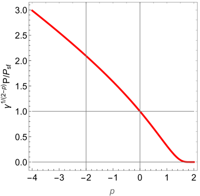
Figure 2: Enhancement of the power spectrum of curvature perturbations predicted by eq. (35).

The calculations for the single-field case presented in this Section can be easily generalized to a multi-field system. In Appendix B, we present an appropriate derivation, followed in Appendix C by a prescription for matching the perturbations in the sub- and super-Hubble regime.

V Numerical examples

In Section III, we have put forth a number a hypotheses. We argued that slow-roll fast-turn two-field inflationary models can be effectively described by a single-field theory with a time and $k$-dependent sound speed. We also proposed which combination of modes serves as an effective degree of freedom in the single-field theory. In this Section, we would like to corroborate those findings by presenting results of numerical calculations.

We study the evolution of the perturbations in the model described by the Lagrangian:

$$\mathcal{L}=\frac{e^{-2\phi_{2}/M}}{2}(\partial\phi_{1})^{2}-V_{\mathrm{inf}}(\phi_{1})+\frac{1}{2}(\partial\phi_{2})^{2}-\frac{1}{2}m_{2}^{2}\phi_{1}^{2}\,.$$ (39)

In this model, the interactions stemming from the non-canonical kinetic term can compensate the potential force acting on the field $\phi_{2}$. As a consequence, there may exist an inflationary trajectory, for which $\phi_{1}$ rolls slowly and $\phi_{2}$ stays constant. Models of this type have been analyzed by many authors and it was found that for certain values of the parameters one can describe the curvature perturbations with a single-field effective theory, either one with an effective sound speed smaller than one or one with modified dispersion relations.

Here we consider the approximation of quasi-de Sitter space, i.e., following Cremonini:2010ua ; Cremonini:2010sv , we assume that the Hubble parameter is practically constant and that the field $\phi_{1}$ moves negligibly during inflation, so all the quantities defined in terms of the homogeneous background are also practically constant. In this approximation, equations of motion resulting from (39) assume the form (B.58) with (B.60) and (B.61), where $\eta_{\perp}=\frac{\dot{\phi}_{1}}{MH}$ can be much larger than 1. This approximation allows us to capture characteristic features of the evolution of the effective sound speed in various models with high accuracy (which is particularly important for $|\eta_{\perp}|\gg 1$), disentangling the effects of the changes in the sound speed from other time dependencies, e.g. those originating from time-dependent background. Of course, the MESS approach is completely general and does not require the simplifications discussed here, but our goal is to discuss it in the context of multi-field examples already worked out in the literature.

For numerical calculations, we use initial conditions (C.68) and (C.70) with $\theta_{0}=0$, integrating the equations of motion (B.58) with (B.60) and (B.61) twice: to cover both intitial conditions. In order to isolate the adiabatic mode that dominates after Hubble radius crossing, we preform the following unitary transformations of the two results corresponding to initial conditions. If the first initial condition leads to $u_{\sigma}^{(1)}=z_{1}$ and the second initial condition leads to $u_{\sigma}^{(2)}=z_{2}$, we consider combinations of the two solutions, corresponding to rotated vectors in (C.68):

$$\left(\begin{array}[]{c}\tilde{u}_{\sigma}^{(1)}\\ \tilde{u}_{\sigma}^{(2)}\end{array}\right)=\frac{1}{\sqrt{|z_{1}|^{2}+|z_{2}|^{2}}}\left(\begin{array}[]{cc}z_{1}^{\ast}&z_{2}^{\ast}\\ -z_{2}&z_{1}\end{array}\right)\left(\begin{array}[]{c}u_{\sigma}^{(1)}\\ u_{\sigma}^{(2)}\end{array}\right)\,.$$ (40)

At the end of numerical evolution, we have $\tilde{u}_{\sigma}^{(2)}\to 0$, and therefore we identify the freezing mode with $\tilde{u}_{\sigma}^{(1)}$ and the decaying mode with $\tilde{u}_{\sigma}^{(2)}$. According to our discussion in Appendix B, with freeze-in at sub-Hubble scales the freezing mode should correspond to $z_{2}=-\mathrm{i}z_{1}$ and we confirm this in our numerical examples.

We represent perturbations as instantaneous power spectra and normalize them to the corresponding instantaneous power spectra of curvature perturtbations in single-field models, as described in detail in Lalak:2007vi . We use color coding for different components and different initial conditions described in Table 1.

multi-field model
perturbation	mode (defined by the behavior of the adiabatic mode)	color coding
curvature	freezing	thick, black, solid
curvature	decaying	thin, black, dashed
entropy	freezing	thin, red, dashed
entropy	decaying	thin, red, solid
single-field effective model
curvature	$\tilde{v}_{k}$ given by eq. (6) evaluated for the solution of the equations of motion corresponding to the freezing adiabatic mode	thick, green, dashed
curvature	$\tilde{v}_{k}$ given by eq. (6) evaluated for the solution of the equations of motion corresponding to the decaying adiabatic mode	thick, yellow, dashed (only Fig. 6)

Table 1: Color coding of the perturbations in Figures 3-6

.

V.1 Single-field effective theories with reduced sound speed

For the first numerical example, we assume $\eta_{\perp}=30$ and $\nu=10^{2}$, which leads to the effective sound speed $\tilde{v}_{k}^{2}=0.0265\approx 1/37.7$. Evolution of the effective sound speed calculated from (6) and evolution of adiabatic perturbations is shown in Figure 3. We find exquisite consistency at all scales between the predictions of the full two-field model and the effective single-field theory with a MESS sound speed.

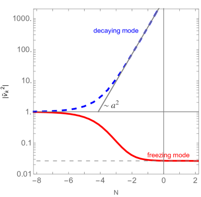
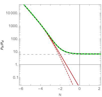
Figure 3: Numerical calculations in single-field effective theories with constant reduced sound speed; model described in Section V.1. Left panel: evolution of the sound speed given by eq. (6) for initial conditions leading to a freezing adiabatic mode (red solid line) and for initial conditions leading to a decaying adiabatic mode (blue dashed lines); thin dashed line corresponds to the value (22). Right panel: evolution of the instantaneous power spectra in the full theory and in the effective theory; color coding described in Table 1; thin dashed line corresponds to the asymptotic value (36). $N=0$ corresponds to the Hubble radius crossing

V.2 Single-field effective theories with modified dispersion relations

For the second numerical example, we assume $\eta_{\perp}=300$ and $\nu=10$. This model is not described by an effective single-field theory with a constant, reduced sound speed, but rather by by an effective single-field theory with modified dispersion relations. Evolution of the effective sound speed calculated from (6) and evolution of adiabatic perturbations is shown in Figure 4. We again find exquisite consistency at all scales between the predictions of the full two-field model and the effective single-field theory with a MESS sound speed.

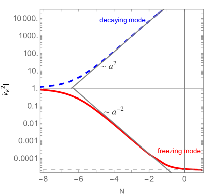
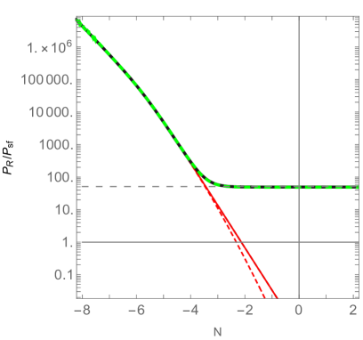
Figure 4: Numerical calculations in single-field effective theories with modified dispersion relations; model described in Section V.2. Left panel: evolution of the sound speed given by eq. (6) for initial conditions leading to a freezing adiabatic mode (red solid line) and for initial conditions leading to a decaying adiabatic mode (blue dashed lines); of thin dashed lines, one corresponds to the value (22) and the other shows that the sound speed decreases as $\sim a^{-2}$. Right panel: evolution of the instantaneous power spectra in the full theory and in the effective theory; color coding described in Table 1; thin dashed line corresponds to the asymptotic value (37). $N=0$ corresponds to the Hubble radius crossing

V.3 Hyperinflation

If the Lagrangian mass term for the entropy perturbations is small compared to other scales, the mass of these perturbations is dominated by the ‘geometrical’ $-2H^{2}\eta_{\perp}^{2}$ term, which in our example is related to the negative curvature of the field space. Such a negative mass term leads to instability and to a very strong enhancement of the amplitude of the perturbations. This phenomenon was first described in Cremonini:2010ua , which dubbed it transient tachyonic instability around the Hubble radius, and after a decade it was rediscovered in Brown:2017osf , which called it hyperinflation, and further analyzed in Mizuno:2017idt . In a slightly different context, sidetracked inflation models with a negative effective sound speed were discussed in Garcia-Saenz:2018ifx ; Fumagalli:2019noh . In all works mentioned above, inflation was realized on a steep potential in a hyperbolic field space.

It is interesting to note that hyperinflation can also be described in our effective single-field approach, albeit with a sound speed $\tilde{v}_{k}^{2}$ which changes sign during evolution. We demonstrate this numerically by an example with $\eta_{\perp}=300$ and $\nu=-10^{4}$. Evolution of the effective sound speed calculated from (6) and evolution of adiabatic perturbations is shown in Figure 5. We find exquisite consistency at all scales between the predictions of the full two-field model and the effective single-field theory with a MESS sound speed.

In Cremonini:2010ua , hyperinflation was described as an intrinsically two-field phenomenon. However, Brown:2017osf hinted at a curious property, determined numerically, that the freezing adiabatic mode is obtained from a single, well-defined initial mode. Here we confirm this observation and show that the evolution of that mode can be understood in effective theory with a time-dependent sound speed that starts at a canonical value of 1 and then goes imaginary.

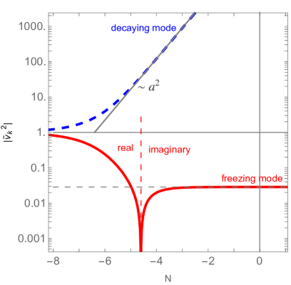
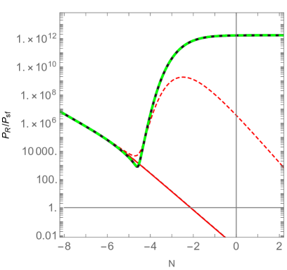
Figure 5: Numerical calculations in single-field effective theories for hyperinflation; model described in Section V.3. Left panel: evolution of the sound speed given by eq. (6) for initial conditions leading to a freezing adiabatic mode (red solid line) and for initial conditions leading to a decaying adiabatic mode (blue dashed lines); change of sign of the sound speed squared, i.e. transition from real to imaginary sound speed, is indicated; thin dashed line corresponds to the value (22). Right panel: evolution of the instantaneous power spectra in the full theory and in the effective theory; color coding described in Table 1; $N=0$ corresponds to the Hubble radius crossing

V.4 Single-field description for models with light entropy modes that cannot be integrated out

In Section III, we showed how the MESS approach allows to formulate a single-field description for models which were previously studied in the literature by integrating out entropy modes. Here we will consider the case in which the approach based on integrating out entropy modes cannot be applied, i.e. the first two terms in eq.(13) cannot be neglected, and no simple algebraic relation between $\zeta$ and $Q_{\sigma}$ holds at all times. In these cases the MESS approach can still be used to compute the effective sound speed of each independent quantum degree of freedom of the system. While from a field theoretic point of view the fact that there are two light degrees of freedom would be interpreted as the non existence of a single-field description, the effective sound of the appropriately rotated modes allows to compute the final value of the full curvature spectrum by studying the evolution of a single degree of freedom, providing a single-field description.

We consider a model with light entropy perturbations, $\nu=0$ and moderate kinetic coupling between perturbations, $\eta_{\perp}=0.3$. Such models were proposed in Cremonini:2010sv to explain in an alternative way the red tilt of the power spectrum of adiabatic perturbations; later they were rediscovered and analyzed anew in an improved way, invoking symmetries of the theory Achucarro:2016fby . Our particular model has entropy perturbations slowly decaying, so the sourcing of the adiabatic perturbations eventually becomes ineffective; had we chosen $\nu=-2\eta_{\perp}^{2}$, the amplitude of entropy perturbations would remain nearly constant and the sourcing could last much longer.

In these models, adiabatic perturbations are sourced by entropy perturbations on super-Hubble scales, which corresponds to the situation described in Section III.2.2, with the sound speed diverging to infinity. A closer inspection shows Cremonini:2010sv that the amplitude of the adiabatic perturbations grows as $\sim\eta_{\perp}N$ on super-Hubble scales, hence the sound speed increases as $\sim a^{2-\eta_{\perp}}$, according to eq. (18). Similarly, the sound speed for of the decaying mode increases as $a^{2+\eta_{\perp}}$. This is consistent with our findigs in Section II.2 that $\tilde{v}_{k}\sim a^{2}$ marks a divide between freezing and decaying solutions.

In Figure 6, we show that, similarly to the case of hyperinflation, the sound speed $\tilde{v}_{k}^{2}$ changes sign during evolution. We also show the evolution of adiabatic and entropy perturbations.

The evolution of the freezing and decaying modes of the adiabatic perturbations is compared to the evolution of a single-field effective description with an effective sound speed given by (6) with an appropriate set of initial conditions. We find a good agreement betwen the predictions of the full theory and two single-field effective theories with different effective sound speeds. Depending on the phase of the evolution, either the freezing or the decaying mode dominates the instantaneous power spectrum and the late-time domination of the freezing mode starts only after Hubble radius crossing. This shows that the model cannot be approximated by an effective single-field theory at all times – we need to combine two single-field theories with two effective, independent sound speeds to obtain correct predictions for the curvature perturbations at all times, but the freezing mode is sufficient to compute the final value. Our numerical analyses also point to the fact that this conclusion holds true for all models described in Section III.2.2, i.e. models with sourcing of the adiabatic perturbations on super-Hubble scales.

Since those models can be studied also by integrating out entropy modes, the fact that a single EFT valid at any time does not exist, would also be a limitation of the EFT obtained using that method, and is an intrinsic property of these systems, independent of the method adopted to study them.

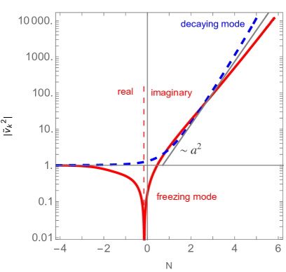
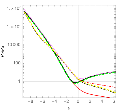
Figure 6: Numerical calculations in single-field effective theories for light entropy perturbations; model described in Section V.4. Left panel: evolution of the sound speed given by eq. (6) for initial conditions leading to a freezing adiabatic mode (red solid line) and for initial conditions leading to a decaying adiabatic mode (blue dashed lines); change of sign of the sound speed squared, i.e. transition from real to imaginary sound speed, is indicated; thin dashed line corresponds to the value (22). Right panel: evolution of the instantaneous power spectra in the full theory and in the effective theory; color coding described in Table 1; $N=0$ corresponds to the Hubble radius crossing; the pink line corresponds to the total curvature power spectrum.

VI Discussion

In the context of cosmological perturbations, the existence of a single-field effective theory requires that the degree of freedom corresponding to the freezing mode, accounting for the entire amplitude of adiabatic perturbations at the end of inflation, evolves independently of all other perturbations. Those perturbations can be dynamical, but as their masses are larger than the Hubble parameter, their amplitudes decrease as power law functions of the scale factor. Hence the notion of the effective theory in cosmology is different from the one used in particle physics, where decoupling normally means that other degrees of freedom are too heavy to be excited.

At face value, our effective description of single-field inflation resembles the quadratic part of the action for adiabatic perturbations derived in Cheung:2007st . However, we would like to point out that the sound speed in that reference is a function of time only. Using a very simple model with a large and constant turning rate, analyzed previously in Cremonini:2010ua ; Baumann:2011su , we have shown that the evolution of the adiabatic perturbations is correctly accounted for by a sound speed that is both time- and momentum-dependent. Hence our approach generalizes the effective theory of inflation of Cheung:2007st in a non-trivial way, including the effects of entropy.

A truly effective single-field theory has only one relevant degree of freedom that fully accounts for both the power spectrum of the adiabatic perturbations and for higher-order correlation functions of adiabatic perturbations. Although such a mode has both the adiabatic and the entropic components, a known effective sound speed (6) provides an algebraic relation between these two components, so the entropic component is no longer an independent quantity. Such an effective description requires just one effective sound speed, because other degrees of freedom are assumed to have decayed before the Hubble radius crossing and thus do not contribute to correlation functions of adiabatic perturbations. In this sense, the models analyzed in Sections V.1-V.3 have a single-field effective theory, while the model described in Section V.4 does not. In this latter case, there is a non-negligible independent degree of freedom that significantly contributes to the amplitude of adiabatic perturbations around the Hubble crossing. We can therefore conclude that a momentum-dependent effective sound speed parametrizes single-field effective theories of inflation and provides an effective description of the adiabatic perturbations when such a theory cannot be formulated.

There is also an alternative, more general view of the models discussed in Section V, which, however, involves more input and is thus less predictive. Since the perturbed energy-stress tensor enters Einstein equations and does not rely on a particular model of multi-field inflation, the evolution of the adiabatic component of each degree of freedom is described by eq. (7) with an appropriate sound speed. We can define a number of different effective sound speeds to account for the evolution of all degrees of freedom, as we have done in Section V.4. This approach allows us to describe also the evolution of adiabatic perturbations (without resorting explicitly to the notion of entropy perturbations) in models which do not admit an effective single-field theory.

The effective field theory of inflation Cheung:2007st is based on the assumption that only one scalar degree of freedom is present, and is formulated in the uniform field gauge, also called unitary gauge, in which an action invariant under time-dependent space diffeomerphism can be written without any matter perturbation terms. The unitary gauge does not coincide with the comoving slices gauge in multi-field systems Romano:2018frb , so in general the effective theory of inflation cannot be applied to multi-field systems in which there is no gauge in which the matter perturbations can be completely set to zero (in other words, entropy perturbations) cannot be neglected. Nevertheless, there can also be effective entropy in the comoving slicea gauge in modified gravity theories with a single scalar degree of freedom, e.g. in such as KGB models Vallejo-Pena:2019hgv , which can be described by the effective theory of inflation. These modified gravity theories give rise to a modification of the dispersion relation, related to extrinsic curvature terms of the effective action Cheung:2007st ; Baumann:2011su and leading to a momentum-effective sound speed, consistent with the MESS approach, once the gauge transformation from the unitary to the comoving slices gauge is performed Vallejo-Pena:2019hgv . In contrast, effective theory of inflation cannot be applied to multi-fields systems where there is no gauge in which the action can only be written in term of geometrical quantitites This is confirmed, e.g. by the modified dispersion relation obtained in eq. (B.6) in Baumann:2011su , which has a different momentum dependency from the one which arises from extrinsic curvature terms in the effective theory of inflation, as shown in eq. (3.22) in Baumann:2011su , associated to intrinsic entropy in single field modified gravity theories.

In summary, the advantages of the MESS are that it relates the effective sound speed to the energy-stress tensor in a model-independent way. It also does not require integrating out e ntropy modes and it is not based on any further approximation, such as the decoupling limit often assumed in the effective theory of inflation. Thus it gives a general model-independent description of adiabatic perturbations, valid at any energy scale. It also makes explicit the relation between the entropy of the mulfi-field theory and the momentum dependent effective sound speed of the corresponding single field effective theory, and that it can be computed directly from the solutions of the matter perturbations equations without the need of computing an effective action.

The definition of MESS is completely general, and can be applied to any multifields model, including models with sharp turns of the classical field trajectory. It can also be applied to modified gravity theories Vallejo-Pena:2019hgv , and more complex systems involving gauge fields, such as axion inflation, as long as the comoving gauge of the total effective energy-momentum tensor is properly computed. The ungauged tensor can always be computed analytically, while the comoving gauge condition can be added to the field equations to be solved numerically, in case it cannot be used to simply them analytically.

As long as numerical calculations can be carried out with sufficient accuracy, the method can be applied without any restrictions to any multi-field model, with no restriction on the classical field trajectory. The computation of the MESS involves in some cases the cancellation between very small numbers, which requires the use of a sufficiently high numerical accuracy to avoid instabilities, but for models where entropy modes cannot be integrated out, this is the only approach which can be adopted to obtain a single-field description capable of predicting the time dependence of the adiabatic perturbations of the full multi-field theory.

VII Conclusions

In this work, we presented a formulation of a single-field effective description of inflation, making use of a recently advocated approach based on the momentum-dependent effective sound speed (MESS) Romano:2018frb . We have shown that this formulation includes a number of multi-field models that were considered in the literature in the last decade. We have identified the effective degree of freedom and shown how its evolution can be treated independently of other degrees of freedom, even at scales at which the amplitudes the latter are not suppressed yet. We have also applied the MESS approach to a models with light entropy perturbations, which does not admit an effective field theory obtained by integrating out entropy modes. Hence we have demonstrated that the MESS approach, which generalizes the notion of single-field effective theory of inflation, is a powerful and useful scheme for studying a wide range of inflationary models.

Appendix A MESS of multiple scalar fields

The energy-stress tensor for the system described by the action given in eq.(12) is

$$T^{\mu}{}_{\nu}=G_{IJ}\left(\Phi^{K}\right)\partial^{\mu}\Phi^{I}\partial_{\nu}\Phi^{J}+\delta^{\mu}{}_{\nu}\left[-\frac{1}{2}G_{IJ}\left(\Phi^{K}\right)\partial_{\lambda}\Phi^{I}\partial^{\lambda}\Phi^{J}-V\left(\Phi^{K}\right)\right]\,.$$ (A.41)

The scalar fields at linear order can be expanded as $\Phi^{K}(x^{\mu})=\phi^{K}(t)+\delta\phi^{K}(x^{\mu})$, where the background parts of the scalar fields satisfy the following equations of motion

$$\ddot{\phi}^{I}+3H\dot{\phi}^{I}+\Gamma^{I}_{JK}\dot{\phi}^{J}\dot{\phi}^{K}+G^{IJ}\left(\phi^{K}\right)V_{,J}\left(\phi^{J}\right)=0\,,$$ (A.42)

where $\Gamma^{I}_{JK}$ are the Christoffel symbols corresponding to the fields space metric $G_{IJ}\left(\phi^{K}\right)$, and we denote the partial derivative respect to the field $\phi^{J}$ according to $V_{,J}\left(\phi^{J}\right)=\frac{\partial}{\partial\phi^{J}}V\left(\phi^{J}\right)$. The background energy density and pressure are

$$\rho =\frac{1}{2}\dot{\sigma}^{2}+V\left(\phi^{K}\right)\,,$$ (A.43)

$$P =\frac{1}{2}\dot{\sigma}^{2}-V\left(\phi^{K}\right)\,,$$ (A.44)

where $\dot{\sigma}^{2}=G_{IJ}\left(\phi^{K}\right)\dot{\phi}^{I}\dot{\phi}^{J}$. The components of the perturbed energy-stress tensor of the two scalar fields system, without gauge fixing, are

$$\delta T^{0}{}_{0} =-\frac{1}{2}G_{IJ}\left(\phi^{K}\right)\left(\dot{\phi}^{I}\dot{\delta\phi}^{J}+\dot{\phi}^{J}\dot{\delta\phi}^{I}\right)+\dot{\sigma}^{2}A-\delta\phi^{k}\left(\frac{1}{2}\dot{\phi}^{I}\dot{\phi}^{J}G_{IJ},_{K}\left(\phi^{K}\right)+V_{,K}\left(\phi^{K}\right)\right)\,,$$

$$\delta T^{i}{}_{j} =\delta^{i}_{j}\left[\frac{1}{2}G_{IJ}\left(\phi^{K}\right)\left(\dot{\phi}^{I}\dot{\delta\phi}^{J}+\dot{\phi}^{J}\dot{\delta\phi}^{I}\right)-\dot{\sigma}^{2}A+\delta\phi^{k}\left(\frac{1}{2}\dot{\phi}^{I}\dot{\phi}^{J}G_{IJ},_{K}\left(\phi^{K}\right)-V_{,K}\left(\phi^{K}\right)\right)\right]\,,$$

$$\delta T^{0}{}_{i} =-\partial_{i}\left[\frac{G_{IJ}\left(\phi^{K}\right)\dot{\phi}^{I}\delta\phi^{J}}{a}\right]\,.$$ (A.45)

Under an infinitesimal time translation $t\to t+\delta t$ the fields perturbations transform according to the gauge transformation

$$\widetilde{\delta\phi}^{K} =\delta\phi^{K}-\dot{\phi}^{K}\delta t\,.$$ (A.46)

From these equations we can find the time translation $\delta t_{c}$ necessary to go to the comoving gauge, by imposing the comoving gauge condition $(\delta T^{0}{}_{i})_{c}=0\rightarrow G_{IJ}\left(\phi^{K}\right)\dot{\phi}^{I}\widetilde{\delta\phi}^{J}=0$, obtaining

$$\delta t_{c} =\frac{G_{IJ}\left(\phi^{K}\right)\dot{\phi}^{I}\delta\phi^{J}}{\dot{\sigma}^{2}}\,.$$ (A.47)

We can now compute the gauge invariant comoving field perturbations according to

$$U^{K}=\delta\phi^{K}-\dot{\phi}^{K}\delta t_{c}=\delta\phi^{K}-\dot{\phi}^{K}\frac{G_{IJ}\left(\phi^{K}\right)\dot{\phi}^{I}\delta\phi^{J}}{\dot{\sigma}^{2}}\,,$$ (A.48)

and the comoving pressure and energy density perturbations

$$\alpha =\delta P_{c}=\frac{1}{2}G_{IJ}\left(\phi^{K}\right)\left(\dot{\phi}^{I}\dot{U}^{J}+\dot{\phi}^{J}\dot{U}^{I}\right)-\dot{\sigma}^{2}\gamma+U^{k}\left(\frac{1}{2}\dot{\phi}^{I}\dot{\phi}^{J}G_{IJ},_{K}\left(\phi^{K}\right)-V_{,K}\left(\phi^{K}\right)\right)\,,$$ (A.49)

$$\beta =\delta\rho_{c}=\frac{1}{2}G_{IJ}\left(\phi^{K}\right)\left(\dot{\phi}^{I}\dot{U}^{J}+\dot{\phi}^{J}\dot{U}^{I}\right)-\dot{\sigma}^{2}\gamma+U^{k}\left(\frac{1}{2}\dot{\phi}^{I}\dot{\phi}^{J}G_{IJ},_{K}\left(\phi^{K}\right)+V_{,K}\left(\phi^{K}\right)\right)\,.$$ (A.50)

After replacing eq.(A.48) and eq.(A.42) into these expressions we find

$$U^{k}V_{,K}\left(\phi^{K}\right) =\frac{1}{2}G_{IJ}\left(\phi^{K}\right)\left(\dot{\phi}^{I}\dot{U}^{J}+\dot{\phi}^{J}\dot{U}^{I}\right)+U^{k}\frac{1}{2}\dot{\phi}^{I}\dot{\phi}^{J}G_{IJ},_{K}\left(\phi^{K}\right)=-\dot{\sigma}^{2}\frac{\Theta}{4}\,,$$ (A.51)

$$\alpha =-\dot{\sigma}^{2}\gamma=-\dot{\sigma}^{2}\frac{\dot{\zeta}}{H}\,,$$ (A.52)

$$\beta =-\dot{\sigma}^{2}\left(\gamma+\frac{\Theta}{2}\right)=-\dot{\sigma}^{2}\left(\frac{\dot{\zeta}}{H}+\frac{\Theta}{2}\right)\,,$$ (A.53)

where we have used the perturbed Einstein’s equation $\gamma=\dot{\zeta}/H$, and we have defined the function $\Theta$ according to

$$\Theta \equiv-\frac{4\dot{\phi}_{1}\dot{\phi}_{2}}{\dot{\sigma}^{3}}\sqrt{G}\left(\frac{\delta\phi_{1}}{\dot{\phi}_{1}}-\frac{\delta\phi_{2}}{\dot{\phi}_{2}}\right)V_{,s}=\frac{4}{\dot{\sigma}^{2}}Q_{,s}V_{,s}\,,$$ (A.54)

where $G$ is the determinant of the fields space metric $G_{IJ}\left(\phi^{K}\right)$, i.e. $G\equiv\det{(G_{IJ})}$, $Q_{,s}\equiv Q_{,K}e^{K}_{s}$ $V_{,s}\equiv V_{,K}e^{K}_{s}$, and

$$e^{K}_{s} =\left(e^{1}_{s},e^{2}_{s}\right)=\left(\frac{G_{21}\dot{\phi}_{1}+G_{22}\dot{\phi}_{2}}{\dot{\sigma}\sqrt{G}},-\frac{G_{11}\dot{\phi}_{1}+G_{12}\dot{\phi}_{2}}{\dot{\sigma}\sqrt{G}}\right)\,.$$ (A.55)

Finally the MESS is given by

$$\tilde{v}_{k}^{2}(t) =\left(1+\frac{H\Theta}{2\dot{\zeta}}\right)^{-1}=\left(1+\frac{2HV_{,s}Q_{,s}}{\dot{\zeta}\dot{\sigma}^{2}}\right)^{-1}=\left(1-\frac{2H^{2}\eta_{\perp}Q_{,s}}{\dot{\zeta}\dot{\sigma}}\right)^{-1}\,,$$ (A.56)

where

$$\eta_{\perp}\equiv-\frac{V_{,s}}{H\dot{\sigma}}\,.$$ (A.57)

Appendix B Multi-field case

The calculation given in Section IV can be easily generalized to a system of $N$ coupled linear and homogeneous equations, which can be written as:

$$\frac{\mathrm{d}^{2}\vec{\mathcal{U}}}{\mathrm{d}\eta^{2}}+\mathbb{L}(\eta)\frac{\mathrm{d}\vec{\mathcal{U}}}{\mathrm{d}\eta}+\mathbb{M}(\eta)\vec{\mathcal{U}}=0\,,$$ (B.58)

where $\vec{\mathcal{U}}=(\mathcal{U}_{1}(\eta),\ldots,\mathcal{U}_{N}(\eta))$ and $\mathbb{L}(\eta)$, $\mathbb{M}(\eta)$ are real-valued $N\times N$ matrices, which are functions of the independent variable $\eta$. It is easy to show that for $\mathbb{L}=0$ and $\mathbb{M}^{T}=\mathbb{M}$ the Wronskian defined as:

$$W(\eta)\equiv\vec{\mathcal{U}}^{\dagger}\frac{\vec{\mathcal{U}}}{\mathrm{d}\eta}-\left(\frac{\mathrm{d}\vec{\mathcal{U}}}{\mathrm{d}\eta}\right)^{\dagger}\vec{\mathcal{U}}$$ (B.59)

does not depend on $\eta$.

The equations of motion for the two-field system of adiabatic and entropy perturbations (13)-(14) can be transformed so that we can make use of this fact. We first redefine perturbations as $\vec{u}=(aQ_{\sigma},aQ_{s})$ and identify $\eta$ with conformal time. We obtain a system of equations of the form (B.58) with:

$$\mathbb{L}=\left(\begin{array}[]{cc}0&\frac{2\eta_{\perp}}{\eta}\\ -\frac{2\eta_{\perp}}{\eta}&0\end{array}\right)$$ (B.60)

and

$$\mathbb{M}=\left(k^{2}-\frac{2}{\eta^{2}}\right)\,\mathbf{1}+\left(\begin{array}[]{cc}0&-\frac{4\eta_{\perp}}{\eta^{2}}\\ -\frac{2\eta_{\perp}}{\eta^{2}}&\frac{\nu}{\eta^{2}}\end{array}\right)\,,$$ (B.61)

where $\nu=\frac{m_{s}^{2}}{H^{2}}-2\eta_{\perp}^{2}$ and we used de Sitter approximation again . We then define

$$\vec{\mathcal{U}}=\mathbb{R}\vec{u}$$ (B.62)

with

$$\mathbb{R}(\eta)=\left(\begin{array}[]{cc}\cos\left(\eta_{\perp}\log\left(\frac{\eta}{\eta_{0}}\right)\right)&\sin\left(\eta_{\perp}\log\left(\frac{\eta}{\eta_{0}}\right)\right)\\ -\sin\left(\eta_{\perp}\log\left(\frac{\eta}{\eta_{0}}\right)\right)&\cos\left(\eta_{\perp}\log\left(\frac{\eta}{\eta_{0}}\right)\right)\end{array}\right)\,,$$ (B.63)

where $\eta_{0}$ is an arbitrary constant. In terms of the new variable $\vec{\mathcal{U}}$, the equation of motion (B.58) reads:

$$\frac{\mathrm{d}^{2}\vec{\mathcal{U}}}{\mathrm{d}\eta^{2}}+\left[\left(k^{2}+\frac{\eta_{\perp}^{2}-2}{\eta^{2}}\right)\mathbf{1}+\frac{1}{\eta^{2}}\mathbb{R}\mathcal{M}\mathbb{R}^{T}\right]\vec{\mathcal{U}}=0\,,$$ (B.64)

where

$$\mathcal{M}=\left(\begin{array}[]{cc}0&-3\eta_{\perp}\\ -3\eta_{\perp}&\nu\end{array}\right)\,,$$ (B.65)

The conserved Wronskian (B.59) reads:

$$W(\eta)=\vec{u}^{\dagger}\frac{\mathrm{d}\vec{u}}{\mathrm{d}\eta}-\left(\frac{\mathrm{d}\vec{u}}{\mathrm{d}\eta}\right)^{\dagger}\vec{u}+\frac{2\eta_{\perp}}{\eta}\vec{u}^{\dagger}\mathbb{E}\vec{u}\,,$$ (B.66)

where we denoted:

$$\mathbb{E}=\left(\begin{array}[]{cc}0&1\\ -1&0\end{array}\right)$$ (B.67)

and made use of the fact that $\frac{\mathrm{d}\mathbb{R}}{\mathrm{d}\eta}=\frac{\eta_{\perp}}{\eta}\mathbb{R}\mathbb{E}$.

This form of the Liouville equation can be used to identify the initial Bunch-Davis conditions in a coupled multi-field system and to match those initial condition with the late-time behavior of the perturbations. We comment on these issues below.

Appendix C Matching curvature and entropy perturbations in the sub- and super-Hubble regime

Based on the results of Appendix B, we can comment on the choice of the Bunch-Davies vacuum as an initial state for the adiabatic and entropy perturbations and on a simple way in which that initial state can be matched with the asymptotic late-times solutions of the equations of motion. Deep inside the Hubble radius, i.e. for $\eta\to-\infty$, eq. (B.64) becomes an equation of motion for a harmonic oscillator and it has two independent positive-frequency solutions:

$$\vec{\mathcal{U}}^{(1)}(\eta)\sim\frac{e^{-\mathrm{i}k\eta}}{\sqrt{2k}}\vec{\mathcal{U}}^{(1)}_{0}\qquad\textrm{and}\qquad\vec{\mathcal{U}}^{(2)}(\eta)\sim\frac{e^{-\mathrm{i}k\eta}}{\sqrt{2k}}\vec{\mathcal{U}}^{(2)}_{0}\,,$$ (C.68)

where $\vec{\mathcal{U}}^{(1)}_{0}$ and $\vec{\mathcal{U}}^{(2)}_{0}$ are constant vectors satisfying

$$\vec{\mathcal{U}}^{(I)\dagger}_{0}\vec{\mathcal{U}}^{(J)}_{0}=\delta_{IJ}\,.$$ (C.69)

These vectors can be parametrized as:

$$\vec{\mathcal{U}}^{(1)}_{0}=\left(\begin{array}[]{c}\cos\theta_{0}\\ \sin\theta_{0}e^{i\phi_{0}}\end{array}\right)\qquad\textrm{and}\qquad\vec{\mathcal{U}}^{(2)}_{0}=\left(\begin{array}[]{c}-\sin\theta_{0}e^{-i\phi_{0}}\\ \cos\theta_{0}\end{array}\right)\,.$$ (C.70)

In terms of perturbations $\vec{u}$, the solution (C.68) reads:

$$\vec{u}^{(1)}\sim\frac{e^{-\mathrm{i}k\eta}}{\sqrt{2k}}\left(\begin{array}[]{c}\cos\theta_{0}\cos\left(\eta_{\perp}\log\left(\frac{\eta}{\eta_{0}}\right)\right)-e^{i\phi_{0}}\sin\theta_{0}\sin\left(\eta_{\perp}\log\left(\frac{\eta}{\eta_{0}}\right)\right)\\ \cos\theta_{0}\sin\left(\eta_{\perp}\log\left(\frac{\eta}{\eta_{0}}\right)\right)+e^{i\phi_{0}}\sin\theta_{0}\cos\left(\eta_{\perp}\log\left(\frac{\eta}{\eta_{0}}\right)\right)\end{array}\right)$$ (C.71)

and

$$\vec{u}^{(2)}\sim\frac{e^{-\mathrm{i}k\eta}}{\sqrt{2k}}\left(\begin{array}[]{c}-e^{-\mathrm{i}\phi_{0}}\sin\theta_{0}\cos\left(\eta_{\perp}\log\left(\frac{\eta}{\eta_{0}}\right)\right)-\cos\theta_{0}\sin\left(\eta_{\perp}\log\left(\frac{\eta}{\eta_{0}}\right)\right)\\ -e^{-\mathrm{i}\phi_{0}}\sin\theta_{0}\sin\left(\eta_{\perp}\log\left(\frac{\eta}{\eta_{0}}\right)\right)+\cos\theta_{0}\cos\left(\eta_{\perp}\log\left(\frac{\eta}{\eta_{0}}\right)\right)\end{array}\right)\,.$$ (C.72)

The modulus squared of the upper (adiabatic) component in (C.71) reads:

$$\left|u^{(1)}_{\sigma}\right|^{2}=\frac{1}{4k}\left(1+\cos 2\theta_{0}\cos\left(2\eta_{\perp}\log\left(\frac{\eta}{\eta_{0}}\right)\right)-\cos\phi_{0}\sin 2\theta_{0}\sin\left(2\eta_{\perp}\log\left(\frac{\eta}{\eta_{0}}\right)\right)\right)\,.$$ (C.73)

This expression is constant for $\theta_{0}=\pm\frac{\pi}{4}$ and $\phi_{0}=\frac{\pi}{2}$, which also corresponds to constant $|u^{(1)}_{s}|^{2}$, $|u^{(2)}_{\sigma}|^{2}$ and $|u^{(2)}_{s}|^{2}$. Our final results is, therefore:

$$\vec{u}^{(1)}\sim\frac{e^{-\mathrm{i}k\eta+\mathrm{i}\eta_{\perp}\log\left(\frac{\eta}{\eta_{0}}\right)}}{2\sqrt{k}}\left(\begin{array}[]{c}1\\ -\mathrm{i}\end{array}\right)\qquad\textrm{and}\qquad\vec{u}^{(2)}\sim\frac{e^{-\mathrm{i}k\eta-\mathrm{i}\eta_{\perp}\log\left(\frac{\eta}{\eta_{0}}\right)}}{2\sqrt{k}}\left(\begin{array}[]{c}-\mathrm{i}\\ 1\end{array}\right)\,.$$ (C.74)

Note that eq. (C.74) exhibits some redundancy, which was not visible in the intermediate steps leading to that result. A change in arbitrary constant $\eta_{0}$ can be extracted as an unphysical phase factor multiplying the solution.

The approximate solution (C.74) is reliable as long as the last term in eq. (B.64) is negligible. This is satified for $(k\eta)^{2}>\mathrm{max}\{\nu,3\eta_{\perp}\}$.

It is also interesting to study the late-time behavior of the system of equations (B.64) with (B.60) and (B.61), following the treatment in Cremonini:2010ua . In the limit $\eta\to 0^{-}$, we can neglect the $k$-dependent term and assume solutions of the form:

$$\vec{u}=\left(\frac{\eta}{\eta_{0}}\right)^{P}\left(\begin{array}[]{c}A_{\sigma}\\ A_{s}\end{array}\right)\,,$$ (C.75)

where $\eta_{0}$ represents the value of the conformal time at which the solution should be matched with the early-time solution. We obtain an algebraic equation:

$$\left(\begin{array}[]{cc}P(P-1)-2&2\eta_{\perp}(P-2)\\ -2\eta_{\perp}(P+1)&P(P-1)-2+\nu\end{array}\right)\left(\begin{array}[]{c}A_{\sigma}\\ A_{s}\end{array}\right)=0\,.$$ (C.76)

Eq. (C.76) has four nontrivial solutions for $p$:

$$P_{1} = -1\,,\qquad\textrm{with}\qquad\frac{A^{(1)}_{s}}{A^{(1)}_{\sigma}}=0$$ (C.77)

$$P_{2} = 2\,,\qquad\textrm{with}\qquad\frac{A^{(2)}_{s}}{A^{(2)}_{\sigma}}=\frac{6\eta_{\perp}}{\nu}$$ (C.78)

$$P_{3,4} = \frac{1}{2}\mp\mathrm{i}\sqrt{\nu+4\eta_{\perp}^{2}-\frac{9}{4}}\,,\qquad\textrm{with}\qquad\frac{A^{(3,4)}_{s}}{A^{(3,4)}_{\sigma}}=-\frac{\nu+4\eta_{\perp}^{2}}{\eta_{\perp}\left(3\pm 2\mathrm{i}\sqrt{\nu+4\eta_{\perp}^{2}-\frac{9}{4}}\right)}\,.$$ (C.79)

The last two solutions (C.79) correspond to the positive and negative frequency solutions for a massive mode, of mass squared $(\nu+4\eta_{\perp}^{2})H^{2}$. The first two solutions, eqs. (C.77)-(C.78) correspond to the growing and decaying part of a massless mode. It is also clear that the growing mode $\sim 1/\eta$ carries only the adiabatic component, i.e. in the considered model adiabatic perturbations can freeze in at some scale, while all entropy perturbations decay at late times.

The mode corresponding to the exponent $p_{4}$ corresponds to negative frequency. If the relative change of the sound speed is not much larger than one, this mode is not excited during the evolution of the perturbations. It is instructive to analyze the relations between the sub-Hubble solutions (C.74) and the solutions (C.77)-(C.79). This is particularly simple in the limit $\nu\to 0$, which will correspond to numerical examples to be discussed later. In this limit, we have:

$$A_{s}^{(1)}=0\,,\qquad A_{\sigma}^{(2)}\approx 0\,,\qquad A_{s}^{(3)}\approx\mathrm{i}A_{\sigma}^{(3)}\,.$$ (C.80)

Matching (C.74) with (C.77)-(C.79), we find that $\vec{u}^{(2)}$ corresponds to a massive mode with $p_{3}$, which decays on super-Hubble scales, while $\vec{u}^{(1)}$ is a combination of a growing mode corresponding to $p_{1}$ and the decaying massive mode corresponding to $p_{2}$, with $A_{\sigma}^{(1)}\approx-\mathrm{i}A_{s}^{(2)}$.

A general late-times solution of (B.58) can therefore be written as:

$$\vec{u}=\sum_{I=1}^{4}\left(\frac{\eta}{\eta_{0}}\right)^{P_{I}}\left(\begin{array}[]{c}A^{(I)}_{\sigma}\\ A^{(I)}_{s}\end{array}\right)\,,$$ (C.81)

where for a given $I$ the coefficients $A^{(I)}_{\sigma}$ and $A^{(I)}_{s}$ satisfy the relations in respective eqs. (C.77)-(C.79). Plugging (C.81) into the expression for the conserved Wronskian, we find:

$$W=-\frac{\mathrm{i}\left(\nu+4\eta_{\perp}^{2}\right)}{\eta_{\perp}\eta_{0}}\,\mathrm{Im}\left(A^{(1)}_{\sigma}A_{s}^{(2)\ast}\right)-\frac{\mathrm{i}\left(\nu+4\eta_{\perp}^{2}\right)\sqrt{\nu+4\eta_{\perp}^{2}-\frac{9}{4}}}{2\eta_{\perp}^{2}\eta_{0}}\left(\left|A^{(3)}_{\sigma}\right|^{2}-\left|A^{(4)}_{\sigma}\right|^{2}\right)\,.$$ (C.82)

In the limit $\nu\to 0$ considered above, this reduces to:

$$W=-\frac{4\mathrm{i}\eta_{\perp}}{\eta_{0}}|A^{(1)}_{\sigma}|^{2}\,.$$ (C.83)

As the Wronskian (C.83) is conserved and equal $-\mathrm{i}$, we find that $|A_{\sigma,1}|^{2}=\eta_{0}/4\eta_{\perp}$, which leads to the following prediction for the power spectrum of the adiabatic perturbations:

$$\frac{\mathcal{P}}{\mathcal{P}_{\mathrm{sf}}}=\frac{|k\eta_{0}|^{3}}{2\eta_{\perp}}\,.$$ (C.84)

Since $\eta_{0}$ corresponds to matching between the early- and late-time solutions, and we argued that for $\nu\to 0$ we have $\eta_{0}=-\sqrt{3\eta_{\perp}}/k$, we obtain:

$$\frac{\mathcal{P}}{\mathcal{P}_{\mathrm{sf}}}=\frac{3\sqrt{3}}{2}\eta_{\perp}^{1/2}\,.$$ (C.85)

We note that this equation has the same parametric form as eq. (37) and the numerical prefactor $\sim 2.6$ in eq. (C.85) is very close to that eq. (37). This is a remarkable consistency, given our crude approach to solving the equations of motion for the two-field system, relying on matching between the early- and late-time asymptotic solutions.

References

- (1) A. E. Romano and S. A. Vallejo-Peña, Phys. Lett. B784, 367 (2018), arXiv:1806.01941.
- (2) A. Achucarro, J.-O. Gong, S. Hardeman, G. A. Palma, and S. P. Patil, JCAP 01, 030 (2011), arXiv:1010.3693.
- (3) A. Achucarro, S. Hardeman, J. M. Oberreuter, K. Schalm, and T. van der Aalst, JCAP 03, 038 (2013), arXiv:1108.2278.
- (4) G. Shiu and J. Xu, Phys. Rev. D 84, 103509 (2011), arXiv:1108.0981.
- (5) A. Avgoustidis et al., JCAP 02, 038 (2012), arXiv:1110.4081.
- (6) A. Achucarro, J.-O. Gong, S. Hardeman, G. A. Palma, and S. P. Patil, JHEP 05, 066 (2012), arXiv:1201.6342.
- (7) S. Cespedes, V. Atal, and G. A. Palma, JCAP 05, 008 (2012), arXiv:1201.4848.
- (8) A. Avgoustidis et al., JCAP 06, 025 (2012), arXiv:1203.0016.
- (9) X. Chen and Y. Wang, JCAP 09, 021 (2012), arXiv:1205.0160.
- (10) S. Pi and M. Sasaki, JCAP 10, 051 (2012), arXiv:1205.0161.
- (11) X. Gao, D. Langlois, and S. Mizuno, JCAP 10, 040 (2012), arXiv:1205.5275.
- (12) A. Achucarro et al., Phys. Rev. D 86, 121301 (2012), arXiv:1205.0710.
- (13) H. Collins, R. Holman, and A. Ross, JHEP 02, 108 (2013), arXiv:1208.3255.
- (14) C. P. Burgess, M. W. Horbatsch, and S. P. Patil, JHEP 01, 133 (2013), arXiv:1209.5701.
- (15) R. Gwyn, G. A. Palma, M. Sakellariadou, and S. Sypsas, JCAP 04, 004 (2013), arXiv:1210.3020.
- (16) T. Noumi, M. Yamaguchi, and D. Yokoyama, JHEP 06, 051 (2013), arXiv:1211.1624.
- (17) E. Dimastrogiovanni, M. Fasiello, and A. J. Tolley, JCAP 02, 046 (2013), arXiv:1211.1396.
- (18) N. Bartolo, D. Cannone, and S. Matarrese, JCAP 10, 038 (2013), arXiv:1307.3483.
- (19) S. Garcia-Saenz and S. Renaux-Petel, JCAP 11, 005 (2018), arXiv:1805.12563.
- (20) A. Durakovic, P. Hunt, S. P. Patil, and S. Sarkar, SciPost Phys. 7, 049 (2019), arXiv:1904.00991.
- (21) L. Pinol, JCAP 04, 002 (2021), arXiv:2011.05930.
- (22) H. Kodama and M. Sasaki, Prog. Theor. Phys. Suppl. 78, 1 (1984).
- (23) C. Gordon, D. Wands, B. A. Bassett, and R. Maartens, Phys. Rev. D63, 023506 (2001), arXiv:astro-ph/0009131.
- (24) S. Groot Nibbelink and B. J. W. van Tent, Class. Quant. Grav. 19, 613 (2002), arXiv:hep-ph/0107272.
- (25) A. J. Tolley and M. Wyman, Phys. Rev. D 81, 043502 (2010), arXiv:0910.1853.
- (26) S. Cremonini, Z. Lalak, and K. Turzynski, JCAP 03, 016 (2011), arXiv:1010.3021.
- (27) D. Baumann and D. Green, JCAP 09, 014 (2011), arXiv:1102.5343.
- (28) S. Garcia-Saenz, S. Renaux-Petel, and J. Ronayne, JCAP 07, 057 (2018), arXiv:1804.11279.
- (29) J. Fumagalli, S. Garcia-Saenz, L. Pinol, S. Renaux-Petel, and J. Ronayne, Phys. Rev. Lett. 123, 201302 (2019), arXiv:1902.03221.
- (30) S. Cremonini, Z. Lalak, and K. Turzynski, Phys. Rev. D 82, 047301 (2010), arXiv:1005.4347.
- (31) Z. Lalak, D. Langlois, S. Pokorski, and K. Turzynski, JCAP 07, 014 (2007), arXiv:0704.0212.
- (32) A. R. Brown, Phys. Rev. Lett. 121, 251601 (2018), arXiv:1705.03023.
- (33) S. Mizuno and S. Mukohyama, Phys. Rev. D 96, 103533 (2017), arXiv:1707.05125.
- (34) A. Achúcarro, V. Atal, C. Germani, and G. A. Palma, JCAP 02, 013 (2017), arXiv:1607.08609.
- (35) C. Cheung, P. Creminelli, A. Fitzpatrick, J. Kaplan, and L. Senatore, JHEP 03, 014 (2008), arXiv:0709.0293.
- (36) S. A. Vallejo-Pena and A. E. Romano, (2019), arXiv:1911.03327.