High-Redshift Long Gamma-Ray Bursts Hubble Diagram as a Test of Basic Cosmological Relations

Abstract

We examine the prospects of the high-redshift long gamma-ray bursts (LGRBs) Hubble diagram as a test of the basic cosmological principles. Analysis of the Hubble diagram allows us to test several fundamental cosmological principles using the directly observed flux–distance–redshift relation. Modern LGRBs data together with the correlation between the spectral peak energy and the isotropic equivalent radiated energy (the so-called Amati relation) can be used for construction of the Hubble diagram at the model-independent level. We emphasize observational selection effects, which inevitably exist and distort the theoretically predicted relations. An example is the weak and strong gravitational lensing bias effect for high-redshift LGRB in the presence of limited observational sensitivity (Malmquist bias). After bias correction, there is a tendency to vacuum-dominated models with $\Omega_{\Lambda}\rightarrow 0.9$, $\Omega_{\text{m}}\rightarrow 0.1$. Forthcoming gamma-ray observations by the Transient High-Energy Sky and Early Universe Surveyor (THESEUS) space mission together with ground and space-based multimessenger facilities will allow us to improve essentially the restrictions on alternative basic principles of cosmological models.

1 Introduction

The Hubble diagram (HD) is the directly observed flux–distance–redshift relation for a sample of “standard candles”. It was the first classical observational cosmological test performed in 1929 by Hubble in his classical paper Hubble (1929). The observable redshift interval was 0–0.003, i.e. galaxy distances $d<15$ Mpc. This test led to the discovery of the fundamental cosmological observational “Hubble law” – the linear redshift–distance relation $z=Hd/c$ by using the Euclidean flux–distance relation $F=L/4\pi d^{2}$ for the standard candle. The linearity of this Hubble law on the scales 1–300 Mpc was confirmed by Sandage at the Hale Telescope (current results are presented in Sandage, Reindl & Tammann, 2010).

70 yr later, the HD was constructed for supernova Type Ia (SN Ia) standard candles up to $z\approx 1$ and, surprisingly, the accelerated expansion of the Universe within the standard Friedmann–Lemaitre–Robertson–Walker (FLRW) cosmological model was discovered. This test led in 1998 to the introduction of the dark energy into the standard cosmological model (SCM) by Riess’s and Perlmutter’s teams (Riess et al., 1998; Perlmutter et al., 1999).

Nowadays the observational cosmology is based on the multimessenger astronomy that combines observations of electromagnetic radiation (from radio to gamma-ray bands), cosmic rays, neutrino and gravitational waves. In particular, the Transient High-Energy Sky and Early Universe Surveyor (THESEUS) space mission project is aimed to explore the unique capabilities of gamma-ray bursts (GRBs) for cosmology and multimessenger astrophysics (Amati et al., 2018; Strata et al., 2018). Because of the huge GRB luminosity, the THESEUS will bring crucial data for testing different theoretical predictions of cosmological models up to redshifts $z\sim 10$.

Here we use data for the long gamma-ray bursts (LGRB) with known redshifts and study the prospects of applying the HD for testing basic cosmological predictions, such as redshift–distance and flux–distance theoretical relations for high redshifts. Considering LGRB as a standard candle, one uses observed luminosity correlations, such as the Amati relation between the energy (frequency) of the spectral peak $E_{\text{p}}$ and isotropic equivalent radiated energy $E_{\text{iso}}$ (Amati et al., 2002, 2008, 2019; Demianski et al., 2017a, b; Lusso et al., 2019). Though there are correlations of GRB luminosity with other observed GRB parameters (e.g., Yonetoku et al., 2004; Wang et al., 2011; Wei & Wu, 2017), here we consider the Amati relation as the simplest (less model dependent) among all GRB correlations investigated for cosmology.

One difficulty in the analysis of the HD using high-redshift LGRBs is the cosmologically model-independent calibration of the GRB luminosity (Kodama et al., 2008; Liang et al., 2008; Demianski et al., 2017a, b; Amati et al., 2019). In order to build a model-independent HD at redshifts $z<1$ we use the recent sample of SNe Ia (Scolnic et al., 2018).

Very important additional obstacles come from different observational biases, selection and evolution effects, especially the Malmquist bias (MB) and the gravitational lensing bias (GLB), which distort the observed LGRB parameters and, hence, the true LGRB luminosity  (Wang & Dai, 2011; Deng et al., 2016; Kinugawa et al., 2019; Lloyd-Ronning et al., 2019; Xue et al., 2019).

Besides the weak gravitational lensing  (GL; Wang & Dai, 2011) we consider the effective bias due to the Malmquist selection effect and the strong GL within the fractal matter distribution. According to modern observational data the strong GL plays an important role in cosmology (Acebron et al., 2020; Cervantes-Cota et al., 2020; Shajib et al., 2020) and we study its possible influence on the LGRB HD.

In Sec. 2, we derive the basic cosmological relations between theoretical and observable quantities that are used in the HD construction. In Sec. 3, we consider how the LGRBs are used as standard candles, and in Sec. 4, we construct the model-independent HD for the SNe Ia sample at redshifts $z<1.4$. Sec. 5 is devoted to an analysis of the high-redshift LGRB HD for different cosmological models, taking into account the GLB. For illustration of our approach we consider the LGRBs sample (Amati et al., 2019) and compare the results of our HD fittings. We discuss the results and give our conclusions in Sec. 6.

2 Hubble Diagram in Cosmological Models

Modern physics considers the observable Universe as a part of “the cosmic laboratory”, where all basic principles and main physical fundamental laws can be tested with increasing accuracy. In particular, in the spirit of the modern theoretical physics, such cosmological basis as the constancy of fundamental constants, the equivalence principle, the Lorentz invariance, the cosmological principle, the general relativity and its modifications, and the space expansion paradigm must be tested in the cosmic laboratory  (e.g., Turner, 2002; Uzan, 2003; Baryshev & Teerikorpi, 2012; Baryshev, 2015; Clifton et al., 2012; De Rham et al., 2017; Amendola et al., 2018; Ishak, 2018; Lusso et al., 2019; Perivolaropoulos & Kazantzidis, 2019; Riess et al., 2019).

The HD is a necessary (but not sufficient) cosmological test that allows one to select some basic initial theoretical postulates of cosmological models. Following the practical cosmology approach (see Sandage, 1997; Baryshev & Teerikorpi, 2012), we construct the HD through the Amati relation based on recent GRB catalogues. We compare the observed HD with theoretical predictions of several cosmological models. For testing particular cosmological assumptions and for demonstration of the ability of the HD test, we consider several examples of the cosmological redshift–distance–flux relations: general Friedmann’s space expansion models, including $\Lambda$ cold dark matter ($\Lambda$CDM) and quintessence $w$CDM, classical steady-state, and also the field-fractal model in Minkowski space, and the tired-light model in Euclidean space.

2.1 Observed quantities for the Hubble diagram

In cosmology it is very important to distinct between experimentally measured and theoretically inferred cosmological relations (e.g. the observed flux–redshift law and the theoretical expansion velocity–redshift law). In the HD the directly measured quantities are flux and redshift, which must be considered as primary physical quantities for all cosmological models. Hence this practical cosmology test considers the correlation between two quantities measured on the Earth – the observed frequency (wavelength) shift $z$ and the observed spectral energy flux $F_{\nu}$, calculated for an object with known spectral luminosity $L_{\nu}$ (“standard candle”).

The direct empirical cosmological quantity is the redshift $z$, which is defined as

$$z=\frac{\lambda_{\text{obs}}-\lambda_{\text{lab}}}{\lambda_{\text{lab}}}=\frac{\lambda_{\text{obs}}}{\lambda_{\text{lab}}}-1=\frac{\nu_{\text{source}}}{\nu_{\text{obs}}}-1\,,$$ (1)

where $\nu_{\text{obs}}=c/\lambda_{\text{obs}}$ is the photon frequency observed at a telescope, and $\nu_{\text{lab}}$ is the photon frequency measured in laboratory for the same physical process, which is assumed to be equal to the emitted photon frequency at the source $\nu_{\text{source}}=\nu_{\text{lab}}$ (universality of physical laws).

For small redshifts there is a spectroscopic tradition to express cosmological redshift in terms of the “apparent radial velocity” $V_{\text{app}}/c\ll 1$ by using definition

$$z=\frac{\nu_{\text{source}}}{\nu_{\text{obs}}}-1\approx\frac{V_{\text{app}}}{c}\,.$$ (2)

The second cosmological quantity directly observed at a telescope is the energy flux $F_{L}$ having the dimension (erg $\cdot$ cm${}^{-2}\cdot$ s^-1) measured within the interval $i=(\nu_{1},\,\nu_{2})$ of frequencies $\nu$ (energies $h\nu$). The flux $F_{L}$ is defined as the energy of photons crossing the unit area of a detector per second, which were emitted by a source with the luminosity $L(\nu)$ and reach a telescope at the “luminosity distance” $d_{L}$, that is

$$F_{L,i}=\frac{L_{i}}{4\pi d_{L}^{\text{2}}}\,,\qquad L_{i}=\int_{\nu_{1}}^{\nu_{2}}L(\nu)\text{d}\nu\,,$$ (3)

where the comoving spectral luminosity (power) of the source $L(\nu)$ is measured in erg $\cdot$ s${}^{-1}\cdot$ Hz^-1. For $\nu_{1}=0$ and $\nu_{2}=\infty$, we have bolometric luminosity $L$ measured in erg $\cdot$ s^-1 and bolometric flux $F_{L}$.

The integral energy received by a detector during the burst duration time is the “fluence” $F_{E}$ measured in units erg $\cdot$ cm^-2 from a source at the “energy distance” $d_{E}$

$$F_{E}=\frac{E_{\text{iso}}}{4\pi d_{E}^{\text{2}}}\,,\qquad E_{\text{iso}}=\int_{t_{1}}^{t_{2}}L_{i}(t)\text{d}t\,,$$ (4)

where $E_{\text{iso}}$ (erg) is the total energy radiated isotropically by a given source during the burst time.

In order to use the HD as an observational cosmological test one needs to construct theoretical concepts, which correspond to the above measured quantities at the terrestrial (space) observatory. Here a cosmological model enters the discussion, and there are several theoretical redshift–distance–flux relations (Peacock, 1999; Baryshev & Teerikorpi, 2012; Clifton et al., 2012; Amendola et al., 2018; Ishak, 2018; Perivolaropoulos & Kazantzidis, 2019), which can be used for the HD construction.

For each considered cosmological model a predicted theoretical HD contains two basic theoretical relations: distance–redshift and flux–distance.

2.2 The standard FLRW model

Here we consider the theoretically inferred basic cosmological relations in the framework of the Friedmann–Lemaitre–Robertson–Walker model (or simply the Friedmann model). In many textbooks on FLRW cosmological model there is no clear discussion of the physical and geometrical sense of the concept of “space expansion”, which leads to confusion between the Doppler and Lemaitre redshift effects (Francis et al., 2007; Baryshev, 2015).

So, it is important to present the definitions of the theoretical quantities needed for construction of the HD.

2.2.1 Basic principles

The standard Friedmann model may be defined according to three basic initial principles (Baryshev & Teerikorpi, 2012).

First, Einstein’s general relativity theory (GRT) describes gravity by the metric tensor $g^{\mu\nu}$ of the curved Riemannian space, which obeys the field equations

$$\Re^{\mu\nu}-\frac{1}{2}g^{\mu\nu}\,\Re=\frac{8\pi G}{c^{4}}T^{\mu\nu}_{\Sigma}\,,$$ (5)

where $\Re^{\mu\nu}$ is the Ricci tensor, $\Re$ is the scalar curvature, and $T^{\mu\nu}_{\Sigma}$ is the total energy–momentum tensor of all kinds of matter, including dark energy and dark matter (but it does not include the energy–momentum tensor of the gravity field itself).

Second, Einstein’s cosmological principle (ECP) states the strict mathematical homogeneity for the dynamically important matter, i.e. $\rho(\vec{r},t)=\rho(t)$, $p(\vec{r},t)=p(t)$, and $g_{\mu\nu}(\vec{r},t)=g_{\mu\nu}(t)$. It is assumed that the observed inhomogeneity of visible distribution of matter does not influence the global homogeneous total matter distribution.

From ECP, the GRT field equation Eq. (5) give the Friedmann equation

$$\Omega-1=\Omega_{k}\,,\qquad q=-\ddot{S}S/\dot{S}^{2}=\frac{1}{2}\Omega\left(1+\frac{3p}{\varrho c^{2}}\right)\,,$$ (6)

where $\Omega=\varrho/\varrho_{\text{crit}}$,  $\varrho_{\text{crit}}=3H^{2}/8\pi G$,  $\Omega_{k}=kc^{2}/S^{2}H^{2}$,  $q=-\ddot{S}S/\dot{S}^{2}$, and  $H=\dot{S}/S$. Here $\Omega,p,\varrho$ are the total quantities for the sum of non-interacting substances, which obey the Bianchi identity.

Third, the Riemannian space is expanding and it is described by the time-dependent proper distance $r(t)=S(t)\chi$, where $S(t)$ is the scale factor and $\chi$ is the comoving distance. Thus the observed cosmological redshift $z$ is given by the Lemaitre effect of this space stretching (this is not the Doppler effect),

$$z=\frac{\nu_{\text{source}}}{\nu_{\text{obs}}}-1=\frac{S(t_{\text{obs}})}{S(t_{\text{em}})}-1\,,$$ (7)

where $S(t_{\text{em}})$ and $S(t_{\text{obs}})$ are the scale factors at the times of emission and reception, respectively (Figs. 1 and 2).

The fundamental consequence of the mathematical homogeneity and isotropy (ECP) is that the Einstein’s GRT equations, Eq. (5), has the Friedmann’s form Eq. (6) and the line elements of coordinates in d$s^{2}=g_{\mu\nu}x^{\mu}x^{\nu}$ are given by the standard FLRW form in terms of the “internal” metric distance $r(t)=S(t)\chi$

$$ds^{2}=c^{2}dt^{2}-S^{2}(t)d\chi^{2}-S^{2}(t)I_{k}^{2}(\chi)(d\theta^{2}+\sin^{2}{\theta}d\phi^{2})\,,$$ (8)

where $I_{k}(\chi)=(\sin(\chi),~{}\chi,~{}\sinh(\chi))$, for $k=(+1,~{}0,-1)$, $r$ is the proper metric “internal” distance, $S(t)$ is the scale factor with the dimension of length $[S]$ = cm, and $\chi$ is the dimensionless comoving “distance”.

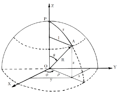
Figure 1: Geometrical sense of the line element coordinates Eqs. (8) and (9) for the case of the 2D spherical expanding space embedded in the 3D Euclidean space. The radius $R$ of the 2D sphere is the scale factor $R(t)=S(t)$ of the expanding 2D space. The “internal” metric distance between the galaxies $P$ and $A$ is $r$ and the “external” metric distance is $l$. The angle $\theta$ is the dimensionless comoving “distance” $\chi$.

In terms of the “external” metric distance $l(t)=S(t)\mu$ and dimensional comoving coordinate $\mu=I_{k}(\chi)$ (Fig. 1), the interval d$s$ has the form

$$ds^{\text{2}}=c^{\text{2}}dt^{\text{2}}-S^{\text{2}}(t)\frac{d\mu^{\text{2}}}{1-k\mu^{2}}-S(t)^{\text{2}}\mu^{\text{2}}(d\theta^{\text{2}}+\sin^{\text{2}}\theta d\phi^{\text{2}})\,.$$ (9)

The geometrical sense of these coordinates is given in Figs. 1 and 2 for the case of the expanding 2D spherical space embedded in the 3D Euclidean space. Here the radius $R$ of the 2D sphere is the scale factor $R(t)=S(t)$ and the angle $\theta$ is the dimensionless comoving “distance” $\chi$.

The relation between the internal and external distances

$$r(t)=S(t)\cdot\chi\,,\qquad l(t)=S(t)\cdot\mu$$ (10)

can be written as

$$r=S(t)I^{-1}_{\text{k}}(l/S)\,,\qquad l=S(t)I_{k}(r/S)\,,$$ (11)

where $I^{-1}_{k}$ is the inverse function for $I_{k}$. In the case of the flat universe ($k=0$) these distances coincide $r(t)=l(t)$.

Note that the exact general relativity expression for the space expansion velocity $V_{\text{exp}}$ is the time derivative of the metric distance given by Eq. (10), so that

$$V_{\text{exp}}(r)=\frac{dr}{dt}=\frac{dS}{dt}\chi=\frac{dS}{dt}\cdot\frac{r}{S}=H(t)r=c\frac{r}{R_{H}}\,.$$ (12)

The expression of $V_{\text{exp}}(z)$ is more complex and includes the distance–redshift relation $r(z)$. The derivation of the FLRW relations between metric$/$luminosity distances and redshift is given in Appendix B.

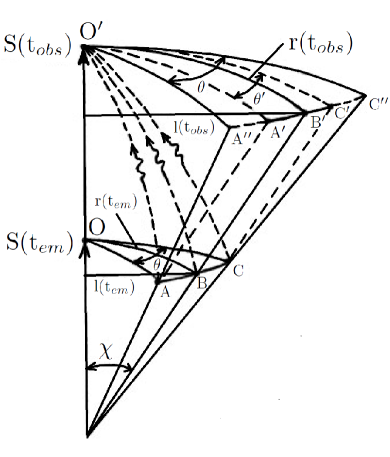
Figure 2: The 2D spherical expanding space embedded in the 3D Euclidean space. Metric distances at the times of emission $t_{\text{em}}$ and observation $t_{\text{obs}}$ of light from a distant galaxy have the linear size $ABC$. Note that $l(t_{\text{em}})$ and $r(t_{\text{em}})$ are the external and internal metric distances, respectively, when the scale factor is $S(t_{\text{em}})$.

2.2.2 Distance modulus, apparent and absolute magnitudes

The apparent stellar magnitude $m_{i}$ of an object observed through a filter “$i$” is defined via the ratio of the measured flux $F_{L,i}$ to the standard flux $F_{0}$. Taking into account Eq. (3) we can write

$$m_{i}=-2.5\log(F_{L,i}/F_{0})=5\log(d_{L})+25+M_{i}+C_{i}\,,$$ (13)

where $d_{L}$ is the luminosity distance measured in Mpc, $M_{i}$ is the absolute stellar magnitude of the standard source, and $C_{i}(z)=K_{i}+A_{i}+E_{i}$ involves different observational corrections, where the $K_{i},\,A_{i}$, and $E_{i}$ are redshift biases, extinction, and evolution corrections known for a standard candle class.

For the case of the bolometric fluxes $F_{L}$ and fluences $F_{E}$ given by Eqs. (3) and (4) we define the corresponding observed “distance modulus” as the luminosity distance modulus

$$\mu_{L}=\,m_{L}-M_{L}=5\log(d_{L})+25+C_{L,i}(z)\,,$$ (14)

and the energy distance modulus

$$\mu_{E}=\,m_{E}-M_{E}=5\log(d_{E})+25+C_{E,i}(z)\,.$$ (15)

To construct the HD we will fit observed flux and fluence distance moduli by the theoretical ones, which are given by Eqs. (48) and (50). Thus we get the HD as the ($\mu$ versus $z$) relations in two forms: for the measured flux $F_{L}$,

$$\mu_{L}=5\log(l(z)(1+z))+25=5\log l(z)+5\log(1+z)+25\,,$$ (16)

and for the measured fluence $F_{E}$,

$$\mu_{E}=5\log(l(z)(\sqrt{1+z})+25=5\log(l(z)+2.5\log(1+z)+25\,.$$ (17)

In fact for the SNe Ia observations we have measurements of the “luminosity distance modulus” $\mu_{L}(z)$. For GRB fluence, observations give the “energy distance modulus” $\mu_{E}(z)$. Hence, to construct the HD in terms of the GRB luminosity distance modulus $\mu_{L}$, Eq. (16), we must correct the GRB $\mu_{E}$ observational data by the factor

$$\mu_{L}=\mu_{E}+2.5\log(1+z)\,\,.$$ (18)

The correction Eq. (18) takes into account the additional factor $(1+z)$ in Eq. (3), which relates to the time dilation effect for the observed luminosity distance modulus of the GRBs.

2.3 Testing basic cosmological assumptions

Above, we considered three basic SCM principles, which include the geometrical gravity theory (general relativity), ECP of the strict mathematical homogeneity for the dynamically important matter, and the space expansion paradigm for the observed cosmological redshift.

In the spirit of practical cosmology the basic initial principles of the SCM must be tested with increasing accuracy and compared with other cosmological models at wider redshift intervals (Baryshev & Teerikorpi, 2012; Baryshev, 2015).

Here, for illustration of the HD predicted on the basis of different initial principles, besides SCM, we also consider the CSS, FF and TL models.

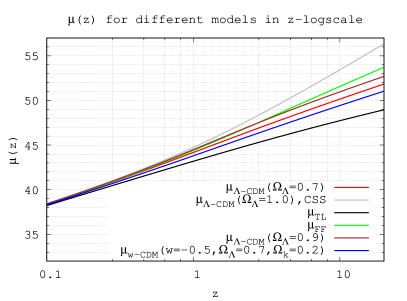
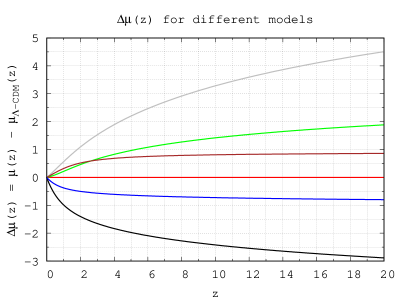
Figure 3: The luminosity distance modulus $\mu_{L}(z)$ for six considered cosmological models described in Sec.2.2 and Sec.2.3. Left: direct distance modulus, Right: residuals from the standard $\Lambda$CDM model.

2.3.1 The classical steady-state model

The classical steady state (CSS) model can be used for testing the perfect cosmological principle, which asserts that the observable universe is basically the same at any time and at any place, so that the matter density in the expanding universe remains unchanged due to a continuous creation of matter (Hoyle et al., 2000). The HD for the CSS has specific behaviour that can be directly tested by observations.

Theoretical parameters of the CSS model correspond to those of the zero-curvature Friedmann model with an exponentially growing scale factor $S(t)=S_{0}e^{Ht}$, ($H=H_{0}$ = const). The metric distance is

$$r^{\text{CSS}}(z)=l(z)=R_{H}\,z=r^{\text{Vac}}\,,$$ (19)

where $R_{H}=c/H_{0}$, and it is the same as in the pure vacuum $\Lambda$CDM model.

The luminosity distance modulus of the CSS model coincides with the $\Omega_{\Lambda}=1$ pure vacuum $\Lambda$CDM model:

$$\mu_{L}^{\text{CSS}}=5\log\,(R_{H}\,z)+\,5\log(1+z)+25+C_{i}(z)=\mu_{L}^{\text{Vac}}\,.$$ (20)

2.3.2 The field-fractal model

The field-fractal (FF) model can be used for testing three basic principles of the SCM – the gravity geometrization principle, the matter homogeneity principle, and the space expansion paradigm. The FF model is presented in Baryshev (2008) and Baryshev & Teerikorpi (2012) and its modern status allows one to formulate crucial observational tests, including the HD.

The FF model is based on the following basic assumptions: (1) the gravitational interaction is described by the Poincare–Feynman field gravitation theory in the flat Minkowski space-time, similar to all other fundamental physical interactions; (2) the total distribution of matter (visible and dark) is described by a fractal density law with the critical fractal dimension $D_{\text{crit}}=2$; and (3) the cosmological redshift has global gravitational nature within the fractal matter distribution.

An advantage of the FF model is that it solves the so-called Hubble–de Vaucouleurs paradox: the coexistence of the observed strongly inhomogeneous distribution of visible matter of the local Universe ($0.0003<z<0.03$) and the linear Hubble Law ($z=H\,r/c$) on the same scales  (Karachentsev et al., 2003; Baryshev & Teerikorpi, 2012). In the expanding space of the SCM the Hubble Law is a strict mathematical consequence of the homogeneous distribution of matter (ECP). So, starting from very small scales $\sim 1$ Mpc there must be a homogeneous substance, which has the density $\rho_{\text{dark}}\gg\rho_{\text{visible}}$.

In the FF model the linear Hubble redshift–distance law is consistent with the strongly inhomogeneous distribution of matter on small scales $1<r<100$ Mpc. Indeed, within a fractal galaxy distribution the global gravitational redshift of a source observed at a distance of $r$ will be $z_{\text{g}}\propto\phi(r)/c^{2}\propto M(r)/r\propto r^{D}/r\propto r^{1}$. Thus, it gives the linear redshift–distance law for the fractal dimension $D=2$. Taking into account the FF cosmological solution of the field equation for gravitational potential $\phi$, the redshift–distance relation is given by the following expression in Baryshev (2008) and Baryshev & Teerikorpi (2012):

$$z_{g}(x)=\left(\frac{1}{2\sqrt{x}}I_{1}(4\sqrt{x})\right)^{\frac{1}{2}}-1\equiv W(x)\,,$$ (21)

where $x=r/R_{H}$, $R_{H}=c/H_{\text{g}}$, and $I_{1}$ is the modified Bessel function. The corresponding metric distance–redshift relation is

$$r^{\text{FF}}(z)=R_{H}\,\,Y(z)\,,$$ (22)

where $Y(z)=W^{-1}(z)$ is the inverse function of $W(z)$. The properties of the gravitational redshift are analogous to those of the Doppler redshift and hence the luminosity distance modulus will be

$$\mu_{L}^{\text{FF}}=5\log\,(R_{H}\,Y(z))+\,5\log(1+z)+25+C_{i}(z)\,.$$ (23)

2.3.3 The tired-light model

The tired-light (TL) model in the Euclidean static space (e.g., La Violette, 1986) can be used as a toy model to demonstrate the importance of the time dilation cosmological effect. Within the framework of the TL model, the cosmological redshift is caused by the photon energy $E=h\nu$ decrease proportional to the covered distance, $h\nu_{\text{obs}}=Z\,h\nu_{\text{emit}}$, where $Z=e^{-\alpha r}$ is the Zwicky factor. Thus the distance–redshift relation is

$$r^{\text{TL}}(z)=R_{H}\,\ln{(1+z)}\,,$$ (24)

where $R_{H}=c/H_{\text{0}}$ and the luminosity distance modulus will be

$$\mu_{L}^{\text{TL}}=5\log\,(R_{H}\,\ln(1+z))+\,2.5\log(1+z)+25+C_{i}(z)\,.$$ (25)

2.3.4 Figures for considered models

In the context of SCM we consider the HD for three versions of the matter and dark energy density parameters: two $\Lambda$CDM models with $w=-1$ having $(\Omega_{\text{m}}=0.3;\,\,\Omega_{\text{vac}}=0.7;\,\,\Omega_{k}=0)$ and $(\Omega_{\text{m}}=0.1;\,\,\Omega_{\text{vac}}=0.9;\,\,\Omega_{k}=0)$, and $w$CDM model with $w=-0.5$ having $(\Omega_{\text{m}}=0.5;\,\,\Omega_{w}=0.7;\,\,\Omega_{k}=0.2)$. The metric and luminosity distances for these models are given by Eqs. (44), (45), and (48) and represented in Fig. 7. The luminosity distance modulus are given by Eq. (16) and represented in Fig. 3.

For all the considered models the relations between luminosity and metric distances are given in Table 1. The metric and luminosity distances as functions of redshift are represented in Fig. 7. The luminosity distance modulus for these models are represented in Fig. 3.

Model	$r(z)/R_{H}$	$d_{L}(z)/r(z)$	$d_{E}(z)/r(z)$
SCM	$\int 0^{z}\frac{dz^{\prime}}{h(z^{\prime})}$	$(1+z)$	$\sqrt{1+z}$
CSS	$z$	$(1+z)$	$\sqrt{1+z}$
FF	$Y(z)$	$(1+z)$	$\sqrt{1+z}$
TL	$\ln{(1+z)}$	$\sqrt{1+z}$	$\sqrt{1+z}$

Table 1: The dimensionless metric, luminosity and energy distances behaviour as functions of the redshift $z$ for the cosmological models described in Secs. 2.2 and 2.3.

3 LGRB as standard candles and Amati relation

3.1 The observed LGRB parameters

LGRB sources are related to explosions of massive core-collapse SN in distant galaxies (e.g., Woosley, 1993; Woosley & Bloom, 2006; Cano et al., 2017), though up to now there is no satisfactory theory of the LGRB radiation’s origin (Meszaros & Rees, 2014; Kumar & Zhang, 2015; Pe’er, 2015; Willingale & Mészáros, 2017). The observed LGRB photon spectrum is well approximated by the standard empirical model of Band et al. (1993)

$$N(E)\left[\frac{\text{photons}}{\text{keV~{}s~{}cm}^{2}}\right]=\begin{cases}AE^{\alpha}e^{-E/E_{0}},&E<(\alpha-\beta)E_{0}\\ BE^{\beta},&E>(\alpha-\beta)E_{0}\end{cases},$$ (26)

where $N\,(E=h\nu/100$ keV) is the Band function or the usual differential photon spectrum (d$N$/d$E$), $\alpha,\beta$ are observed the low-energy and high-energy spectrum parameters, $E_{0}$ is the break energy, $A$ is the normalized factor, and $B=A\,(\alpha-\beta)E_{0}\,\,e^{(\alpha-\beta)}$ is given from the smooth junction condition.

An important LGRB parameter is the observed peak energy $E_{\text{p}}$ (frequency) of the spectral energy distribution, i.e. the photon energy (frequency), at which the energy spectrum $\nu F_{\nu}=E^{2}N(E)$ is maximum. So, the rest-frame peak energy is

$$\qquad E_{\text{p},i}=E_{\text{p}}\,(1+z)\,.$$ (27)

The bolometric fluence (erg cm^-2) is calculated from observed values by the equation

$$S_{\text{bolo}}=F_{E}=S_{\text{obs}}\frac{\int_{\frac{1}{1+z}}^{\frac{10^{4}}{1+z}}E\,N(E)\text{d}E}{\int_{E_{\text{min}}}^{E_{\text{max}}}E\,N(E)\text{d}E}\,,$$ (28)

and the bolometric peak flux is

$$P_{\text{bolo}}=F_{L}=P_{\text{obs}}\frac{\int_{\frac{1}{1+z}}^{\frac{10^{4}}{1+z}}E\,N(E)\text{d}E}{\int_{E_{\text{min}}}^{E_{\text{max}}}N(E)\text{d}E}\,,$$ (29)

where $E_{\text{min}}$ and $E_{\text{max}}$ are the limits of the observed spectral energy range, and $P$ is in units [erg cm^-2 s^-1].

From Eq. (4) the isotropic radiated energy (erg) is given by the relation

$$E_{\text{iso}}=4\pi d_{E}^{2}S_{\text{bolo}}\,.$$ (30)

From Eq. (3) the isotropic peak luminosity (erg s^-1) is given by

$$L_{\text{p}}=4\pi d_{L}^{2}P_{\text{bolo}}\,.$$ (31)

3.2 Gravitational lensing and Malmquist biases

3.2.1 Observational distortion of theoretical LGRB parameters

There are a number of inevitable observational selection effects (e.g., limits on detector sensitivity, influence of the intervening matter, GL, and evolution), that potentially distort the measured flux and fluence, and hence the derived distance to a GRB. Thus the construction of the proper HD should take into account different selection and evolution effects, which have been widely debated in the literature (e.g., Schaefer, 2007; Liang et al., 2008; Wang & Dai, 2011; Dainotti et al., 2013b, a; Liu & Wei, 2015; Deng et al., 2016; Lin et al., 2016a, b; Wang et al., 2016, 2017; Demianski et al., 2017a; Lloyd-Ronning et al., 2019; Xue et al., 2019).

However, a definite answer to the role of selection effects in the LGRB luminosity estimation requires more data with known redshifts. The forthcoming THESEUS mission together with accompanying multimessenger observations is expected to bring a solution to this fundamental question.

3.2.2 Gravitational lensing along the LGRB line of sight

The apparent image of a distant source can be distorted by the GL effect of the mass density fluctuations (both visible and dark) along the line of sight. The GL of a variable source produces two main effects: it splits the source image and creates a time delay between different subimages of the source. According to modern observational surveys the GL plays an important role in cosmology. There is a sufficiently large probability for detection of strong lensing effects that allows one to study the total (dark and luminous) mass distribution of lenses (Ji et al., 2018; Acebron et al., 2020; Cervantes-Cota et al., 2020; Shajib et al., 2020). For GL of high-redshift LGRBs and quasi-stellar objects (QSOs), it is especially important to study protoclusters of low-luminosity star-forming galaxies, which were recently discovered at $z\approx 6.5$ (Calvi et al., 2019).

The next generation of cosmological surveys will elucidate the value of weak and strong lensing biases in the true luminosity of distant sources and hence in observed magnitude–redshift relations at $z\sim 1$ (Laureijs et al., 2011; Scolnic et al., 2019; Cervantes-Cota et al., 2020).

Basic physics of the GLB. Flux magnification of the split images due to GL should be taken into account in observations of distant compact sources, such as SNe, GRBs and QSOs. For the lens mass $M<10^{8}$ $M_{\odot}$ the splitting angle is $\theta<0.3$ arcsec and a compact source will be observed as one image (for ordinary angular resolution). This gravitational magnification of the observed fluxes will lead to the GLB in the estimated luminosity of compact sources.

GL along a GRB line of sight magnify its flux due to different gravitating structures of the Universe, such as dark and luminous stellar mass objects, globular and dark stellar mass clusters, and galaxies and dark mass galaxy halos. Hence the GL can have a great impact on high-redshift LGRBs.

For estimation of the GLB one must assume a GL model that includes three parts: (1) a lensed object (source); (2) lensing objects (lenses); and (3) a distribution of lenses along the source line of sight. As a source, we consider distant SNe Ia, GRBs, and QSOs.

The lensing object (gravitational lens) is defined by its mass density distribution. In accordance with the total lens mass interval, usually one considers three types of lensing: microlensing ($M<10^{3}$ $M_{\odot}$), mesolensing ($10^{3}<M<10^{8}$ $M_{\odot}$) and macrolensing ($M>10^{8}$ $M_{\odot}$). Gravitational lenses include both visible and dark matter objects. Examples are stars, stellar clusters, galaxies and galaxy clusters. The transparent gravitational lenses (like globular clusters and dwarf galaxies) have a larger cross-section for lensing effect due to the more complex structure of caustics.

A very important part of the GL model is the assumed distribution of lenses along the line of sight. It plays a crucial role in the magnification probability and hence in the GLB. The strongly inhomogeneous distribution of matter along the line of sight leads to a larger lensing probability than the usually considered homogeneous distribution of matter (due to lens clustering). Observational data on the large-scale structure of the local and distant Universe reveal inhomogeneous (fractal-like) visible distribution of matter within scales larger than hundreds of megaparsecs (Gabrielli et al., 2005; Baryshev & Teerikorpi, 2012; Courtois et al., 2013; Einasto et al., 2016; Lietzen et al., 2016; Shirokov et al., 2016; Tekhanovich & Baryshev, 2016).

Gravitational mesolensing of QSOs by globular clusters was considered by Baryshev & Ezova (1997), taking into account the fractal distribution of matter along the line of sight. They demonstrated that the King-type transparent lenses (which have additional conic caustics) together with fractal large-scale distribution of the lenses along the line of sight (which enhance the total cross-section) will essentially increase the lensing probability.

Another evidence for mesolensing was found by Kurt & Ougolnikov (2000) and Ougolnikov (2001) in the Burst and Transient Source Experiment (BATSE) catalogue, where there are several GRB candidates that are probably lensed by intergalactic globular clusters.

Weak and strong GL. There are many papers considering the weak and strong gravitational lensing effect for SN Ia, LGRB and QSO observations (Holz & Wald, 1998; Wang et al., 2002; Holz & Linder, 2005; Jönsson et al., 2008; Jönsson et al., 2010; Wang & Dai, 2011; Smith et al., 2014; Ji et al., 2018; Scolnic et al., 2019; Cervantes-Cota et al., 2020).

The light from distant compact sources is affected by the GL induced by inhomogeneous massive structures (visible and dark) of the Universe. Since photons are conserved by the lensing, the mean flux over the sources is preserved. The observed flux can be magnified (or reduced) by the GL produced by random mass fluctuations in the intervening matter distribution. This effect leads to an additional dispersion in GRB brightness. The probability distribution function (PDF) of GL magnification has higher dispersion than a Gaussian distribution (Valageas, 2000; Wang et al., 2002; Oguri & Takahashi, 2006).

A statistical approach for taking into account weak GLB and MB in the LGRB observations was suggested by Schaefer (2007). It was developed by Wang & Dai (2011), where a sample of 116 LGRBs was analysed. They found that weak GLB effect shifts the estimation of matter density to lower values. So $\Omega_{\text{m}}$ shifts from 0.30 to 0.26 and the corresponding vacuum density $\Omega_{\Lambda}$ shifts from 0.70 to 0.74.

However, as emphasized in Scolnic et al. (2019) and Cervantes-Cota et al. (2020), one of the most important problems of the next generation cosmological measurements is the theoretical uncertainty in the expected lensing magnification bias. It is still one of the largest unknown systematic effects, as the lensing probability is sensitive to both large- and small-scale distribution of matter that is difficult to model. The forthcoming space missions, such as Euclid, will allow one to estimate the value of weak and strong lensing biases in the magnitude–redshift relations at $z\sim 1$ (Laureijs et al., 2011) and beyond (Calvi et al., 2019).

In particular, the mesolensing and strongly inhomogeneous line of sight distribution of matter can lead to essential changes in the estimated cosmological density parameters. We started the observational program for optical study of the LGRB line-of-sight distribution of lensing galaxies using photometric and spectral galaxy redshifts (e.g., Castro-Tirado et al., 2018; Sokolov et al., 2018b; Sokolov et al., 2018a). Observations of deep fields in the directions of LGRBs reveal galaxy clusters along the LGRB line of sights. This program is important for estimation of GLB in LGRB catalogues.

Malmquist bias (MB). The GL of LGRBs produces apparent increase of flux $P_{\text{bolo}}$ and fluence $S_{\text{bolo}}$ due to the gravitational lens magnification, which does not change frequency (i.e., the peak energy $E_{\text{p}}=h\nu_{\text{p}}$) of the lensed radiation. This can be misinterpreted as an evolution of the GRB luminosity.

If we take into account that there is a threshold for the detection in the burst apparent brightness, then, with GL, bursts just below this threshold might be magnified in brightness and detected, whereas bursts just beyond this threshold might be reduced in brightness and excluded. This observational selection effect is known as the Malmquist bias (MB) that plays an important role in observational cosmology (Baryshev & Teerikorpi, 2012).

Schaefer (2007) considered the GLB and the MB effects for a sample of 69 LGRBs. He found that the GLB and MB are smaller than the intrinsic error bars. However, as we emphasized above, modern observations reveal strong matter clustering and so more complex lensing models must be studied further. Note that for THESEUS observations the MB will be shifted to larger distances due to better sensitivity.

Phenomenological model for GLB and MB. The crucially important fundamental question on the role of the GLB in high-redshift SN Ia, LGRB and QSO data is still open and needs additional observational and theoretical studies. Detailed observational study of the GLB is one of the primary tasks of future ground-based and space missions. However, already now, we can estimate quantitatively the value of combined contribution of the weak and strong GL effect and the MB, if we introduce simple parametrization of the observed radiation flux from a distant source.

Let one consider a phenomenological approach to the study of LGRB GL and bias. It can be considered as the first step in taking into account the common action of the GLB and MB, together with the strongly inhomogeneous distribution of lenses along the line of sight. Consider a general bolometric fluence correction in the power-law form

$$\qquad S_{\text{bolo}}^{\text{cor}}=\frac{S_{\text{bolo}}}{(1+z)^{k}}\,,$$ (32)

where $S_{\text{bolo}}$ is the observed bolometric fluence, k is the corresponding bias parameter, which parametrizes the strength of the apparent fluence magnification. According to Eq. (32) the true value of GRB fluence $S^{\text{true}}_{\text{bolo}}=S^{\text{cor}}_{\text{bolo}}$ and it must be used to compare theory with observations.

Note, that according to Deng et al. (2016) there is an observed evolution of the intrinsic peak luminosity of the high-redshift LGRBs in the form $L_{\text{p}}\propto(1+z)^{k_{\text{p}}}$ with $k_{\text{p}}=1.49\pm 0.19$. It is clear that at least a part of this “evolution” can be caused by the GLB$+$MB selection effects.

As a testing value of the GLB$+$MB parameter, we consider $k=0.25,\,0.5$, and $0.75$ in Eq. (32), which is less than the observed luminosity increase power-law exponent $k_{\text{p}}=1.49$ in Deng et al. (2016).

The solution of the fundamental problem (derivation of the true value of the GLB and MB parameter $k$) will be based on future combined development of both lensing models (magnification PDF) and observations of inhomogeneous distribution of lenses along the LGRB line of sight. However now, using our phenomenological model, we can estimate the restrictions that follows from GLB and MB on the LGRB magnitude–redshift relation. Then we can compare the theoretical cosmological model predictions with observational data corrected by the bias.

3.3 Amati relation

LGRBs can be used as standard candles due to the relation discovered for GBRs from BeppoSAX observations. The correlation between the observed photon energy (frequency) of the peak spectral flux $E_{\text{p},i}$, which corresponds to the peak in the $\nu F_{\nu}$ spectra, and the isotropic equivalent radiated energy $E_{\text{iso}}$ was discovered and studied by Amati et al. (2002, 2008) and Amati & Della Valle (2013). The Amati relation can be written as

$$\log{\frac{E_{\text{iso}}^{\text{A}}}{\text{1 erg}}}=a\log{\frac{E_{\text{p},i}}{\text{300 keV}}}+b\,,$$ (33)

where $E_{\text{p},i}$ is the GRB source rest-frame spectrum peak energy given by Eq. (27), “$a$” and “$b$” are Amati parameters.

The Amati correlation can be established for a sample of GRBs where redshifts $z$ are measured. Additionally, the Amati coefficients can be calibrated by GRBs in the same range, where we have good statistic of SNe Ia and where we approximate the $d_{L}(z)$ – luminosity distance as a function of redshift.

3.4 Extended Amati relation

The Amati relation (Eq. 33) can be transformed into an extended Amati relation (the Amati law of GRB distances) by using Eqs. (3), (4), (48), and (50) so the GRB luminosity distance is given by the equation

$$d_{L}^{\text{A}}\,[\text{cm}]=\left(\frac{(1+z)E_{\text{iso}}^{\text{A}}(E_{\text{p},i})}{4\pi S_{\text{bolo}}}\right)^{\frac{1}{2}}\,\,.$$ (34)

Taking into account Eq. (32) we get the GRB luminosity distance modulus in the form

$$\mu^{\text{A}}_{\text{GRB}}=25+\frac{5}{2}\left[\log{\frac{(z+1)^{k+1}}{4\pi S_{\text{bolo}}}+a\log{E_{\text{p},i}}+b}\right]\,,$$ (35)

where $a,\,b$ are the Amati coefficients, and k is the parameter of the GLB and MB. Hence the correction of the joint distance modulus due to action of GLB and MB is

$$\Delta\mu_{\text{eff}}=2.5\log{(z+1)^{k}}\,,$$ (36)

where the parameter k is a measure of the observed HD distortion by the GLB and MB effects.

4 SN Model-Independent Hubble Diagram

The SNe Ia model-independent HD can be directly inferred from the Pantheon observational data (Scolnic et al., 2018), including 1 048 SNe Ia. It is shown in Fig. 4 (left). The luminosity distance values $d_{L}$ and the luminosity distance modulus $\mu=m-M$ are given by the relation

$$\mu_{L}^{\text{SN}}=5\log{\frac{d_{L}^{\text{SN}}(z)}{\text{Mpc}}}+25\,,$$ (37)

where the luminosity distance is expressed in megaparsecs for the given $z$.

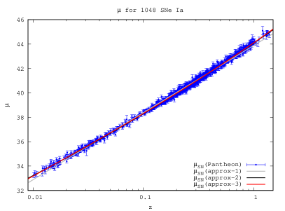
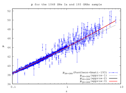
Figure 4: The model-independent Hubble diagram (HD) for Pantheon SNe Ia (left) and for combined SNe Ia$+$LGRB (right) and its polynomial approximations.

If the parameters are determined using some cosmological model with adjusted fixed parameters, giving the dependence $d_{L}(z)$, then the HD obtained for GRBs cannot be correctly used to determine both the cosmological model and its parameters, since this approach involves the circularity problem (e.g., Kodama et al., 2008).

Instead, the task is to determine the dependence $d_{L}(z)$ for GRBs without making assumptions about cosmology (at least in the first approximation). To construct the $d_{L}(z_{i})$ we use the Pantheon observational data on $\mu(z_{i})$ with errors in determining the distance modulus and effects of deviations from the standard candles. Index $i$ is indicated in the process of discreteness. The continuous function $d_{L}(z)$ must be smooth and monotonically increasing.

Without resorting to cosmology assumptions, we can approximate the dependence $d_{L}(z)$ in the logarithmic coordinates by some elementary mathematical function by the least-square method. Since the dependence $\mu(\log{z})$ is linear at small $z$, it is reasonable to approximate it with polynomials of small degree $n$, i.e.

$$\mu(x)\approx P_{n}(x)=\sum_{i=0}^{n}p_{i}x^{i}\,,$$ (38)

where $x=\log{z}$.

The function is linear for parameters, hence it is possible to apply the matrix least-squares method. In turn, the approximation of the dependence $d_{L}(z)$ will be exponential to the polylogarithmic function

$$d_{L}(z)\,[\text{Mpc}]\approx 10^{0.2P_{n}(x)-5}\,.$$ (39)

In this approach, we use the weighted least-squares method to minimize

$$\chi^{2}=\sum_{i=1}^{N}w_{i}(y_{i}-P_{n}(x_{i}))^{2}\,,$$ (40)

where $x_{i}=\log z_{i}$, $y_{i}=\mu_{i}$, and $w_{i}=1/\sigma^{2}_{\mu_{i}}$ for each $i$ of $N$ SNe Ia by calculating the coefficients of the polynomial $P_{n}$ and their errors.

Calculations were made for polynomials of degree $1-3$, the results are shown in Table 2. Approximations of Eq. (38) are shown in Fig. 4. The linear approximation is a good fit for small redshifts and the differences between polynomials of degrees $2$ and $3$ are small.

Sample	Degree	$p_{0}$	$p_{1}$	$p_{2}$	$p_{3}$
	1	$43.88\pm 0.02$	$5.50\pm 0.01$	–	–
Pantheon	2	$44.08\pm 0.01$	$6.15\pm 0.03$	$0.36\pm 0.02$	–
	3	$44.10\pm 0.01$	$6.28\pm 0.07$	$0.57\pm 0.09$	$0.08\pm 0.03$
	1	$43.896\pm 0.000$	$5.520\pm 0.000$	–	–
SNe+LGRBs	2	$44.062\pm 0.000$	$6.096\pm 0.002$	$0.341\pm 0.001$	–
	3	$44.063\pm 0.000$	$6.099\pm 0.005$	$0.347\pm 0.011$	$0.003\pm 0.002$

Table 2: The best approximation coefficients (Eq. 38) of the luminosity distance modulus $\mu(\log{z})$ for the Pantheon SNe Ia ($z_{\text{cmb}}$) and LGRB samples.

The polynomials can be used for the junction condition between SNe Ia and LGRB data in the interval $0.01<z<1.0$, where cosmological and selection effects are small. In Fig. 4, we also show the polynomial approximation of our total sample of SNe Ia and LGRBs for the total redshift interval $0.1<z<10$.

5 LGRB Hubble Diagram for different cosmological models

The cosmological models considered in Sec.2 cover a wide interval of deflections from the standard $\Lambda$CDM theoretical predictions for the luminosity distance modulus. Now we take the LGRB data to perform the high-redshift test of these models.

5.1 LGRB sample

We use the LGRBs sample of Amati et al. (2019) for which there is a table of calculated luminosity distance moduli for total redshift interval.

As we emphasized above, the Hubble law of linear distance–redshift relation starts immediately beyond the border of the Local Group (Karachentsev et al., 2003). However there are a small number of LGRBs at redshifts $z<1$. This is why we have to use the SNe Ia observations, which give reliable luminosity distance–redshift data up to redshifts $\sim 1$. The LGRB data that have a common region of redshifts with the SN data must obey the junction condition, which is fulfilled for our sample.

5.2 Results for different assumed basic cosmological relations

In Figure 5 (and in Fig. 8), we present the LGRB HDs for the total 1 048 SN Ia plus 193 LGRBs of the Amati et al. (2019) sample. Theoretical models were calculated for the flat $\Lambda$CDM with $\Omega_{\Lambda}=0.7,\,0.9$, and $1.0$; the $w$CDM with a positive curvature having $w=-0.5$, $\Omega_{\Lambda}=0.7$, and $\Omega_{k}=0.2$. Different basic cosmological assumptions are illustrated by calculations of the luminosity distance modulus for CSS, FF and TL models (Sec. 2). The Hubble parameter is $h=0.7$ for all models.

Figure 5 demonstrates the SNe Ia and LGRB data in the linear redshift scale without taking into account the GLB and MB ($k=0$ in Eq. 32) and an example with the parameter $k=0.5$, which takes into account the possible GLB and MB. The deviations of the luminosity distance moduli and of the linear scale median values ($\Delta z=0.3$) of the LGRB sample from the standard $\Lambda$CDM model are also shown. Figure 8 shows the same data but in logarithmic scale and with the logarithmic scale median values ($\Delta\log{z}=0.1$) of the LGRB sample. The blue points mean median values at $z<0.35$ and $4.2<z$, respectively. The legend in all plots is the same.

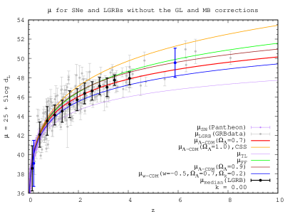
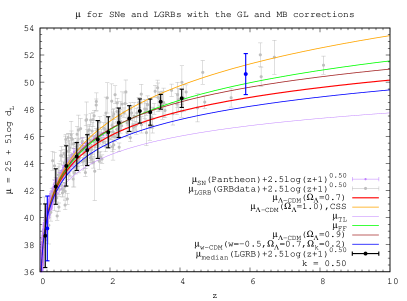
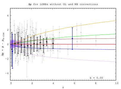
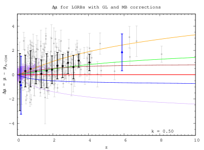
Figure 5: Top panels: the observed luminosity distance modulus $\mu$ versus redshift (HD) in linear $z$-scale for the SN Ia and LGRB samples. Black points are the median values of $\mu$ with linear step $\Delta z=0.3$ for the LGRB sample. Bottom panels: the residuals $\Delta\mu$ from the standard $\Lambda$CDM model for the observed luminosity distance modulus. Left: without the correction for the GLB and MB. Right: corrected with $k=0.5$. The colour curves correspond to the cosmological models defined in Section 2.

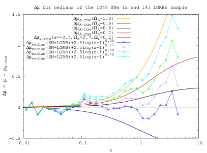
Figure 6: The residuals $\Delta\mu$ from the standard $\Lambda$CDM model for the observed luminosity distance modulus $\mu$ calculated for different values of the GLB and MB parameter $k=0.00,\,0.25,\,0.50$, and $0.75$. The colour curves correspond to the standard cosmological models (SCMs) with $\Omega_{\Lambda}=0.7,\,0.8,\,0.9$, and $1.0$ and positive curvature $w$CDM model with $w=-0.5$, $\Omega_{\Lambda}=0.7$, and $\Omega_{k}=0.2$ defined in Section 2.

To illustrate different values of the parameter $k$, in Figure 6, we present the results in residual form for the cases $k=0.0,\,0.25,\,0.50$, and $0.75$. We also consider three simple statistical measures of the $\chi^{2}$ test in form from Pearson & Hartley (1957, p. 13). The first statistic uses all LGRB sample points,

$$\chi^{2}_{1}=\sum_{i=1}^{N_{\text{GRB}}}\frac{(\mu_{i}-\mu_{\text{model}})^{2}}{\mu_{\text{model}}}\,,$$ (41)

where $N_{\text{GRB}}$ is the GRB number in each sample, $\mu_{i}$ is the GRB distance modulus, and $\mu_{\text{model}}$ is the considered cosmological model distance modulus at the same redshift $z_{i}$.

The second one uses the uniform linear median values for bins,

$$\chi^{2}_{2}=\sum_{j=1}^{N_{\text{bins}}}\frac{(\mu_{j}-\mu_{\text{model}})^{2}}{\mu_{\text{model}}}\,,$$ (42)

where $N_{\text{bins}}$ is the number of bins in each sample, $\mu_{j}$ is the median distance modulus, and $\mu_{\text{model}}$ is the cosmological model distance modulus at the same redshift $z_{j}$.

The third one uses the uniform logarithmic scale median values for bins,

$$\chi^{2}_{3}=\sum_{k=1}^{N_{\text{bins}}}\frac{(\mu_{k}-\mu_{\text{model}})^{2}}{\mu_{\text{model}}}\,,$$ (43)

where $N_{\text{bins}}$ is the number of bins in each sample, $\mu_{k}$ is the uniform in logarithmic scale median distance modulus, and $\mu_{\text{model}}$ is the cosmological model distance modulus at the same redshift $z_{k}$.

The results of our calculations of the statistics for the original and corrected (for GL and MB effects) LGRB sample of Amati et al. (2019) are represented in Table 3. The detailed description of the models is given in Sec. 2 and Sec. 3.

From Table 3 we can see that uncorrected LGRB data correspond better to the standard parameters of the $\Lambda$CDM model (see the column for $\Omega_{\Lambda}=0.7$). Whereas the GLB and MB shift the fit towards the $\Lambda$CDM model with $\Omega_{\Lambda}=0.9$ for $k=0.5$. Among alternative cosmological assumptions the corrected LGRB data are consistent with the field-fractal model (column FF), but reject the tired-light model (column TL) .

$\sqrt{\chi^{2}}$	$k$	$\Lambda$CDM($\Omega_{\Lambda}=1.0$)	FF	$\Lambda$CDM($\Omega_{\Lambda}=0.9$)	$\Lambda$CDM($\Omega_{\Lambda}=0.7$)	$w$CDM($w=-0.5,~{}\Omega_{\Lambda}=0.7,~{}\Omega_{k}=0.2$)	TL
$\chi_{1}$	0.00	3.051	2.405	2.411	2.302	2.572	3.735
$\chi_{2}$	0.00	0.611	0.289	0.295	0.152	0.293	0.742
$\chi_{3}$	0.00	0.553	0.274	0.280	0.140	0.237	0.623
$\chi_{1}$	0.25	2.702	2.290	2.295	2.425	2.884	4.219
$\chi_{2}$	0.25	0.461	0.171	0.181	0.223	0.438	0.899
$\chi_{3}$	0.25	0.424	0.166	0.175	0.180	0.359	0.759
$\chi_{1}$	0.50	2.441	2.321	2.325	2.674	3.273	4.728
$\chi_{2}$	0.50	0.317	0.153	0.165	0.354	0.589	1.057
$\chi_{3}$	0.50	0.298	0.130	0.141	0.287	0.490	0.896
$\chi_{1}$	0.75	2.298	2.491	2.494	3.018	3.716	5.255
$\chi_{2}$	0.75	0.191	0.257	0.265	0.501	0.743	1.215
$\chi_{3}$	0.75	0.186	0.207	0.214	0.412	0.623	1.034

Table 3: The $\chi_{1}$, $\chi_{2}$, and $\chi_{3}$ statistics for the LGRB sample fitting by considered cosmological models (Section 2).

6 Discussion and conclusions

Modern astrophysical facilities open new possibilities for testing the basis of the cosmological models by using the observational approach to cosmology developed by Hubble–Tolman–Sandage in the 20th century. In the beginning of the 21st century the multimessenger astronomy allows one to test the fundamental initial assumptions of cosmological models with a higher accuracy and in a very wide redshift interval up to $z\sim 10$, instead of $z\sim 0.003$ in the first cosmological observations.

The high-redshift HD for LGRBs can be used as a necessary condition for plausibility of a cosmological model, because it can test the directly observed flux–distance–redshift relation. In Section 2 we considered several examples of the cosmological $\mu\,\text{vs}\,z$ relations (the HD), which correspond to specific initial assumptions in the cosmological models.

Existing LGRB data demonstrate that the Amati relation can be used for construction of the observed HD at the model-independent level, hence it is useful for testing theoretical models. However, the main uncertainty when comparing the observational HD and the theoretically predicted $\mu\,\text{vs}\,z$ relation is the problem of observational data distortion by different kinds of evolution and selection effects.

As emphasized in Scolnic et al. (2019), and Cervantes-Cota et al. (2020), one of the most important problems of the next generation cosmological measurements is the theoretical uncertainty in the expected lensing magnification bias. It is still one of the largest unknown systematic effects, as the lensing probability is sensitive to both large- and small-scale distribution of matter for which there is no analytical model. So this crucially important fundamental question on the role of the GLB in high-redshift SN Ia, LGRB and QSO data is still open and needs more observational and theoretical studies.

Thus, an important obstacle for derivation of true cosmological parameters from the high-redshift LGRB HD is to correctly account for the GL. Flux magnification and MB play a crucial role in comparison of different cosmological models. For example, “observed” evolution of the LGRB peak luminosity $L_{\text{p}}\propto(1+z)^{k_{\text{p}}}$ (Deng et al., 2016) can be partly caused by the GLB and MB.

In a previous study of the LGRB weak lensing statistical effects (Schaefer, 2007; Wang & Dai, 2011) an analytical lensing model was developed for calculation of the distance dispersion from the universal probability distribution function. Modern observational data reveal a very complex large-scale distribution of matter (dark and luminous), which is difficult to model (Scolnic et al., 2019), but which can essentially change the probability of the GL. Especially for the high-redshift LGRBs, there is an important additional contribution to the lensing bias from the recently discovered population of protoclusters of low-luminosity star-forming galaxies at redshifts $z\sim 6$ (Calvi et al., 2019).

In our paper, as the first step for a quantitative examination of the possible lensing effects, we introduce a phenomenological one-parameter $k$-model (Section 3.2.2). In this way one can estimate the total GL effect produced by a combination of weak and strong lensing together with the MB. Though such an approach does not allow one to study the relative contributions and redshift evolution of these parameters, it gives the possibility to get restrictions on the considered cosmological models.

We extend the Wang & Dai (2011) findings of a small shift of $(\Omega_{\text{m}},\,\Omega_{\Lambda})$ by the weak GL. Our simple lensing model phenomenologically describes the total bias due to strong and weak GL together with the strong inhomogeneous distribution of lenses along the LGRB line of sight (Section 3.2.2).

According to our analysis of the sample of 193 LGRBs (Amati et al., 2019), we conclude that the high-redshift HD, corrected for the GLB and MB effects by the parameter $k$, points to a tendency to more vacuum-dominated $\Lambda$CDM models: for $k\rightarrow 0.5$ we get $\Omega_{\Lambda}\rightarrow 0.9$ and $\Omega_{\text{m}}\rightarrow 0.1$ (see Figs. 5 and 8). It is interesting to note that our results show that the positive curvature $w$CDM model with $w=-0.5$, $\Omega_{\Lambda}=0.7$, and $\Omega_{k}=0.2$ does not pass the HD test for all values of the bias parameter $k$.

Existing LGRB observations in the redshift interval 1–10 allow one to get new restrictions on several examples of alternative theoretical flux–distance–redshift relations considered in Sec.2. We showed (see Fig. 6 and Table 3) that the high-redshift LGRB HD, corrected for the GLB and MB effects, could be consistent with the CSS model if $k\rightarrow 0.75$. It is also compatible with the FF cosmological model for $k\rightarrow 0.5$, but it rejects the TL assumption for all values of the bias parameter $k$.

Derivation of the true value of the GL and MB parameter $k$ will be based on the future development of both lensing models and observations of the inhomogeneous distribution of lenses along the LGRB line of sight. The forthcoming space missions, such as Euclid, will elucidate the value of weak and strong lensing biases in the magnitude–redshift relations at $z\sim 1$ (Laureijs et al., 2011).

Future THESEUS space observations of GRBs and accompanying multimessenger ground-based studies, including large [in particular Gran Telescopio Canarias (GTC), Bolshoi Teleskop Alt-azimutalnyi (BTA), and Elbrus-2] and even 1-m class optical telescopes can be used as a powerful tool for testing the basic cosmological principles. In particular, we started the program for optical study of the LGRB line-of-sight distribution of lensing galaxies (Castro-Tirado et al., 2018; Sokolov et al., 2018a; Sokolov et al., 2018b).

The THESEUS GRB mission will provide several hundreds of LGRBs with measured redshifts and spectral peak energy $E_{\text{p}}$ and together with optical line-of-sight observations will allow one to take into account the GLB and MB. This opens new possibilities for using the LGRB HD for checking the basic assumptions of cosmology, a prerequisite for establishing the observationally based true world model.

Appendix A abbreviations

• HD – Hubble diagram

• SN(e) – supernova(e)

• GRB(s) – gamma-ray burst(s)

• LGRB(s) – long gamma-ray Burst(s)

• FLRW – Friedmann–Lemaitre–Robertson–Walker

• SCM – standard cosmological model

• THESEUS – Transient High-Energy Sky and Early Universe Surveyor (space mission)

• Euclid – space mission

• MB – Malmquist bias

• GL – gravitational lensing

• GLB – gravitational lensing bias

• GRT – general relativity theory

• ECP – Einstein’s cosmological principle

• EoS(s) – Equation of state(s)

• CSS – classical steady-state model

• FF – field-fractal model

• TL – tired-light model

• QSO(s) – quasi-stellar object(s)

  Appendix B Metric and luminosity distances

  B.1 Metric distance–redshift relations

  There are two kinds of metric distance in the FLRW model. The internal metric distance $r$ between the observer and the source at redshift $z$ at cosmic time $t=t_{0}$ in general expanding space models is given by the relation

  $$r(t_{0},z)=r(z)=\frac{c}{H_{0}}\int_{0}^{z}\frac{\text{d}z^{\prime}}{h(z^{\prime})}\,,$$ (44)

  and the external metric distance $l$ will be

  $$l(t_{0},z)=l(z)=S(t_{0})I_{k}(r(z)/S(t_{0}))\,,$$ (45)

  where the scale factor at present epoch $S(t_{0})=S(0)=c/H_{0}(k/\Omega_{k})^{\text{1/2}}$. Here the normalized Hubble parameter $h(z)=H(z)/H_{0}$ in the case of the $w$CDM model, having two fluids with equations of state for cold matter $p=0$ and for quintessence (dark energy) $p=w\rho c^{2}$ ($w<0$), is given by Friedmann’s equation as

  $$h(z)=\sqrt{\Omega^{0}_{\text{m}}(1+z)^{3}+\Omega^{0}_{\text{DE}}(1+z)^{\text{3(1+w)}}-\Omega^{0}_{k}(1+z)^{2}}\,,$$ (46)

  where density parameters are defined as $\Omega_{i}=\rho_{i}/\rho_{\text{c}}$ with the critical density $\rho_{\text{c}}=3H^{2}/8\pi G$, and $w$ is the dark energy equation of state (EoS) parameter.

  The curvature density parameter is $\Omega_{k}=kc^{2}/S^{2}H^{2}=(\Omega_{\text{tot}}-1)$. We use the definition of $\Omega_{k}$ that has the same sign as the curvature constant ${k}$. Note that in a number of papers they use another definition $\bar{\Omega}_{k}=-\Omega_{k}$ so the negative curvature space has a positive bar curvature density parameter.

  In the general case of several non-interacting fluids $\rho_{i}$ with EoSs $p_{i}/\rho_{i}c^{2}=\alpha_{i}$, the total density parameter is $\Omega_{\text{tot}}=\Sigma_{i}\Omega^{0}_{i}(1+z)^{3(1+\alpha_{i})}$. For $w=-1$ we have $p=-\rho$ and constant cosmological vacuum density: $\Omega_{\Lambda}=\Omega^{0}_{\text{DE}}$ = const, which is called the $\Lambda$CDM model. For dark energy parameter $w<0$ the model is called quintessence $w$CDM, and for $w<-1$ we have the “phantom” model.

  B.2 Luminosity and energy distances

  Consider a light source at the metric distance $r(t_{0},\chi)=S(t_{0})\chi$ detected at the time $t=t_{0}$ in the Friedmann universe.

  The source emitted light at the time $t=t_{1}$ isotropically around it with the bolometric (total) luminosity $L_{\text{iso}}$ (erg s^-1). Draw a sphere with the source in the centre and the observer at the surface at the moment of reception ($t=t_{0}$).

  The area of the sphere is $4\pi(S(t_{0})\mu)^{2}=4\pi l^{2}(z)$. According to Eq. (3), for the source isotropic luminosity $L_{\text{iso}}$ we measure the bolometric flux $F_{L}$ at luminosity distance $d_{L}$ as

  $$F_{L}\left[\frac{\text{erg}}{\text{s~{}cm}^{2}}\right]=\frac{L_{\text{iso}}}{4\pi l^{\text{2}}(z)(1+z)^{\text{2}}}=\frac{L_{\text{iso}}}{4\pi d_{L}^{2}(z)}\,.$$ (47)

  Here two factors $(1+z)$ take into account the observed energy decrease and time dilation effects. Hence the luminosity distance $d_{L}$ in the Friedmann’s models is defined according to Eq. (45) as

  $$d_{L}(z)=(1+z)\,l(z)=\frac{c}{H_{0}}\frac{(1+z)}{\sqrt{|\Omega^{0}_{\text{k}}|}}I_{k}\left(\sqrt{|\Omega^{0}_{\text{k}}|}\int_{0}^{z}\frac{\text{d}z^{\prime}}{h(z^{\prime})}\right)\,,$$ (48)

  where $\Omega^{0}_{k}$ is the curvature density parameter, and $I_{k}(x)=\sinh(x)$ for $\Omega_{k}<0,I_{k}(x)=x$ for $\Omega_{k}=0$, and $I_{k}(x)=\sin(x)$ for $\Omega_{k}>0$. The metric and luminosity distances for the models from section 2.3.4 are given by equations (44), (45), and (48) and represented in Fig. 7.

  For the total source bolometric energy $E_{\text{iso}}$ (erg) we measure the fluence $F_{E}$ (erg cm${}^{-2})$ at “energy distance” $d_{E}$, so we get from Eq. (4),

  $$F_{E}\left[\frac{\text{erg}}{\text{cm}^{2}}\right]=\frac{E_{\text{iso}}}{4\pi l^{\text{2}}(z)(1+z)}=\frac{E_{\text{iso}}}{4\pi d_{E}^{2}(z)}\,,$$ (49)

  where the factor $(1+z)$ takes into account the energy decreases, and from Eq. (45) we get the expression for the energy distance in the form

  $$d_{E}(z)=\sqrt{(1+z)}l(z)=\frac{c}{H_{0}}\frac{\sqrt{(1+z)}}{\sqrt{|\Omega^{0}_{k}|}}I_{k}\left(\sqrt{|\Omega^{0}_{k}|}\int_{0}^{z}\frac{\text{d}z^{\prime}}{h(z^{\prime})}\right)\,.$$ (50)

  The Hubble radius is $R_{{H}_{0}}=c/H_{0}\approx 4\,286\,h^{-1}_{\text{70}}$ Mpc. According to recent Planck results, which probe the redshift $z\sim 1\,000$, the primary cosmological parameters are the curvature parameter $\Omega_{k}=-0.0007\pm 0.0012$ (in our definition $\Omega_{k}$ has the same sign as the curvature constant $k$), the EoS parameter $w=-1.03\pm 0.03$, and the Hubble parameter $H_{0}=67.4\pm 0.5$ km s^-1 Mpc^-1 (Aghanim et al., 2018).

  However, recent local measurements of the HD give the $H_{0}=74.03\pm 1.42$ km s^-1 Mpc^-1, which points to some new physics beyond $\Lambda$CDM (Riess et al., 2019). So it is important to consider HD for different cosmological models at intermediate redshifts up to $z\sim 20$, achievable by LGRB. In our calculations we shall use the standard value of the Hubble parameter $H_{0}=70$ km s^-1 Mpc^-1.

  

  

  

  

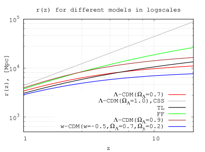
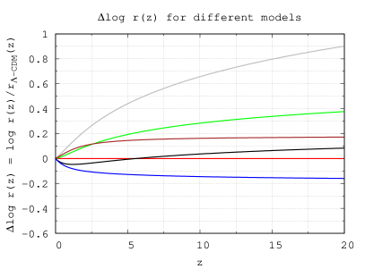
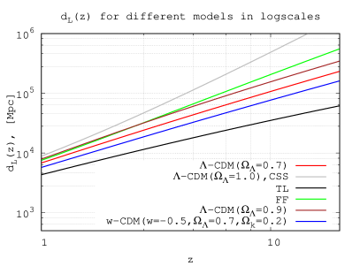
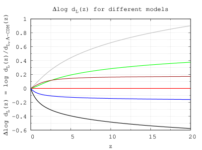
  Figure 7: The metric distance $r(z)$ (top) and the luminosity distance $d_{L}(z)$ (bottom) for six considered cosmological models described in Secs.2.2 and 2.3. Left: direct distances, Right: residuals from the standard $\Lambda$CDM model.

  Appendix C Hubble Diagram in logarithmic scale for considered cosmological models

  Figure 8 presents the HD in logarithmic scale and with the logarithmic scale median values ($\Delta\log{z}=0.1$) of the LGRB sample. The blue points are median values at $z<0.35$ and $4.2<z$, respectively. The points and curves are the same as in Fig.5.

  

  

  

  

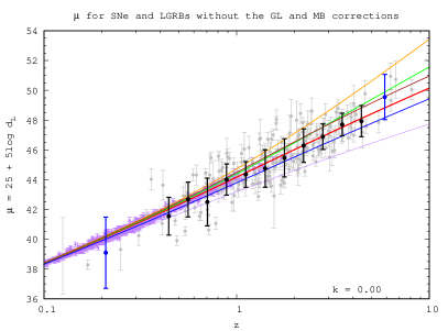
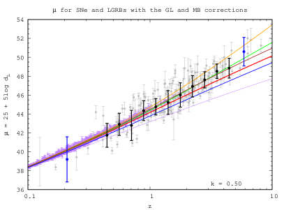
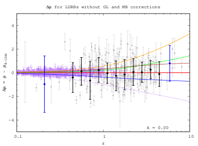
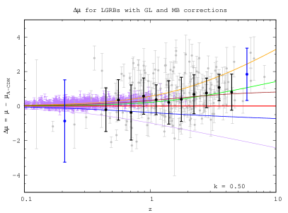
  Figure 8: Top panels: the luminosity distance modulus $\mu$ versus redshift (HD) in logarithmic $z$-scale for the SN Ia and LGRB samples. Black points are the median values of $\mu$ with logarithmic step $\Delta\log{z}=0.1$ of the LGRB sample. Bottom panels: the residuals $\Delta\mu$ from the standard $\Lambda$CDM model for the observed luminosity distance modulus. Left: without the correction for the GLB and MB. Right: corrected with $k=0.5$. The colour curves correspond to the cosmological models defined in Section 2.

References

- Acebron et al. (2020) Acebron A., et al., 2020, RELICS: A Very Large () Cluster Lens RXC J0032.1+1808, ApJ, in press, ApJ, arXiv:1912.02702
- Aghanim et al. (2018) Aghanim N., et al., 2018, Planck 2018 results. VI. Cosmological parameters, arXiv e-prints, arXiv:1807.06209
- Amati & Della Valle (2013) Amati L., Della Valle M., 2013, Measuring cosmological parameters with Gamma-Ray Bursts, Int. J. Modern Phys. D, 22, 1330028, arXiv:1310.3141
- Amati et al. (2002) Amati L., et al., 2002, Intrinsic spectra and energetics of BeppoSAX Gamma-Ray Bursts with known redshifts, A&A, 390, 81, astro-ph/0205230
- Amati et al. (2008) Amati L., Guidorzi C., Frontera F., Della Valle M., Finelli F., Landi R., Montanari E., 2008, Measuring the cosmological parameters with the correlation of gamma-ray bursts, MNRAS, 391, 577, arXiv:0805.0377
- Amati et al. (2018) Amati L., et al., 2018, The THESEUS space mission concept: science case, design and expected performances, Adv. Space Res., 62, 191
- Amati et al. (2019) Amati L., D’Agostino R., Luongo O., Muccino M., Tantalo M., 2019, Addressing the circularity problem in the correlation of Gamma-Ray Bursts, MNRAS, 486, L46
- Amendola et al. (2018) Amendola L., et al., 2018, Cosmology and fundamental physics with the Euclid satellite, Living Rev. Relativ., 21, 2, arXiv:1606.00180
- Band et al. (1993) Band D., et al., 1993, BATSE Observations of Gamma-Ray Burst Spectra. I. Spectral Diversity, ApJ, 413, 281
- Baryshev (2008) Baryshev Y. V., 2008, Field fractal cosmological model as an example of practical cosmology approach, in Baryshev Y. V., Taganov I. N., Teerikorpi P., eds, Problems of Practical Cosmology. Vol. 2. Russian Geographical Society, St. Petersburg, p. 60, arXiv:0810.0162
- Baryshev (2015) Baryshev Y. V., 2015, Paradoxes of cosmological physics in the beginning of the 21-st century, in Ryutin R. A., Petrov V. A., eds, Particle and Astroparticle Physics, Gravitation and Cosmology: Predictions, Observations and New Projects. World Scientific Press, Singapore, p. 297, arXiv:1501.01919
- Baryshev & Ezova (1997) Baryshev Y. V., Ezova Y. L., 1997, Gravitational mesolensing by King objects and quasar-galaxy associations, Astron. Rep., 74, 497
- Baryshev & Teerikorpi (2012) Baryshev Y., Teerikorpi P., 2012, Fundamental Questions of Practical Cosmology: Exploring the Realm of Galaxies. Springer-Verlag, Berlin
- Calvi et al. (2019) Calvi R., et al., 2019, MOS spectroscopy of protocluster candidate galaxies at , MNRAS, 489, 3294, arXiv:1908.01827
- Cano et al. (2017) Cano Z., Wang S.-Q., Dai Z.-G., Wu X.-F., 2017, The Observer’s Guide to the Gamma-Ray Burst Supernova Connection, Adv. Astron., 2017, 8929054, arXiv:1604.03549
- Castro-Tirado et al. (2018) Castro-Tirado A. J., Sokolov V. V., Guziy S. S., 2018, Gamma-ray bursts: Historical afterglows and early-time observations, in Sokolov V. V., Vlasuk V. V., Petkov V. B., eds, SN 1987A, Quark Phase Transition in Compact Objects and Multimessenger Astronomy. Moscow, p. 41
- Cervantes-Cota et al. (2020) Cervantes-Cota J. L., Galindo-Uribarri S., Smoot G. F., 2020, The Legacy of Einstein’s Eclipse, Gravitational Lensing, Universe, 6, 9, arXiv:1912.07674
- Clifton et al. (2012) Clifton T., Ferreira P. G., Padilla A., Skordis C., 2012, Modified Gravity and Cosmology, Phys. Rep., 513, 1, arXiv:1106.2476
- Courtois et al. (2013) Courtois H. M., Pomarède D., Tully R. B., Hoffman Y., Courtois D., 2013, Cosmography of the Local Universe, AJ, 146, 69, arXiv:1306.0091
- Dainotti et al. (2013a) Dainotti M. G., Cardone V. F., Piedipalumbo E., Capozziello S., 2013a, Slope evolution of GRB correlations and cosmology, MNRAS, 436, 82
- Dainotti et al. (2013b) Dainotti M. G., Petrosian V., Singal J., Ostrowski M., 2013b, Determination Of The Intrinsic Luminosity Time Correlation In The X-ray Afterglows Of Gamma-ray Bursts, ApJ, 774, 157
- De Rham et al. (2017) De Rham C., Deskins J. T., Tolley A. J., Zhou S.-Y., 2017, Graviton mass bounds, Rev. Mod. Phys., 89, 025004, arXiv:1606.08462
- Demianski et al. (2017a) Demianski M., Piedipalumbo E., Sawant D., Amati L., 2017a, Cosmology with gamma-ray bursts. I. The Hubble diagram through the calibrated correlation, A&A, 598, A112, arXiv:1610.00854
- Demianski et al. (2017b) Demianski M., Piedipalumbo E., Sawant D., Amati L., 2017b, Cosmology with gamma-ray bursts. II. Cosmography challenges and cosmological scenarios for the accelerated Universe, A&A, 598, A113, arXiv:1609.09631
- Deng et al. (2016) Deng C.-M., Wang X.-G., Guo B.-B., Lu R.-J., Wang Y.-Z., Wei J.-J., Wu X.-F., Liang E.-W., 2016, Cosmic Evolution of Long Gamma-Ray Burst Luminosity, ApJ, 820, 66, arXiv:1601.07645
- Einasto et al. (2016) Einasto M., et al., 2016, Sloan Great Wall as a complex of superclusters with collapsing cores, A&A, 595, A70, arXiv:1608.04988
- Francis et al. (2007) Francis M. J., Barnes L. A., James J. B., Lewis G. F., 2007, Expanding Space: the Root of all Evil?, Publ. Astron. Soc. Aust., 24, 95, astro-ph:0707.0380
- Gabrielli et al. (2005) Gabrielli A., Sylos Labini F., Joyce M., Pietronero L., 2005, Statistical Physics for Cosmic Structures. Springer-Verlag, Berlin
- Holz & Linder (2005) Holz D. E., Linder E. V., 2005, Safety in Numbers: Gravitational Lensing Degradation of the Luminosity Distance-Redshift Relation, ApJ, 631, 678, arXiv:astro-ph/0412173
- Holz & Wald (1998) Holz D. E., Wald R. M., 1998, New method for determining cumulative gravitational lensing effects in inhomogeneous universes, Phys. Rev. D, 58, 063501, arXiv:astro-ph/9708036
- Hoyle et al. (2000) Hoyle F., Burbidge G., Narlikar J. V., 2000, A Different Approach to Cosmology. Cambridge Univ. Press, Cambridge
- Hubble (1929) Hubble E., 1929, A relation between distance and radial velocity among extragalactic nebulae, Proc. Natl. Acad. Sci., 15, 168
- Ishak (2018) Ishak M., 2018, Testing general relativity in cosmology, Living Rev. Relativ., 22, 1, arXiv:1806.10122
- Ji et al. (2018) Ji L., Kovetz E. D., Kamionkowski M., 2018, Strong Lensing of Gamma Ray Bursts as a Probe of Compact Dark Matter, Phys. Rev. D, 98, 123523, arXiv:1809.09627
- Jönsson et al. (2008) Jönsson J., Kronborg T., Mortsell E., Sollerman J., 2008, Prospects and pitfalls of gravitational lensing in large supernova surveys, A&A, 487, 467, arXiv:0806.1387
- Jönsson et al. (2010) Jönsson et al., 2010, Constraining dark matter halo properties using lensed SNLS supernovae, MNRAS, 405, 535, arXiv:1002.1374
- Karachentsev et al. (2003) Karachentsev I., et al., 2003, Local galaxy flows within 5 Mpc, A&A, 398, 493, arXiv:astro-ph/0211011
- Kinugawa et al. (2019) Kinugawa T., Harikane Y., Asano K., 2019, Long gamma-ray burst rate at very high redshift, ApJ, 878, 128, arXiv:1901.03516
- Kodama et al. (2008) Kodama Y., Yonetoku D., Murakami T., Tanabe S., Tsutsui R., Nakamura T., 2008, Gamma-ray bursts in suggest that the time variation of the dark energy is small, MNRAS, 391, L1
- Kumar & Zhang (2015) Kumar P., Zhang B., 2015, The physics of gamma-ray bursts & relativistic jets, Phys. Rep., 561, 1, arXiv:1410.0679
- Kurt & Ougolnikov (2000) Kurt V. G., Ougolnikov O. S., 2000, A Search for Possible Mesolensing of Cosmic Gamma-Ray Bursts, Cosmic Res., 38, 213
- La Violette (1986) La Violette P. A., 1986, Is the Universe Really Expanding?, ApJ, 301, 544
- Laureijs et al. (2011) Laureijs et al., 2011, Euclid Definition Study Report, arXiv:1110.3193
- Liang et al. (2008) Liang N., Xiao W. K., Liu Y., Zhang S. N., 2008, A Cosmology-Independent Calibration of Gamma-Ray Burst Luminosity Relations and the Hubble Diagram, ApJ, 685, 354, arXiv:0802.4262
- Lietzen et al. (2016) Lietzen H., et al., 2016, Discovery of a massive supercluster system at , A&A, 588, L4, arXiv:1602.08498
- Lin et al. (2016a) Lin H.-N., Li X., Chang Z., 2016a, Model-independent distance calibration of high-redshift gamma-ray bursts and constrain on the CDM model, MNRAS, 455, 2131
- Lin et al. (2016b) Lin H.-N., Li X., Chang Z., 2016b, Effect of gamma-ray burst (GRB) spectra on the empirical luminosity correlations and the GRB Hubble diagram, MNRAS, 459, 2501
- Liu & Wei (2015) Liu J., Wei H., 2015, Cosmological models and gamma-ray bursts calibrated by using Padé method, Gen. Relativ. Gravitation, 47, 141, arXiv:1410.3960
- Lloyd-Ronning et al. (2019) Lloyd-Ronning N. M., Aykutalp A., Johnson J., 2019, On the Cosmological Evolution of Long Gamma-ray Burst Properties, MNRAS, 488, 5823, arXiv:1906.02278
- Lusso et al. (2019) Lusso E., Piedipalumbo E., Risaliti G., Paolillo M., Bisogni S., Nardini E., Amati L., 2019, Tension with the flat CDM model from a high redshift Hubble Diagram of supernovae, quasars and gamma-ray bursts, A&A, 628, L4, arXiv:1907.07692
- Meszaros & Rees (2014) Meszaros P., Rees M. J., 2014, Gamma-Ray Bursts, arXiv e-prints, arXiv:1401.3012
- Oguri & Takahashi (2006) Oguri M., Takahashi K., 2006, Gravitational lensing effects on the gamma-ray burst Hubble diagram, Phys. Rev. D, 73, 123002, arXiv:astro-ph/0604476
- Ougolnikov (2001) Ougolnikov O. S., 2001, The search for possible mesolensing of cosmic gamma-ray bursts. Double and triple bursts in BATSE catalogue, arXiv e-prints, arXiv:astro-ph/0111215
- Peacock (1999) Peacock J. A., 1999, Cosmological Physics. Cambridge Univ. Press, Cambridge
- Pearson & Hartley (1957) Pearson E. S., Hartley H. O., 1957, Biometrika Tables for Statisticians. Vol. 1, Cambridge Univ. Press, Cambridge
- Pe’er (2015) Pe’er A., 2015, Physics of Gamma-Ray Bursts Prompt Emission, Adv. Astron., 2015, 907321
- Perivolaropoulos & Kazantzidis (2019) Perivolaropoulos L., Kazantzidis L., 2019, Hints of Modified Gravity in Cosmos and in the Lab?, Int. J. Modern Phys. D, 28, 1942001, arXiv:1904.09462
- Perlmutter et al. (1999) Perlmutter S., et al., 1999, Measurements of Omega and Lambda from 42 high-redshift supernovae, ApJ, 517, 565, arXiv:astro-ph/9812133
- Riess et al. (1998) Riess A. G., et al., 1998, Observational evidence from supernovae for an accelerating universe and a cosmological constant, AJ, 116, 1009, arXiv:astro-ph/9805201
- Riess et al. (2019) Riess A. G., Casertano S., Yuan W., Macri L. M., Scolnic D., 2019, Large Magellanic Cloud Cepheid Standards Provide a 1 percent Foundation for the Determination of the Hubble Constant and Stronger Evidence for Physics beyond CDM and , ApJ, 876, 85, arXiv:1903.07603
- Sandage (1997) Sandage A., 1997, Astronomical problems for the next three decades, in Mamaso A., Munch G., eds, The Universe at Large: Key Issues in Astronomy and Cosmology. Cambridge Univ. Press, Cambridge, p. 1
- Sandage et al. (2010) Sandage A., Reindl B., Tammann G., 2010, The Linearity of the Cosmic Expansion Field from 300 to 30,000 km s-1 and the Bulk Motion of the Local Supercluster with Respect to the Cosmic Microwave Background, ApJ, 714, 1441, arXiv:0911.4925
- Schaefer (2007) Schaefer B., 2007, The Hubble Diagram to Redshift from 69 Gamma-Ray Bursts, ApJ, 660, 16, arXiv:astro-ph/0612285
- Scolnic et al. (2018) Scolnic D. M., et al., 2018, The Complete Light-curve Sample of Spectroscopically Confirmed SNe Ia from Pan-STARRS1 and Cosmological Constraints from the Combined Pantheon Sample, ApJ, 859, 101, arXiv:1710.00845
- Scolnic et al. (2019) Scolnic D. M., et al., 2019, The Next Generation of Cosmological Measurements with Type Ia Supernovae, Astro2020: Decadal Survey on Astronomy and Astrophysics. Science White Papers, No. 270, arXiv:1903.05128
- Shajib et al. (2020) Shajib A. J., et al., 2020, STRIDES: A 3.9 per cent measurement of the Hubble constant from the strong lens system DES J0408-354, MNRAS, 494, 6072, arXiv:1910.06306
- Shirokov et al. (2016) Shirokov S. I., Lovyagin N. Y., Baryshev Y. V., Gorokhov V. L., 2016, Large-Scale Fluctuations in the Number Density of Galaxies in Independent Surveys of Deep Fields, Astron. Rep., 60, 563, arXiv:1607.02596
- Smith et al. (2014) Smith M., et al., 2014, The Effect of Weak Lensing on Distance Estimates from Supernovae, ApJ, 780, 24, arXiv:1307.2566
- Sokolov et al. (2018a) Sokolov V. V., et al., 2018a, , in Sokolov V. V., Vlasuk V. V., Petkov V. B., eds, SN 1987A, Quark Phase Transition in Compact Objects and Multimessenger Astronomy. INR RAS, Moscow, p. 190
- Sokolov et al. (2018b) Sokolov I. V., Castro-Tirado A. J., Zhelenkova O. P., Solovyev I. A., Verkhodanov O. V., Sokolov V. V., 2018b, The Excess Density of Field Galaxies near around the Gamma-Ray Burst GRB021004 Position, Astroph. Bull., 73, 111, arXiv:1805.07082
- Strata et al. (2018) Strata G., et al., 2018, THESEUS: A key space mission concept for Multi-Messenger Astrophysics, Adv. Space Res., 62, 662, arXiv:1712.08153
- Tekhanovich & Baryshev (2016) Tekhanovich D. I., Baryshev Y. V., 2016, Global Structure of the Local Universe according to 2MRS Survey, Astrophys. Bull., 71, 155, arXiv:1610.05206
- Turner (2002) Turner M., 2002, Making Sense of the New Cosmology, Int. J. Modern Phys. A, 17, 180, arXiv:astro-ph/0202008
- Uzan (2003) Uzan J.-P., 2003, The fundamental constants and their variation: observational status and theoretical motivations, Rev. Mod. Phys., 75, 403, arXiv:hep-ph/0205340
- Valageas (2000) Valageas P., 2000, Statistical properties of the convergence due to weak gravitational lensing by non-linear structures, A&A, 356, 771, arXiv:astro-ph/9911336
- Wang & Dai (2011) Wang F. Y., Dai Z. G., 2011, Weak gravitational lensing effects on cosmological parameters and dark energy from gamma-ray bursts, A&A, 536, A96, arXiv:1112.4040
- Wang et al. (2002) Wang Y., Holz D. E., Munshi D., 2002, A Universal Probability Distribution Function for Weak-lensing Amplification, ApJ, 572, L15, arXiv:astro-ph/0204169
- Wang et al. (2011) Wang F.-Y., Qi S., Dai Z.-G., 2011, The updated luminosity correlations of gamma-ray bursts and cosmological implications, MNRAS, 415, 3423, arXiv:1105.0046
- Wang et al. (2016) Wang J. S., Wang F. Y., Cheng K. S., Dai Z. G., 2016, Measuring dark energy with the – correlation of gamma-ray bursts using model-independent methods, A&A, 585, A68, arXiv:1509.08558
- Wang et al. (2017) Wang G.-J., Yu H., Li Z.-X., Xia J.-Q., Zhu Z.-H., 2017, Evolutions and Calibrations of Long Gamma-Ray Bursts Luminosity Correlations Revisited, ApJ, 836, 103, arXiv: 1701.06102
- Wei & Wu (2017) Wei J.-J., Wu X.-F., 2017, Gamma-ray burst cosmology: Hubble diagram and star formation history, Int. J. Modern Phys. D, 26, arXiv:1607.01550
- Willingale & Mészáros (2017) Willingale R., Mészáros P., 2017, Gamma-Ray Bursts and Fast Transients. Multi-wavelength Observations and Multi-messenger Signals, Space Sci. Rev., 207, 63
- Woosley (1993) Woosley S. E., 1993, Gamma-ray bursts from stellar mass accretion disks around black holes, ApJ, 405, 273
- Woosley & Bloom (2006) Woosley S. E., Bloom J. S., 2006, The Supernova Gamma-Ray Burst Connection, ARA&A, 44, 507
- Xue et al. (2019) Xue L., Zhang F.-W., Zhu S.-Y., 2019, Characteristics of Long Gamma-Ray Bursts in the Comoving Frame, ApJ, 876, 77, arXiv:1904.07767
- Yonetoku et al. (2004) Yonetoku D., Murakami T., Nakamura T., Yamazaki R., Inoue A. K., Ioka K., 2004, Gamma-Ray Burst Formation Rate Inferred from the Spectral Peak Energy-Peak Luminosity Relation, ApJ, 609, 935