Theory and Algorithms for Shapelet-based Multiple-Instance Learning

Abstract

We propose a new formulation of Multiple-Instance Learning (MIL), in which a unit of data consists of a set of instances called a bag. The goal is to find a good classifier of bags based on the similarity with a “shapelet” (or pattern), where the similarity of a bag with a shapelet is the maximum similarity of instances in the bag. In previous work, some of the training instances are chosen as shapelets with no theoretical justification. In our formulation, we use all possible, and thus infinitely many shapelets, resulting in a richer class of classifiers. We show that the formulation is tractable, that is, it can be reduced through Linear Programming Boosting (LPBoost) to Difference of Convex (DC) programs of finite (actually polynomial) size. Our theoretical result also gives justification to the heuristics of some of the previous work. The time complexity of the proposed algorithm highly depends on the size of the set of all instances in the training sample. To apply to the data containing a large number of instances, we also propose a heuristic option of the algorithm without the loss of the theoretical guarantee. Our empirical study demonstrates that our algorithm uniformly works for Shapelet Learning tasks on time-series classification and various MIL tasks with comparable accuracy to the existing methods. Moreover, we show that the proposed heuristics allow us to achieve the result with reasonable computational time.

1 Introduction

Multiple-Instance Learning (MIL) is a fundamental framework of supervised learning with a wide range of applications such as prediction of molecular activity, and image classification. MIL has been extensively studied both in theoretical and practical aspects [14, 2, 26, 39, 13, 6], since the notion of MIL was first proposed by Dietterich et al. [11].

A standard MIL setting is described as follows: A learner receives sets $B_{1},B_{2},\ldots,B_{m}$ called bags; each contains multiple instances. In the training phase, each bag is labeled but instances are not labeled individually. The goal of the learner is to obtain a hypothesis that predicts the labels of unseen bags correctly. One of the most common hypotheses used in practice has the following form:

$$h_{\bf u}(B)=\max_{x\in B}\left\langle{\bf u},\Phi(x)\right\rangle,$$ (1)

where $\Phi$ is a feature map and ${\bf u}$ is a feature vector which we call a shapelet. In many applications, ${\bf u}$ is interpreted as a particular “pattern” in the feature space and the inner product as the similarity of $\Phi(x)$ from ${\bf u}$. Note that we use the term “shapelets” by following the terminology of Shapelet Learning (SL), which is a framework for time-series classification, although it is often called “concepts” in the literature of MIL. Intuitively, this hypothesis evaluates a given bag by the maximum similarity between the instances in the bag and the shapelet ${\bf u}$. Multiple-Instance Support Vector Machine (MI-SVM) proposed by Andrews et al. [2] is a widely used algorithm that employs this hypothesis class and learns ${\bf u}$. It is well-known that MIL algorithms using this hypothesis class perform empirically better in various multiple-instance datasets. Moreover, a generalization error bound of the hypothesis class is given by Sabato and Tishby [26].

However, in some domains such as image recognition and document classification, it is said that the hypothesis class (1) is not effective [see, e.g., 7]. To employ MIL on such domains more effectively, Chen et al. [7] extend a hypothesis to a convex combination of $h_{\bf u}$ :

$$g(B)=\sum_{{\bf u}\in U}w_{\bf u}\max_{x\in B}\left\langle{\bf u},\Phi(x)\right\rangle,$$ (2)

for some set $U$ of shapelets. In particular, Chen et al. consider $U_{\mathrm{train}}=\{\Phi(z)\mid z\in\bigcup_{i=1}^{m}B_{i}\}$, which is constructed from all instances in the training sample. The authors demonstrate that this hypothesis with the Gaussian kernel performs well in image recognition. The generalization bound provided by Sabato and Tishby [26] is applicable to a hypothesis class of the form (2) for the set $U$ of infinitely many shapelets ${\bf u}$ with bounded norm. Therefore, the generalization bound also holds for $U_{\mathrm{train}}$. However, it has never been theoretically discussed why such a fixed set $U_{\mathrm{train}}$ using training instances effectively works in MIL tasks.

1.1 Our Contributions

In this paper, we propose an MIL formulation with the hypothesis class (2) for sets $U$ of infinitely many shapelets.

The proposed learning framework is theoretically motivated and practically effective. We show the generalization error bound based on the Rademacher complexity [5] and large margin theory. The result indicates that we can achieve a small generalization error by keeping a large margin for large training sample.

The learning framework can be applied to various kinds of data and tasks because of our unified formulation. The existing shapelet-based methods are formulated for their target domains. More precisely, the existing shapelet-based methods are formulated using a fixed similarity measure (or distance), and the generalization ability is shown empirically in their target domains. For example, Chen et al. [7] and Sangnier et al. [27] calculated the feature vectors based on the similarity between every instance using the Gaussian kernel. In time-series domain, shapelet-based methods [35, 20, 17] usually use Euclidean distance as a similarity measure (or distance). By contrast, our framework employs a kernel function as a similarity measure. Therefore, our learning framework can be uniformly applied if we can set a kernel function as a similarity measure according to a target learning task. For example, the Gaussian kernel (behaves like the Euclidean distance) and Dynamic Time Warping (DTW) kernel [30]. Our framework can be also applied to non-real-valued sequence data (e.g., text, and a discrete signal) using a string kernel. Moreover, our generalization performance is guaranteed theoretically. The experimental results demonstrate that the provided approach uniformly works for SL and MIL tasks without introducing domain-specific parameters and heuristics, and compares with the state-of-the-art shapelet-based methods.

We show that the formulation is tractable. The algorithm is based on Linear Programming Boosting [LPBoost, 10] that solves the soft margin optimization problem via a column generation approach. Although the weak learning problem in the boosting becomes an optimization problem over an infinite-dimensional space, we can show that an analog of the representer theorem holds on it and allows us to reduce it to a non-convex optimization problem (difference of convex program) over a finite-dimensional space. While it is difficult to solve the sub-problems exactly because of non-convexity, it is possible to find good approximate solutions with reasonable time in many practical cases [see, e.g., 21].

Remarkably, our theoretical result gives justification to the heuristics of choosing the shapelets in the training instances. Our representer theorem indicates that at $t$-th iteration of boosting, the optimal solution ${\bf u}_{t}$ (i.e., shapelet) of the weak learning problem can be written as a linear combination of the feature maps of training instances, that is, ${\bf u}_{t}=\sum_{z\in\bigcup_{i=1}^{m}B_{i}}\alpha_{t,z}\Phi(z)$. Thus, we obtain a final classifier of the following form

$$g(B)=\sum_{t=1}^{T}w_{t}\max_{x\in B}\langle{\bf u}_{t},\Phi(x)\rangle=\sum_{t=1}^{T}w_{t}\max_{x\in B}\sum_{z\in\bigcup_{i=1}^{m}B_{i}}\alpha_{t,z}\langle\Phi(z),\Phi(x)\rangle.$$

Note that the hypothesis class used in the standard approach [7, 27] corresponds to the special case where ${\bf u}_{t}\in U_{\mathrm{train}}=\{\Phi(z)\mid z\in\bigcup_{i=1}^{m}B_{i}\}$. This observation would suggest that the standard approach of using $U_{\mathrm{train}}$ is reasonable.

1.2 Comparison to Related Work for MIL

There are many MIL algorithms with hypothesis classes which are different from (1) or (2). [e.g., 3, 14, 1, 38, 7]. For example, these algorithms adopted diverse approaches for the bag-labeling hypothesis from shapelet-based hypothesis classes (e.g., Zhang et al. [38] used a Noisy-OR based hypothesis and Gärtner et al. [14] proposed a new kernel called a set kernel). Shapelet-based hypothesis classes have a practical advantage of being applicable to SL in the time-series domain (see next subsection).

Sabato and Tishby [26] proved generalization bounds of hypotheses classes for MIL including those of (1) and (2) with infinitely large sets $U$. The generalization bound we provided in this paper is incomparable to the bound provided by Sabato and Tishby. When some data-dependent parameter is regarded as a constant, our bound is slightly better in terms of the sample size $m$ by the factor of $O(\log m)$. They also proved the PAC-learnability of the class (1) using the boosting approach under some technical assumptions. Their boosting approach is different from our work in that they assume that labels are consistent with some hypothesis of the form (1), while we consider arbitrary distributions over bags and labels.

1.3 Connection between MIL and Shapelet Learning for Time Series Classification

Here we mention briefly that MIL with type (2) hypotheses is closely related to SL, a framework for time-series classification that has been extensively studied [35, 20, 17, 15] in parallel to MIL. SL is a notion of learning with a feature extraction method, defined by a finite set $M\subseteq\mathbb{R}^{\ell}$ of real-valued “short” sequences called shapelets. A similarity measure is given by (not necessarily a Mercer kernel) $K:\mathbb{R}^{\ell}\times\mathbb{R}^{\ell}\to\mathbb{R}$ in the following way. A time series ${\boldsymbol{\tau}}=(\tau[1],\dots,\tau[L])\in\mathbb{R}^{L}$ can be identified with a bag $B_{\boldsymbol{\tau}}=\{(\tau[j],\ldots,\tau[j+\ell-1])\mid 1\leq j\leq L-\ell+1\}$ consisting of all subsequences of ${\boldsymbol{\tau}}$ of length $\ell$. The feature of ${\boldsymbol{\tau}}$ is a vector $\left(\max_{{\bf x}\in B_{\boldsymbol{\tau}}}K({\bf z},{\bf x})\right)_{{\bf z}\in M}$ of a fixed dimension $|M|$ regardless of the length $L$ of the time series ${\boldsymbol{\tau}}$. When we employ a linear classifier on top of the features, we obtain a hypothesis in the form:

$$g({\boldsymbol{\tau}})=\sum_{{\bf z}\in M}w_{\bf z}\max_{{\bf x}\in B_{\tau}}K({\bf z},{\bf x}),$$ (3)

which is essentially the same form as (2), except that finding good shapelets $M$ is a part of the learning task, as well as to find a good weight vector ${\bf w}$. This task is one of the most successful approaches for SL [17, 15, 16, 25, 18], where a typical choice of $K$ is $K({\bf z},{\bf x})=-\|{\bf z}-{\bf x}\|_{2}$. However, almost all existing methods heuristically choose shapelets $M$ and with no theoretical guarantee on how good the choice of $M$ is.

Note also that in the SL framework, each ${\bf z}\in M$ is called a shapelet, while in this paper, we assume that $K$ is a kernel $K(z,x)=\langle\Phi(z),\Phi(x)\rangle$ and any ${\bf u}$ (not necessarily $\Phi(z)$ for some $z$) in the Hilbert space is called a shapelet.

Sangnier et al. [27] proposed an MIL-based anomaly detection algorithm for time series data. They showed an algorithm based on LPBoost and the generalization error bound based on the Rademacher complexity [5]. Their hypothesis class is same as [7]. However, they did not analyze the theoretical justification to use finite set $U$ made from training instances (the authors mentioned as future work). By contrast, we consider a hypothesis class based on infinitely many shapelets, and our representer theorem guarantees that our learning problem over the infinitely large set is still tractable. As a result, our study justifies the previous heuristics of their approach.

There is another work which treats shapelets not appearing in the training set. Learning Time-Series Shapelets (LTS) algorithm [15] tries to solve a non-convex optimization problem of learning effective shapelets in an infinitely large domain. However, there is no theoretical guarantee of its generalization error. In fact, our generalization error bound applies to their hypothesis class.

For SL tasks, many researchers focus on improving efficiency [20, 25, 16, 34, 18, 19]. However, these methods are specialized in the time-series domain, and the generalization performance has never been theoretically discussed.

Curiously, despite MIL and SL share similar motivations and hypotheses, the relationship between MIL and SL has not yet been pointed out. From the shapelet-perspective in MIL, the hypothesis (1) is regarded as a “single shapelet”-based hypothesis, and the hypothesis (2) is regarded as a “multiple-shapelets”-based hypothesis. In this study, we refer to a linear combination of maximum similarities based on shapelets such as (2) and (3) as shapelet-based classifiers.

2 Preliminaries

Let ${\mathcal{X}}$ be an instance space. A bag $B$ is a finite set of instances chosen from ${\mathcal{X}}$. The learner receives a sequence of labeled bags $S=((B_{1},y_{1}),\ldots,(B_{m},y_{m}))\in(2^{{\mathcal{X}}}\times\{-1,1\})^{m}$ called a sample, where each labeled bag is independently drawn according to some unknown distribution $D$ over $2^{{\mathcal{X}}}\times\{-1,1\}$. Let ${P_{S}}$ denote the set of all instances that appear in the sample $S$. That is, ${P_{S}}=\bigcup_{i=1}^{m}B_{i}$. Let $K$ be a kernel over ${\mathcal{X}}$, which is used to measure the similarity between instances, and let $\Phi:{\mathcal{X}}\to{\mathbb{H}}$ denote a feature map associated with the kernel $K$ for a Hilbert space ${\mathbb{H}}$, that is, $K(z,z^{\prime})=\langle\Phi(z),\Phi(z^{\prime})\rangle$ for instances $z,z^{\prime}\in{\mathcal{X}}$, where $\langle\cdot,\cdot\rangle$ denotes the inner product over ${\mathbb{H}}$. The norm induced by the inner product is denoted by $\|\cdot\|_{\mathbb{H}}$ defined as $\|{\bf u}\|_{{\mathbb{H}}}=\sqrt{\langle{\bf u},{\bf u}\rangle}$ for ${\bf u}\in{\mathbb{H}}$.

For each ${\bf u}\in{\mathbb{H}}$ which we call a shapelet, we define a shapelet-based classifier denoted by $h_{{\bf u}}$, as the function that maps a given bag $B$ to the maximum of the similarity scores between shapelet ${\bf u}$ and $\Phi(x)$ over all instances $x$ in $B$. More specifically,

$$h_{{\bf u}}(B)=\max_{x\in B}\left\langle{\bf u},\Phi(x)\right\rangle.$$

For a set $U\subseteq{\mathbb{H}}$, we define the class of shapelet-based classifiers as

$$H_{U}=\left\{h_{{\bf u}}\mid{\bf u}\in U\right\}$$

and let ${\mathrm{conv}}(H_{U})$ denote the set of convex combinations of shapelet-based classifiers in $H_{U}$. More precisely,

$${\mathrm{conv}}(H_{U})= \left\{\int_{{\bf u}\in U}w_{\bf u}h_{\bf u}d{\bf u}\mid\text{$w_{\bf u}$ is a density over $U$}\right\}$$

$$= \left\{\sum_{{\bf u}\in U^{\prime}}w_{\bf u}h_{\bf u}\mid\forall{\bf u}\in U^{\prime},w_{\bf u}\geq 0,\right.$$

$$\left.\sum_{{\bf u}\in U^{\prime}}w_{\bf u}=1,\text{$U^{\prime}\subseteq U$ is a finite support}\right\}.$$ (4)

The goal of the learner is to find a hypothesis $g\in{\mathrm{conv}}(H_{U})$, so that its generalization error ${\mathcal{E}}_{D}(g)=\Pr_{(B,y)\sim D}[{\mathrm{sign}}(g(B))\neq y]$ is small. Note that since the final hypothesis ${\mathrm{sign}}\circ g$ is invariant to any scaling of $g$, we assume without loss of generality that

$$U=\{{\bf u}\in{\mathbb{H}}\mid\|{\bf u}\|_{\mathbb{H}}\leq 1\}.$$

Let ${\mathcal{E}}_{\rho}(g)$ denote the empirical margin loss of $g$ over $S$, that is, ${\mathcal{E}}_{\rho}(g)=|\{i\mid y_{i}g(B_{i})<\rho\}|/m$.

3 Optimization Problem Formulation

In this paper, we formulate the problem as soft margin maximization with $1$-norm regularization, which ensures a generalization bound for the final hypothesis [see, e.g., 10]. Specifically, the problem is formulated as a linear programming problem (over infinitely many variables) as follows:

$$\max\limits_{\rho,w,{\bf\xi}}\; \rho-\frac{1}{\nu m}\sum_{i=1}^{m}\xi_{i}$$ (5)

sub.to $$\int_{{\bf u}\in U}y_{i}w_{{\bf u}}h_{\bf u}(B_{i})d{\bf u}\geq\rho-\xi_{i}\wedge\xi_{i}\geq 0,~{}i\in[m],$$

$$\int_{{\bf u}\in U}w_{{\bf u}}d{\bf u}=1,w_{\bf u}\geq 0,~{}\rho\in\mathbb{R},$$

where $\nu\in[0,1]$ is a parameter. To avoid the integral over the Hilbert space, it is convenient to consider the dual form:

$$\min\limits_{\gamma,{\bf d}}\; \gamma$$ (6)

sub.to $$\sum_{i=1}^{m}y_{i}d_{i}h_{\bf u}(B_{i})\leq\gamma,\;{\bf u}\in U,$$

$$0\leq d_{i}\leq 1/(\nu m),\;i\in[m],$$

$$\sum_{i=1}^{m}d_{i}=1,~{}\gamma\in\mathbb{R}.$$

The dual problem is categorized as a semi-infinite program because it contains infinitely many constraints. Note that the duality gap is zero because the problem (6) is linear and the optimum is finite [see Theorem 2.2 of 29]. We employ column generation to solve the dual problem: solve (6) for a finite subset $U^{\prime}\subseteq U$, find ${\bf u}$ to which the corresponding constraint is maximally violated by the current solution (column generation part), and repeat the procedure with $U^{\prime}=U^{\prime}\cup\{{\bf u}\}$ until a certain stopping criterion is met. In particular, we use LPBoost [10], a well-known and practically fast algorithm of column generation. Since the solution ${\bf w}$ is expected to be sparse due to the 1-norm regularization, the number of iterations is expected to be small.

Following the boosting terminology, we refer to the column generation part as weak learning. In our case, weak learning is formulated following the optimization problem:

$$\max_{{\bf u}\in{\mathbb{H}}}\;\sum_{i=1}^{m}y_{i}d_{i}\max_{x\in B_{i}}\left\langle{\bf u},\Phi\left(x\right)\right\rangle\;\text{sub.to}\;\|{\bf u}\|_{\mathbb{H}}^{2}\leq 1.$$ (7)

Thus, we need to design a weak learner for solving (7) for a given sample weighted by ${\bf d}$. However, it seems to be impossible to solve it directly because we only have access to $U$ through the associated kernel. Fortunately, we prove a version of representer theorem given below, which makes (7) tractable.

Theorem 1 (Representer Theorem)

The solution ${\bf u}^{*}$ of (7) can be written as ${\bf u}^{*}=\sum_{z\in{P_{S}}}\alpha_{z}\Phi(z)$ for some real numbers $\alpha_{z}$.

Our theorem can be derived from a non-trivial application of the standard representer theorem [see, e.g., 23]. Intuitively, we prove the theorem by decomposing the optimization problem (7) into a number of sub-problems, so that the standard representer theorem can be applied to each of the sub-problems. The detail of the proof is given in Appendix A.

This result gives justification to the simple heuristics in the standard approach: choosing the shapelets based on the training instances. More precisely, the hypothesis class used in the standard approach [7, 27] corresponds to the special case where ${\bf u}\in U_{\mathrm{train}}=\{\Phi(z)\mid z\in P_{S}\}$. Thus, our representer theorem would suggest that the standard approach of using $U_{\mathrm{train}}$ is reasonable.

Theorem 1 says that the weak learning problem can be rewritten in the following tractable form:

OP 1

Weak Learning Problem

$$\min_{{\boldsymbol{\alpha}}}\; -\sum_{i=1}^{m}{d}_{i}y_{i}\max_{x\in B_{i}}\sum_{z\in{P_{S}}}\alpha_{z}K\left(z,x\right)$$

$$\mathrm{sub.to}\; \sum_{z\in{P_{S}}}\sum_{v\in{P_{S}}}\alpha_{z}\alpha_{v}K\left(z,v\right)\leq 1.$$

Unlike the primal solution ${\bf w}$, the dual solution ${\boldsymbol{\alpha}}$ is not expected to be sparse. To obtain a more interpretable hypothesis, we propose another formulation of weak learning where 1-norm regularization is imposed on ${\boldsymbol{\alpha}}$, so that a sparse solution of ${\boldsymbol{\alpha}}$ will be obtained. In other words, instead of $U$, we consider the feasible set $\hat{U}=\left\{\sum_{z\in{P_{S}}}\alpha_{z}\Phi(z):\|{\boldsymbol{\alpha}}\|_{1}\leq 1\right\}$, where $\|{\boldsymbol{\alpha}}\|_{1}$ is the 1-norm of ${\boldsymbol{\alpha}}$.

OP 2

Sparse Weak Learning Problem

$$\min_{{\boldsymbol{\alpha}}}\; -\sum_{i=1}^{m}{d}_{i}y_{i}\max_{x\in B_{i}}\sum_{z\in{P_{S}}}\alpha_{z}K\left(z,x\right)$$

$$\mathrm{sub.to}\;\; \|{\boldsymbol{\alpha}}\|_{1}\leq 1$$

Note that when running LPBoost with a weak learner for OP 2, we obtain a final hypothesis that has the same form of generalization bound as the one stated in Theorem 2, which is of a final hypothesis obtained when used with a weak learner for OP 1. To see this, consider a feasible space $\hat{U}_{\Lambda}=\left\{\sum_{z\in{P_{S}}}\alpha_{z}\Phi(z):\|{\boldsymbol{\alpha}}\|_{1}\leq\Lambda\right\}$ for a sufficiently small $\Lambda>0$, so that $\hat{U}_{\Lambda}\subseteq U$. Then since $H_{\hat{U}_{\Lambda}}\subseteq H_{U}$, a generalization bound for $H_{U}$ also applies to $H_{\hat{U}_{\Lambda}}$. On the other hand, since the final hypothesis ${\mathrm{sign}}\circ g$ for $g\in{\mathrm{conv}}(H_{\hat{U}_{\Lambda}})$ is invariant to the scaling factor $\Lambda$, the generalization ability is independent of $\Lambda$.

4 Algorithms

In this section, we present the pseudo-code of LPBoost in Algorithm 1 for completeness. Moreover, we describe our algorithms for the weak learners. For simplicity, we denote by ${\mathbf{k}}_{x}\in\mathbb{R}^{P_{S}}$ a vector given by $k_{x,z}=K(z,x)$ for every $z\in P_{S}$. The objective function of OP 1 (and OP 2) is rewritten as

$$\sum_{i:y_{i}=-1}d_{i}\max_{x\in B_{i}}{\mathbf{k}}_{x}^{T}{\boldsymbol{\alpha}}-\sum_{i:y_{i}=1}d_{i}\max_{x\in B_{i}}{\mathbf{k}}_{x}^{T}{\boldsymbol{\alpha}},$$

which can be seen as a difference $F-G$ of two convex functions $F$ and $G$ of ${\boldsymbol{\alpha}}$. Therefore, the weak learning problems are DC programs and thus we can use DC algorithm [31, 36] to find an $\epsilon$-approximation of a local optimum. We employ a standard DC algorithm. That is, for each iteration $t$, we linearize the concave term $G$ with $\nabla_{{\boldsymbol{\alpha}}}G({\boldsymbol{\alpha}}_{t})^{T}{\boldsymbol{\alpha}}$ at the current solution ${\boldsymbol{\alpha}}_{t}$, which is $\sum_{i:y_{i}=1}d_{i}{\mathbf{k}}_{x_{i}^{*}}^{T}{\boldsymbol{\alpha}}$ with $x_{i}^{*}=\arg\max_{x\in B_{i}}{\mathbf{k}}_{x}^{T}{\boldsymbol{\alpha}}$ in our case, and then update the solution to ${\boldsymbol{\alpha}}_{t+1}$ by solving the resultant convex optimization problem $\textsf{OP}^{\prime}_{t}$.

In addition, the problems $\textsf{OP}^{\prime}_{t}$ for OP 1 and OP 2 are reformulated as a second-order cone programming (SOCP) problem and an LP problem, respectively, and thus both problems can be efficiently solved. To this end, we introduce new variables $\lambda_{i}$ for all negative bags $B_{i}$ with $y_{i}=-1$ which represent the factors $\max_{x\in B_{i}}{\mathbf{k}}_{x}^{T}{\boldsymbol{\alpha}}$. Then we obtain the equivalent problem to $\textsf{OP}^{\prime}_{t}$ for OP 1 as follows:

$$\min_{{\boldsymbol{\alpha}},{\boldsymbol{\lambda}}}\; \sum_{i:y_{i}=-1}d_{i}\lambda_{i}-\sum_{i:y_{i}=1}d_{i}\max_{x\in B_{i}}{\mathbf{k}}_{x}^{T}{\boldsymbol{\alpha}}$$ (8)

sub.to $${\mathbf{k}}_{x}^{T}{\boldsymbol{\alpha}}\leq\lambda_{i}~{}(\forall i:y_{i}=-1,\forall x\in B_{i}),$$

$$\sum_{z\in{P_{S}}}\sum_{v\in{P_{S}}}\alpha_{z}\alpha_{v}K\left(z,v\right)\leq 1.$$

It is well known that this is an SOCP problem. Moreover, it is clear that $\textsf{OP}^{\prime}_{t}$ for OP 2 can be formulated as an LP problem. We describe the algorithm for OP 1 in Algorithm 2.

One may concern that a kernel matrix may become large when a sample consists a large amount of bags and instances. However, note that the kernel matrix of $K(z,x)$ which is used in Algorithm 2 needs to be computed only once at the beginning of Algorithm 1, not at every iteration.

As a result, our learning algorithm outputs a classifier

$$g(B)=\mathrm{sign}\left(\sum_{t=1}^{T}{w_{t}}\max_{x\in B}\sum_{z\in P_{S}}\alpha_{t,z}K(z,x)\right)$$

where $w_{t}$ and ${\boldsymbol{\alpha}}_{t}$ are obtained in training phase. Therefore, the computational cost for predicting the label of $B$ is $O(T|P_{S}||B|)$ in the worst case when all elements of $\alpha_{t,z}$ are non-zero. However, when we employ our sparse formulation OP 2 which allows us to find a sparse $\alpha$, the computational cost is expected to be much smaller than the worst case.

Algorithm 1 LPBoost using WeakLearn

Inputs:

      $S$, kernel $K$, $\nu\in(0,1]$, $\epsilon>0$

Initialize:

      ${\bf d}_{0}\leftarrow(\frac{1}{m},\ldots,\frac{1}{m}),\gamma=0$

for  $t=1,\dots$ do

     $h_{t}\leftarrow$ Run WeakLearn($S$, $K$, ${\bf d}_{t-1}$, $\epsilon$)

     if $\sum_{i=1}^{m}y_{i}d_{i}h_{t}(B_{i})\leq\gamma$ then

         $t=t-1$, break

     end if

      $\displaystyle(\gamma,{\bf d}_{t})\leftarrow\arg\min\limits_{\gamma,{\bf d}}\;\gamma$ $\displaystyle\text{sub.to}~{}~{}\sum_{i=1}^{m}y_{i}d_{i}h_{j}(B_{i})\leq\gamma~{}~{}(j=1,\ldots,t),~{}~{}$ $\displaystyle 0\leq d_{i}\leq 1/\nu m~{}~{}(i\in[m]),\sum_{i=1}^{m}d_{i}=1,~{}\gamma\in\mathbb{R}.$

end for

${\bf w}\leftarrow$ Lagrangian multipliers of the last solution

$g\leftarrow\sum_{j=1}^{t}w_{j}h_{j}$

return ${\mathrm{sign}}(g)$

Algorithm 2 WeakLearn using the DC Algorithm

Inputs:

      $S$, $K$, ${\bf d}$, $\epsilon$ (convergence parameter)

Initialize:

      ${\boldsymbol{\alpha}}_{0}\in\mathbb{R}^{|{P_{S}}|}$, $f_{0}\leftarrow\infty$

for $t=1,\dots$ do

     for $\forall k:y_{k}=+1$ do

         $\displaystyle x^{*}_{k}\leftarrow\arg\max_{x\in B_{k}}\sum_{z\in{P_{S}}}d_{k}\alpha_{t,z}K\left(z,x\right)$

     end for

      $\displaystyle f\leftarrow\min_{{\boldsymbol{\alpha}},\boldsymbol{\lambda}}\;$ $\displaystyle-\sum_{k:y_{k}=+1}{d}_{k}\sum_{z\in{P_{S}}}\alpha_{z}K\left(z,x_{k}^{*}\right)+\sum_{r:y_{r}=-1}{d}_{r}\lambda_{r}$ (9) sub.to $\displaystyle\sum_{z\in{P_{S}}}\alpha_{z}K\left(z,x\right)\leq\lambda_{r}~{}(\forall r:y_{r}=-1,\forall x\in B_{r}),$ $\displaystyle\sum_{z\in{P_{S}}}\sum_{v\in{P_{S}}}\alpha_{z}\alpha_{v}K\left(z,v\right)\leq 1.$

     ${\boldsymbol{\alpha}}_{t}\leftarrow{\boldsymbol{\alpha}}$, $f_{t}\leftarrow f$

     if $f_{t-1}-f_{t}\leq\epsilon$ then

         break

     end if

end for

return $h(B)=\max_{x\in B}\sum_{z\in{P_{S}}}\alpha_{t,z}K(z,x)$

5 Generalization Bound of the Hypothesis Class

In this section, we provide a generalization bound of hypothesis classes ${\mathrm{conv}}(H_{U})$ for various $U$ and $K$.

Let $\Phi(P_{S})=\{\Phi(z)\mid z\in P_{S}\}$. Let ${\Phi_{\mathrm{diff}}(P_{S})}=\{\Phi(z)-\Phi(z^{\prime})\mid z,z^{\prime}\in P_{S},z\neq z^{\prime}\}$. By viewing each instance ${{\bf v}}\in{\Phi_{\mathrm{diff}}(P_{S})}$ as a hyperplane $\{{\bf u}\mid\langle{{\bf v}},{\bf u}\rangle=0\}$, we can naturally define a partition of the Hilbert space ${\mathbb{H}}$ by the set of all hyperplanes ${{\bf v}}\in{\Phi_{\mathrm{diff}}(P_{S})}$. Let ${\mathcal{I}}$ be the set of all cells of the partition, that is, ${\mathcal{I}}=\{I\mid I=\cap_{{{\bf v}}\in V}\{{\bf u}\mid\langle{{\bf v}},{\bf u}\rangle>0\},I\neq\emptyset,V\subseteq\Phi_{\mathrm{diff}}(P_{S}),{\bf v}\in V\Leftrightarrow-{\bf v}\notin V\mathrm{~{}for~{}all~{}}{\bf v}\in\Phi_{\mathrm{diff}}(P_{S})\}$. Each cell $I\in{\mathcal{I}}$ is a polyhedron which is defined by a minimal set $V_{I}\subseteq{\Phi_{\mathrm{diff}}(P_{S})}$ that satisfies $I=\bigcap_{{{\bf v}}\in V_{I}}\{{\bf u}\mid\langle{\bf u},{{\bf v}}\rangle>0\}$. Let

$$\mu^{*}=\min_{I\in{\mathcal{I}}}\max_{{\bf u}\in I\cap U}\min_{{{\bf v}}\in V_{I}}|\langle{\bf u},{{\bf v}}\rangle|.$$

Let $d^{*}_{\Phi,S}$ be the VC dimension of the set of linear classifiers over the finite set ${\Phi_{\mathrm{diff}}(P_{S})}$, given by $F_{U}=\{f:{{\bf v}}\mapsto{\mathrm{sign}}(\langle{\bf u},{{\bf v}}\rangle)\mid{\bf u}\in U\}$.

Then we have the following generalization bound on the hypothesis class of (2).

Theorem 2

Let $\Phi:{\mathcal{X}}\rightarrow{\mathbb{H}}$. Suppose that for any $z\in{\mathcal{X}}$, $\|\Phi(z)\|_{\mathbb{H}}\leq R$. Then, for any $\rho>0$, with high probability the following holds for any $g\in{\mathrm{conv}}(H_{U})$ with $U\subseteq\{{\bf u}\in{\mathbb{H}}\mid\|{\bf u}\|_{\mathbb{H}}\leq 1\}$:

$${\mathcal{E}}_{D}(g)\leq {\mathcal{E}}_{\rho}(g)+O\left(\frac{R\sqrt{d_{\Phi,S}^{*}\log|{P_{S}}|}}{\rho\sqrt{m}}\right),$$ (10)

where (i) for any $\Phi$, $d^{*}_{\Phi,S}=O((R/\mu^{*})^{2})$, (ii) if ${\mathcal{X}}\subseteq\mathbb{R}^{\ell}$ and $\Phi$ is the identity mapping (i.e., the associated kernel is the linear kernel), or (iii) if ${\mathcal{X}}\subseteq\mathbb{R}^{\ell}$ and $\Phi$ satisfies the condition that $\left\langle\Phi(z),\Phi(x)\right\rangle$ is monotone decreasing with respect to $\|z-x\|_{2}$ (e.g., the mapping defined by the Gaussian kernel) and $U=\{\Phi(z)\mid z\in\mathbb{R}^{\ell},\|\Phi(z)\|_{\mathbb{H}}\leq 1\}$, then $d^{*}_{\Phi,S}=O(\min((R/\mu^{*})^{2},\ell))$.

We show the proof in Appendix B.

Comparison with the existing bounds

A similar generalization bound can be derived from a known bound of the Rademacher complexity of $H_{U}$ [Theorem 20 of 26] and a generalization bound of ${\mathrm{conv}(H)}$ for any hypothesis class $H$ [see Corollary 6.1 of 23]:

$${\mathcal{E}}_{D}(g)\leq{\mathcal{E}}_{\rho}(g)+O\left(\frac{{\log\left(\sum_{i=1}^{m}|B_{i}|\right)\log(m)}}{\rho\sqrt{m}}\right).$$

Note that Sabato and Tishby [26] fixed $R=1$. For simplicity, we omit some constants of [Theorem 20 of 26]. Note that $|{P_{S}}|\leq\sum_{i=1}^{m}|B_{i}|$ by definition. The bound above is incomparable to Theorem 2 in general, as ours uses the parameter $d^{*}_{\Phi,S}$ and the other has the extra $\sqrt{\log\left(\sum_{i=1}^{m}|B_{i}|\right)}\log(m)$ term. However, our bound is better in terms of the sample size $m$ by the factor of $O(\log m)$ when other parameters are regarded as constants.

6 SL by MIL

6.1 Time-Series Classification with Shapelets

In the following, we introduce a framework of time-series classification problem based on shapelets (i.e., SL problem). As mentioned in the previous section, a time series ${\boldsymbol{\tau}}=(\tau[1],\dots,\tau[L])\in\mathbb{R}^{L}$ can be identified with a bag $B_{\boldsymbol{\tau}}=\{(\tau[j],\ldots,\tau[j+\ell-1])\mid 1\leq j\leq L-\ell+1\}$ that consists of all subsequences of ${\boldsymbol{\tau}}$ of length $\ell$. The learner receives a labeled sample $S=((B_{{\boldsymbol{\tau}}_{1}},y_{1}),\ldots,(B_{{\boldsymbol{\tau}}_{m}},y_{m}))\in(2^{\mathbb{R}{{}^{\ell}}}\times\{-1,1\})^{m}$, where each labeled bag (i.e. labeled time series) is independently drawn according to some unknown distribution $D$ over a finite support of $2^{\mathbb{R}^{\ell}}\times\{-1,+1\}$. The goal of the learner is to predict the labels of an unseen time series correctly. In this way, the SL problem can be viewed as an MIL problem, and thus we can apply our algorithms and theory.

Note that, for time-series classification, various similarity measures can be represented by a kernel. For example, the Gaussian kernel (behaves like the Euclidean distance) and Dynamic Time Warping (DTW) kernel. Moreover, our framework can generally apply to non-real-valued sequence data (e.g., text, and a discrete signal) using a string kernel.

6.2 Our Theory and Algorithms for SL

By Theorem 2, we can immediately obtain the generalization bound of our hypothesis class in SL as follows:

Corollary 3

Consider time-series sample $S$ of size $m$ and length $L$. For any fixed $\ell<L$, the following generalization error bound holds for all $g\in{\mathrm{conv}}(H_{U})$ in which the length of shapelet is $\ell$:

$${\mathcal{E}}_{D}(g)\leq{\mathcal{E}}_{\rho}(g)+O\left(\frac{R\sqrt{d_{\Phi,S}^{*}\log(m(L-\ell+1))}}{\rho\sqrt{m}}\right).$$

To the best of our knowledge, this is the first result on the generalization performance of SL.

Theorem 1 gives justification to the heuristics which choose the shapelets extracted from the instances appearing in the training sample (i.e., the subsequences for SL tasks). Moreover, several methods using a linear combination of shapelet-based classifiers [e.g., 17, 15], are supported by Corollary 3.

For time-series classification problem, shapelet-based classification has a greater advantage of the interpretability or visibility than other time-series classification methods [see, e.g., 35]. Although we use a nonlinear kernel function, we can observe important subsequences that contribute to effective shapelets by solving OP 2 because of the sparsity (see also the experimental results). Moreover, for unseen time-series data, we can observe the type of subsequences that contribute to the predicted class by observing maximizer $x\in B$.

6.3 Learning Shapelets of Different Lengths

For time-series classification, many existing methods take advantage of using shapelets of various lengths. Below, we show that our formulation can be easily applied to the case.

A time series ${\boldsymbol{\tau}}=(\tau[1],\dots,\tau[L])\in\mathbb{R}^{L}$ can be identified with a bag $B_{\boldsymbol{\tau}}=\{(\tau[j],\ldots,\tau[j+\ell-1])\mid 1\leq j\leq L-\ell+1,\forall\ell\in Q\}$ that consists of all length $\ell\in Q\subseteq\{1,\ldots,L\}$ of subsequences of ${\boldsymbol{\tau}}$. That is, this is also a special case of MIL that a bag contains different dimensional instances.

There is a simple way to apply our learning algorithm to this case. We just employ some kernels $K(z,x)$ which supports different dimensional instance pairs $z$ and $x$. Fortunately, such kernels have been studied well in the time-series domain. For example, DTW kernel and Global Alignment kernel [9] are well-known kernels which support time series of different lengths. However, the size of the kernel matrix of $K(z,x)$ becomes $m(\sum_{\ell\in Q}(L-\ell+1))^{2}$. In practice, it requires high memory cost for large time-series data. Moreover, in general, the above kernel requires a higher computational cost than standard kernels.

We introduce a practical way to learn shapelets of different lengths based on heuristics. In each weak learning problem, we decomposed the original weak learning problem over different dimensional data space into the weak learning problems over each dimensional data space. For example, we consider solving the following problem instead of the weak learning problem OP 1:

$$\min_{\ell}\min_{{\boldsymbol{\alpha}}}\; -\sum_{i=1}^{m}{d}_{i}y_{i}\max_{x\in B_{i}^{\ell}}\sum_{z\in{P_{S}}^{\ell}}\alpha_{z}K\left(z,x\right),$$

sub.to $$\sum_{z\in{P_{S}}^{\ell}}\sum_{v\in{P_{S}}^{\ell}}\alpha_{z}\alpha_{v}K\left(z,v\right)\leq 1.$$

where $B_{i}^{\ell}$ denotes the $\ell$ dimensional instances (i.e., length $\ell$ of subsequences) in $B_{i}$, and ${P_{S}}^{\ell}$ denotes $\bigcup_{i=1}^{m}B_{i}^{\ell}$. The total size of kernel matrices becomes $m\sum_{\ell\in Q}((L-\ell+1))^{2}$, and thus this method does not require so large kernel matrix. Moreover, in this way, we do not need to use a kernel which supports different dimensional instances. Note that, even using this heuristic, the obtained final hypothesis has theoretical generalization performance. This is because the hypothesis class still represented as the form of (2). In our experiment, we use the latter method by giving weight to memory efficiency.

6.4 Heuristics for computational efficiency

For the practical applications, we introduce some heuristics for improving efficiency in our algorithm.

Reduction of ${P_{S}}$

Especially for time-series data, the size $|{P_{S}}|$ often becomes large because $|{P_{S}}|=O(mL)$. Therefore, constructing a kernel matrix of $|{P_{S}}|\times|{P_{S}}|$ has high computational costs for time-series data. For example, when we consider subsequences as instances for time series classification, we have a large computational cost because of the number of subsequences of training data (e.g., approximately $10^{6}$ when sample size is $1000$ and length of each time series is $1000$, which results in a similarity matrix of size $10^{12}$). However, in most cases, many subsequences in time series data are similar to each other. Therefore, we only use representative instances ${\hat{P}_{S}}$ instead of the set of all instances ${P_{S}}$. In this paper, we use $k$-means clustering to reduce the size of $|{P_{S}}|$. Note that our heuristic approach is still supported by our theoretical generalization error bound. This is because the hypothesis set $H_{U^{\prime}}$ with the reduced shapelets $U^{\prime}$ is the subset of $H_{U}$, and the Rademacher complexity of $H_{U^{\prime}}$ is exactly smaller than the Rademacher complexity of $H_{U}$. Thus, Theorem 2 holds for the hypothesis class considering the set $H_{U}$ of all possible shapelets $U$, and thus Theorem 2 also holds for the hypothesis class using the set $H_{U^{\prime}}$ of some reduced shapelets $U^{\prime}$. Although this approach may decrease the training classification accuracy in practice, it drastically decreases the computational cost for a large dataset.

Initialization in weak learning problem

DC program may slowly converge to local optimum depending on the initial solution. In Algorithm 2, we fix an initial ${\boldsymbol{\alpha}}_{0}$ as following: More precisely, we initially solve

$${\boldsymbol{\alpha}}_{0}=\arg\max_{{\boldsymbol{\alpha}}} \sum_{i=1}^{m}d_{i}y_{i}\max_{x\in B_{i}}\sum_{z\in{P_{S}}}\alpha_{z}K\left(z,x\right),$$ (11)

sub.to $$~{}~{}{\boldsymbol{\alpha}}~{}\text{is a one-hot vector.}$$

That is, we choose the most discriminative shapelet from ${P_{S}}$ as the initial point of ${\bf u}$ for given ${\bf d}$. We expect that it will speed up the convergence of the loop of line 3, and the obtained classifier is better than the methods that choose effective shapelets from subsequences.

7 Experiments

In this section, we show some experimental results implying that our algorithm performs comparably with the existing shapelet-based classifiers for both SL and MIL tasks .

7.1 Results for Time-Series Data

We use binary labeled datasets available in UCR datasets [8], which are often used as benchmark datasets for time-series classification methods. We used a weak learning problem OP 2 because the interpretability of the obtained classifier is required in shapelet-based time-series classification.

We compare the following three shapelet-based approaches.

• Shapelet Transform (ST) provided by Bagnall et al. [4]

• Learning Time-Series Shapelets (LTS) provided by Grabocka et al. [15]

• Our algorithm using shapelets of different lengths (Ours)

We used the implementation of ST provided by Löning et al. [22], and used the implementation of LTS provided by Tavenard et al. [32]. The classification rule of Shapelets Transform has the form:

$$g(B)=f\left(\max_{x\in B}-\|z_{1}-x\|,\ldots,\max_{x\in B}-\|z_{k}-x\|\right),$$

where $f$ is a user-defined classification function (the implementation employs decision forest), $z_{1},\ldots,z_{k}\in P_{S}$ (in the time-series domain, this $z_{j}$ is called a shapelet). The shapelets are chosen from training subsequences in some complicated way before learning $f$. The classification rule of Learning Time-series Shapelets has the form:

$$g(B)=\sum_{j=1}^{k}w_{j}\max_{x\in B}-\|z_{j}-x\|,$$

where $w_{j}\in\mathbb{R}$ and $z_{j}\in\mathbb{R}^{\ell}$ are learned parameters, the number of desired shapelets $k$ is a hyper-parameter.

Below we show the detail condition of the experiment. For ST, we set the shapelet lengths $\{2,\dots,L/2\}$, where $L$ is the length of each time series in the dataset. ST also requires a parameter of time limit for searching shapelets, and we set it as 5 hours for each dataset. For LTS, we used the hyper-parameter sets (regularization parameter, number of shapelets, etc.) that the authors recommended in their website, and we found an optimal hyper-parameter by $3$-fold cross-validation for each dataset. For our algorithms, we implemented a weak learning algorithm which supports shapelets of different lengths (see Section 6.3). In this experiment, we consider the case that each bag contains lengths $\{0.05,0.1,0.15,\ldots,0.5\}\times L$ of the subsequences. We used the Gaussian kernel $K(x,x^{\prime})=\exp(-\frac{\|x-x^{\prime}\|^{2}}{\ell\sigma^{2}})$, chose $1/\sigma^{2}$ from $\{0.01,0.05,\allowbreak 0.1,\ldots,50\}$. We chose $\nu$ from $\{0.1,0.2,0.3,0.4\}$. We use $100$-means clustering with respect to each class to reduce $P_{S}$. The parameters we should tune are only $\nu$ and $\sigma$. We tuned these parameters via a procedure we give in Appendix B.1. As an LP solver for WeakLearn and LPBoost we used the CPLEX software. In addition to Ours, LTS employs $k$-means clustering to set the initial shapelets in the optimization algorithm. Therefore, we show the average accuracies for LTS and Ours considering the randomness of $k$-means clustering.

The classification accuracy results are shown in Table 1. We can see that our algorithms achieve comparable performance with ST and LTS. We conducted the Wilcoxon signed-rank test between Ours and the others. The $p$-value of Wilcoxon signed-rank test for Ours and ST is 0.1247. The $p$-value of Wilcoxon signed-rank test for Ours and LTS is 0.6219. The $p$-values are higher than 0.05, and thus we cannot rejcect that there is no significant difference between the medians of the accuracies. We can say that our MIL algorithm works well for time-series classification tasks without using domain-specific knowledge.

We would like to compare the computation time of these methods. We selected the datasets that these three methods have achieved similar performance. The experiments are performed on Intel Xeon Gold 6154, 36 core CPU, 192GB memory. Table 2 shows the comparison of the running time of the training. Note that again, for ST, we set the limitation of the running time as $5$ hours for finding good shapelets. This running time limitation is a hyper-parameter of the code and it is difficult to be estimated before experiments. LTS efficiently worked compared with ST and Ours. However, it seems that LTS achieved lower performance than ST and Ours on accuracy. Table 3 shows the testing time of the methods. LTS also efficiently worked, simply because LTS finds effective shapelets of a fixed number (hyper-parameter). ST and Ours may find a large number of shapelets and this increases the computation time of prediction. For Wafer dataset, ST and Ours required large computation time compared with LTS.

We can not fairly compare the efficiency of these methods because the implementation environments (e.g., programming languages) are different. However, we can say that the proposed method totally achieved high classification accuracy with reasonable running time for training and prediction.

Table 1: Classification accuracies for time-series datasets.

Dataset	ST	LTS	Ours
BeetleFly	0.8	0.765	0.835
BirdChicken	0.9	0.93	0.935
Coffee	0.964	1	0.964
Computers	0.704	0.619	0.623
DistalPhalanxOutlineCorrect	0.757	0.714	0.802
Earthquakes	0.741	0.748	0.728
ECG200	0.85	0.835	0.872
ECGFiveDays	0.999	0.961	1
FordA	0.856	0.914	0.89
FordB	0.74	0.9	0.786
GunPoint	0.987	0.971	0.987
Ham	0.762	0.782	0.698
HandOutlines	0.919	0.892	0.87
Herring	0.594	0.652	0.588
ItalyPowerDemand	0.947	0.951	0.943
Lightning2	0.639	0.695	0.779
MiddlePhalanxOutlineCorrect	0.794	0.579	0.632
MoteStrain	0.927	0.849	0.845
PhalangesOutlinesCorrect	0.773	0.633	0.792
ProximalPhalanxOutlineCorrect	0.869	0.742	0.844
ShapeletSim	0.994	0.989	1
SonyAIBORobotSurface1	0.932	0.903	0.841
SonyAIBORobotSurface2	0.922	0.895	0.887
Strawberry	0.941	0.844	0.947
ToeSegmentation1	0.956	0.947	0.906
ToeSegmentation2	0.792	0.886	0.823
TwoLeadECG	0.995	0.981	0.949
Wafer	1	0.993	0.991
Wine	0.741	0.487	0.72
WormsTwoClass	0.831	0.752	0.608
Yoga	0.847	0.69	0.804

Table 2: Training time (sec.) for several time series datasets.

dataset	#train	length	ST	LTS	Ours
Earthquakes	$322$	$512$	$18889.8$	$250.5$	$1339.2$
GunPont	$50$	$150$	$18016.2$	$22.3$	$36.9$
ItalyPowerDemand	$67$	$24$	$18000.8$	$11.5$	$8.6$
ShapeletSim	$20$	$180$	$18011.6$	$30.4$	$32.8$
Wafer	$1000$	$152$	$18900.8$	$91.5$	$431.7$

Table 3: Testing time (sec.) for several time series datasets.

dataset	#test	length	ST	LTS	Ours
Earthquakes	$139$	$512$	$389.7$	$2.75$	$11.55$
GunPont	$150$	$150$	$48.0$	$1.1$	$3.9$
ItalyPowerDemand	$1029$	$24$	$3.3$	$0.5$	$10.7$
ShapeletSim	$180$	$180$	$104.0$	$1.8$	$1.1$
Wafer	$6164$	$152$	$5688.2$	$4.3$	$173.1$

Interpretability of our method

We would like to show the interpretability of our method. We use CBF dataset which contains three classes (cylinder, bell, and funnel) of time series. The reason is that, it is known that the discriminative patterns are clear, and thus we can easily ascertain if the obtained hypothesis can capture the effective shapelets. For simplicity, we obtain a binary classification model for each class preparing one-vs-others training set. We used Ours with fixed shapelet length $\ell=25$. As following, we introduce two types of visualization approach to interpret a learned model.

One is the visualization of the characteristic subsequences of an input time series. When we predict the label of the time series $B$, we calculate a maximizer $x^{*}$ in $B$ for each $h_{\bf u}$, that is, $x^{*}=\arg\max_{x\in B}\langle{\bf u},\Phi(x)\rangle$. For image recognition tasks, the maximizers are commonly used to observe the sub-images that characterize the class of the input image [e.g., 7]. In time-series classification tasks, the maximizers also can be used to observe some characteristic subsequences. Fig. 1 is an example of a visualization of maximizers. Each value in the legend indicates $w_{\bf u}\max_{x\in B}\langle{\bf u},\Phi(x)\rangle$. That is, subsequences with positive values contribute to the positive class and subsequences with negative values contribute to the negative class. Such visualization provides the subsequences that characterize the class of the input time series. For cylinder class, although both positive and negative patterns match almost the same subsequence, the positive pattern is stronger than negative, and thus the hypothesis can correctly discriminate the time series. For bell and funnel class, we can observe that the highlighted subsequences clearly indicate the discriminative patterns.

The other is the visualization of a final hypothesis $g(B)=\sum_{j=1}^{t}w_{j}h_{j}(B)$, where $h_{j}(B)=\max_{x\in B}\sum_{z_{j}\in{\hat{P}_{S}}}\alpha_{j,z_{j}}K(z_{j},x)$ (${\hat{P}_{S}}$ is the set of representative subsequences obtained by $k$-means clustering). Fig. 2 is an example of the visualization of a final hypothesis obtained by our algorithm. The colored lines are all the $z_{j}$s in $g$ where both $w_{j}$ and $\alpha_{j,z_{j}}$ were non-zero. Each legend value shows the multiplication of $w_{j}$ and $\alpha_{j,z_{j}}$ corresponding to $z_{j}$. That is, positive values of the colored lines indicate the contribution rate for the positive class, and negative values indicate the contribution rate for the negative class. Note that, because it is difficult to visualize the shapelets over the Hilbert space associated with the Gaussian kernel, we plotted each of them to match the original time series based on the Euclidean distance. Unlike the previous visualization analyses [see, e.g., 35], our visualization does not exactly interpret the final hypothesis because of the non-linear feature map. However, we can deduce that the colored lines represent “important patterns”, which make significant contributions to classification.

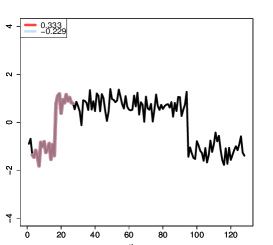
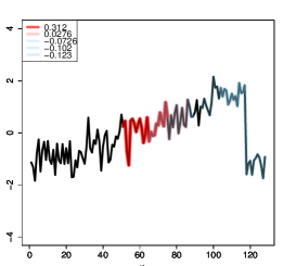
(cylinder) (bell)

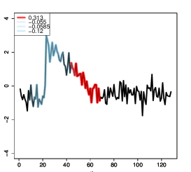
(funnel)

Figure 1: Examples of the visualization of maximizers for a CBF time-series data. Black lines are original time series. We highlight each subsequence that maximizes the similarity with some shapelet in a classifier. Subsequences with positive values (red) contribute to the positive class and subsequences with negative values (blue) contribute to the negative class.

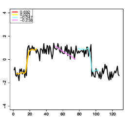
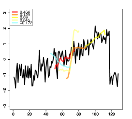
(cylinder) (bell)

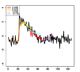
(funnel)

Figure 2: Examples of the visualization of shapelets for a CBF time-series data. The colored lines show important patterns of the obtained classifier. Positive values on the colored lines (red to yellow) indicate the contribution rate for the positive class, and negative values (blue to purple) indicate the contribution rate for the negative class.

7.2 Results for Multiple-Instance Data

We selected the baselines of MIL algorithms as mi-SVM and MI-SVM [2], and MILES [7]. mi-SVM and MI-SVM are classical method in MIL, but still perform favorably compared with state-of-the-art methods for standard multiple-instance data [see, e.g., 12]. The details of the datasets are shown in Table 4.

mi- and MI-SVM find a single but an optimized shapelet ${\bf u}$ which is not limited to the instance in the training sample. The classifiers obtained by these algorithms are formulated as:

$$g(B)=\max_{x\in B}\langle{\bf u},\Phi(x)\rangle=\max_{x\in B}\sum_{z\in P_{S}}\alpha_{z}K(z,x).$$ (12)

MILES finds the multiple-shapelets, but they are limited to the instances in the training sample. The classifier of MILES is formulated as follows:

$$g(B)=\sum_{z\in P_{S}}w_{z}\max_{x\in B}K(z,x).$$ (13)

We used the implementation provided by Doran for mi-SVM and MI-SVM. We combined the Gaussian kernel with mi-SVM and MI-SVM. Parameter $C$ was chosen from $\{1,10,\linebreak[0]100,1000,10000\}$. For our method and MILES, we chose $\nu$ from $\{0.5,\allowbreak 0.3,0.2,0.15,0.1\}$, and we only used the Gaussian kernel. Furthermore, we chose $\sigma$ from $\{0.005,\allowbreak 0.01,0.05,0.1,0.5,1.0\}$. We use $100$-means clustering with respect to each class to reduce $P_{S}$. To avoid the randomness of $k$-means, we ran 30 times of training and selected the model which achieved the best training accuracy. For efficiency, we demonstrated the weak learning problem OP 2. For all these algorithms, we estimated optimal parameter set via 5-fold cross-validation. We used well-known multiple-instance data as shown on the left-hand side of Table 5. The accuracies resulted from 10 times of 5-fold cross-validation.

Table 4: Details of MIL datasets.

dataset	sample size	# instances	dimension
MUSK1	$92$	$476$	$166$
MUSK2	$102$	$6598$	$166$
elephant	$200$	$1391$	$230$
fox	$200$	$1320$	$230$
tiger	$200$	$1220$	$230$

Table 5: Classification accuracies for MIL datasets.

dataset	mi-SVM	MI-SVM	MILES	Ours
MUSK1	$0.834\pm 0.084$	$0.820\pm 0.081$	$\bf 0.865\pm 0.068$	$0.844\pm 0.076$
MUSK2	$0.749\pm 0.082$	$0.840\pm 0.074$	$0.871\pm 0.072$	$\bf 0.879\pm 0.067$
elephant	$0.785\pm 0.070$	$0.823\pm 0.056$	$0.796\pm 0.068$	$\bf 0.828\pm 0.061$
fox	$0.618\pm 0.069$	$0.578\pm 0.075$	${\bf 0.675\pm 0.071}$	$0.646\pm 0.063$
tiger	$0.752\pm 0.078$	$0.815\pm 0.055$	${\bf 0.827\pm 0.057}$	$0.817\pm 0.058$

Table 6: Training accuracies for MIL datasets.

dataset	MILES	Ours
MUSK1	$0.987$	$0.985$
MUSK2	$0.980$	$0.993$
elephant	$0.963$	$0.993$
fox	$0.987$	$0.995$
tiger	$0.973$	$0.993$

Table 7: Training time (sec.) for MIL datasets.

dataset	mi-SVM	MI-SVM	MILES	Ours
MUSK1	$29.6$	$28.1$	$0.584$	$5.57$
MUSK2	$3760.1$	$3530.0$	$103.1$	$80.5$
elephant	$240.6$	$130.3$	$5.84$	$8.30$
fox	$201.9$	$139.2$	$5.4$	$26.4$
tiger	$158.5$	$118.0$	$4.6$	$9.8$

Table 8: Testing time (sec.) for MIL datasets.

dataset	mi-SVM	MI-SVM	MILES	Ours
MUSK1	$0.010$	$0.004$	$0.011$	$0.045$
MUSK2	$0.577$	$0.063$	$0.129$	$0.083$
elephant	$0.053$	$0.015$	$0.067$	$0.115$
fox	$0.078$	$0.025$	$0.118$	$0.145$
tiger	$0.059$	$0.012$	$0.065$	$0.118$

The results are shown in Table 5. MILES and Ours achieve significantly better performance than mi- and MI-SVM. Ours achieves comparable performance to MILES. Table 6 shows the training accuracies of MILES and Ours. It can be seen that Ours achieves higher training accuracy. This result is theoretically reasonable because our hypothesis class is richer than MILES. However, in other words, this means that Ours has a higher overfitting risk than MILES.

Table 7 shows that the training time of the five methods. It is clear that MILES and Ours are more efficient than mi- and MI-SVM. The main reason is that mi- and MI-SVM solve Quadratic Programming (QP) problem while MILES and Ours solve LP problems. MILES worked averagely more efficient than Ours. However, for MUSK2 which has a large number of instances, Ours worked more efficiently than MILES.

The testing time of each algorithm is shown in Table 8. We can see that Ours is comparable to the other algorithms.

8 Conclusion and Future Work

We proposed a new MIL formulation that provides a richer class of the final classifiers based on infinitely many shapelets. We derived the tractable formulation over infinitely many shapelets with theoretical support, and provided an algorithm based on LPBoost and DC (Difference of Convex) algorithm. Our result gives theoretical justification for some existing shapelet-based classifiers [e.g., 7, 17]. The experimental results demonstrate that the provided approach uniformly works for SL and MIL tasks without introducing domain-specific parameters and heuristics, and compares with the baselines of shapelet-based classifiers.

Especially for time-series classification, the number of instances usually becomes large. Although we took a heuristic approach in the experiment, we think it is not an essential solution to improve the efficiency. We preliminarily implemented OP 1 with Orthogonal Random Features [37] that can approximate the Gaussian kernel accurately. It allows us to solve the primal problem of OP 1 directly, and allows us to avoid constructing a large kernel matrix. The implementation improved the efficiency drastically; however, it did not achieve high accuracy as compared with solutions of OP 2 with the heuristics. For SL tasks, there are many successful efficient methods using some heuristics specialized in time-series domain [20, 25, 16, 34, 18, 19]. We will explore many ways to improve efficiency for SL tasks.

Moreover, we would like to improve the generalization error bound. Our bound is still incomparable with the existing bound. Since we think it requires to study more complex analysis, we reserve this for future work. Our heuristics might reduce the model complexity (i.e., the risk of overfitting); however, we do not know how the complexity can be reduced by our heuristics theoretically. To apply our method to various domains, we would like to explore the general techniques for reducing overfitting risk of our method.

A Proof of Theorem 1

First, we give a definition for convenience.

Definition 1

[The set $\Theta$ of mappings from a bag to an instance]
Given a sample $S=(B_{1},\dots,B_{m})$. For any ${\bf u}\in U$, let $\theta_{{\bf u},\Phi}:\{B_{1},\ldots,B_{m}\}\to{\mathcal{X}}$ be a mapping defined by

$$\theta_{{\bf u},\Phi}(B_{i}):=\arg\max_{x\in B_{i}}\left\langle{\bf u},\Phi\left(x\right)\right\rangle,$$

and we define the set of all $\theta_{{\bf u},\Phi}$ for $S$ as $\Theta_{S,\Phi}=\{\theta_{{\bf u},\Phi}\mid{\bf u}\in U\}$. For the sake of brevity, $\theta_{{\bf u},\Phi}$ and $\Theta_{S,\Phi}$ will be abbreviated as $\theta_{{\bf u}}$ and $\Theta$, respectively.

Below we give a proof of Theorem 1.

Proof  We can rewrite the optimization problem (7) by using $\theta\in\Theta$ as follows:

$$\max_{\theta\in\Theta}\max_{{\bf u}\in{\mathbb{H}}:\theta_{\bf u}=\theta}\quad \sum_{i=1}^{m}y_{i}d_{i}\left\langle{\bf u},\Phi\left(\theta(B_{i})\right)\right\rangle$$ (14)

sub.to $$\|{\bf u}\|_{\mathbb{H}}^{2}\leq 1.$$

Thus, if we fix $\theta\in\Theta$, we have a sub-problem. Since the constraint $\theta=\theta_{\bf u}$ can be written as the number $|P_{S}|$ of linear constraints (i.e., sub.to $\langle{\bf u},\Phi(x)\rangle\leq\langle{\bf u},\Phi(\theta(B_{i}))\rangle\;(i\in[m],x\in B_{i})$), each sub-problem is equivalent to a convex optimization. Indeed, each sub-problem can be written as the equivalent unconstrained minimization (by neglecting constants in the objective)

$$\min_{{\bf u}\in{\mathbb{H}}}~{} \beta\|{\bf u}\|^{2}_{\mathbb{H}}-\sum_{i=1}^{m}\sum_{x\in B_{i}}\eta_{i,x}\left(\left\langle{\bf u},\Phi\left(\theta(B_{i})\right)\right\rangle-\left\langle{\bf u},\Phi(x)\right\rangle\right)-\sum_{i=1}^{m}y_{i}d_{i}\left\langle{\bf u},\Phi\left(\theta(B_{i})\right)\right\rangle$$

where $\beta$ and $\eta_{i,x}$ $(i\in[m],x\in B_{i})$ are the corresponding positive constants. Now for each sub-problem, we can apply the standard Representer Theorem argument [see, e.g., 23]). Let ${\mathbb{H}}_{1}$ be the subspace $\{{\bf u}\in{\mathbb{H}}\mid{\bf u}=\sum_{z\in P_{S}}\alpha_{z}\Phi(z),\alpha_{z}\in\mathbb{R}\}$. We denote ${\bf u}_{1}$ as the orthogonal projection of ${\bf u}$ onto ${\mathbb{H}}_{1}$ and any ${\bf u}\in{\mathbb{H}}$ has the decomposition ${\bf u}={\bf u}_{1}+{\bf u}^{\perp}$. Since ${\bf u}^{\perp}$ is orthogonal w.r.t. ${\mathbb{H}}_{1}$, $\|{\bf u}\|_{\mathbb{H}}^{2}=\|{\bf u}_{1}\|_{\mathbb{H}}^{2}+\|{\bf u}^{\perp}\|_{\mathbb{H}}^{2}\geq\|{\bf u}_{1}\|_{\mathbb{H}}^{2}$. On the other hand, $\left\langle{\bf u},\Phi\left(z\right)\right\rangle=\left\langle{\bf u}_{1},\Phi\left(z\right)\right\rangle$. Therefore, the optimal solution of each sub-problem has to be contained in ${\mathbb{H}}_{1}$. This implies that the optimal solution, which is the maximum over all solutions of sub-problems, is contained in ${\mathbb{H}}_{1}$ as well.  

B Proof of Theorem 2

We use $\theta$ and $\Theta$ of Definition 1.

Definition 2

[The Rademacher and the Gaussian complexity [5]]
Given a sample $S=(x_{1},\dots,x_{m})\in{\mathcal{X}}^{m}$, the empirical Rademacher complexity ${\mathfrak{R}}(H)$ of a class $H\subset\{h:{\mathcal{X}}\to\mathbb{R}\}$ w.r.t. $S$ is defined as ${\mathfrak{R}}_{S}(H)=\frac{1}{m}\mathop{\rm E}\limits_{{\boldsymbol{\sigma}}}\left[\sup_{h\in H}\sum_{i=1}^{m}\sigma_{i}h(x_{i})\right]$, where ${\boldsymbol{\sigma}}\in\{-1,1\}^{m}$ and each $\sigma_{i}$ is an independent uniform random variable in $\{-1,1\}$. The empirical Gaussian complexity ${\mathfrak{G}}_{S}(H)$ of $H$ w.r.t. $S$ is defined similarly but each $\sigma_{i}$ is drawn independently from the standard normal distribution.

The following bounds are well-known.

Lemma 1

[Lemma 4 of [5]] ${\mathfrak{R}}_{S}(H)=O({\mathfrak{G}}_{S}(H))$.

Lemma 2

[Corollary 6.1 of [23]] For fixed $\rho$, $\delta>0$, the following bound holds with probability at least $1-\delta$: for all $f\in{\mathrm{conv}(H)}$,

$${\mathcal{E}}_{D}(f)\leq{\mathcal{E}}_{\rho}(f)+\frac{2}{\rho}{\mathfrak{R}}_{S}(H)+3\sqrt{\frac{\log\frac{1}{\delta}}{2m}}.$$

To derive generalization bound based on the Rademacher or the Gaussian complexity is quite standard in the statistical learning theory literature and applicable to our classes of interest as well. However, a standard analysis provides us sub-optimal bounds.

Lemma 3

Suppose that for any $z\in{\mathcal{X}}$, $\|\Phi(z)\|_{\mathbb{H}}\leq R$. Then, the empirical Gaussian complexity of $H_{U}$ with respect to $S$ for $U\subseteq\{{\bf u}\mid\|{\bf u}\|_{\mathbb{H}}\leq 1\}$ is bounded as follows:

$${\mathfrak{G}}_{S}(H)\leq\frac{R\sqrt{(\sqrt{2}-1)+2(\ln|\Theta|)}}{\sqrt{m}}.$$

Proof  Since $U$ can be partitioned into $\bigcup_{\theta\in\Theta}\{{\bf u}\in U\mid\theta_{\bf u}=\theta\}$,

$${\mathfrak{G}}_{S}(H_{U}) =\frac{1}{m}\mathop{\rm E}\limits_{{\boldsymbol{\sigma}}}\left[\sup_{\theta\in\Theta}\sup_{{\bf u}\in U:\theta_{{\bf u}}=\theta}\sum_{i=1}^{m}\sigma_{i}\left\langle{\bf u},\Phi\left(\theta(B_{i})\right)\right\rangle\right]$$

$$=\frac{1}{m}\mathop{\rm E}\limits_{{\boldsymbol{\sigma}}}\left[\sup_{\theta\in\Theta}\sup_{{\bf u}\in U:\theta_{{\bf u}}=\theta}\left\langle{\bf u},\left(\sum_{i=1}^{m}\sigma_{i}\Phi\left(\theta(B_{i})\right)\right)\right\rangle\right]$$

$$\leq\frac{1}{m}\mathop{\rm E}\limits_{{\boldsymbol{\sigma}}}\left[\sup_{\theta\in\Theta}\sup_{{\bf u}\in U}\left\langle{\bf u},\left(\sum_{i=1}^{m}\sigma_{i}\Phi\left(\theta(B_{i})\right)\right)\right\rangle\right]$$

$$\leq\frac{1}{m}\mathop{\rm E}\limits_{{\boldsymbol{\sigma}}}\left[\sup_{\theta\in\Theta}\left\|\sum_{i=1}^{m}\sigma_{i}\Phi\left(\theta(B_{i})\right)\right\|_{\mathbb{H}}\right]$$

$$=\frac{1}{m}\mathop{\rm E}\limits_{{\boldsymbol{\sigma}}}\left[\sup_{\theta\in\Theta}\sqrt{\left\|\sum_{i=1}^{m}\sigma_{i}\Phi\left(\theta(B_{i})\right)\right\|_{\mathbb{H}}^{2}}\right]$$

$$=\frac{1}{m}\mathop{\rm E}\limits_{{\boldsymbol{\sigma}}}\left[\sqrt{\sup_{\theta\in\Theta}\left\|\sum_{i=1}^{m}\sigma_{i}\Phi\left(\theta(B_{i})\right)\right\|_{\mathbb{H}}^{2}}\right]$$

$$\leq\frac{1}{m}\sqrt{\mathop{\rm E}\limits_{{\boldsymbol{\sigma}}}\left[\sup_{\theta\in\Theta}\left\|\sum_{i=1}^{m}\sigma_{i}\Phi\left(\theta(B_{i})\right)\right\|_{\mathbb{H}}^{2}\right]}.$$ (15)

The first inequality is derived from the relaxation of ${\bf u}$, the second inequality is due to Cauchy-Schwarz inequality and the fact $\|{\bf u}\|_{{\mathbb{H}}}\leq 1$, and the last inequality is due to Jensen’s inequality. We denote by ${\boldsymbol{\mathrm{K}}}^{(\theta)}$ the kernel matrix such that ${\boldsymbol{\mathrm{K}}}_{ij}^{(\theta)}=\langle\Phi((\theta(B_{i})),\Phi(\theta(B_{j}))\rangle$. Then, we have

$$\mathop{\rm E}\limits_{{\boldsymbol{\sigma}}}\left[\sup_{\theta\in\Theta}\left\|\sum_{i=1}^{m}\sigma_{i}\Phi\left(\theta(B_{i})\right)\right\|_{\mathbb{H}}^{2}\right]=\mathop{\rm E}\limits_{{\boldsymbol{\sigma}}}\left[\sup_{\theta\in\Theta}\sum_{i,j=1}^{m}\sigma_{i}\sigma_{j}{\boldsymbol{\mathrm{K}}}_{ij}^{(\theta)}\right].$$ (16)

We now derive an upper bound of the r.h.s. as follows.

For any $c>0$,

$$\exp\left(c\mathop{\rm E}\limits_{{\boldsymbol{\sigma}}}\left[\sup_{\theta\in\Theta}\sum_{i,j=1}^{m}\sigma_{i}\sigma_{j}{\boldsymbol{\mathrm{K}}}_{ij}^{(\theta)}\right]\right)$$

$$\leq\mathop{\rm E}\limits_{{\boldsymbol{\sigma}}}\left[\exp\left(c\sup_{\theta\in\Theta}\sum_{i,j=1}^{m}\sigma_{i}\sigma_{j}{\boldsymbol{\mathrm{K}}}_{ij}^{(\theta)}\right)\right]$$

$$= \mathop{\rm E}\limits_{{\boldsymbol{\sigma}}}\left[\sup_{\theta\in\Theta}\exp\left(c\sum_{i,j=1}^{m}\sigma_{i}\sigma_{j}{\boldsymbol{\mathrm{K}}}_{ij}^{(\theta)}\right)\right]$$

$$\leq\sum_{\theta\in\Theta}\mathop{\rm E}\limits_{{\boldsymbol{\sigma}}}\left[\exp\left(c\sum_{i,j=1}^{m}\sigma_{i}\sigma_{j}{\boldsymbol{\mathrm{K}}}_{ij}^{(\theta)}\right)\right]$$

The first inequality is due to Jensen’s inequality, and the second inequality is due to the fact that the supremum is bounded by the sum. By using the symmetry property of ${\boldsymbol{\mathrm{K}}}^{(\theta)}$, we have $\sum_{i,j=1}^{m}\sigma_{i}\sigma_{j}{\boldsymbol{\mathrm{K}}}_{ij}^{(\theta)}={\boldsymbol{\sigma}}^{\top}{\boldsymbol{\mathrm{K}}}^{(\theta)}{\boldsymbol{\sigma}}$, which is rewritten as

$$\top{{\boldsymbol{\sigma}}}{\boldsymbol{\mathrm{K}}}^{(\theta)}{\boldsymbol{\sigma}}=\top{(\top{{\boldsymbol{\mathrm{V}}}}{\boldsymbol{\sigma}})}\left(\begin{array}[]{ccc}\lambda_{1}^{(\theta)}&\hfill\hfil&0\\ \hfill\hfil&\ddots&\hfill\hfil\\ 0&\hfill\hfil&\lambda_{m}^{(\theta)}\\ \end{array}\right)\top{{\boldsymbol{\mathrm{V}}}}{\boldsymbol{\sigma}},$$

where $\lambda_{1}^{(\theta)}\geq\dots\geq\lambda_{m}^{(\theta)}\geq 0$ are the eigenvalues of ${\boldsymbol{\mathrm{K}}}^{(\theta)}$ and ${\boldsymbol{\mathrm{V}}}=({{\bf v}}_{1},\ldots,{{\bf v}}_{m})$ is the orthonormal matrix such that ${{\bf v}}_{i}$ is the eigenvector that corresponds to the eigenvalue $\lambda_{i}$. By the reproductive property of Gaussian distribution, $\top{{\boldsymbol{\mathrm{V}}}}{\boldsymbol{\sigma}}$ obeys the same Gaussian distribution as well. So,

$$\sum_{\theta\in\Theta}\mathop{\rm E}\limits_{{\boldsymbol{\sigma}}}\left[\exp\left(c\sum_{i,j=1}^{m}\sigma_{i}\sigma_{j}{\boldsymbol{\mathrm{K}}}_{ij}^{(\theta)}\right)\right]$$

$$= \sum_{\theta\in\Theta}\mathop{\rm E}\limits_{{\boldsymbol{\sigma}}}\left[\exp\left(c\top{{\boldsymbol{\sigma}}}{\boldsymbol{\mathrm{K}}}^{(\theta)}{\boldsymbol{\sigma}}\right)\right]$$

$$= \sum_{\theta\in\Theta}\mathop{\rm E}\limits_{{\boldsymbol{\sigma}}}\left[\exp\left(c\sum_{k=1}^{m}\lambda_{k}^{(\theta)}(\top{{{\bf v}}_{k}}{\boldsymbol{\sigma}})^{2}\right)\right]$$

$$= \sum_{\theta\in\Theta}\Pi_{k=1}^{m}\mathop{\rm E}\limits_{\sigma_{k}}\left[\exp\left(c\lambda_{k}^{(\theta)}\sigma_{k}^{2}\right)\right]~{}~{}(\text{replace}~{}{\boldsymbol{\sigma}}=\top{{{\bf v}}_{k}}{\boldsymbol{\sigma}})$$

$$= \sum_{\theta\in\Theta}\Pi_{k=1}^{m}\left(\int_{-\infty}^{\infty}\exp\left(c\lambda_{k}^{(\theta)}\sigma^{2}\right)\frac{\exp(-\sigma^{2})}{\sqrt{2\pi}}d\sigma\right)$$

$$= \sum_{\theta\in\Theta}\Pi_{k=1}^{m}\left(\int_{-\infty}^{\infty}\frac{\exp(-(1-c\lambda_{k}^{(\theta)})\sigma^{2})}{\sqrt{2\pi}}d\sigma\right).$$

Now we replace $\sigma$ by $\sigma^{\prime}=\sqrt{1-c\lambda_{k}^{(\theta)}}\sigma$. Since $d\sigma^{\prime}=\sqrt{1-c\lambda_{k}^{(\theta)}}d\sigma$, we have:

$$\int_{-\infty}^{\infty}\frac{\exp(-(1-c\lambda_{k}^{(\theta)})\sigma^{2})}{\sqrt{2}\pi}d\sigma=\frac{1}{\sqrt{2\pi}}\int_{-\infty}^{\infty}\frac{\exp(-\sigma^{\prime 2})}{\sqrt{1-c\lambda_{k}^{(\theta)}}}d\sigma^{\prime}$$

$$= \frac{1}{\sqrt{1-c\lambda_{k}^{(\theta)}}}.$$

Now, applying the inequality that $\frac{1}{\sqrt{1-x}}\leq 1+2(\sqrt{2}-1)x$ for $0\leq x\leq\frac{1}{2}$, the bound becomes

$$\exp\left(c\mathop{\rm E}\limits_{{\boldsymbol{\sigma}}}\left[\sup_{\theta\in\Theta}\sum_{i,j=1}^{m}\sigma_{i}\sigma_{j}{\boldsymbol{\mathrm{K}}}_{ij}^{(\theta)}\right]\right)$$

$$\leq \sum_{\theta\in\Theta}\Pi_{k=1}^{m}\left(1+2(\sqrt{2}-1)c\lambda_{k}^{(\theta)}+2\lambda_{1}\right).$$ (17)

Further, taking logarithm, dividing the both sides by $c$, letting $c=\frac{1}{2\max_{k}\lambda_{k}^{(\theta)}}=1/(2\lambda_{1}^{(\theta)})$, fix $\theta=\theta^{*}$ such that $\theta^{*}$ maximizes (B), and applying $\ln(1+x)\leq x$, we get:

$$\mathop{\rm E}\limits_{{\boldsymbol{\sigma}}}\left[\sup_{\theta\in\Theta}\sum_{i,j=1}^{m}\sigma_{i}\sigma_{j}{\boldsymbol{\mathrm{K}}}_{ij}^{(\theta^{*})}\right]$$

$$\leq(\sqrt{2}-1)\sum_{k=1}^{m}\lambda_{k}^{(\theta^{*})}+2\lambda_{1}^{(\theta^{*})}\ln|\Theta|$$

$$=(\sqrt{2}-1)\top{({\boldsymbol{\mathrm{K}}}^{(\theta^{*})})}+2\lambda_{1}^{(\theta^{*})}\ln|\Theta|$$

$$\leq(\sqrt{2}-1)mR^{2}+2mR^{2}\ln|\Theta|,$$ (18)

where the last inequality holds since $\lambda_{1}^{(\theta^{*})}=\|{\boldsymbol{\mathrm{K}}}^{(\theta^{*})}\|_{2}\leq m\|{\boldsymbol{\mathrm{K}}}^{(\theta)}\|_{\max}\leq R^{2}$. By Equation (B) and (B), we have:

$${\mathfrak{G}}_{S}(H) \leq\frac{1}{m}\sqrt{\mathop{\rm E}\limits_{{\boldsymbol{\sigma}}}\left[\sup_{\theta\in\Theta}\sum_{i,j=1}^{m}\sigma_{i}\sigma_{j}{\boldsymbol{\mathrm{K}}}_{ij}^{(\theta)}\right]}$$

$$\leq\frac{R\sqrt{(\sqrt{2}-1)+2\ln|\Theta|}}{\sqrt{m}}.$$

 

Thus, it suffices to bound the size $|\Theta|$. The basic idea to get our bound is the following geometric analysis. Fix any $i\in[m]$ and consider points $\{\Phi(x)\mid x\in B_{i}\}$. Then, we define equivalence classes of ${\bf u}$ such that $\theta_{\bf u}(i)$ is in the same class, which define a Voronoi diagram for the points $\{\Phi(x)\mid x\in B_{i}\}$. Note here that the similarity is measured by the inner product, not a distance. More precisely, let $\{V_{i}(x)\mid x\in B_{i}\}$ be the Voronoi diagram, each of the region is defined as $V_{i}(x)=\{{\bf u}\in{\mathbb{H}}\mid\theta_{{\bf u}}(B_{i})=x\}$ Let us consider the set of intersections $\bigcap_{i\in[m]}V_{i}{(x_{i})}$ for all combinations of $(x_{1},\ldots,x_{m})\in B_{1}\times\cdots\times B_{m}$. The key observation is that each non-empty intersection corresponds to a mapping $\theta_{{\bf u}}\in\Theta$. Thus, we obtain $|\Theta|=(\text{the number of intersections $\bigcap_{i\in[m]}V_{i}(x_{i})$})$. In other words, the size of $\Theta$ is exactly the number of rooms defined by the intersections of $m$ Voronoi diagrams $V_{1},\dots,V_{m}$. From now on, we will derive upper bound based on this observation.

Lemma 4

$$|\Theta|=O(|P_{S}|^{2d_{\Phi,S}^{*}}).$$

Proof  We will reduce the problem of counting intersections of the Voronoi diagrams to that of counting possible labelings by hyperplanes for some set. Note that for each neighboring Voronoi regions, the border is a part of hyperplane since the closeness is defined in terms of the inner product. Therefore, by simply extending each border to a hyperplane, we obtain intersections of halfspaces defined by the extended hyperplanes. Note that, the size of these intersections gives an upper bound of intersections of the Voronoi diagrams. More precisely, we draw hyperplanes for each pair of points in $\Phi(P_{S})$ so that each point on the hyperplane has the same inner product between two points. Note that for each pair $\Phi(z),\Phi(z^{\prime})\in P_{S}$, the normal vector of the hyperplane is given as $\Phi(z)-\Phi(z^{\prime})$ (by fixing the sign arbitrary). Thus, the set of hyperplanes obtained by this procedure is exactly ${\Phi_{\mathrm{diff}}(P_{S})}$. The size of ${\Phi_{\mathrm{diff}}(P_{S})}$ is ${|P_{S}|}\choose 2$, which is at most $|P_{S}|^{2}$. Now, we consider a “dual” space by viewing each hyperplane as a point and each point in $U$ as a hyperplane. Note that points ${\bf u}$ (hyperplanes in the dual) in an intersection give the same labeling on the points in the dual domain. Therefore, the number of intersections in the original domain is the same as the number of the possible labelings on ${\Phi_{\mathrm{diff}}(P_{S})}$ by hyperplanes in $U$. By the classical Sauer’s Lemma and the VC dimension of hyperplanes [see, e.g., Theorem 5.5 in 28]), the size is at most $O((|P_{S}|^{2})^{d_{\Phi,S}^{*}})$.  

Theorem 4

1. For any $\Phi$, $|\Theta|=O(|P_{S}|^{8(R/\mu^{*})^{2}})$.

2. if ${\mathcal{X}}\subseteq\mathbb{R}^{\ell}$ and $\Phi$ is the identity mapping over $P_{S}$, then $|\Theta|=O(|P_{S}|^{\min\{8(R/\mu^{*})^{2},2\ell\}}\})$.

3. if ${\mathcal{X}}\subseteq\mathbb{R}^{\ell}$ and $\Phi$ satisfies that $\left\langle\Phi(z),\Phi(x)\right\rangle$ is monotone decreasing with respect to $\|z-x\|_{2}$ (e.g., the mapping defined by the Gaussian kernel) and $U=\{\Phi(z)\mid z\in{\mathcal{X}}\subseteq\mathbb{R}^{\ell},\|\Phi(z)\|_{\mathbb{H}}\leq 1\}$, then $|\Theta|=O(|P_{S}|^{\min\{8(R/\mu^{*})^{2},2\ell\}}\})$.

Proof  (i) We follow the argument in Lemma 4. For the set of classifiers $F=\{f:{\Phi_{\mathrm{diff}}(P_{S})}\to\{-1,1\}\mid f={\mathrm{sign}}(\langle{\bf u},{{\bf v}}\rangle),\|{\bf u}\|_{\mathbb{H}}\leq 1,\min_{{{\bf v}}\in{\Phi_{\mathrm{diff}}(P_{S})}}|\langle{\bf u},{{\bf v}}\rangle|=\mu\}$, its VC dimension is known to be at most $R^{2}/\mu^{2}$ for ${\Phi_{\mathrm{diff}}(P_{S})}\subseteq\{{{\bf v}}\mid\|{{\bf v}}\|_{\mathbb{H}}\leq 2R\}$ [see, e.g., 28]). By the definition of $\mu^{*}$, for each intersection given by hyperplanes, there always exists a point ${\bf u}$ whose inner product between each hyperplane is at least $\mu^{*}$. Therefore, the size of the intersections is bounded by the number of possible labelings in the dual space by $U^{\prime\prime}=\{{\bf u}\in{\mathbb{H}}\mid\|{\bf u}\|_{\mathbb{H}}\leq 1,\min_{{{\bf v}}\in{\Phi_{\mathrm{diff}}(P_{S})}}|\langle{\bf u},{{\bf v}}\rangle|=\mu^{*}\}$. Thus, we obtain that $d_{\Phi,S}^{*}$ is at most $8(R/\mu^{*})^{2}$ and by Lemma 4, we complete the proof of case (i).

(ii) In this case, the Hilbert space ${\mathbb{H}}$ is contained in $\mathbb{R}^{\ell}$. Then, by the fact that VC dimension $d_{\Phi,S}^{*}$ is at most $\ell$ and Lemma 4, the statement holds.

(iii) If $\left\langle\Phi(z),\Phi(x)\right\rangle$ is monotone decreasing for $\|z-x\|$, then the following holds:

$$\arg\max_{x\in{\mathcal{X}}}\left\langle\Phi(z),\Phi(x)\right\rangle=\arg\min_{x\in{\mathcal{X}}}\|z-x\|_{2}.$$

Therefore, $\max_{{\bf u}:\|{\bf u}\|_{\mathbb{H}}=1}\langle{\bf u},\Phi(x)\rangle=\|\Phi(x)\|_{\mathbb{H}}$, where ${\bf u}=\frac{\Phi(x)}{\|\Phi(x)\|_{\mathbb{H}}}$. It indicates that the number of Voronoi cells made by $V(x)=\{z\in\mathbb{R}^{\ell}\mid z=\arg\max_{x\in B}(z\cdot x)\}$ corresponds to the $\hat{V}(x)=\{\Phi(z)\in{\mathbb{H}}\mid z=\arg\max_{x\in B}\langle\Phi(z),\Phi(x)\rangle\}$. Then, by following the same argument for the linear kernel case, we get the same statement.  
Now we are ready to prove Theorem 2.

Proof [Proof of Theorem 2] By using Lemma 1, and 2, we obtain the generalization bound in terms of the Gaussian complexity of $H$. Then, by applying Lemma 3 and Theorem 4, we complete the proof.  

B.1 Hyper-parameter tuning for time-series classification

. In the experiment for time series classification, we roughly tuned $\nu$ and $\sigma^{2}$ of the Gaussian kernel. As we mentioned before, we need high computation time when learning very large time series. The main computational cost is to iteratively solve weak learning problems by using an LP (or QP) solver. The number of constraints of the optimization problem (9) depends on the total number of instances in negative bags. Therefore, in the hyper-parameter tuning phase, we finish solving each weak learning problem by obtaining the solution of the optimization problem (11). Using the rough weak learning problem, we tuned $\nu$ and $\sigma$ through a grid search via three runs of $3$-fold cross validation.

References

- Andrews and Hofmann [2004] Andrews, S. and Hofmann, T. (2004). Multiple instance learning via disjunctive programming boosting. In Advances in Neural Information Processing Systems, pages 65–72.
- Andrews et al. [2003] Andrews, S., Tsochantaridis, I., and Hofmann, T. (2003). Support vector machines for multiple-instance learning. In Advances in Neural Information Processing Systems, pages 577–584.
- Auer and Ortner [2004] Auer, P. and Ortner, R. (2004). A boosting approach to multiple instance learning. In European Conference on Machine Learning, pages 63–74.
- Bagnall et al. [2017] Bagnall, A., Lines, J., Bostrom, A., Large, J., and Keogh, E. (2017). The great time series classification bake off: a review and experimental evaluation of recent algorithmic advances. Data Mining and Knowledge Discovery, 31(3):606–660.
- Bartlett and Mendelson [2003] Bartlett, P. L. and Mendelson, S. (2003). Rademacher and gaussian complexities: Risk bounds and structural results. Journal of Machine Learning Research, 3:463–482.
- Carbonneau et al. [2018] Carbonneau, M.-A., Cheplygina, V., Granger, E., and Gagnon, G. (2018). Multiple instance learning: A survey of problem characteristics and applications. Pattern Recognition, 77:329 – 353.
- Chen et al. [2006] Chen, Y., Bi, J., and Wang, J. Z. (2006). Miles: Multiple-instance learning via embedded instance selection. IEEE Transactions on Pattern Analysis and Machine Intelligence, 28(12):1931–1947.
- Chen et al. [2015] Chen, Y., Keogh, E., Hu, B., Begum, N., Bagnall, A., Mueen, A., and Batista, G. (2015). The ucr time series classification archive. www.cs.ucr.edu/~eamonn/time_series_data/.
- Cuturi [2011] Cuturi, M. (2011). Fast global alignment kernels. In International conference on machine learning, pages 929–936.
- Demiriz et al. [2002] Demiriz, A., Bennett, K. P., and Shawe-Taylor, J. (2002). Linear Programming Boosting via Column Generation. Machine Learning, 46(1-3):225–254.
- Dietterich et al. [1997] Dietterich, T. G., Lathrop, R. H., and Lozano-Pérez, T. (1997). Solving the multiple instance problem with axis-parallel rectangles. Artificial Intelligence, 89(1-2):31–71.
- Doran [2015] Doran, G. (2015). Multiple Instance Learning from Distributions. PhD thesis, Case WesternReserve University.
- Doran and Ray [2014] Doran, G. and Ray, S. (2014). A theoretical and empirical analysis of support vector machine methods for multiple-instance classification. Machine Learning, 97(1-2):79–102.
- Gärtner et al. [2002] Gärtner, T., Flach, P. A., Kowalczyk, A., and Smola, A. J. (2002). Multi-instance kernels. In International Conference on Machine Learning, pages 179–186.
- Grabocka et al. [2014] Grabocka, J., Schilling, N., Wistuba, M., and Schmidt-Thieme, L. (2014). Learning time-series shapelets. In ACM SIGKDD International Conference on Knowledge Discovery and Data Mining, pages 392–401.
- Grabocka et al. [2015] Grabocka, J., Wistuba, M., and Schmidt-Thieme, L. (2015). Scalable discovery of time-series shapelets. CoRR, abs/1503.03238.
- Hills et al. [2014] Hills, J., Lines, J., Baranauskas, E., Mapp, J., and Bagnall, A. (2014). Classification of time series by shapelet transformation. Data Mining and Knowledge Discovery, 28(4):851–881.
- Hou et al. [2016] Hou, L., Kwok, J. T., and Zurada, J. M. (2016). Efficient learning of timeseries shapelets. In AAAI Conference on Artificial Intelligence,, pages 1209–1215.
- Karlsson et al. [2016] Karlsson, I., Papapetrou, P., and Boström, H. (2016). Generalized random shapelet forests. Data Mining and Knowledge Discovery, 30(5):1053–1085.
- Keogh and Rakthanmanon [2013] Keogh, E. J. and Rakthanmanon, T. (2013). Fast shapelets: A scalable algorithm for discovering time series shapelets. In International Conference on Data Mining, pages 668–676.
- Le Thi and Pham Dinh [2018] Le Thi, H. A. and Pham Dinh, T. (2018). DC programming and DCA: thirty years of developments. Mathematical Programming, 169(1):5–68.
- Löning et al. [2019] Löning, M., Bagnall, A., Ganesh, S., Kazakov, V., Lines, J., and Király, F. J. (2019). sktime: A unified interface for machine learning with time series.
- Mohri et al. [2012] Mohri, M., Rostamizadeh, A., and Talwalkar, A. (2012). Foundations of Machine Learning. The MIT Press.
- Platt et al. [2000] Platt, J. C., Cristianini, N., and Shawe-Taylor, J. (2000). Large margin DAGs for multiclass classification. In Advances in Neural Information Processing Systems, pages 547–553.
- Renard et al. [2015] Renard, X., Rifqi, M., Erray, W., and Detyniecki, M. (2015). Random-shapelet: an algorithm for fast shapelet discovery. In IEEE International Conference on Data Science and Advanced Analytics, pages 1–10.
- Sabato and Tishby [2012] Sabato, S. and Tishby, N. (2012). Multi-instance learning with any hypothesis class. Journal of Machine Learning Research, 13(1):2999–3039.
- Sangnier et al. [2016] Sangnier, M., Gauthier, J., and Rakotomamonjy, A. (2016). Early and reliable event detection using proximity space representation. In International Conference on Machine Learning, pages 2310–2319.
- Schölkopf and Smola [2002] Schölkopf, B. and Smola, A. (2002). Learning with Kernels: Support Vector Machines, Regularization, Optimization, and Beyond. Adaptive Computation and Machine Learning. MIT Press.
- Shapiro [2009] Shapiro, A. (2009). Semi-infinite programming, duality, discretization and optimality conditions. Optimization, 58(2):133–161.
- Shimodaira et al. [2001] Shimodaira, H., Noma, K.-i., Nakai, M., and Sagayama, S. (2001). Dynamic time-alignment kernel in support vector machine. In International Conference on Neural Information Processing Systems, pages 921–928.
- Tao and Souad [1988] Tao, P. D. and Souad, E. B. (1988). Duality in D.C. (Difference of Convex functions) Optimization. Subgradient Methods, pages 277–293.
- Tavenard et al. [2017] Tavenard, R., Faouzi, J., and Vandewiele, G. (2017). tslearn: A machine learning toolkit dedicated to time-series data. https://github.com/rtavenar/tslearn.
- Warmuth et al. [2008] Warmuth, M., Glocer, K., and Rätsch, G. (2008). Boosting algorithms for maximizing the soft margin. In Advances in Neural Information Processing Systems, pages 1585–1592.
- Wistuba et al. [2015] Wistuba, M., Grabocka, J., and Schmidt-Thieme, L. (2015). Ultra-fast shapelets for time series classification. CoRR, abs/1503.05018.
- Ye and Keogh [2009] Ye, L. and Keogh, E. (2009). Time series shapelets: A new primitive for data mining. In ACM SIGKDD International Conference on Knowledge Discovery and Data Mining, pages 947–956.
- Yu and Joachims [2009] Yu, C.-N. J. and Joachims, T. (2009). Learning structural svms with latent variables. In International Conference on Machine Learning, pages 1169–1176.
- Yu et al. [2016] Yu, F. X. X., Suresh, A. T., Choromanski, K. M., Holtmann-Rice, D. N., and Kumar, S. (2016). Orthogonal random features. In Advances in Neural Information Processing Systems, pages 1975–1983.
- Zhang et al. [2006] Zhang, C., Platt, J. C., and Viola, P. A. (2006). Multiple instance boosting for object detection. In Advances in Neural Information Processing Systems, pages 1417–1424.
- Zhang et al. [2013] Zhang, D., He, J., Si, L., and Lawrence, R. (2013). MILEAGE: Multiple instance learning with global embedding. In International Conference on Machine Learning, pages 82–90.